strong motion simulation using stochastic green’s...

Strong Motion Simulation using Stochastic Green’s Function Method

Index 1. Outline of Simulation of Strong Ground Motion Using Stochastic Green’s Function

Methods 2. Examples of the way how to select the velocity model 3. Examples of Simulation.

3.1 Example 1: The 2007 Noto Hanto Earthquake, Japan (Mw 6.7) 3.2 Example 2: The 2005 Kashmir Earthquake, Pakistan (Mw 7.6) 3.3 Example 3: The 2003 Boumerdes Earthquake, Algeria (Mw 6.9) 3.4 Example 4: The 1997 Zirkuh Earthquake, Iran (Mw 7.2) 3.5 Example 5: The 2003 Tokachi-oki Earthquake, Japan (Mw 8.2)

4. Calculated Results

1. Outline of Simulation of Strong Ground Motion Using Stochastic Green’s Function Methods

1.1 Introduction Strong ground motion simulation is conducted using Stochastic Green’s Function Method (SGFM) with several assumptions mentioned below. Therefore, the calculated waveforms and parameters of ground motion are tentative ones. It is expected that these will be improved by replacing the assumed parameters with the corresponding observed ones obtained by local studies.

The keys of SGFM are appropriate underground structural models of the crust, deep ground and shallow ground and also the asperity models calibrated by strong motion data obtained near to earthquake sources. For both of them, high activities of local researchers are required both in the field of seismology and earthquake engineering.

1.2 Green’s Function The term: “Green’s function” in the elasto-dynamic wave theory means the displacement at a point due to a point force acting at another point and is a tensor that has 3 by 3 components. Observed waves do not have to be displacement always, but can be velocity and/or acceleration. In such cases, the terms “velocity Green’s function” and/or “acceleration Green’s function” are used respectively. The input does not have to be a point body force, but can be traction. The term elasto-dynamic Green’s function have to be used with the description of the input and the observed waves. 1.2.1 Empirical Green’s Function In Seismology, however, records of small earthquakes that share the source area and observation station with the main shock are often called Empirical Green’s Function (EGF). EGF shares the path and the local amplification effects with the main shock but has significant difference in the source effect (Hartzell, 1978). This difference has been called the relation of small and big

earthquakes. ω-2 model of the source spectra (Aki, 1967) and the scaling law of the fault parameters (Kanamori & Anderson, 1975) gives the way to estimate this relation for earthquakes up to intermediate size: Mw about 6 (e. g., Yokoi & Irikura, 1991; Architectual Institute of Japan, 1992).

For larger earthquakes, heterogeneous rupture has to be considered (e. g., Kikuchi & Fukao, 1987). The parts of earthquake source fault that emit the seismic waves stronger than the rest is called Asperities (e. g., Boatwright, 1988). Applying ω-2 model of the source spectra to asperities, strong ground motion due to big earthquakes can be synthesized. This way is called

Empirical Green’s Function Method (EGFM). EGFM can be applied without any information about local amplification effect that affects much the waveforms, because this is already included in EGF (e. g., Irikura, 1986; Irikura & Kamae, 1994).

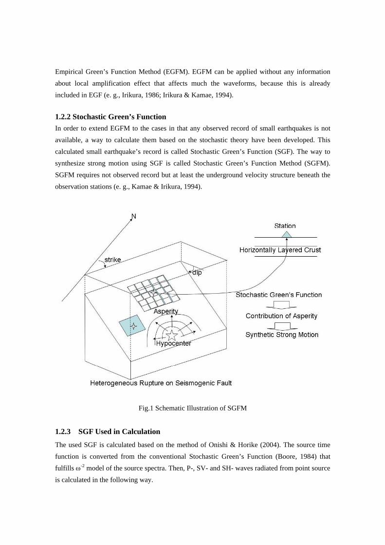
1.2.2 Stochastic Green’s Function In order to extend EGFM to the cases in that any observed record of small earthquakes is not available, a way to calculate them based on the stochastic theory have been developed. This calculated small earthquake’s record is called Stochastic Green’s Function (SGF). The way to synthesize strong motion using SGF is called Stochastic Green’s Function Method (SGFM). SGFM requires not observed record but at least the underground velocity structure beneath the observation stations (e. g., Kamae & Irikura, 1994).

Fig.1 Schematic Illustration of SGFM

1.2.3 SGF Used in Calculation

The used SGF is calculated based on the method of Onishi & Horike (2004). The source time function is converted from the conventional Stochastic Green’s Function (Boore, 1984) that fulfills ω-2 model of the source spectra. Then, P-, SV- and SH- waves radiated from point source is calculated in the following way.

The path effect is given by the geometrical spreading effect, scattering effect and the radiation pattern of body waves. The former is estimated by the ray tracing method (Cerveny et al., 1997). Therefore, only body waves are taken into account. For the latter, the effect of scattering during propagation is taken into account. For the propagation distance much shorter than the wave length, the theoretical radiation coefficients are used, whereas for that much longer than the wave length, their convergent values estimated by the scattering theory are used. For intermediate case, the linear interpolation between these two cases is used. The used thresholds for the ratio of the propagation distance to the wavelength are 0.5 and 5.0 as well as Onishi & Horike (2004).

The local amplification effect is calculated using the given horizontally layered media beneath observation stations and the incident angles calculated by the ray theory for P-, SV- and SH-waves as mentioned above (Silva, 1976).

The velocity models used vary case by case. For few of them, PS-logging data are available but for others only crustal velocity structure model such as CRUST2.

The above mentioned SGF is used in place of EGF in EGFM. The slip velocity function proposed by Irikura et al. (1997) is used. SGF is calculated for each asperity by locating its point source at the center of asperity. The effect of background region is not calculated because it usually does not affect significantly to acceleration waveforms.

1.3 Synthesis of waveform for the main shock

1.3.1 Asperity Model used in Calculation The asperity models used also vary case by case. For few cases, the asperity model determined by strong motion synthesis using EGFM is already given. For others the asperity models are obtained from the result of the source inversion: e. g., the slip distribution along the rectangular fault plane such as those given by the earthquake catalog in IISEE web site and Finite Source Rupture Model Data Base (SRCMOD). The asperities are extracted to enclose fault elements of which slip is 1.5 or more times larger than the average one over the fault and is subdivided if any row or column has an average less than 1.5 times the average one. Then, this asperity is trimmed until all of the edges have an average slip equal to or larger than 1.25 times the slip averaged over the entire rupture area (Somerville et al., 1999).

Besides the location, width, length, strike, dip and rake of the fault, a fixed value is used for the upper limit of the seismogenic zone (Ito, 1999) because of the lack of information.

1.3.2 Waveform Synthesis The way of waveform synthesis is the same as usual EGFM using observed small earthquake

data. It is different from the original way of Onishi and Horike (2004). Namely, SGF calculated beforehand is used in place of small earthquake of EGFM. NS, EW and UD components of SGF are converted to transverse, radial and vertical ones. Then the radiation pattern coefficient for SH-wave including the scattering effect is used for transverse component to correct the effect of difference of azimuth between SGF and fault elements, whereas for radial and vertical components, the P-SV coefficient of radiation pattern is used for correction. The corrected waveforms are converted back to NS, EW and UD components before the superposition of SGF. In this calculation, P- and S- waves are not separately handled and waveform synthesis is conducted considering only the propagation of S-wave. This means the synthesis of vertical component is out of scope.

1.4 Other considerations The high frequency cut-off of acceleration spectra fmax is fixed at 6 Hz for all cases. Upper limit of the seismogenic zone is set at few Km of which depth varies case by case,

In some cases, the location of seismic faults appeared at ground surface and the corresponding epicenter’s location listed in earthquake catalogs do not coincide each other. The discrepancy is also found between hypocenter’s location and the corresponding results of the source inversion. The former is not always located on the fault plane of the latter. In case that the information about the fault scarp is available, location and orientation of fault plane is corrected according to this information. Location of the rupture starting point of source inversion result is considered independent from hypocenter location in seismic catalogs.

References Aki, K. (1967), Scaling Law of Seismic Spectrum, J. Geophys. Res., 72, 1217-1231. Architectual Institute of Japan, Earthquake Motion and Ground Conditions, 1992 Boatwright, J. (1988), The Seismic Radiation from Computer Models of Faulting, Bull. Seism.

Soc. Am., 78, 489-508. Boore, D. M. (1983), Stochastic Simulation of High-Frequency Ground Motion Based on

Seismological Models of Radiated Spectra, Bull. Seism. Soc. Am., 173, 1865-1894. Cerveny, V., I. A. Molotokov & I. Psencik (1997), Ray Method in Seismology, Univerzita

Karlova Praha. Finite Source Rupture Model Data Base, ETH, Switzerland,

http://www.seismo.ethz.ch/static/srcmod/ Hartzell, S. H. (1978), Earthquake Aftershocks as Green’s Functions, Geophis. Res. Lett., 5,

1-4.

IISEE’s CMTs, Aftershock Distributions, Fault planes, and Rupture processes for recent large earthquakes in the world, IISEE, BRI, Japan, http://iisee.kenken.go.jp/eqcat/Top_page_en.htm

Irikura, K. (1986), Prediction of Strong Acceleration Motion using Empirical Green’s Function,

Proc. 7th Japan Earthquake Engineering Symposium、151-156.

Irikura, K. & K. Kamae, (1994), Estimation of Strong Ground Motion in Broad-Frequency Band Based on a Seismic Source Scaling Model and an Empirical Green’s Function Technique, ANNALI DI GEOFISICA, XXXVII, 25-47.

Irikura, K., T. Kagawa & H. Sekiguchi (1997), Revision of the Empirical Green’s Function Method by Irikura (1986), Programme and Abstracts of The Seismological Society of Japan 1997 No.2, Seismological Society of Japan, B25

Ito, K (1999), Seismogenic Layer, Reflective Lower Crust, Surface Heat Flow and Large Inland- Earthquakes, Tectonophysics, 306, 423-433.

Kanamori, H. & D. L. Anderson, (1972), Theoretical Basis of Some Empirical Relations in Seismology, Bull. Seism. Soc. Am., 65, 1073-1095.

Kamae, K. & K. Irikura, (1994), Simulation of Seismic Intensity Distribution During the 1946 Nankai Earthquake Using a Stochastically Simulated Green’s Function, Proc. of 9th Japan Earthquake Engineering Symposium, 1, 559-564.

Kikuchi, M. & Y. Fukao (1987), Inversion of Long-Period P-waves from Great Earthquakes along Subduction Zones, Tectonophysics, 144, 231-247.

Onishi, Y. & M. Horike (2004), The Extended Stochastic Simulation Method for Close-Fault Earthquake Motion Prediction and Comments for its Application to the Hybrid Method.

Silva, W. (1976), Body Waves in a Layered Anelastic Solid, Bull. Seism. Soc. Am., 66, 1539-1554.

Somerville, P., K. Irikura, R. Graves, S. Sawada, D. Wald, N. Abrahamson, Y. Iwasaki, T. Kagawa, N. Smith & A. Kowada (1999), Characterizing earthquake heterogeneous slip models for the prediction of strong motion, Seism. Res. Lett., 70, 59-80.

Yokoi, T. & K. Irikura (1991), Empirical Green’s Function Technique Based on the Scaling Law of Source Spectra, Zisin, Ser. 2, 44, 109-122(In Japanese with English Abstract).

2. Examples of the way how to select the velocity model.

2.1 Local Underground Velocity Structure Models

The most recommendable way is to use:

the shallow underground structural model of soft soils (Vs<400-700m/s) for each points

where the ground motion is calculated,

the structural model of sedimentary layers obtained by geophysical methods in the study

area, and

the crustal model obtained by the crustal study in or close to the study area,

If the shallow one is not available it is not possible to estimate the ground motion at the ground

surface correctly. The output from the calculation must be the ground motion at the top of the

engineering bedrock (Vs<400-700m/s). If consideration on the non-linear behavior of soils is

required, it is also recommendable to calculate the ground motion at the top of the engineering

bedrock and then use it for the input to the software for non-linear simulation of layered soils, e.

g., DYNEQ.

For the second and the third ones, the P-wave and S-wave velocity structures being used in

seismic observation network for hypocenter determination can be good references.

If they are not available an alternative way may be to use the global model, i. e., structures

averaged over an area as wide as 1X1 or 2X2 degrees. Two examples are shown below. It must

be noted that the calculated results have the limitations due to the usage of inaccurate structures.

Especially, in study areas close to the plate boundaries and the border region between land and

ocean, i. e., continental shelves underground structures can suffer a considerable distortion and

then the calculated ground motion also.

2.2 Empirical formulas of the relation between density and P- and S-wave velocities.

The following two relations are used for unconsolidated sediments.

Ludwig et al.(1970): Density = 1.2475 + 0.399 Vp - 0.026 Vp2.

Kitsubezaki et al.(1990) for sedimentary layers saturated by underground water:

Vp = 1.11 Vs +1200 (m/s)

Assumption Vp/Vs=1.732 can describe the general characteristics of the materials that compose

the earth crust and the mantle. This corresponds to= where and are Lame’s constants.

Kitsunezaki, C., N. Goto, Y. Kobayashi, T. Ikawa, M. Horike, T. Saito, T. Kuroda, K.

Yamane, and K. Okuzumi, 1990, Estimation of P- and S-wave velocities in deep soil

deposits for evaluating ground vibrations in earthquake, Journal of Japan Society for Natural

Disaster Science, 9, 1–17 (in Japanese with English abstract).

Ludwig, W. J., J. E. Nafe and C. L. Drake, 1970, Seismic refraction, A. E. Maxwell (ed.),

The Sea, Vol. 4, Wiley-Interscience, New York, 53-84.

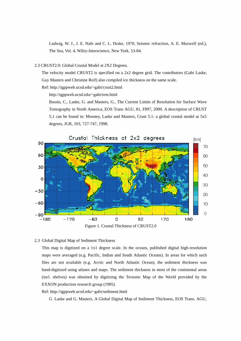
2.3 CRUST2.0: Global Crustal Model at 2X2 Degrees.

The velocity model CRUST2 is specified on a 2x2 degree grid. The contributors (Gabi Laske,

Guy Masters and Christine Reif) also compiled ice thickness on the same scale.

Ref: http://igppweb.ucsd.edu/~gabi/crust2.html

http://igppweb.ucsd.edu/~gabi/rem.html

Bassin, C., Laske, G. and Masters, G., The Current Limits of Resolution for Surface Wave

Tomography in North America, EOS Trans AGU, 81, F897, 2000. A description of CRUST

5.1 can be found in: Mooney, Laske and Masters, Crust 5.1: a global crustal model at 5x5

degrees, JGR, 103, 727-747, 1998.

Figure 1. Crustal Thickness of CRUST2.0

2.3 Global Digital Map of Sediment Thickness

This map is digitized on a 1x1 degree scale. In the oceans, published digital high-resolution

maps were averaged (e.g. Pacific, Indian and South Atlantic Oceans). In areas for which such

files are not available (e.g. Arctic and North Atlantic Ocean), the sediment thickness was

hand-digitized using atlases and maps. The sediment thickness in most of the continental areas

(incl. shelves) was obtained by digitizing the Tectonic Map of the World provided by the

EXXON production research group (1985).

Ref: http://igppweb.ucsd.edu/~gabi/sediment.html

G. Laske and G. Masters, A Global Digital Map of Sediment Thickness, EOS Trans. AGU,

http://igppweb.ucsd.edu/~gabi/crust2.html

http://igppweb.ucsd.edu/~gabi/sediment.html

78, F483, 1997.

Ludwig, W.F., J.E. Nafe and C.L. Drake, Seismic Refraction, in "The Sea, Vol. 4, Ideas and

Observations on Progress in the Study of the Seas", A.E. Maxwell (ed.), Wiley-Interscience,

New York, 1970.

Mooney, W.D., G. Laske and G. Masters, CRUST5.1: A global crustal model at 5°x5°. J.

Geophys. Res., 103, 727-747, 1998.

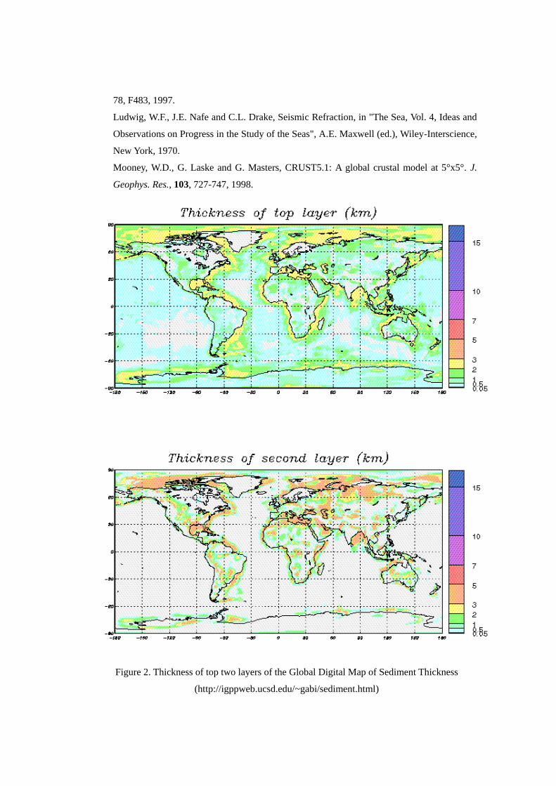
Figure 2. Thickness of top two layers of the Global Digital Map of Sediment Thickness

(http://igppweb.ucsd.edu/~gabi/sediment.html)

3. Examples of Simulation using SGFM Five examples are shown. For all of them, non-linear effect is not taken into account. They are not examples of real strong motion evaluation but just examples to show the difference of calculated waveform depending on the available information. The underground structures are divided into three parts: the crustal structure, the deep ground structure below the engineering bedrock and above upper limit of the crust, and the shallow ground structure above engineering bedrock. The shear wave velocity below the boundary between the first and the second is typically Vs~3000 m/sec and that between the second and third is Vs~400-700 m/sec. The grade of the information of underground structures differs site by site.

The fifth example, however, shows the limitation of the calculation method of SGF.

3.1 Example 1: The 2007 Noto Hanto Earthquake, Japan (Mw 6.7)

It is expected that the underground structural models used in calculation are close to the reality, except non-linearity of shallow layers. Crustal structure is referred from that used by the seismic observatory in the same region. Deep ground structure is referred from J-SHIS that is the velocity structure database for whole Japan based on the compilation of the geophysical and seismic observation as much as possible. The shallow ground structure is referred from the PS-logging data exactly at each site. The asperity model of the seismic source used is determined by the EGFM using aftershock waveform. Namely it is calibrated within the frequency range of the engineering interest and the SGFM calculation. Therefore, this example shows what the SGFM can do.

3.2 Example 2: The 2005 Kashmir Earthquake, Pakistan (Mw 7.6) The underground structural model couldn’t be found for any of three parts. Therefore, the global crustal model CRUST2 is referred and other two structures are not used. Namely, the calculated results are given at the top of the crust. The asperity is extracted from the source model that is referred from the result of inversion using tele-seismic waveform data but only the frequency component much lower than the engineering interest and the SGFM calculation. The location of the source fault is corrected using the result of interpretation of satellite image.

3.3 Example 3: The 2003 Boumerdes Earthquake, Algeria (Mw 6.9) The underground structure used by the local seismic observatory is used for calculation. This covers two deeper parts of structure but the shallow ground structure couldn’t be found. The asperity is extracted from the source model that is referred from the result of inversion using GPS observation, leveling data and strong motion data but only the frequency component lower than the engineering interest and SGFM

calculation. 3.4 Example 4: The 1997 Zirkuh Earthquake, Iran (Mw 7.2)

The underground structural model couldn’t be found for any of three parts. Therefore, the global crustal model CRUST2 is referred and other two structures are not used. Namely, the calculated results are given at the top of the crust. The asperity is extracted from the source model that is referred from the result of inversion using tele-seismic waveform data but only the frequency component much lower than the engineering interest and SGFM calculation. The location of the source fault is corrected using the result of in-site geological and/or geomorphologic survey of the fault scarp.

3.5 Example 5: The 2003 Tokachi-oki Earthquake, Japan (Mw 8.2) Crustal structure is referred from that used for source inversion. Deep ground structure is referred from J-SHIS that is the velocity structure database for whole Japan based on the compilation of the geophysical and seismic observation as much as possible. The shallow ground structure is referred from the PS-logging data exactly at each site. The asperity model of the seismic source used is determined by the EGFM using aftershock waveform. Different from other examples, the stations are located far from the focal points of SGF. Therefore, the setting of the quality factors of the crust plays a significant role.

These examples clearly show the importance of the studies of local and regional underground structures including velocities, density and the quality factors. Also the strong motion observations at near-field are necessary to obtain the asperity model and/or the strong motion generation area. All these are necessary to obtain an acceptable calculation result within the frequency range of the engineering interest.

It is recommendable to promote the strong motion observation not only at soil sites but also at rock site and the studies of underground structure of above mentioned three parts using various geophysical methods by the researchers of each country and each region.

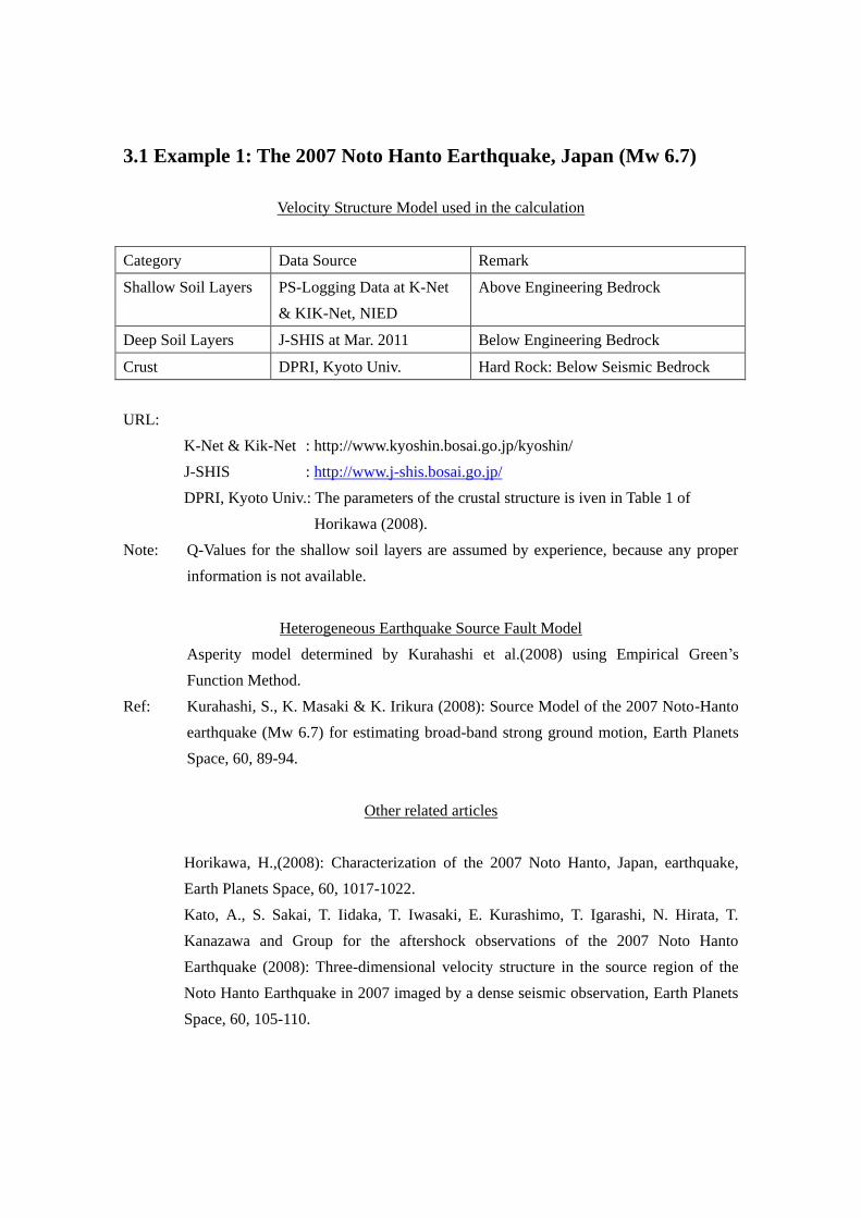
3.1 Example 1: The 2007 Noto Hanto Earthquake, Japan (Mw 6.7)

Velocity Structure Model used in the calculation

Category Data Source Remark

Shallow Soil Layers PS-Logging Data at K-Net

& KIK-Net, NIED

Above Engineering Bedrock

Deep Soil Layers J-SHIS at Mar. 2011 Below Engineering Bedrock

Crust DPRI, Kyoto Univ. Hard Rock: Below Seismic Bedrock

URL:

K-Net & Kik-Net : http://www.kyoshin.bosai.go.jp/kyoshin/

J-SHIS : http://www.j-shis.bosai.go.jp/

DPRI, Kyoto Univ.: The parameters of the crustal structure is iven in Table 1 of

Horikawa (2008).

Note: Q-Values for the shallow soil layers are assumed by experience, because any proper

information is not available.

Heterogeneous Earthquake Source Fault Model

Asperity model determined by Kurahashi et al.(2008) using Empirical Green’s

Function Method.

Ref: Kurahashi, S., K. Masaki & K. Irikura (2008): Source Model of the 2007 Noto-Hanto

earthquake (Mw 6.7) for estimating broad-band strong ground motion, Earth Planets

Space, 60, 89-94.

Other related articles

Horikawa, H.,(2008): Characterization of the 2007 Noto Hanto, Japan, earthquake,

Earth Planets Space, 60, 1017-1022.

Kato, A., S. Sakai, T. Iidaka, T. Iwasaki, E. Kurashimo, T. Igarashi, N. Hirata, T.

Kanazawa and Group for the aftershock observations of the 2007 Noto Hanto

Earthquake (2008): Three-dimensional velocity structure in the source region of the

Noto Hanto Earthquake in 2007 imaged by a dense seismic observation, Earth Planets

Space, 60, 105-110.

http://www.j-shis.bosai.go.jp/

3.2 Oct. 8, 2005 Kashmir Earthquake, Pakistan (Mw 7.5)



Shallow Soil Layers Not Available Above Engineering Bedrock

Deep Soil Layers Not Available Below Engineering Bedrock

Crust Category RB of CRUST2 Hard Rock: Below Seismic Bedrock

URL:

CRUST2: http://igppweb.ucsd.edu/~gabi/crust2.html

Note: .


URL: IISEE Earthquake Catalog

http://iisee.kenken.go.jp/cgi-bin/eqcatalog/frame_eng.cgi?j_no=101&chk1=on&c

hk1_1=on&chk1_2=on&chk1_3=on&chk2=on&chk2_0=on&chk2_1=on&chk3=

on&p_no=1

Note: Asperities are extracted using the algorithm given by Somerville et al. (1999)

from the slip distribution given by Prof. Yagi, Tsukuba Univ..

Ref: Somerville, P., K. Irikura, R. Graves, S. Sawada, D. Wald, N. Abrahamson,

Y. Iwasaki, T. Kagawa, N. Smith & A. Kowada (1999), Characterizing

earthquake heterogeneous slip models for the prediction of strong motion,

Seism. Res. Lett., 70, 59-80..


Avouac, J.-P., F. Ayoub, S. Leprince, O. Konca, D. V. Helmberger (2006). The

2005, Mw 7.6 Kashmir earthquake: Sub-pixel correlation of ASTER images and

seismic waveforms analysis, Earth and Planetary Science Letters, 249,

514–528.

3.3 2003 Boumerdes Earthquake, Algeria (Mw 6.9)



Shallow Soil Layers No/A Above Engineering Bedrock

Deep Soil Layers CRAAG Below Engineering Bedrock

Crust Hard Rock: Below Seismic Bedrock

URL:

CRAAG: http://www.craag.dz/

The structure model is given in Semmane et al.(2005)

Note: The top layer of the velocity model has Vp=4.5 Km/s and Vs=2.09 Km/s and

must be categorized as hard rock.

The velocity model used is included in the downloaded file from Finite Source

Rupture Model Database


URL: Finite Source Rupture Model Database

http://www.seismo.ethz.ch/static/srcmod/

Ref: Semmane, F.,M. Campillo, and F. Cotton (2005): Fault location and source

process of the Boumerdes, Algeria, earthquake inferred from geodetic and

strong motion data, GEOPHYS. RES. LETT., 32, L01305,

doi:10.1029/2004GL021268.


from the slip distribution downloaded from Finite Source Rupture Model

Database.






Laouami, N., A. Slimani, Y. Bouhadad, J.-L. Chatelain, A. Nour (2006).

http://www.craag.dz/

Evidence for fault-related directionality and localized site effects from strong

motion recordings of the 2003 Boumerdes (Algeria) earthquake: Consequences

on damage distribution and the Algerian seismic code, Soil Dynamics and

Earthquake Engineering, 26, 991–1003

3.4 Oct. 8, 2005 Kashmir Earthquake, Pakistan (Mw 7.5)



Shallow Soil Layers Not Available Above Engineering Bedrock

Deep Soil Layers Not Available Below Engineering Bedrock

Crust Category P6 of CRUST2 Hard Rock: Below Seismic Bedrock

URL:

CRUST2: http://igppweb.ucsd.edu/~gabi/crust2.html

Note: .


URL: IISEE Earthquake Catalog

http://iisee.kenken.go.jp/cgi-bin/eqcatalog/frame_eng.cgi


from the slip distribution given by Prof. Yagi, Tsukuba Univ..






Berberian, M., J. A. Jackson, M. Qorashi, M. M. Khatib, K. Priestley, M.

Talebian and M. Ghafuri-Ashtiani (1999).The 1997May 10 Zirkuh (Qa'enat)

earthquake (Mw 7.2) : faulting along the Sistan suture zone of eastern Iran,

Geophys. J. Int., 136, 671-694.

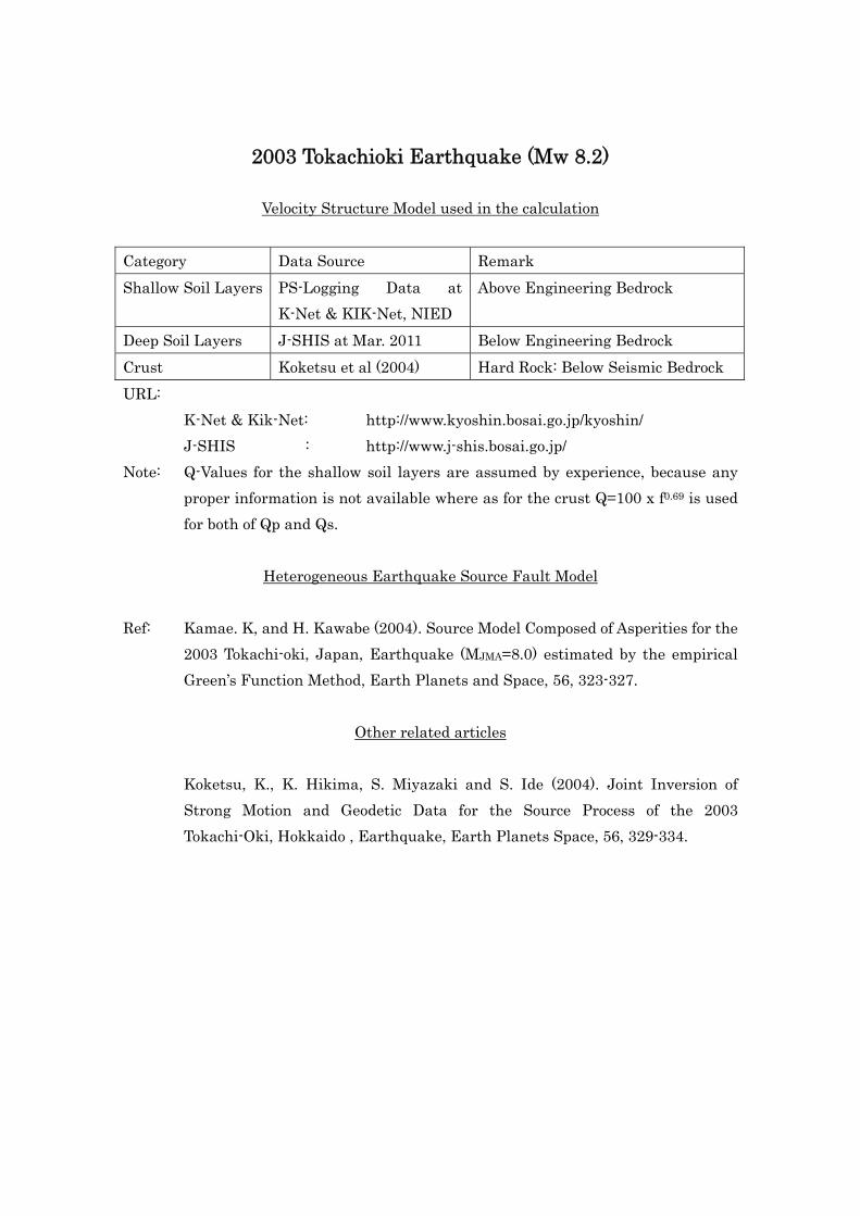
2003 Tokachioki Earthquake (Mw 8.2)

Velocity Structure Model used in the calculation Category Data Source Remark Shallow Soil Layers PS-Logging Data at

K-Net & KIK-Net, NIED Above Engineering Bedrock

Deep Soil Layers J-SHIS at Mar. 2011 Below Engineering Bedrock Crust Koketsu et al (2004) Hard Rock: Below Seismic Bedrock URL:

K-Net & Kik-Net: http://www.kyoshin.bosai.go.jp/kyoshin/ J-SHIS : http://www.j-shis.bosai.go.jp/

Note: Q-Values for the shallow soil layers are assumed by experience, because any proper information is not available where as for the crust Q=100 x f0.69 is used for both of Qp and Qs.


Ref: Kamae. K, and H. Kawabe (2004). Source Model Composed of Asperities for the

2003 Tokachi-oki, Japan, Earthquake (MJMA=8.0) estimated by the empirical Green’s Function Method, Earth Planets and Space, 56, 323-327.


Koketsu, K., K. Hikima, S. Miyazaki and S. Ide (2004). Joint Inversion of Strong Motion and Geodetic Data for the Source Process of the 2003 Tokachi-Oki, Hokkaido , Earthquake, Earth Planets Space, 56, 329-334.

strong motion simulation using stochastic green’s...

Documents