approximate separability of green’s function …zhao/homepage/publication_files/rank.pdf ·...
TRANSCRIPT
APPROXIMATE SEPARABILITY OF GREEN’S FUNCTION FOR HIGH
FREQUENCY HELMHOLTZ EQUATIONS
BJORN ENGQUIST AND HONGKAI ZHAO
Abstract. Approximate separable representations of Green’s functions for differentialoperators is a basic and an important aspect in the analysis of differential equations and inthe development of efficient numerical algorithms for solving them. Being able to approx-imate a Green’s function as a sum with few separable terms is equivalent to the existenceof low rank approximation of corresponding discretized system. This property can beexplored for matrix compression and efficient numerical algorithms. Green’s functions forcoercive elliptic differential operators in divergence form have been shown to be highlyseparable and low rank approximation for their discretized systems has been utilized todevelop efficient numerical algorithms. The case of Helmholtz equation in the high fre-quency limit is more challenging both mathematically and numerically. In this work, wedevelop a new approach to study approximate separability for the Green’s function ofHelmholtz equation in the high frequency limit based on an explicit characterization ofthe relation between two Green’s functions and a tight dimension estimate for the bestlinear subspace approximating a set of almost orthogonal vectors. We derive both lowerbounds and upper bounds and show their sharpness for cases that are commonly used inpractice.
1. Introduction
Given a linear differential operator, denoted by L, the Green’s function, denoted byG(x,y), is defined as the fundamental solution in a domain Ω ⊆ Rn to the partial differ-ential equation
(1)
LxG(x,y) = δ(x− y), x,y ∈ Ω ⊆ Rn
with boundary condition or condition at infinity,
where δ(x− y) is the Dirac delta function denoting an impulse source point at y. In par-ticular, general solutions of a partial differential equation can be obtained by superpositionof fundamental solutions with source locations in Ω (and/or boundary of Ω).
Approximate separability of G(x,y) is defined as the following: given two sets X,Y ⊆Ω ⊆ Rd (see Figure 1) and ε > 0, there is a smallest N ε such that there are fl(x), gl(y), l =
The work of Bjorn Engquist is partially supported by NSF grant DMS-1217203 and Texas Consortiumfor Computational Seismology.
The work of Hongkai Zhao is partially supported by NSF grant DMS-1115698 and ONR grant N00014-11-1-0602.
1

2 BJORN ENGQUIST AND HONGKAI ZHAO
1, 2, . . . , N ε
(2)
∥∥∥∥∥G(x,y)−Nε∑l=1
fl(x)gl(y)
∥∥∥∥∥X×Y
≤ ε, x ∈ X,y ∈ Y,
where ‖ · ‖X×Y is the norm of some function space which G, fl, gl belong to. If X and Yare compact and disjoint domains in Rd and G(x,y) is continuous in X×Y , which is oftenthe case of practical interest, there exists a polynomial approximation of G(x,y) in X ×Yby Weierstrass approximation theorem which is separable. So there is a N ε < ∞ for anyε > 0. The most interesting issue is how N ε depends on ε, which manifests the intrinsiccomplexity of the PDE and its solution within ε-approximation. If one views G(x,y) asa family of functions on X parametrized by y ∈ Y , this is equivalent to saying that theKolmogorov n-width [17] for the family of functions G(x,y) in the ‖ · ‖X normed functionspace is ε when n = N ε. Kolmogorov n-width, which is used to characterize informationcontent in information theory, is the best approximation of a set S in a normed space Wby a n dimensional linear subspace Ln defined as
(3) dn(S,W ) := infLn
supf∈S
infg∈Ln
‖f − g‖W ,
Of course the role of x and y can be reversed.
Ω
X Y
G(x,y)
Figure 1. Green’s function G(x,y) with dependence on x ∈ X and y ∈ Y .
We introduce the following relations to simplify notations in later derivations. x & ymeans that there is a constant ∞ > c > 0 such that x ≥ cy, x . y means that thereis a constant ∞ > C > 0 such that x ≤ Cy, and x ∼ y means there are two constants0 < c ≤ C < ∞ such that cy ≤ x ≤ Cy. For our results for Helmholtz equation (5), allconstants are independent of the wave number k as k →∞.
In this study, we assume X,Y ⊆ Ω are two compact manifolds embedded in Rd with di-mensions dim(X) and dim(Y ) respectively, i.e., they may be compact domains inRd, dim(X) =dim(Y ) = d = 1, 2, 3, or compact two dimensional surfaces embedded in R3 or one dimen-sional compact curves embedded in Rd, d = 2, 3. Without loss of generality, we assumedim(X) ≥ dim(Y ) = s.
One can get a sharper upper bound for N ε based simply on regularity of the Green’sfunction. For example, suppose X,Y are two disjoint compact domains in Rd and G(x,y)
is Cm(X × Y ), one can show that N ε . ε−dm using the following argument. Lay down a

APPROXIMATE SEPARABILITY OF GREEN’S FUNCTION FOR HIGH FREQUENCY HELMHOLTZ EQUATIONS3
uniform grid yj , j = 1, 2, . . . J ∼ ε−dm in Y with a grid size h ∼ ε
1m . ∀y ∈ Y , G(x,y) can
be approximated by (m − 1)-th order interpolation/extrapolation of G(x,yj), which is alinear combination of G(x,yj) and satisfies
(4) |G(·,y)−∑
j:yj∈Bδ(y)
ajG(·,yj)| ≤ ‖Dmy G(·, ·)‖L∞(X×Y )h
m ≤ ε,
where Bδ(y) is a ball centered at y with a radius δ ∼ h. If Y is a rectangular domainand G(x,y), one can even use We call G(x,y) highly separable if N ε depends on ε weekly,N ε ≤ O(| log ε|p), for some p > 0.
When a linear PDE, such as (1), is discretized and numerically solved, high separabil-ity of its Green’s function implies existence of low rank approximation of subsets of thediscretized system, which provides a matrix compression and lies at the heart for manyefficient algorithms. Typically low rank approximation has been used in two ways. Oneway is to utilize low rank approximation of the discretized Green’s function, which is thekernel for boundary integral formulation, for fast matrix vector multiplication when solv-ing boundary integral equations by iterative methods [8, 11, 12, 26, 27]. Similarly, it hasbeen used to develop fast algorithms for evaluation of fast oscillatory scattering operatorand Fourier integral operators [6, 24, 25]. The other way is to utilize low rank propertyto develop fast algorithms to solve a large linear system Ax = b corresponding to a dis-cretization of a PDE such as (1). Each column of the inverse matrix A−1 is a numericalapproximation of the Green’s function. Again low rank approximation for off-diagonalsubmatrices of A−1, which is implied by high separability of the Green’s function on twodisjoint sets, is extensively explored in many fast algorithms to solve the linear system suchas hierarchical matrix and structured inverse methods [2, 3, 7, 15, 23, 29, 31, 32]. Oftenthe low rank approximation is computed or learned on the fly. Fast random algorithmsor rank revealing type of methods [14, 22] can be used to find the leading singular valuesand corresponding singular vectors of a matrix. However, the computation cost increasesdramatically if the rank is not sufficiently low. So both upper and lower bound estimatesfor approximate separability is of crucial importance in these applications.
In the literature, mostly upper bound estimates for highly separable cases were shownfor Green’s functions or kernel functions when developing fast numerical algorithms basedon low rank approximation as mentioned above. These estimates are typically based onconstructive approaches for Green’s functions or kernel functions with explicit expressionand using asymptotic expansion. Interesting study on spatial bandwidth and degree offreedom of scattered field have also been done in the engineering literature [4, 5], whichshows that the scattered field is almost band limited and the degree of freedom is close tothe Nyquist number in term of the effective (spatial) bandwidth of the scattered field and tothe extension of the observation domain. A more general non-constructive mathematicalapproach was developed in [2] to show that the Green’s function for a coercive ellipticoperator in divergence form with L∞-coefficients is highly separable (Theorem 2.8) for twodisjoint domains X,Y based on a key gradient estimate by Caccioppoli inequality. Themethod and result can be extended to Green’s function of more general elliptic equations

4 BJORN ENGQUIST AND HONGKAI ZHAO
with non-dominant lower order terms, such as convection-diffusion equations with smallconvection term or the Helmholtz equation (5) with small wave number k. Their methoddoes not work when the lower order term is dominant which is the case for the Helmholtzequation with large k. It becomes a singularly perturbed problem and the gradient ofthe Green’s function is unbounded almost everywhere as k → ∞ due to fast oscillations.These issues are also reflected in numerical computation for these different PDEs. Itis well known that there are many efficient numerical methods to solve the discretizedsystem corresponding to differential operators that are elliptic dominant, such as iterativemethods with various effective preconditioners and direct inverse methods as mentionedabove. This is related to the intrinsic complexity manifested by the high separability ofthe corresponding Green’s functions. On the other hand, it is well known that Helmholtzequation with large wave number is very difficult to solve numerically in practice. Forexample, all those well developed iterative methods for elliptic equations do not workeffectively for this case [10].
Here we give another mathematics perspective by showing lower bounds for the approxi-mate separability of the Green’s function for Helmholtz equation in high frequency limit interms of both ε and k. The lower bounds, which are sharp for many practical setups, showthat the Green’s function is not highly separable as k → ∞ and manifests the intrinsiccomplexity of the solution space. In our study we give
• explicit characterization of the correlation or angle (in L2 normed space) betweentwo Green’s functions of Helmholtz equation (5) in the high frequency limit,
(‖G(·,y1)‖2‖G(·,y2)‖2)−1
∫XG(x,y1)G(x,y2)dx . (k|y1 − y2|)−α, k|y1 − y2| → ∞
for some α > 0 which depends on the dimension ofX, its geometry and the locationsof y1,y2 (see Theorem 2.1) based on generalized stationary phase analysis.• lower bound estimate for the approximate separability for the Green’s function of
Helmholtz equation in the high frequency limit
N εk &
k2α, α < s
2 ,
ks−δ, α ≥ s2 ,
and upper bound estimate
N εk . k
s+δ
as k →∞ for two compact manifolds X and Y with dim(X) ≥ dim(Y ) = s and anyδ > 0, where the constants in & and . are independent of k for a fixed small ε (seeLemma 3.1 and Theorem 3.1 - 3.4). The lower bound is based on a tight dimensionestimate improved from that for a set of nearly orthogonal random vectors by N.Alon [1] and Johnson-Lindenstraus Lemma [19].• explicit estimates and their sharpness for situations that are commonly used in
practice (see Section 4). Our theory is also applied to show precise conditions ifhigh separability (or low rank approximation after numerical discretization) can orcan not be achieved for special set ups.

APPROXIMATE SEPARABILITY OF GREEN’S FUNCTION FOR HIGH FREQUENCY HELMHOLTZ EQUATIONS5
As far as we know, lower bound estimate for approximate separability of Green’s func-tions of this type is the first in the literature. These bounds mathematically characterizeintrinsic complexities for high frequency wave phenomena. We hope these studies and un-derstandings can provide useful insights for developing fast numerical algorithms as well.
2. Helmholtz equation and its Green’s function
Let G(x,y) be the Green’s function to the Helmholtz equation in free space,
(5) ∆xG(x,y) + k2n2(x)G(x,y) = δ(x− y), x,y ∈ Rd,
where k > 0 is the wave number, 0 < c < n(x) < C < ∞ is the index of refractionand δ(x− y) denotes a point source at y. Suitable far field radiation condition has to besatisfied for uniqueness. The high frequency limit means the wave number k →∞, whichposes challenge both mathematically and numerically due to faster and faster oscillationsin the solution.
For completeness, we provide the general formula for the free space Green’s function ofHelmholtz equation (5) for any space dimension,
(6) G0(x,y) = cdkpH
(1)p (k|x− y|)|x− y|p
, p =d− 2
2, cd =
1
2i(2π)p, x,y ∈ Rd,x 6= y.
H(1)p (r) is the first kind Hankel function of order p which has the following asymptotic
behavior: as r → 0
(7) H(1)p (r) =
− iπΓ(p)
(2r
)p, p 6= 0
2iπ log r, p = 0
where Γ(p) is the Gamma function, and as r →∞
(8) H(1)p (r) =
(2
πr
) 12
ei(r−pπ2−π
4) +O(r−
32 ), p ≥ 0.
For d = 3, the Green’s function takes the simplest form
(9) G0(x,y) =1
4π
eik|x−y|
|x− y|, x 6= y.
For d = 2,
(10) G0(x,y) = − i4H
(1)0 (k|x− y|) = − 1
2π
∫ ∞0
eik|x−y| cosh θdθ, x 6= y,
and
(11) limr→0+
H(1)0 (r) =
2i
πlog r, lim
r→∞H
(1)0 (r) =
√2
πrei(r−π/4) +O(r−3/2).

6 BJORN ENGQUIST AND HONGKAI ZHAO
Denote Bdτ (y) and Sdρ(y) to be a ball and a sphere in Rd centered at y with radius τ
and ρ respectively. We have(12)∫
Bnτ (y)|G0(x,y)|2dx = c2
dk2p
∫ τ
0dρ
∫Sdρ
[H(1)p (kρ)]2
ρ2pds = c2
dωdk2p−2
∫ kτ
0r[H(1)
p (r)]2dr,
where ωd = 2πd2
Γ( d2
)is the area of the unit sphere in Rd. From the asymptotic formula (7),
we see that G0 is square integrable at the singular source for d = 2, 3. Also from the
asymptotic formula (8), we have ‖G0(·,y)‖2(Bnτ (y)) ∼ kd−32 as k →∞.
From the above explicit expressions for free space Green’s function, we see that exceptfor the case d = 3, there is a multiplication factor related to k for the magnitude of theGreen’s function. To characterize the angle or correlation between two Green’s functionand study the separability of the Green’s function without the effect of this factor, wedefine the normalized Green’s function as
(13) G(x,y) =G(x,y)
‖G(·,y)‖2, x ∈ X ⊂ Rd, ‖G(·,y)‖22 =
∫X|G(x,y)|2dx,
in our later study with the following understandings:
• ‖G(·,y)‖2 is a smooth function of y since fast oscillation due to rapid change ofphase function is removed.• When d = 3, all results for the normalized Green’s function G(x,y) can be extended
to G(x,y) since there are constants 0 < c < C <∞ that are independent of k suchthat c < |G(x,y)| < C,∀x ∈ X,y ∈ Y , once two compact sets X,Y ⊂ R3 are fixed.• In this paper we prove results for d = 2, 3 for practical interest. Since the Green’s
function is square integrable at the source singularity, we allow overlaps betweentwo compact domains X and Y when dim(X) = dim(Y ) = d = 2, 3. All results forbounded and disjoint X and Y can be extended to d > 3.
Approximate separability of G(x,y) is defined as in (2) except that we now put a sub-script k in N ε
k to specifically indicate the dependence on k. The key issue is the dependenceon k for a given ε > 0 as k →∞. In practice, such as development of fast algorithms uti-lizing low rank approximation for the discretized system, X and Y are often disjoint andcompact. Typical norms used are either L∞(X × Y ) or L2(X × Y ). In our study wefirst show analysis and results in L2 norm, which fits well with using SVD (singular valuedecomposition) for low rank approximation of a matrix, and then extend those results toL∞ norm. Regarding G(x,y) as a family of functions in L2(X) parametrized by y ∈ Y(see Figure 1), the separability condition (2) in L2(X × Y ) is equivalent to the existenceof a linear subspace SX ⊂ L2(X) with dimension N ε
k such that
(14)
√∫Y‖G(x,y)− PSXG(x,y)‖2L2(X)dy ≤ ε,
where PSXG(x,y) is the projection of G(x,y) in SX . This formulation is the same withthe role of x and y exchanged.

APPROXIMATE SEPARABILITY OF GREEN’S FUNCTION FOR HIGH FREQUENCY HELMHOLTZ EQUATIONS7
We start with the study of approximate separability of the Green’s function, G0(x,y),for homogeneous medium, i.e., n2(x) ≡ 1 in (5), in free space. When 2-norm is used asthe metric, one important geometric characterization of relation between two vectors is theangle or correlation between them. Let X ⊂ R3 be a compact domain and y1,y2 /∈ X betwo points with δ = |y1 − y2| 1. It is easy to see that∣∣∣< G0(·,y1), G0(·,y2) > −1
∣∣∣ =
∣∣∣∣∣ 1
‖G0(·,y1)‖2‖G0(·,y2)‖2
∫X
eik(|x−y1|−|x−y2|)
|x− y1||x− y2|dx− 1
∣∣∣∣∣ . kδwhere the constant in . depends on domain X and the distance between X and y1,y2.In another word, two Green’s functions become more and more correlated when the twosource points become closer and closer. This is true in general for Green’s function aslong as G(x,y) is Lipschitz in y. Actually for strictly elliptic operator of the followingdivergence form in Rd, d ≥ 3,
(15) L = −d∑
i,j=1
∂
∂xj(aij(x)
∂
∂xj), λ|ξ|2 ≤
d∑i,j=1
aij(x)ξiξj ≤ µ|ξ|2,
where aij(x) are bounded measurable functions and 0 < λ ≤ µ < ∞ are two constants,there exists a unique Green’s function [20, 13] G(x,y) satisfying
(16) c(d, λ, µ)|x− y|2−d ≤ G(x,y) ≤ C(d, λ, µ)|x− y|2−d,
where 0 < c(d, λ, µ) < C(d, λ, µ) <∞ are two constants. Given a compact domain X ⊂ Rdand two points y1,y2 /∈ X, define
ρ = min[minx∈X|x− y1|,min
x∈X|x− y2|], K =
C(d, λ, µ)
c(d, λ, µ)
[1 +|y1 − y2|
ρ
]d−2
.
Then we have
G(x,y2)
G(x,y1)≤ C(d, λ, µ)
c(d, λ, µ)
[|x− y1||x− y2|
]d−2
≤ C(d, λ, µ)
c(d, λ, µ)
[|x− y2|+ |y1 − y2|
|x− y2|
]d−2
≤ K,
and vice versa. Given two disjoint compact domains X,Y ⊂ Rd, d ≥ 3, with ρ being thedistance between the two domains and r being the diameter of Y , the correlation betweenany two Green’s function with sources at y1,y2 ∈ Y is bounded by
(17) 1 ≥< G(·,y1), G(·,y2) >X≥ K−2, K =C(d, λ, µ)
c(d, λ, µ)
[1 +
r
ρ
]d−2
.
Also Caccioppoli inequality gives a L2 norm bound of the gradient of the Green’s functionaway from the source singularity which is used in [2] to show that the Green’s function forelliptic operator (and Helmholtz equation with small k) is highly separable. However, thepicture is quite different in the more challenging regime of high frequency limit since theGreen’s function becomes more and more oscillatory as k →∞.

8 BJORN ENGQUIST AND HONGKAI ZHAO
2.1. Decorrelation of Two Green’s Function in High Frequency Limit in Homo-geneous Medium. Here we study the angle between two Green’s functions or how fastthey decorrelate in term of the ratio of the separation distance of the two source pointswith respect to the wave length due to fast oscillations. Stationary phase theory will playan important role here. Define
(18) φ(x) = |y1 − y2|−1(|x− y1| − |x− y2|).
We have |φ(x)| ≤ 1 and
(19)
∇φ(x) = |y1 − y2|−1(
x−y1
|x−y1| −x−y2
|x−y2|
)
D2φ(x) = |y1 − y2|−1
[I− (x−y1)|x−y1|
(x−y1)T
|x−y1||x−y1| −
I− (x−y2)|x−y2|
(x−y2)T
|x−y2||x−y2|
].
|∇φ(x)| 6= 0 except for points on the line going through y1,y2 and outside the interval
between y1,y2, where maximum value 1 or minimum value -1 of φ is attained (see Figure
2). Also D2φ(x) is degenerate in the direction of y1 − y2. However, for x on the lineand outside the interval between y1,y2, the Hessian in the plane perpendicular to the line,denoted by D2
⊥, is a multiple of identity matrix I⊥ in the plane,
(20) D2⊥φ(x) =
±1
|x− y1||x− y2|I⊥,
where the sign depends whether maximum or minimum is attained at x.From the stationary phase result [16, 30] for I(k) =
∫eikφ(x)u(x)dx, where u ∈ C∞c (Rd)
and φ(x) has isolated stationary points xm,m = 1, 2, ..M, |∇φ(xm)| = 0 and D2φ(xm)non-degenerate, one has
(21)
|I(k)− (2πk )d/2
∑Mm=1
eikφ(xm)
|det[D2φ(xm)]|1/2 eiπ4
sgn(D2φ(xm))u(xm)|
≤ Ck−d/2−1‖[D2φ(xm)]−1‖d/2+1∑
β≤s+2 ‖Dβu‖L2 ,
where s > d/2 and C is an universal constant independent of φ and u. However, we have tomodify the standard stationary phase technique due to the following three complications inour case: (1) the stationary points may not be isolated, (2) the integration is on a compactdomain X and the integrand u is not C∞0 (X), and (3) there may be singularities in theintegrand. Here is our result.
Theorem 2.1. Assume X ⊂ Rd, d = 2, 3 is a compact domain with piecewise smoothboundary. G0(x,y) is the normalized free space Green’s function. Depending on positionsof y1,y2 relative to X and its boundary, there is some α > 0 such that
(22)∣∣∣< G0(·,y1), G0(·,y2) >
∣∣∣ . (k|y1 − y2|)−α, min1, d− 1
2 ≤ α ≤ d+ 1
2
as k|y1 − y2| → ∞. The constant in . depends on X and the distances from y1,y2 to X.

APPROXIMATE SEPARABILITY OF GREEN’S FUNCTION FOR HIGH FREQUENCY HELMHOLTZ EQUATIONS9
X
y1
y2 r
ξη
y1
y2
X
X
y1
y2
case 1 case 2 case 3
Figure 2. Different positions of y1,y2 relative to X
Proof. We prove for d = 3 first. Define
(23)
k = k|y1 − y2|, φ(x) = |y1 − y2|−1(|x− y1| − |x− y2|),
u(x) = 1‖G0(·,y1)‖2‖G0(·,y2)‖2|x−y1||x−y2| ,
and the operator
(24) L =1
|∇φ(x)|2
3∑j=1
∂φ
∂xj
∂
∂xjLT = −
3∑j=1
∂
∂xj
1
|∇φ(x)|2∂φ
∂xj.
we have
(25)∣∣∣< G0(·,y1), G0(·,y2) >
∣∣∣ =
∣∣∣∣∫Xeikφ(x)u(x)dx
∣∣∣∣Denote the line going through y1,y2 by ly2
y1 and the part of ly2y1 outside the open interval
between y1,y2 by ly2y1 . Depending on the positions of y1,y2 relative to the domain X, we
consider the three generic cases illustrated in Figure 2. All other cases can be deducedfrom these three cases.
Case 1. ly2y1 ∩ X = ∅, see Figure 2. Since there is no stationary point in X, i.e.,
|∇φ(x)| > c > 0,∀x ∈ X, and u(x) is smooth in X, from integration by part we have(26)∫
X eikφ(x)u(x)dx = 1
ik
∫X(Leikφ(x))u(x)dx
= 1ik
[∫X e
ikφ(x)(LTu(x))dx +∫∂X |∇φ(x)|−2(
∑3j=1 νj
∂φ∂xj
)eikφ(x)u(x)dS(x)]
= − 1k2
[∫X e
ikφ(x)((LT )2u(x))dx +∫∂X |∇φ(x)|−2(
∑3j=1 νj
∂φ∂xj
)eikφ(x)LTu(x)dS(x)]
+ 1ik
∫∂X |∇φ(x)|−2(
∑3j=1 νj
∂φ∂xj
)eikφ(x)u(x)dS(x).
Integration by part can be continued. However, the leading term is the last term which isan oscillatory integral on the boundary ∂X. If the phase function φ(x) has isolated local
minima and maxima on ∂X and D2φ(x) is not degenerate along ∂X at those extrema, the

10 BJORN ENGQUIST AND HONGKAI ZHAO
boundary integral in the last term is . k−d−12 by the stationary phase theory. Hence
(27)
∣∣∣∣∫Xeikφ(x)u(x)dx
∣∣∣∣ . k− d+12 , as k →∞.
If there is a piece of the boundary ∂X stays on a level set of φ(x), see Figure 3, the phase
function φ(x) is constant on that piece, the boundary integral in the last term is . 1 andhence
(28)
∣∣∣∣∫Xeikφ(x)u(x)dx
∣∣∣∣ . k−1, as k →∞.
All other scenarios are bounded in between.
1
X
y1
y2
2|x−y |−|x−y |=c
Figure 3. A piece of the boundary ∂X stays on a level set of φ(x)
Case 2. y1,y2 are outside X but ly2y1 ∩ X 6= ∅, see Figure 2. Both φ(x) and u(x) are
smooth in X. However, all points on the line segment ly2y1 ∩X are stationary points with
the same phase. Let’s use a new coordinate system to evaluate the integral. The neworthogonal coordinate system is (r, ξ, η), where the origin is at y1 and r-axis is in thedirection y1 − y2, and (ξ, η) is an orthogonal system perpendicular to r, see Figure 2 (b).So
(29)
∫Xeikφ(x)u(x)dx =
∫ r2
r1
∫X(r)
eikφ(r,ξ,η)u(r, ξ, η)dξdηdr
where X(r) denotes the intersection of X with the plane (r, ξ, η) at a fixed r and r1 =min(r,ξ,η)∈X r, r2 = max(r,ξ,η)∈X r.
For a fixed r ∈ [r1, r2], if ly2y1 ∩X(r) = (r, 0, 0), it is the only stationary point in the plane
(r, ξ, η). Moreover, we have
(30)
φ(r, 0, 0) = 1,
D2ξηφ(r, 0, 0) = 1
r(|y1−y2|+r)I,
u1(r, 0, 0)|ψ=0 = 1‖G0(·,y1)‖2‖G0(·,y2)‖2r(|y1−y2|+r) ,
where I is a 2×2 identity matrix. For each r, one can use a partition of unity for the domainX(r) in (ξ, η) plane: χ1(r, ξ, η) + χ2(r, ξ, η) ≡ 1, ∀(r, ξ, η) ∈ X(r). 0 ≤ χ1(r, ξ, η) ≤ 1 is

APPROXIMATE SEPARABILITY OF GREEN’S FUNCTION FOR HIGH FREQUENCY HELMHOLTZ EQUATIONS11
smooth and is 1 in a small ball centered at (r, 0, 0) and inside X(r). χ1(r, ξ, η) is zero nearthe boundary of ∂X(r). Denote ui = χiu, i = 1, 2, then(31)∫X(r)
eikφ(r,ξ,η)u(r, ξ, η)dξdη =
∫X(r)
eikφ(r,ξ,η)u1(r, ξ, η)dξdη+
∫X(r)
eikφ(r,ξ,η)u2(r, ξ, η)dξdη
Since there is no stationary point in the second integral, one can use integration by partargument as in case 1 to show that it is . k−1. For the first integral, (r, 0, 0) is the onlystationary point. Apply the standard stationary phase result and from (30) we get
(32)
∣∣∣∣∣∫X(r)
eikφ(r,ξ,η)u1(r, ξ, η)dξdη − 2πik−d−12 eik
‖G0(·,y1)‖2‖G0(·,y2)‖2
∣∣∣∣∣ . k− d+12
It is important to note that the phase in the leading term after integration in (ξ, η) overX(r) is independent of r, which means no fast oscillation when integrating in r.
For a fixed r ∈ [r1, r2], if ly2y1 ∩ X(r) = ∅, there is no stationary point in X(r). Hence∫
X(r) eikφ(r,ξ,η)u2(r, ξ, η)dξdη will be less than the case when ly2
y1 ∩X(r) 6= ∅. So we have
(33)
∣∣∣∣∫Xeikφ(x)u(x)dx
∣∣∣∣ =
∣∣∣∣∣∫ r2
r1
∫X(r)
eikφ(r,ξ,η)u(r, ξ, η)dξdηdr
∣∣∣∣∣ . kmin−1, 1−d2 = k−1,
since d−12 = 1 for d = 3.
Case 3. Let’s consider the most general case where y1 and (or) y2 are in the interiorof X, see Figure 2. The main contribution still comes from the line of stationary pointsly2y1 ∩X. However, singularities of u at y1 and y2 have to be taken care of. Assume that
there is a ball with radius r0 < |y1 − y2|/4 around each point y1,y2 contained in X.First, design a partition of unity functions, χ0(x), χ1(x), χ2(x), each of which is smoothand non-negative and χ0(x) +χ1(x) +χ2(x) = 1, ∀x ∈ X. Here χ1(x), χ2(x) are 1 in a ballcentered at y1,y2 respectively with radius r0/2 and are zeros outside the ball with radiusr0. χ0(x) = 1− χ1(x)− χ2(x). Denote
u(x) = u(x)[χ0(x) + χ1(x) + χ2(x)] = u0(x) + u1(x) + u2(x).
We break the integral in (25) into three parts:
(34)
∫Xeikφ(x)u(x)dx =
∫Xeikφ(x)(u0(x) + u1(x) + u2(x))dx = I+II+III.
The first term can be reduced to Case 2. Now let’s look at the second term in (34). Wechange the integration to a spherical coordinate (r, θ, ψ) centered at y1 with θ ∈ [0, 2π]being the azimuthal angle, ψ ∈ [0, π] being the polar angle and y1 − y2 being the polaraxis. Then
(35)
∫Xeikφ(x)u1(x)dx =
∫ r0
0
∫∂B(y1,r)
eikφ(x)u1(x)dsdr
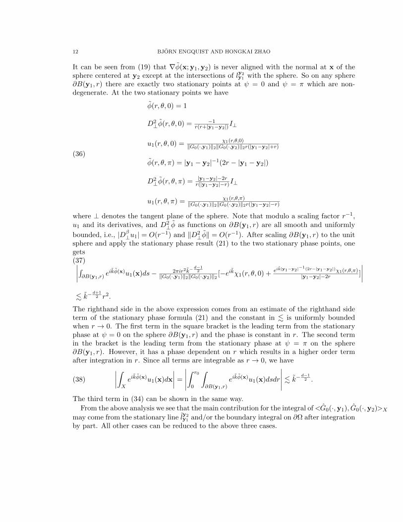
12 BJORN ENGQUIST AND HONGKAI ZHAO
It can be seen from (19) that ∇φ(x; y1,y2) is never aligned with the normal at x of thesphere centered at y2 except at the intersections of ly2
y1 with the sphere. So on any sphere∂B(y1, r) there are exactly two stationary points at ψ = 0 and ψ = π which are non-degenerate. At the two stationary points we have
(36)
φ(r, θ, 0) = 1
D2⊥φ(r, θ, 0) = −1
r(r+|y1−y2|)I⊥
u1(r, θ, 0) = χ1(r,θ,0)‖G0(·,y1)‖2‖G0(·,y2)‖2r(|y1−y2|+r)
φ(r, θ, π) = |y1 − y2|−1(2r − |y1 − y2|)
D2⊥φ(r, θ, π) = |y1−y2|−2r
r(|y1−y2|−r)I⊥
u1(r, θ, π) = χ1(r,θ,π)‖G0(·,y1)‖2‖G0(·,y2)‖2r(|y1−y2|−r)
where ⊥ denotes the tangent plane of the sphere. Note that modulo a scaling factor r−1,u1 and its derivatives, and D2
⊥φ as functions on ∂B(y1, r) are all smooth and uniformly
bounded, i.e., |Dβ⊥u1| = O(r−1) and ‖D2
⊥φ‖ = O(r−1). After scaling ∂B(y1, r) to the unitsphere and apply the stationary phase result (21) to the two stationary phase points, onegets(37)∣∣∣∣∫∂B(y1,r)
eikφ(x)u1(x)ds− 2πir2k−d−12
‖G0(·,y1)‖2‖G0(·,y2)‖2 [−eikχ1(r, θ, 0) + eik|y1−y2|−1(2r−|y1−y2|)χ1(r,θ,π)|y1−y2|−2r ]
∣∣∣∣. k−
d+12 r2.
The righthand side in the above expression comes from an estimate of the righthand sideterm of the stationary phase formula (21) and the constant in . is uniformly boundedwhen r → 0. The first term in the square bracket is the leading term from the stationaryphase at ψ = 0 on the sphere ∂B(y1, r) and the phase is constant in r. The second termin the bracket is the leading term from the stationary phase at ψ = π on the sphere∂B(y1, r). However, it has a phase dependent on r which results in a higher order termafter integration in r. Since all terms are integrable as r → 0, we have
(38)
∣∣∣∣∫Xeikφ(x)u1(x)dx
∣∣∣∣ =
∣∣∣∣∣∫ r0
0
∫∂B(y1,r)
eikφ(x)u1(x)dsdr
∣∣∣∣∣ . k− d−12 .
The third term in (34) can be shown in the same way.
From the above analysis we see that the main contribution for the integral of<G0(·,y1), G0(·,y2)>Xmay come from the stationary line ly2
y1 and/or the boundary integral on ∂Ω after integrationby part. All other cases can be reduced to the above three cases.

APPROXIMATE SEPARABILITY OF GREEN’S FUNCTION FOR HIGH FREQUENCY HELMHOLTZ EQUATIONS13
In 2D, the Green’s function in free space is of the form (10) with the asymptotic formulas(11). For Case 1 and 2, the asymptotic formula (11) for r → ∞ can be used as k → ∞.
Since the phase function in the exponential for < G0(·,y1), G0(·,y2) > is also of the formk(|x−y1|− |x−y2|), same arguments used above can be applied. So we have the followinganalogous results in 2D:
Case 1. Since the boundary ∂X is a one dimensional curve, there is some α, 1 ≤ α ≤d+1
2 = 32 , such that
(39)∣∣∣< G0(·,y1), G0(·,y2) >
∣∣∣ . (k|y1 − y2|)−α, as k|y1 − y2| → ∞
Case 2. The leading contribution is due to the line of stationary phase ly2y1 except that the
dimension orthogonal to the line is 1D, we have d−12 = 1
2 and
(40)∣∣∣< G0(·,y1), G0(·,y2) >
∣∣∣ . (k|y1 − y2|)−12 , as k|y1 − y2| → ∞
Case 3. The singularity at the source is also integrable hence
(41)∣∣∣< G0(·,y1), G0(·,y2) >
∣∣∣ . (k|y1 − y2|)−12 , as k|y1 − y2| → ∞
Here we give a few remarks related to the theorem above.
Remark 2.1. For d = 3, the same estimate also holds for two unnormalized Green’s func-
tions, i.e., |< G0(·,y1), G0(·,y2) >| ∼∣∣∣< G0(·,y1), G0(·,y2) >
∣∣∣, since 0 < c < ‖G0(·,y)‖L2(X) <
C <∞ as k →∞ for two constants c and C that only depend on X. However, this is not
true for d = 2. If y1,y2 /∈ X, |< G0(·,y1), G0(·,y2) >| ∼ k−12
∣∣∣< G0(·,y1), G0(·,y2) >∣∣∣ as
k →∞ due to the asymptotic formula (11).
Remark 2.2. The estimate in Theorem 2.1 characterizes the correlation or angle betweentwo normalized Green’s function in term of the ratio of the separation distance between thetwo sources and the wavelength. One can also incorporate another scaling factor when thedistance from the two points yi, i = 1, 2 to X is large compared to y1−y2|. Geometrically,this means that the difference between two distance functions, |x− y1| − |x− y2|, changesslowly with respect to x ∈ X. Hence fast oscillation due to rapid change of the phasefunction, ik(|x − y1| − |x − y2|) is discounted and the decorrelation rate of two Green’sfunction is reduced.
Assume the size of X is O(1) (otherwise one can first scale x by the size of X for the
Helmholtz equation (5)) and |y1−y2|dist(y1,X) ∼
|y1−y2|dist(y2,X) ∼ ρ 1, which falls into either Case 1
or Case 2 in Theorem 2.1. From (19), we see that ∇φ is scaled by ρ and D2φ,det[D2φ] arescaled by ρ, ρd respectively when they are not degenerate. The scaling for u(x) is canceleddue to the normalization according to the definition (23). When applying the stationary

14 BJORN ENGQUIST AND HONGKAI ZHAO
phase result (21) at a point of stationary phase, one can see that k is rescaled to kρ if
kρ→∞. For Case 1, the main contribution for∣∣∣< G0(·,y1), G0(·,y2) >
∣∣∣ comes from the
last term in (26). There is a scaling factor of ρ−1 from |∇φ|−1 due to the integration by part
and there are isolated stationary points on ∂X in general. So overall k is rescaled to kρ for
Case 1. For Case 2 in Theorem 2.1, the main contribution for∣∣∣< G0(·,y1), G0(·,y2) >
∣∣∣comes from the line of stationary phase in general, where Dφ and D2φ are degenerate.Along the line of stationary phase, D2
⊥φ and det[D2⊥φ] is scaled by ρ2 and ρ2(d−1) respec-
tively from (20). Applying the stationary phase result (21) in the plane perpendicular to
the line of stationary phase, k is rescaled to kρ2. From both cases we see that k is at leastrescaled to kρ in the decorrelation estimate for two Green’s function.
Remark 2.3. One can generalize the arguments in Theorem 2.1 to more general situationswhere X is a compact manifold embedded in Rd with dim(X) = s < d, such as a surface(s = 2) in R3 or a curve (s = 1) in Rd, d = 2, 3. For example, if X is a compact manifoldwithout boundary, e.g., a closed surface or curve, and two points y1,y2 /∈ X, there is someα, 0 ≤ α ≤ s
2
(42)∣∣∣< G0(·,y1), G0(·,y2) >
∣∣∣ . (k|y1 − y2|)−α, as k|y1 − y2| → ∞.
The two extreme cases are: (1) α = 0 happens when there is a piece of X stays on a level
set of the phase function φ(x) = |y1 − y2|−1(|x− y1| − |x− y2|); (2) α = s2 happens if the
phase function φ(x), which has stationary phase points on a compact manifold, has isolated
stationary phase points on X and D2φ(x) is not degenerate along X at those points. Thelater case, α = s
2 , is more generic in practice.
If X is a compact manifold with boundary, there is some α, 0 ≤ α ≤ s+12 such that
(43)∣∣∣< G0(·,y1), G0(·,y2) >
∣∣∣ . (k|y1 − y2|)−α, as k|y1 − y2| → ∞.
The two extreme cases are: (1) α = 0 happens when there is a piece of X stays on a level
set of the phase function φ(x); (2) α = s+12 happens if the phase function φ(x) has no
stationary phase in X and has isolated stationary phase points on ∂X and D2φ(x) is notdegenerate along ∂X at those points. If there are isolated stationary phase points in theinterior of X, α = s
2 .
Remark 2.4. According to the Hessian estimate (20), there are two axisymmetric k de-
pendent domains around the stationary line ly2y1 on each side of y1 and y2, denoted by R1
and R2 respectively (see Figure 4), in which the phase function kφ does not change rapidly.
For example, let’s look at a point x ∈ ly2y1 on the side of y2 and denote r = ±|x − y2|.
Again we use the coordinate system x = (r, ξ, η) as shown in Figure 4. Since φ(r, 0, 0) =
1, |∇φ(r, 0, 0)| = 0, r > 0, for a point (r, ξ, η) with r > 0,√ξ2 + η2 . r(r+|y1−y2|)
k|y1−y2| , from
APPROXIMATE SEPARABILITY OF GREEN’S FUNCTION FOR HIGH FREQUENCY HELMHOLTZ EQUATIONS15
(20) we have
(44) k|∇φ(r, ξ, η)| . k|y1 − y2|√ξ2 + η2
r(r + |y1 − y2|). 1.
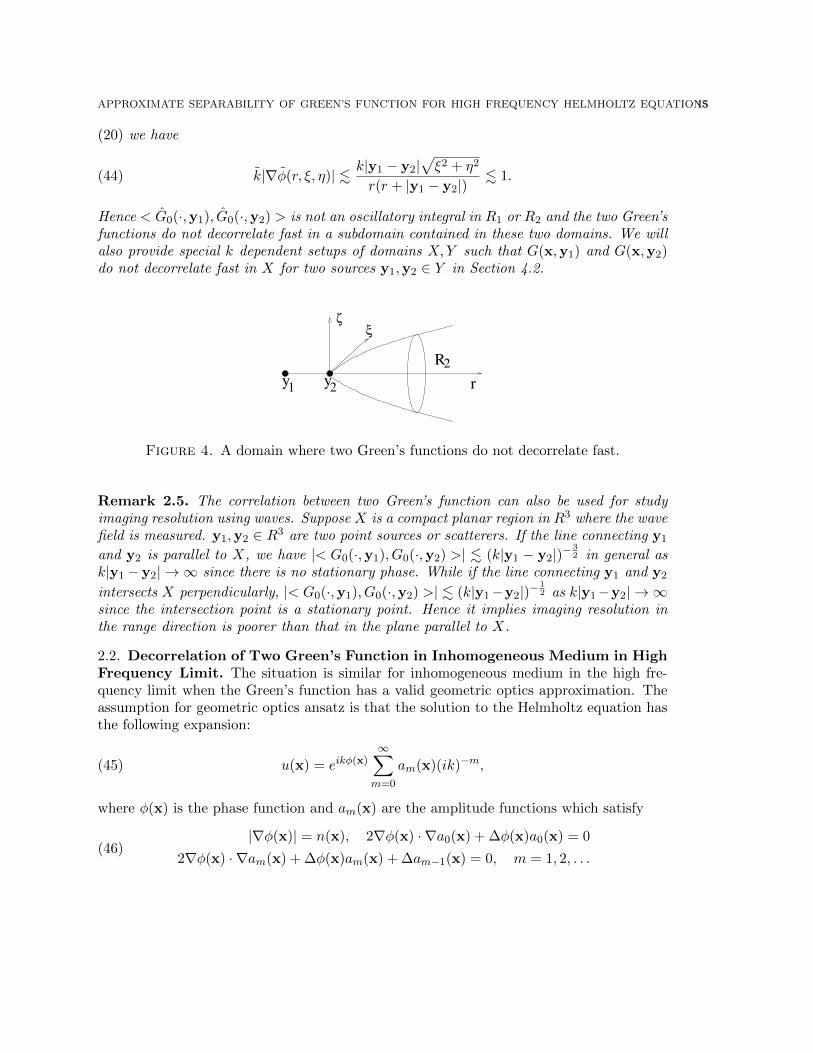
Hence < G0(·,y1), G0(·,y2) > is not an oscillatory integral in R1 or R2 and the two Green’sfunctions do not decorrelate fast in a subdomain contained in these two domains. We willalso provide special k dependent setups of domains X,Y such that G(x,y1) and G(x,y2)do not decorrelate fast in X for two sources y1,y2 ∈ Y in Section 4.2.
2
y1
y2 r
ξζ
R
Figure 4. A domain where two Green’s functions do not decorrelate fast.
Remark 2.5. The correlation between two Green’s function can also be used for studyimaging resolution using waves. Suppose X is a compact planar region in R3 where the wavefield is measured. y1,y2 ∈ R3 are two point sources or scatterers. If the line connecting y1
and y2 is parallel to X, we have |< G0(·,y1), G0(·,y2) >| . (k|y1 − y2|)−32 in general as
k|y1 − y2| → ∞ since there is no stationary phase. While if the line connecting y1 and y2
intersects X perpendicularly, |< G0(·,y1), G0(·,y2) >| . (k|y1−y2|)−12 as k|y1−y2| → ∞
since the intersection point is a stationary point. Hence it implies imaging resolution inthe range direction is poorer than that in the plane parallel to X.
2.2. Decorrelation of Two Green’s Function in Inhomogeneous Medium in HighFrequency Limit. The situation is similar for inhomogeneous medium in the high fre-quency limit when the Green’s function has a valid geometric optics approximation. Theassumption for geometric optics ansatz is that the solution to the Helmholtz equation hasthe following expansion:
(45) u(x) = eikφ(x)∞∑m=0
am(x)(ik)−m,
where φ(x) is the phase function and am(x) are the amplitude functions which satisfy
(46)|∇φ(x)| = n(x), 2∇φ(x) · ∇a0(x) + ∆φ(x)a0(x) = 0
2∇φ(x) · ∇am(x) + ∆φ(x)am(x) + ∆am−1(x) = 0, m = 1, 2, . . .

16 BJORN ENGQUIST AND HONGKAI ZHAO
For the Green’s function G(x,y) defined in (5), we have the following condition at thesource point y:
(47) limx→y
(φ(x,y)
|x− y|− n(y)
)= 0, lim
x→ya0(x,y)4π|x− y| = 1.
The above geometric optics ansatz can be formulated as a Hamiltonian system, alsocalled as Lagrangian formulation or ray tracing, which gives explicit ordinary differen-tial equations (ODE) for bicharacteristics (x(t),p(t)) in phase space with HamiltonianH(x,p) = |p| − n(x) and p = ∇φ,
(48)
dx(t,x0,p0)
dt= ∇pH(x,p) =
p
n(x), x(0) = x0,
dp(t,x0,p0)
dt= −∇xH(x,p) = ∇n(x), p(0) = p0 = ∇φ(x0)
dφ(x(t,x0,p0))
dt= ∇φ · dx
dt= n(x), φ(0) = φ(x0)
The projection of the bicharacteristics in the physical space, i.e., x(t,y0,p0), are calledrays. If there is no caustics, i.e., two rays do not intersect in the physical space, each rayis a geodesic in the physical space with the slowness n(x) = 1
c(x) as the metric, where c(x)
is the wave speed. |φ(x(t2,x0,p0)) − φ(x(t1,x0,p0))| is the shortest travel time betweenpoints x(t1,x0,p0) and x(t2,x0,p0). Moreover, the amplitude along each ray is given by
(49) a20(x(t,x0)) = a2
0(x0)n(x0)
n(x(t,x0))
∣∣∣∣∂x(t,x0)
∂x0
∣∣∣∣−1
,
where∣∣∣∂x(t,x0)
∂x0
∣∣∣ is the determinant of the Jacobian ∂x(t,x0)∂x0
meaning the geometric spreading
of rays. Before caustics are formed, the determinant is always positive and bounded. Oncea0(x) is known, a1(x), a2(x), . . . can be solved consecutively from (46).
In particular, for the geometric optics ansatz for the Green’s function with a pointsource at y0, rays x(t,y0, θ) are emanating from the source y0 in all directions and can
be parametrized by the initial directions, i.e., the take-off angles θ ∈ Sd−1 on a unitsphere. The ODEs for the rays (48) have initial conditions x(0,y0, θ) = y0,p(0,y0, θ) =
n(y0)θ, φ(0,y0, θ) = 0, with a0(0, θ) evenly distributed in all θ. If there is no caus-
tics, every point x has a unique ray passing through it, i.e., ∀x, ∃!t(x), θ(x) such that
x(t(x),y0, θ(x)) = x. Moreover, the ray connecting y0 and x is the geodesic, or the short-est travel time, between the two points with n(x) being the slowness of the medium. Underno caustics assumptions, the Greens functions with sources at y1,y2 can be approximatedby the following geometric optics ansatz
(50)∣∣∣G(x,yj)− eikφ(x,yj)Aj(x)
∣∣∣ . k−(M+1), j = 1, 2,

APPROXIMATE SEPARABILITY OF GREEN’S FUNCTION FOR HIGH FREQUENCY HELMHOLTZ EQUATIONS17
where Aj(x) =∑M
m=0 am(x,yj)(ik)−m, j = 1, 2. Hence
(51)
∣∣∣∣< G(·,y1), G(·,y2) > −∫Xeikφ(x)u(x)dx
∣∣∣∣ . k−(M+1),
where
k = kφ(y1,y2), φ(x) = φ−1(y1,y2)(φ(x,y1)−φ(x,y2)), u(x) =A1(x)A2(x)
‖G(·,y1)‖2‖G(·,y2)‖2
Denote Γy2y1 to be the unique ray that passes through y1 and y2 as illustrated in Figure 5
(a). If n(x) is smooth and 0 < c ≤ n(x) ≤ C <∞, one has (see Figure 5(b))
c|y1 − y2| ≤ φ(y1,y2) ≤ C|y1 − y2|, |φ(x,y1)− φ(x,y2)| ≤ φ(y2,y1)
So the phase function φ(x) attains the global maximum or minimum ±1 on the part of
the ray Γy2y1 which is outside the interval between y1 and y2, denoted by Γy2
y1 . Moreover,
∇xφ(x,y1) − ∇xφ(x,y2) 6= 0 for any x that is not on Γy2y1 because the two different and
unique geodesics connecting x,y1 and x,y2 respectively can not be tangent at x . So Γy2y1
is a stationary curve in the inhomogeneous case and plays the same role as the straightline ly2
y1 in the homogeneous case. Depending on whether the ray passes through X or not,we get the same results as in Theorem 2.1 because kφ(y1,y2) ∼ k|y1 − y2|. This is truewhen y1 and/or y2 are in X as well since the amplitude a0 satisfying (47) has exactly thesame singularity as the homogeneous Green’s function.
The main complication for geometric optics ansatz in heterogeneous medium is whenrays cross each other, i.e., when caustics are formed. Although bicharacteristics in phasespace are still well defined, the amplitude formula (49) breaks down. So in general, theabove arguments can not be carried over to a general inhomogeneous medium. However, inthe case that there are finite number of rays starting from y1 going through y2 and there isa partition of unity for the takeoff angle θ on Sd−1 such that there is a small cone aroundeach ray where there is no caustics, then one can apply the above argument to each coneand get the same results.
ray
y1 y
2
X
y1
Γy
2
)y1 y
2
X
xφ(x,y1
)
φ(y φ(x,y2
)1,y
2
(a) (b)
Figure 5. Rays in inhomogeneous medium

18 BJORN ENGQUIST AND HONGKAI ZHAO
3. Approximate Separability Estimate for the Green’s function ofHelmholtz equation in High Frequency Limit
In this section we present general estimates for the approximate separability of Green’sfunction of Helmholtz equation in the high frequency limit. In the next section, we willapply these results to get explicit estimates for special setups that are of interest in practice.These estimates imply rank estimates for discretized operators which are important fordeveloping fast algorithms for solving high frequency Helmholtz equation and its boundaryintegral equation counterpart.
3.1. Approximating a Set of Almost Orthogonal Vectors by a Linear Subspace.First we present some background and introduce definitions for the approximation of a setof vectors using a linear subspace. It will be extended later to the approximation of Green’sfunction in the infinite dimensional function space. Let vm ∈ Rd,m = 1, 2, . . . , N be a setof vectors. Define matrix V = [v1,v2, . . . ,vN ] and matrix A = [amn]N×N = V TV . Let
λ1 ≥ λ2 ≥ . . . ≥ λN ≥ 0 be the eigenvalues of A, then tr(A) =∑N
m=1 λm =∑N
m ‖vm‖22.√λ1 ≥
√λ2 ≥ . . . ≥
√λN ≥ 0 are also called singular values for V . The best linear
subspace Sl of all linear subspace Sl of dimension l that approximates the set of vectorsvmNm=1 in least square sense is the space spanned by the first l left singular vectors of Vand satisfies
(52)
N∑m
‖vm − PSlvm‖22 = min
Sl,dim(S)=l
N∑m
‖vm − PSlvm‖22 =
N∑m=l+1
λm,
where PSlv denotes projection of v in Sl. In another word,
(53) λl = maxe∈Rd,‖e‖2=1,e⊥Sl−1
N∑j
|vj · e|2,
is the maximum reduction of approximation error in term of least square for the set ofvectors vmNm=1 when adding one more dimension to the previous optimal l−1 dimensionallinear subspace. Here we introduce two definitions for approximate rank estimate for asymmetric non-negative matrix A.
Definition 3.1. Given ε > 0, Nε
= max1≤m≤N m, s.t.√λm ≥ ε, i.e.,N
εdenotes the
largest m such that√λm ≥ ε.
Definition 3.2. Given 1 ≥ ε > 0, N ε = minM, s.t.∑N
m=M+1 λm ≤ ε2∑N
m=1 λm.
If A = V TV , definition 3.2 implies that if a linear subspace Sε satisfies
(54)
∑Nm=1 ‖vm − PSεvm‖22∑N
m=1 ‖vm‖22≤ ε2

APPROXIMATE SEPARABILITY OF GREEN’S FUNCTION FOR HIGH FREQUENCY HELMHOLTZ EQUATIONS19
then dim(Sε) ≥ N ε. Assume 0 < c < ‖vm‖2 < C < ∞,m = 1, 2, . . . , N , we can concludethat if a linear subspace Sε satisfies
(55)
√∑Nm=1 ‖vm − PSεvm‖22
N≤ cε ⇒
∑Nm ‖vm − PSεvm‖22∑N
m=1 ‖vm‖22≤ ε2
then dim(Sε) ≥ N ε. In another word, the least dimension of a linear subspace that can havean cε-r.m.s. (root mean square) approximation of a set of vectors vm,m = 1, 2, . . . , N isat least N ε. The root mean square approximation will lead to L2 approximate separabilityestimate for Green’s function in the continuous case.
In the previous section, we proved the rate of decorrelation of two Green’s function: | <G(·,y1), G(·,y1) > | . (k|y1−y2|)−α for some α > 0 as k|y1−y2| → ∞. Geometrically itmeans that two Green’s functions with sources separated a little more than one wavelengthbecome almost orthogonal as k →∞. Intuitively, for two domains X,Y ⊂ Rd, if one viewsG(x,y) as a family of functions in L2(X) parametrized by y ∈ Y and lays downs a uniformgrid yj ∈ Y with grid size h = k−β for any 0 < β < 1, G(x,yj) is a set of almost orthogonalvectors in L2(X). A natural question is the least number of dimensions of a linear spacethat can contain a set of almost orthogonal vectors. This question has been studied in [1] byrank estimate for small off-diagonal perturbation of identity matrices, which is equivalent tothe same question for a set of almost orthogonal unit vectors. In particular, the asymptoticestimate is optimal and is used to show the sharpness of Johnson-Lindenstraus Lemma [19].However, this result can not address our problem adequately for the following two reasons.First, the assumption in [1] on almost orthogonality for a set vectors is only pairwise.In our problems, the set of vectors are Green’s functions for a PDE which has spatialstructure, i.e., the angle between two Green’s functions depends on separation distance ofthe two sources. The spatial structure has to be taken into account to get sharp estimates.Second, approximate separability means that we need to estimate the least dimension ofa linear subspace that can approximate a set of vectors to a certain tolerance instead ofcontaining the whole set of vectors. Here we adopt the approach from [1] and developmore careful estimates in Lemma 3.1 for a set of Green’s functions by taking into accountboth the spatial structure and approximation tolerance. The lemma is then used to provelower bound estimates for approximate separability of the Green’s function for Helmholtzequation in the high frequency limit.
For more generality, we assume X,Y are two compact manifolds embedded in Rd, i.e.,they may be compact domains in Rd, or compact surfaces embedded in R3 or compactcurves embedded in Rd, d = 2 or 3. Without loss of generality, we assume d ≥ dim(X) ≥dim(Y ) = s. For a smooth manifold Y with dim(Y ) = s = 1, 2, 3, it contains a localpatch of size O(1) that is diffeomorphism to a one dimensional line of unit length, a twodimensional unit square and a three dimensional unit cube respectively, which we will onlyconsider in the following analysis. Let G(x,y) be the Green’s function of the Helmholtzequation (5). The following Lemma 3.1 shows the dimension estimate for a linear subspacein L2(X) which approximate of a set of Green’s function G(x,ym),ym ∈ Y with ε-r.m.serror.

20 BJORN ENGQUIST AND HONGKAI ZHAO
Lemma 3.1. Let X,Y be two compact manifolds embedded in Rd, d = 2, 3 and d ≥dim(X) ≥ dim(Y ) = s. If for any two points y1,y2 ∈ Y ,
| < G(·,y1), G(·,y2) > | . (k|y1 − y2|)−α as k|y1 − y2| → ∞
for some α > 0, then there are points ym ∈ Y,m = 1, 2, . . . , N sδ ∼ ks−δ, for any 0 < δ < 1
and arbitrary close to 0, such that for the set of Green’s functions G(x,ym)Nsδ
m=1 ⊂ L2(X)
and matrix A =< G(·,ym), G(·,yn) >
(56) N εk &
(1− ε2)2k2α, α < s
2 ,
(1− ε2)2ks−δ, α ≥ s2 ,
and
(57) Nεk .
ε−4k2(s−α−δ), α < s2 ,
ε−4ks−δ, α ≥ s2 ,
as k →∞, where the constants in . and & only depend on X, Y and n(x).
Proof. We prove the statement for X,Y ⊂ R3 and dim(Y ) = s = 1, 2, 3 respectively. Thecase for X,Y ⊂ R2 can be proved in exactly the same way.
Case 1: s = 1. Y is a line of unit length in R3. Put down a uniform grid ym in Y withgrid size h = kδ−1, 0 < δ < 1, such that |ym− yn| ∼ |m− n|h, m, n = 1, 2, . . . , nhk = k1−δ.See Figure 6(a). Define the matrix
(58) A = (amn)nhk×nhk, amn =< G(·,ym), G(·,yn) >,
where
(59) amm = 1, |amn| . |m− n|−αk−αδ, m, n = 1, 2, . . . , nhk .
Let λ1 ≥ λ2 ≥ . . . ≥ λnhk≥ 0 be the eigenvalues of A. Then
∑nhkm=1 λm = nhk . Since N
εk =
max1≤m≤nhkm, s.t.
√λm ≥ ε and N ε
k = minM, s.t.∑nhk
m=M+1 λm ≤ ε2∑nhk
m=1 λm = ε2nhk ,
we haveNεk∑
m=1
λm ≥ (1− ε2)
nhk∑m=1
λm = (1− ε2)nhk
and
(60)
nhk∑m=1
λ2m >
Nεk∑
m=1
λ2m ≥ N ε
k
[(1− ε2)nhk
N εk
]2
=[(1− ε2)nhk ]2
N εk
,
and
(61)
nhk∑m=1
λ2m >
Nεk∑
m=1
λ2m ≥ N
εkε
4.

APPROXIMATE SEPARABILITY OF GREEN’S FUNCTION FOR HIGH FREQUENCY HELMHOLTZ EQUATIONS21
At the same time, for a fixed α > 0 and take 0 < δ < 1 arbitrary close to 0,
(62)
∑nhkm=1 λ
2m = tr(ATA) =
∑nhkm=1
∑nhkn=1 a
2mn
=∑nhk
m=1 a2mm + 2
∑nhk−1n=1
∑nhkm=n+1 a
2m,m−n
. nhk + 2∑nhk−1
n=1 (nhk − n)n−2αk−2αδ
.
k1−δ + k2(1−δ−α) . k2(1−δ−α), α < 1
2 , 2α < 1− δ < 1
k1−δ + k1−2δ ln k . k1−δ, α = 12 , 0 < δ < 1
k1−δ + k1−δ−2αδ . k1−δ, α > 12 , 0 < δ < 1
Hence for a fixed α > 0 and any 0 < δ < 1 arbitrary close to 0, combining (60) and (62)we have
(63) N εk &
(1− ε2)2k2α, α < 12
(1− ε2)2k1−δ, α ≥ 12
,
and combining (61) and (62) we have
(64) Nεk .
ε−4k2(1−α−δ), α < 12
ε−4k1−δ, α ≥ 12
.
Case 2: s = 2. Y is a unit square in R3. Again put down a uniform grid ym,m =1, 2, . . . , nhk = k2(1−δ) in Y with grid size h = kδ−1, 0 < δ < 1 (see Figure 6(b)), and define
matrix A as in (58). Let λ1 ≥ λ2 ≥ . . . ≥ λnhk≥ 0 be its eigenvalues, then
∑nhkm=1 λm = nhk
and we have (60), (61). At the same time
(65)
nhk∑m=1
λ2m = tr(ATA) =
nhk∑m=1
nhk∑n=1
a2mn.
Let’s look at the sum of each row. Assume ym is the center of the square. We divide allother points into groups of 1st square neighbors, 2nd square neighbors, . . ., j-th squareneighbors, denoted by Sj , j = 1, 2, . . . , J ∼ h−1 = k1−δ. See Figure 6(b). Sj contains those4(2j + 1) − 4 = 8j grid points that are on the 4 sides of the square centered at ym witheach side of length 2jh. Then we have jh ≤ |ynj − ym| ≤
√2jh,ynj ∈ Sj , and hence
am,nj . (kjh)−α = j−αk−αδ. For a fixed α > 0 and take 0 < δ < 1 arbitrary close to 0, we

22 BJORN ENGQUIST AND HONGKAI ZHAO
have
(66)
∑nhkn=1 a
2mn = 1 +
∑Jj=1
∑nj∈Sj a
2m,nj . 1 +
∑Jj=1 j
−2α+1k−2αδ
.
1 + k2(1−δ−α) . k2(1−δ−α), α < 1, α < 1− δ < 1
1 + k−2δ ln k . 1, α = 1, 0 < δ < 1
1 + k−2αδ . 1, α > 1, 0 < δ < 1
Actually for any grid point ym, each j-th square neighbors of ym has at least 8j/4 = 2jpoints for j = 1, 2, . . . , J ∼ k1−δ, e.g., if ym is a corner point of the square domain. Hencethe above asymptotic formula is still true. For a fixed α > 0 and any 0 < δ < 1 arbitraryclose to 0, we have
(67)
nεk∑m=1
λ2m ≤
nhk∑m=1
nhk∑n=1
a2mn .
k2(2(1−δ)−α), α < 1
k2(1−δ), α ≥ 1
Combining (67) with (60), we have
(68) N εk &
(1− ε2)2k2α, α < 1
(1− ε2)2k2(1−δ), α ≥ 1..
Combining (67) with (61), we have
(69) Nεk .
ε−4k2(2(1−δ)−α), α < 1
ε−4k2(1−δ), α ≥ 1
.
m
Y
y1
y2
y
Y
ym
S1
S2
(a) (b)
Figure 6. Green’s functions with sources on a uniform grid.

APPROXIMATE SEPARABILITY OF GREEN’S FUNCTION FOR HIGH FREQUENCY HELMHOLTZ EQUATIONS23
Case 3: s = 3. Y is a unit cube in R3. Put down a uniform grid ym,m = 1, 2, . . . , nhk =
k3(1−δ) in Y with grid size h = kδ−1, 0 < δ < 1 and define matrix A as in (58). Let
λ1 ≥ λ2 ≥ . . . ≥ λnhk≥ 0 be its eigenvalues, then
∑nhkm=1 λm = nhk and we have (60),
(61). Similar to 2D case, assume ym is the center of the cube. We divide all other pointsinto groups of 1st cube neighbors, 2nd cube neighbors, . . ., j-th cube neighbors, denoted byCj , j = 1, 2, . . . , J ∼ h−1 = k1−δ. Cj contains those 6(2j+1)2−12(2j+1)+8 = 24j2+2 gridpoints ynj that are on the faces of the cube centered at ym with each face a square of length
2jh. Then we have jh ≤ |ynj − ym| ≤√
3jh,ynj ∈ Cj , and am,nj . (kjh)−α = j−αk−αδ.For 0 < δ < 1 arbitrary close to 0, one has the row sum estimate
(70)
∑nhkn=1 a
2mn = 1 +
∑Jj=1
∑nj∈Cj a
2m,nj . 1 +
∑Jj=1(24j2 + 2)j−2αk−2αδ
.
1 + k3(1−δ)−2α . k3(1−δ)−2α, α < 3
2 ,23α < 1− δ < 1
1 + k−3δ ln k . 1, α = 32 , 0 < δ < 1
1 + k−2αδ . 1, α > 32 , 0 < δ < 1.
Also this is true for any point ym which has at least 1/8 of 24j2 + 2 points in its j-thcube neighbor Cj for j = 1, 2, . . . , J ∼ k1−δ. Hence for a fixed α > 0 and any 0 < δ < 1arbitrary close to 0,
(71)
nεk∑m=1
λ2m ≤
nhk∑m=1
nhk∑n=1
a2mn .
k2(3(1−δ)−α), α < 32
k3(1−δ), α ≥ 32
Combining (71) with (60), we have
(72) N εk &
(1− ε2)2k2α, α < 3
2
(1− ε2)2k3(1−δ), α ≥ 32
.
Combine (71) with (61), we have
(73) Nεk .
ε−4k2(3(1−δ)−α), α < 32
ε−4k3(1−δ), α ≥ 32
.
Replace sδ by δ in each of the above cases, we complete the proof.
Remark 3.1. When d = 3, if either dim(X) = dim(Y ) = 3 or X and Y are separated,there are 0 < c < c < ∞ independent of k such that c ≤ ‖G(·,y)‖2 ≤ c uniformlyin y ∈ Y . For the same set of Green’s functions G(x,yj) as in the above proof andA =< G(·,ym), G(·,yn) >, we have
(74) cnhk ≤nhk∑m=1
λm ≤ cnhk ⇒Nεk∑
m=1
λm ≥ (1− ε2)
nhk∑m=1
λm ≥ (1− ε2)cnhk .

24 BJORN ENGQUIST AND HONGKAI ZHAO
Hence inequalities (60) is replaced by the following:
(75)
nhk∑m=1
λ2m >
Nεk∑
m=1
λ2m ≥ N ε
k
[(1− ε2)cnhk
N εk
]2
=[(1− ε2)cnhk ]2
N εk
,
and (61) is the same. The estimate of∑nεk
m=1 λ2m ≤
∑nhkm=1
∑nhkn=1 a
2mn is amplified by c2
from the previous estimate at most. So the same results are true.
When d = 2, except for a scaling factor k−12 for the Green’s function, everything else is
similar to the case d = 3. By the definition 3.2 of N εk, it is independent of a constant scaling
of the whole set of vectors. So the results for N εk also holds for A =< G(·,ym), G(·,yn) >.
Remark 3.2. The size of Y can be scaled for the result of Lemma 3.1. If α ≥ s2 , trace
estimates (62), (67), and (71) gives∑nhk
m=1 λ2m . nhk. It can be seen easily from (60) and
(61) that if Y is scaled to aY , k is scaled to ak in those estimates (56), (57) for N εk and
Nεk respectively. Otherwise, the only factor that can not be scaled with nhk in the trace
estimates is k−2αδ in (62), (66) and (70). Hence, in addition to scale k to ak, there is anextra factor of a2αδ for the result of Lemma 3.1.
Remark 3.3. The key estimates in the proof of Lemma 3.1 are (60) (or (75)), (61), and
the one for∑nhk
m=1 λ2m = tr(ATA). Although the estimate of tr(ATA) can be improved by
more careful estimates of each row sum∑nhk
n=1 a2mn by taking into account different decorre-
lation rate according to Theorem 2.1, e.g., dividing those points in each j-th square (cube)neighbors of ym (see Figure 6) into directional cone sections according to whether the lineconnecting ym and its neighbors intersecting X or not, which gives different decorrelationrate of two Green’s functions or different power α in am,nj . (kjh)−α for points in differentcones, as long as there is a solid angle cone such that lines connecting those neighbors inthat section and ym intersect X, the order of the estimate can not be improved. On theother hand, whether (60) and (61) are sharp or not is a more complicated issue. The answer
depends on the variation of leading eigenvalues of the matrix A =< G(·,ym), G(·,yn) >,which depends on the geometric setup of X and Y , and the choice of ε.
3.2. Lower Bound and Upper Bound Estimate for Approximate Separability ofGreen’s Function. Now we use Lemma 3.1 to prove the following lower bound estimatefor approximate separability (14) of Green’s function for Helmholtz equation (5) in thehigh frequency limit.
Theorem 3.1. Let X,Y be two compact manifolds embedded in Rd, d = 2, 3, and d ≥dim(X) ≥ dim(Y ) = s. Assume that for any two points y1,y2 ∈ Y ,
| < G(·,y1), G(·,y2) > | . (k|y1 − y2|)−α as k|y1 − y2| → ∞

APPROXIMATE SEPARABILITY OF GREEN’S FUNCTION FOR HIGH FREQUENCY HELMHOLTZ EQUATIONS25
for some α > 0. If there are fl(x) ∈ L2(X), gl(y) ∈ L2(Y ), l = 1, 2, . . . , N εk such that
(76)
∥∥∥∥∥∥G(x,y)−Nεk∑
l=1
fl(x)gl(y)
∥∥∥∥∥∥L2(X×Y )
≤ ε,
then
(77) N εk ≥
cεk
2α, α < s2 ,
cεks−δ, α ≥ s
2 ,
for any 0 < δ < 1 and arbitrary close to 0 as k → ∞, where cε ≥ c(1 − (Cε)2)2 for somepositive constants c and C that only depend on X, Y and n(x).
Proof. Without loss of generality, we assume Y is a line of unit length, a unit square ora unit cube for s = 1, 2, 3 respectively. First, put down a uniform coarse grid in Y withgrid size h = kδ−1, 0 < δ < 1 and is arbitrary close to 0. The grid divides Y into cells
Ym,m = 1, 2, . . . Nhk = ks(1−δ). Divide each coarse cell Ym further into uniform finer cells
of size h < k−1, Ym,n, n = 1, 2, . . . , Nhk = (h/h)s. See Figure 7. For a fixed n, Ym,n is in
the same relative location in each coarse cell Ym. The center and volume of each cell Ym,nis ym,n and hs respectively. Define Gh(x,y) = G(x,ym,n),∀y ∈ Ym,n to be a piecewise
constant function in y. We show that by choosing h < k−1 small enough
(78)
∫Ydy
∫X|G(x,y)−Gh(x,y)|2dx =
Nhk∑
m=1
Nhk∑
n=1
∫Ym,n
dy
∫X|G(x,y)−G(x,ym,n)|2dx . ε2
If X,Y are disjoint, assuming n(x) is smooth in the Helmholtz equation (5) and there is no
caustics, we have |∇yG(x,y)| . k uniformly in x ∈ X and y ∈ Y . One can pick h < k−1
small enough such that
|G(x,y)− G(x,ym,n)| ≤ ε, ∀x ∈ X,y ∈ Ym,n, m = 1, 2, . . . , Nhk , n = 1, 2, . . . , N
hk .
and get (78).
m,n
Ω
ΩY
mΩY
Ym,n
y
Figure 7. Two scale decomposition of the source domain.

26 BJORN ENGQUIST AND HONGKAI ZHAO
If X and Y are not disjoint and dim(X) = dim(Y ) = d = 2 or 3, G(·,y) ∈ L2(X), ∀y ∈Y , we show that there is still h < k−1 small enough such that
(79)
∫X|G(x,y)− G(x,ym,n)|2dx . ε2, ∀y ∈ Ym,n,
which implies (78). From (12) and the asymptotic formulas (7), (8), we have
(80)
∫Bτ (y)
|G(x,y)|2dx . τ
with the constant independent of k, where Bτ (y) denotes the ball with radius τ centeredat y. Hence there are balls Bτ(ε)(y) and Bτ(ε)(ym,n) with radius τ(ε) ∼ ε2 such that
(81)
∫X∩Bτ(ε)(y)
|G(x,y)|2dx ≤ ε2,∫X∩Bτ(ε)(ym,n)
|G(x,ym,n)|2dx ≤ ε2
for a given ε, Denote Xε = X ∩ (Bτ(ε)(y) ∪ Bτ(ε)(ym,n)) and XCε = X \Xε. For y ∈ Ym,n
we have∫X |G(x,y)− G(x,ym,n)|2dx
=∫XCε|G(x,y)− G(x,ym,n)|2dx +
∫Xε|G(x,y)− G(x,ym,n)|2dx = I + II
Since |∇yG(x,y)| . max(kτ−1(ε), τ−2(ε)), ∀x ∈ XCε , by choosing h < k−1 small enough
we get I . ε2. From (81) we get II . ε2. Hence we prove (79).
Let the linear subspace SX = spanfp(x)Nεk
p=1 ⊂ L2(X), then∫Y‖G(x,y)− PSX G(x,y)‖2L2(X)dy ≤ ε
2,
where PSX is the projection onto SX . From (78), we have∫Y‖(I − PSX )[G(x,y)− Gh(x,y)]‖2L2(X)dy . O(ε2),
where I is the identity map, from (78) we have
(82)
ε2 &∫Y ‖(I − PSX )Gh(x,y)]‖2L2(X)dy
=∑Nh
km=1
∑Nhk
n=1
∫Ym,n‖(I − PSX )G(x,ym,n)‖2L2(X)dy
= hs∑Nh
km=1
∑Nhk
n=1 ‖G(x,ym,n)− PSX G(x,ym,n)‖2L2(X)
= (h/h)shs∑Nh
km=1
∑Nhk
n=1 ‖G(x,ym,n)− PSX G(x,ym,n)‖2L2(X)
& 1
Nhk
∑Nhk
n=11
Nhk
∑Nhk
m=1 ‖G(x,ym,n)− PSX G(x,ym,n)‖2L2(X)

APPROXIMATE SEPARABILITY OF GREEN’S FUNCTION FOR HIGH FREQUENCY HELMHOLTZ EQUATIONS27
Assume(83)Nhk∑
m=1
‖G(x,ym,n)− PSX G(x,ym,n)‖2L2(X) = minn
Nhk∑
m=1
‖G(x,ym,n)− PSX G(x,ym,n)‖2L2(X)
Then there is a constant C > 0 such that
(84)1
Nhk
Nhk∑
m=1
‖G(x,ym,n)− PSX G(x,ym,n)‖2L2(X) ≤ C2ε2
Since ym,n ∈ Y,m = 1, 2, . . . Nhk = ks(1−δ) forms a uniform grid with grid size h = kδ−1, we
can apply Lemma 3.1 to get
dim(SX) ≥
c(1− (Cε)2)2k2α α < s
2
c(1− (Cε)2)2ks−δ α ≥ s2
for any 0 < δ < 1 and arbitrary close to 0 as k → ∞, where C > 0, c > 0 are someconstants that depend only on X and Y and n(x).
Remark 3.4. Theorem 3.1 presents the intrinsic mathematical difficulty for numericalcomputation of Helmholtz equation with large wave number k. When n = 3, the same lowerbound estimate for approximate separability holds for unnormalized Green’s function too.Hence, a discretized system, such as the discretized kernel in boundary integral formulationor inverse of the matrix corresponding to direct discretization of the PDE and its off-diagonal sub-matrices corresponding to a mesh that resolves the wavelength, does not havelow rank approximation for large k due to the decorrelation of Green’s functions caused by
fast oscillations. However, when n = 2, for separated X and Y , |G(x,y)| . k−12 ,∀(x,y) ∈
X × Y which approximate separability trivial when k is large enough.
Remark 3.5. Although it seems that the lower bound estimate (77) in Theorem 3.1 showsa weak dependence of N ε
k on ε as k → ∞, the choice of ε can affect the sharpness of thelower bound as commented in Remark 3.3.
Here we also give an upper bound estimate for the approximate separability of Green’sfunction in the high frequency limit. The intuition is that the Green’s functions withsources located within a wavelength are correlated. So use the linear subspace spanned byGreen’s functions sampled uniformly in the source domain with a grid size smaller thanwavelength should approximate the whole family of Green’s functions good enough.
Theorem 3.2. Let X,Y be two compact manifolds embedded in Rd, d = 2, 3 and d ≥dim(X) ≥ dim(Y ) = s. For any ε > 0 and δ > 0, there are fl(x) ∈ L2(X), gl(y) ∈
28 BJORN ENGQUIST AND HONGKAI ZHAO
L2(Y ), l = 1, 2, . . . , N εk ≤ Cks+δ such that
(85)
∥∥∥∥∥∥G(x,y)−Nεk∑
l=1
fl(x)gl(y)
∥∥∥∥∥∥L2(X×Y )
≤ ε
as k →∞, where C > 0 is some constant that depends on X, Y and n(x).
Proof. Put down a uniform grid in Y , which is assumed to be a line of unit length, aunit square or a unit cube for s = 1, 2, 3 respectively, with grid size h = k−1−δ/2. Denotethe grid point as ym,m = 1, 2, . . . , Nh
k = ks(1+δ/2). Denote the liner subspace SX =
spanG(x,ym)Nhk
m=1 ⊂ L2(X). We claim
(86) ‖G(x,y)− PSX G(x,y)‖L2(X) ≤ |Y |−12 ε
for k large enough, where |Y | denotes the volume of Y .If X and Y are disjoint, assuming n(x) is smooth in the Helmholtz equation (5) and
there is no caustics, we have |∇yG(x,y)| . k, ‖D2yG(x,y)‖ . k2, where the bound is
uniform in X and Y . Given a non-grid point y ∈ Y , G(x,y) can be approximated by alinear interpolation, which is convex combination of Green’s function at its neighboringgrid points. To be precise, suppose y ∈ Y lies in the s dimensional simplex with verticesym1 , . . . ,yms+1 . Let r1
y, . . . , rs+1y be the barycentric coordinates for y, i.e.,
y =
s+1∑j=1
rjyymj , 1 ≥ rjy ≥ 0,
s+1∑j=1
rjy = 1.
Then we have the following linear interpolation
(87) |G(x,y)−s+1∑j=1
rjyG(x,ymj )| . ‖D2yG(x,y)‖h2 . k−δ,
and hence (86) is true when k is large enough.
If X and Y are not disjoint and dim(X) = dim(Y ) = d = 2, 3, G(·,y) ∈ L2(X). For agiven ε, there are balls Bτ(ε)(y) and Bτ(ε)(ymj ) with radius 0 < τ(ε) ∼ ε2 centered at yand ymj , j = 1, 2, . . . , d+ 1 such that
(88)
∫Bτ(ε)(y)
|G(x,y)|2dx ≤ ε2
8|Y |(d+ 2),
∫Bτ(ε)(ymj )
|G(x,ymj )|2dx ≤ε2
8|Y |(d+ 2).
Also we have |∇yG(x,y)| . max(kτ−1(ε), τ−2(ε)), ‖D2yG(x,y)‖ . max(k2τ−1(ε), kτ−2(ε), τ−3(ε))
and hence(89)
|G(x,y)−s+1∑j=1
rjyG(x,ymj )| . ‖D2yG(x,y)‖h2 . max(k2(1−γ), k1−2γτ−2(ε), k−2γτ−3(ε)).

APPROXIMATE SEPARABILITY OF GREEN’S FUNCTION FOR HIGH FREQUENCY HELMHOLTZ EQUATIONS29
for any x ∈ X \ Bτ(ε)(y) ∪ (∪d+1j=1Bτ(ε)(ymj )). By decomposing the integration in (86)
on X into two parts, one on Xε = X ∩ (Bτ(ε)(y) ∪ (∪d+1j=1Bτ(ε)(ymj ))) and the other on
XCε = X \ (Bτ(ε)(y) ∪ (∪d+1
j=1Bτ(ε)(ymj ))), we have
(90)
∫Xε|G(x,y)−
∑d+1j=1 r
jyG(x,ymj )|2dx
≤ 2∫Xε|G(x,y)|2 +
∑d+1j=1 r
jy|G(x,ymj )|2dx
≤ 2∫Bτ(ε)(y)∪(∪d+1
j=1Bτ(ε)(ymj )) |G(x,y)|2 +∑d+1
j=1 rjy|G(x,ymj )|2dx
≤ ε2
2|Y | ,
and from (89)
(91)
∫XCε
|G(x,y)−d+1∑j=1
rjyG(x,ymj )|2dx ≤ε2
2|Y |
when k is large enough. Combining the above two parts we get (86) when k is large enough,which implies
(92)
√∫Y‖G(x,y)− PSX G(x,y)‖2L2(X)dy ≤ ε.
Remark 3.6. The above upper bound holds for unnormalized Green’s function when d = 3.
If dim(X) = dim(Y ) = d = 2, 3, since the Green’s function belongs to L2(X × Y ),our approximate separability estimates in L2 norm is valid for general compact domainsX and Y , disjoint or not. However, if X and Y are disjoint, which is the case for mostapplications, our results in L2 norm are also true in L∞(X × Y ) norm. Since L∞ norm isstronger than L2 norm in a compact domain, the lower bound for approximate separabilityin Theorem 3.1 immediately extends to L∞ norm. Also, first part of the proof in Theorem3.2 directly extends to L∞ norm. We summarize these two results below.
Theorem 3.3. Let X,Y be two disjoint compact manifolds embedded in Rd, d = 2, 3, andd ≥ dim(X) ≥ dim(Y ) = s. Assume that for any two points y1,y2 ∈ Y ,
| < G(·,y1), G(·,y2) > | . (k|y1 − y2|)−α as k|y1 − y2| → ∞
for some α > 0. If there are fl(x) ∈ L∞(X), gl(y) ∈ L∞(Y ), l = 1, 2, . . . , N εk such that
(93)
∣∣∣∣∣∣G(x,y)−Nεk∑
l=1
fl(x)gl(y)
∣∣∣∣∣∣ ≤ ε, ∀x ∈ X,∀y ∈ Y,

30 BJORN ENGQUIST AND HONGKAI ZHAO
then
(94) N εk ≥
cεk
2α, α < s2 ,
cεkd−δ, α ≥ s
2 ,
for any 0 < δ < 1 and arbitrary close to 0 as k → ∞, where cε ≥ c(1 − (Cε)2)2 for somepositive constants c and C that only depend on X, Y and n(x).
Theorem 3.4. Let X,Y be two separated compact manifolds embedded in Rd, d = 2, 3, andd ≥ dim(X) ≥ dim(Y ) = s. For any ε > 0 and δ > 0, there are fl(x) ∈ L∞(X), gl(y) ∈L∞(Y ), l = 1, 2, . . . , N ε
k ≤ Ckd+δ such that
(95)
∣∣∣∣∣∣G(x,y)−Nεk∑
l=1
fl(x)gl(y)
∣∣∣∣∣∣ ≤ ε, ∀x ∈ X,∀y ∈ Y,
as k →∞, where C > 0 is some constant that depends on X, Y and n(x).
Remark 3.7. In Theorem 3.2, upper bound estimate for the approximate separability ofGreen’s function for the Helmholtz equation in the high frequency limit in L2 norm isderived based on separable approximation using linear combination (interpolation) of a setof Green’s functions with sources located on a uniform grid. It is also possible to obtain anupper bound estimate in the L2 norm for the approximate separability of Green’s functionfor the Helmholtz equation in the high frequency limit in homogeneous medium for anarbitrary bounded domain based on separable approximation using the eigenfunctions ofLaplace operator and Weyl’s asymptotic formula [28] for the eigenvalues.
Suppose G(x,y) is the Green’s function in a bounded domain Ω ⊂ Rd satisfying
(96)
∆xG(x,y) + k2G(x,y) = δ(x− y), x,y ∈ Ω,G(x,y) = 0, x ∈ ∂Ω.
Let um(x), ‖um‖L2(Ω) = 1,m = 1, 2, . . . be the normalized eigenfunctions for the Laplaceoperator
(97) ∆um(x) = λum(x), x ∈ Ω, um(x) = 0,x ∈ ∂Ω
with eigenvalues 0 > λ1 ≥ λ2 ≥ . . .. Hence um(x),m = 1, 2, . . . are also the normalizedeigenfunctions for the homogeneous Helmholtz operator with eigenvalues λm + k2,m =1, 2, . . .. Here we assume the domain Ω is not resonant, i.e., λm + k2 6= 0, ∀m. Sinceum(x) forms an orthonormal basis for L2(Ω) and G(x,y) ∈ L2(Ω) for d = 2, 3, one hasthe following expansion
(98) G(x,y) =
∞∑m=1
(λm + k2)−1um(y)um(x).
The Weyl’s asymptotic formula gives
(99) |λm| ∼4π2m2/d
(Cd|Ω|)2/d

APPROXIMATE SEPARABILITY OF GREEN’S FUNCTION FOR HIGH FREQUENCY HELMHOLTZ EQUATIONS31
for large m, where |Ω| is the volume of Ω. Choose a large enough integer M & kd+δ, δ > 0,
then |λm + k2|−1 . |λm|−1 . m−2d for m > M . For any ε > 0, we have
(100)
∫Ω
∫Ω|G(x,y)−
M∑m=1
(λm + k2)−1um(y)um(x)|2dxdy .∞∑
m=M+1
m−4d .M1− 4
d < ε2
when k is large enough for d = 2, 3. Hence one can use eigenfunctions of Laplace operatorsto construct a separable approximation for the Green’s function of Helmholtz equation. Inparticular for any two subdomains X,Y of Ω, (100) implies
(101)
∥∥∥G(x,y)−∑M
m=1(λm + k2)−1um(y)um(x)∥∥∥L2(X×Y )
≤∥∥∥G(x,y)−
∑Mm=1(λm + k2)−1um(y)um(x)
∥∥∥L2(Ω×Ω)
< ε
which shows that N εk . k
d+δ for any δ > 0 in the high frequency limit.
Remark 3.8. It can be seen from Theorem 3.1 and 3.2 as well as Remark 3.7 that
if two Green’s functions at different sources decorrelate fast,∣∣∣< G(·,y1), G(·,y2) >
∣∣∣ .(k|y1 − y2|)−α with α ≥ s
2 , s = dim(Y ) ≤ dim(X), the upper and lower estimate of theapproximate separability of Green’s function for Helmholtz equation is sharp in the highfrequency limit. In this scenario, a set of Green’s functions with sources uniformly dis-tributed in a domain or a set of leading eigenfunctions for Laplace operator form a goodbasis to represent an arbitrary Green’s function or solution. However, the representationis not much compressible and hence low rank approximation in numerical computation isnot feasible. Moreover, to compute a set of densely distributed Green’s functions or a largenumber of eigenfunctions of Laplace operator of order at least O(ks) for a s-dimensionalmanifold for a general setup in practice is computationally challenging. In certain setups,explicitly known special functions/basis can be explored to develop fast algorithms even fordense matrices that do not have low rank approximation, such as fast Fourier transform(FFT).
4. Examples
In this section we apply our previous general results to a few setups that are of practicalinterests in 3D. Again we assume that X,Y are two compact manifolds embedded inR3 and dim(X) ≥ dim(Y ) = s. First, in Section 4.1, we discuss several examples forwhich the Green’s function for Helmholtz equation is not highly separable in the highfrequency limit. In particular, if the decorrelation of two Green’s functions is fast enough,∣∣∣< G(·,y1), G(·,y2) >
∣∣∣ . (k|y1−y2|)−α, α ≥ s2 , the lower bound and upper bound for the
approximate separability of Green’s function for Helmholtz equations in the high frequencylimit are sharp. As discussed in the proof of Theorem 2.1, Remark 2.3 and Section 2.2, if ageneric ray going through two points, y1,y2 ∈ Y , only intersect X at isolated points, thenα = s
2 and hence both lower bound and upper bound are sharp. For all these examples,

32 BJORN ENGQUIST AND HONGKAI ZHAO
where X and Y are given and fixed, the lower bound in Theorem 3.1, sharp or not, impliesthat there is no low rank approximation in the corresponding discretized system due to thefast decorrelation of Green’s function of Helmholtz equation in the high frequency limit.However, there are special k dependent setups for X and Y , which are discussed in Section4.2, where the Green’s function for Helmholtz equation is highly separable even in the highfrequency limit. High separability in these special setups, which implies availability of lowrank approximation in the corresponding discretized system, can be explored to developfast algorithms. In the following study, all constants are positive and only depend on X,Yand n(x) by assuming ε is small so that the weak dependence of those estimates in Theorem3.1, 3.3 on it is neglected.
4.1. Examples of not highly separable Green’s function.1) X and Y are two disjoint compact domains in R3, dim(X) = dim(Y ) = s = 3. For two
points y1,y2 ∈ Y , we can only claim | < G(·,y1), G(·,y2) >X | . (k|y1−y2|)−1 in generalfrom Theorem 2.1 since for any point y ∈ Y there is a cone with y as the vertex and a solidangle. A segment of the ray (a straight line in homogeneous medium) connecting y and apoint in the cone stays in X which gives a 1D curve of stationary phase. Since α = 1 < s
2our lower bound and upper bound estimates are not sharp. Theorem 3.1, 3.3 give the lowerbound N ε
k & k2 while Theorem 3.2, 3.4 give the upper bound N ε
k . k3+δ for any δ > 0.
2) X and Y are two disjoint compact surfaces in 3D, dim(X) = dim(Y ) = s = 2. This is atypical scenario for boundary integral methods when X and Y are two pieces of the bound-ary of scatterers. In general, the ray (straight line in homogeneous medium) going throughtwo points y1,y2 ∈ Y intersects X at most finite number of times, i.e., there are only
isolated stationary points for the oscillatory surface integral of∣∣∣< G(·,y1), G(·,y2) >X
∣∣∣, so
α = s2 if there are isolated stationary phase points in the interior of X or α = s+1
2 if thereare only isolated stationary phase points on the boundary ∂X (see Remark 2.3). For bothcases, we have the following sharp estimate from Theorem 3.1- 3.4
k2−δ . N εk . k
2+δ, ∀δ > 0,
as k →∞.Another interesting scenario is when people compute the direct inverse of the discretized
linear system for Helmholtz equation using multi-frontal method in which the full linearsystem is reduced to smaller but dense linear systems corresponding to unknowns livingon planar domains such as those depicted in Figure 8. Low rank approximation or furtherskeletonization for these smaller but dense linear systems is crucial for a fast numericalsolver. We use our theory to give the approximate separability estimates for the typicalsetups in the high frequency limit. Since s = 2, the upper bound is N ε
k . k2+δ for anyδ > 0. Now let’s look at the lower bound. We first look at three typical configurationsin homogeneous medium where rays are (piecewise) straight lines: (a) if X,Y are two dis-joint coplanar regions as shown in Figure 8(a), the least rate of decorrelation between two
Greens’s function is α = 12 , i.e.,
∣∣∣< G(·,y1), G(·,y2) >X
∣∣∣ . (k|y1−y2|)−12 by Theorem 2.1

APPROXIMATE SEPARABILITY OF GREEN’S FUNCTION FOR HIGH FREQUENCY HELMHOLTZ EQUATIONS33
when a segment of the ray going through y1,y2 stay in X. So one has N εk & k as k →∞;
(b) if X,Y are two disjoint planar regions that are not coplanar nor parallel to each other,e.g. perpendicular to each other as shown in Figure 8(b). The least rate of decorrelationbetween two Greens’s function is α = 1 by applying the standard stationary phase resultsince any ray going through two points y1,y2 ∈ Y intersect X at most finite times (0 or 1).So one has N ε
k & k2−δ, ∀δ > 0 as k → ∞; (c) if X,Y are two planar regions in parallel as
shown in Figure 8(c), the least rate of decorrelation between two Greens’s function is α = 32
(in general since any ray going through two points y1,y2 ∈ Y does not intersect X) or 1(if part of the boundary ∂X stays on a level set of the phase function |x− y1| − |x− y2|),see Remark 2.3. So one has N ε
k & k2−δ,∀δ > 0 as k →∞. If the medium is inhomogeneous,
a ray going through two points y1,y2 is not straight line and intersect a planar region Xonly a finite number of times. So α ≥ 1 and we have the sharp low bound estimateN εk & k2−δ, ∀δ > 0 in general for the above three configurations. For a discretization with
a fixed ratio of grid size and wavelength, the sharp lower bound means that the discretizedmatrix and its sub matrices are full rank modulo a constant.
X Y
XY X Y
(a) (b) (c)
Figure 8. Two planar surfaces in 3D.
3) X ∈ R3 is a compact domain, Y is a compact smooth curve (dim(Y ) = s = 1) or surface(dim(Y ) = s = 2) and X,Y are disjoint. Given any two different points y1,y2 ∈ Y , we
have∣∣∣< G(·,y1), G(·,y2) >X
∣∣∣ . (k|y1 − y2|)−α for some 1 ≤ α ≤ 2 from Theorem 2.1.
Since α ≥ s2 , from Theorem 3.1- 3.4 one has the following sharp estimates
ks−δ . N εk . k
s+δ, ∀δ > 0,
as k →∞.
4) X is a 2D surface or 1D curve and Y is a 1D curve. One has α = 1 if X is a sur-face or α = 1
2 if X is a curve using standard stationary phase theory for a general X andtwo points y1,y2 ∈ Y . So for both scenarios we have sharp bounds
k1−δ . N εk & k
1+δ ∀δ > 0,
as k →∞.
4.2. Highly Separable Cases. Although in this study we have shown that the lowerbound for the number of terms, N ε
k, in the approximate separability (2) of the Green’sfunction G(x,y) for Helmholtz equation in the high frequency limit grows with certain

34 BJORN ENGQUIST AND HONGKAI ZHAO
power of k (Theorem 3.1, 3.3) in general, there are special k dependent setups of X andY where G(x,y) is highly separable, i.e., N ε
k does not depend on k and depends on εlogarithmically. These special setups can be explored to develop fast algorithms in practiceby utilizing low rank approximation.
Let’s assume the Green’s function is of or can be approximated by the form G(x,y) =
A(x,y)eikφ(x,y), where A(x,y) is the amplitude function and φ(x,y) is the phase function.The key point is that fast decorrelation or almost orthogothonality between Green’s func-tions with different source locations due to rapid change in the phase, as we have shownfor general domains X and Y , are not present in those special setups. Since the amplitudefunction A(x,y) is independent of k, typically one needs to find φ1(x) and φ2(y) suchthat k(φ(x,y) − φ1(x) − φ2(y)) is uniformly bounded with respect to x ∈ X,y ∈ Y andk and has a highly separable approximation, e.g., Taylor expansion in x,y, and henceeik(φ(x,y)−φ1(x)−φ2(y)) has a high separable approximation due to the fast convergence ofTaylor expansion for eikz for |z| ≤ C <∞. Also it is easy to see that the phase differencebetween two Green’s function at different sources y1,y2 can be written as
k(φ(x,y1)−φ(x,y2)) = k(φ2(y1)−φ2(y2))+k[(φ(x,y1)−φ1(x)−φ2(y1))−(φ(x,y2)−φ1(x)−φ2(y2))]
which is a constant phase shift k(φ2(y1)− φ2(y2)) plus a term that is bounded uniformlywith respect to x ∈ X,y ∈ Y and k . Hence no fast oscillatory integral is present todecorrelate two Green’s functions. For simplicity 3D free space Green’s function (5) areused for illustration in the following examples.
1) X,Y are two line segments that are collinear as shown in Figure 9(a) in homogeneousmedium
(102) < G0(·,y1), G0(·,y2) >=1
‖G0(·,y1)‖2‖G0(·,y2)‖2eik(y2−y1)
∫X
1
|x− y1||x− y2|dx.
There is no fast oscillatory integral to decorrelate two Green’s functions. Denote the axisgoing through these two line segments as r, we have
(103) G0(x,y) =1
4π
e−ik(rx−ry)
ry − rx=
1
4πe−ikrxeikryr−1
y
∞∑m=0
(rxry
)m.
In this trivial case, φ(x,y) = φ1(x) + φ2(y), where φ1(x) = −rx, φ2(y) = ry. It is easy to
see that the geometric series can be truncated at N εk = (log lX
lX+ρ)−1 log(4πρε) to get an a
separable approximation for any ε > 0 independent of k, where lX is the length of X andρ is the distance between X and Y . The same argument can be applied to two disjointcurve segments X and Y that lie on the same ray in heterogeneous medium. In this case
(104) < G(·,y1), G(·,y2) >=1
‖G(·,y1)‖2‖G(·,y2)‖2eikφ(y1,y2)
∫XA(x,y1)A(x,y2)dx,
where φ(y1,y2) is the travel time between y1 and y2 and A(x,y1), A(x,y2) are the corre-sponding amplitudes in geometric optics ansatz as discussed in Section 2.2.

APPROXIMATE SEPARABILITY OF GREEN’S FUNCTION FOR HIGH FREQUENCY HELMHOLTZ EQUATIONS35
r
X Y
x yoo rρ
η ξτX Y
(a) (b)
Figure 9. Two special setups of X and Y that allow highly separableapproximation of the Green’s function.
2) X and Y are two disjoint thin cylinders around a line as shown in Figure 9(b). This 3Dsetup is analogous to the 2D setup in [21]. Numerical test will be presented in Section 5.
Let the longitudinal axis be r and the other two orthogonal coordinates in the planeperpendicular to r be ξ, η. Let x = (rx, ξx, ηx) ∈ X and y = (ry, ξy, ηy) ∈ Y . Denote
ρ = infx∈X,y∈Y (rx−ry) and τ = supx∈X,y∈Y√ξ2 + η2. Assume kτ < 1
2 , µ = τρ <
12 . Again
in this case φ1(x) = −rx, φ2(y) = ry as in the previous case. One has
k|φ(x,y)− φ1(x)− φ2(y)| = k(|x− y| − (ry − rx)) < 2kτ = 1
Next, we give an explicit separable construction using asymptotic expansions.(105)
k|x− y| = k√
(rx − ry)2 + (ξx − ξy)2 + (ηx − ηy)2
= k(ry − rx) + k√
(ξx − ξy)2 + (ηx − ηy)2
∞∑m=1
(−1)m(2m)!
(1− 2m)(m!)24m((ξx − ξy)2 + (ηx − ηy)2)m−1/2
(ry − rx)2m−1.
Note that k√
(ξx − ξy)2 + (ηx − ηy)2 ≤ 2kτ < 1 and (−1)m(2m)!(1−2m)(m!)24m
< 12m . So the second
term in the above expression can be bounded by a geometric series∑∞
m=1(2τρ )2m−1. So
(106)
< G0(·,y1), G0(·,y2) >=1
‖G0(·,y1)‖2‖G0(·,y2)‖2eik(ry1−ry2 )
∫X
eiφ(x)
|x− y1||x− y2|dx,
where φ(x) = k[(|x−y1| − (ry1 − rx))− (|x−y2| − (ry2 − rx))] and |φ(x)| = O(1), ∀x ∈ X.Again no fast oscillation due to rapid change of phase is present in the integral. Now weshow explicitly the approximate separation based on the expansion (105).
For any tolerance ε > 0, take q such that (2τρ )2q+1(1 − 2τ
ρ )−1 < ε. So only the first
q = O(| log ε|) terms are needed in the summation in (105). Denote Q(x,y) be the first qterm expansion,
Q(x,y) = k√
(ξx − ξy)2 + (ηx − ηy)2
q∑m=1
(−1)m(2m)!
(1− 2m)(m!)24m((ξx − ξy)2 + (ηx − ηy)2)m−1/2
(ry − rx)2m−1.
Q(x,y) is bounded independent of k. So
eik|x−y| = eik(ry−rx)ei(Q(x,y)+ε) = eik(ry−rx)eiQ(x,y) +O(ε).

36 BJORN ENGQUIST AND HONGKAI ZHAO
Since ex can again have a p = O(| log ε|) term polynomial expansion for any tolerance ε fora bounded x, we have
eiQ(x,y) =
p∑l=0
[iQ(x,y)]l
l!+O(ε).
Let’s look at each term in the summation. Since each term in the expansion of [Q(x,y)]l
is like [k√
(ξx − ξy)2 + (ηx − ηy)2
]l (√(ξx − ξy)2 + (ηx − ηy)2)m
(ry − rx)m
where the integer m ranges from l to (2q−1)l and m+l is even. One only needs to keep those
m ≤ 2q terms in the expansion because (2τρ )2q+1 = O(ε) and k
√(ξx − ξy)2 + (ηx − ηy)2 <
1. So altogether we have O(pq) = O(| log ε|2) terms of the form
(107)((ξx − ξy)2 + (ηx − ηy)2)m
(ry − rx)l,
where 0 < l ≤ m . | log ε| are integers. Each term
((ξx − ξy)2 + (ηx − ηy)2)m = [(ξ2x + η2
x)− 2ξxξy − 2ηxηy + (ξ2y + η2
y)]m
can be expanded into (m+3)!m!3! = O(| log ε|3) separable terms. Further more, since rx > ry ≥
0, O(| log ε|) leading terms are needed in the following expansion to have an ε approxima-tion,
(108) (ry − rx)−l = r−lx
[1−
∞∑m=1
(ryrx
)m]l.
Hence a separable ε-approximation of eik|x−y| requires O(| log ε|6) terms. The last term weneed to make a separable approximation is 1
|x−y| .
1
|x− y|= (ry − rx)−1
[1 +
(ξx − ξy)2 + (ηx − ηy)2
(rx − ry)2
]− 12
= r−lx
[1−
∞∑m=1
(ryrx
)m]l [1 +
∞∑m=1
(−1)m(2(m+ 1))!
2(2m+ 1)((m+ 1)!)24m((ξx − ξy)2 + (ηx − ηy)2)m
(ry − rx)2m
]Both summations in the above the formula can be truncated at O(| log ε|) terms with εerror. Each term in the summation in the second bracket is similar to the term in (107)which can be approximated by at most O(| log ε|4) separable terms. So 1
|x−y| can also be
approximated by O(| log ε|6) separable terms. Combine all these terms together we haveN εk ≤ O(| log ε|12) for this setup.3) Here we include two setups of X and Y that has have been proposed and used for
developing fast algorithms.(a) In [24, 6, 18] fast butterfly algorithms for computing highly oscillatory Fourier integral

APPROXIMATE SEPARABILITY OF GREEN’S FUNCTION FOR HIGH FREQUENCY HELMHOLTZ EQUATIONS37
operators and boundary integrals for Helmholtz equation were developed. The key ideais a dyadic decomposition of two domains A,B into tree structures TA, TB, from rootto leaf, and a recursive paring of X ∈ TA and Y ∈ TB such that the phase functionor free space Green’s function restricted on X × Y has good separability property orlow rank approximation in discrete setting. The condition for pairing X and Y is thatthe product of the radius of X and Y is less than or equal to 1
k . For this setup, thekey observation is that one can construct a simple separable phase function, φ(x0,y) +φ(x,y0)− φ(x0,y0) that can approximate the original phase function uniformly well, i.e.,k|φ(x,y) − φ(x0,y) − φ(x,y0) + φ(x0,y0)| is uniformly bounded for all k, x ∈ X,y ∈ Y ,where x0,y0 are the centers of X,Y respectively. Under an analytic function assumptionfor φ(x,y), k(φ(x,y) − φ(x0,y) − φ(x,y0) + φ(x0,y0)) can be approximated by a Taylorexpansion with O(| log ε|) terms (see the proof in [6]).(b) In [8] fast directional multilevel algorithms for oscillatory kernels were developed basedon directional low rank property of free space Green’s function of Helmholtz equation ontwo domains Xr and Yr that satisfies directional parabolic separation condition: Yr is aball of radius r centered at a point c and Xr is the domain containing all points whichare at a distance r2 or greater from c and belong to a cone centered at c with spanningangle 1
r . Here r can be thought in unit of wavelength λ = 2πk . For this setup, the phase
function |x−y| = k2π |λx−λy| can be uniformly approximated by x · (x−y) = |x|− x ·y =
|x| − (x − l) · y − l · y which can be further approximated by |x| − l · y uniformly, where
x = x|x| and l is the direction the cone centered at. In another word, let φ(x,y) = |x− y|
and φ1(x) = |x|, φ2(y) = −l · y, then |φ(x,y) − φ1(x) − φ2(y)| is uniformly bounded andhas an O(log |ε|) term separable approximation with any ε > 0 error.
4) Here we present a scaling argument to show a high separable asymptotic regimefor two general disjoint domains, X and Y , as k → ∞. Then we use this asymptoticargument to show that the condition for the setup of butterfly algorithm is tight. Letr(X), r(Y ) denote the diameters of X,Y respectively. Denote the distance between Xand Y to be dist(X,Y ). Without loss of generality, let r(Y ) ≤ r(X) and r(X) = O(1).Actually the size of X is not restricted since it can always be scaled to O(1) by scalingx to x
r(X) for the Helmholtz equation (5). Assume r(Y ) dist(X,Y ). From the scaling
argument in Remark 2.2, the rate of decorrelation of two Green’s functions is rescaled
to∣∣∣< G(·,y1), G(·,y2) >
∣∣∣ . ( |y1−y2|2kdist(X,Y )
)−α, ∀y1,y2 ∈ Y for some α > 0. So if r(Y ) .√
dist(X,Y )k , there is no fast decorrelation of two Green’s function. On the other hand, if
r(Y ) &√
dist(X,Y )k1−δ
, ∀δ > 0, one can put a grid with a grid size a little larger than
√dist(X,Y )
k
in Y so that they become more and more decorrelated as k → ∞. At the same time, thenumber of grid points in Y becomes larger and larger as k → ∞. Use a similar argumentas in Lemma 3.1 one can show a lower bound estimate for approximate separability whichgrows with some power of k. The above discussion can be further scaled with dist(X,Y ).For example, if dist(X,Y ) = O(k), the size of Y can be O(1).

38 BJORN ENGQUIST AND HONGKAI ZHAO
In a typical setup for butterfly algorithm [24, 6, 18], there are two domains A,B whosesizes are of O(1) and dist(A,B) = O(1). For example, A,B may be disjoint boundaries ofscatterers in boundary integral methods. Dyadic decomposition of A,B gives tree struc-tures TA, TB with L = O(log k) levels, where the roots are A,B and the leaf nodes atlevel L are of size O(k−1). Then the interaction between A and B through a highly os-cillatory kernel function, e.g., the Green’s function for Helmholtz equation or a Fourierintegral operator, is computed based on a recursive pairing of nodes X, A ⊇ X ∈ TA,and Y , B ⊇ Y ∈ TB, such that the level of X, l(X), and the level of Y , l(Y ), satisfyl(X) + l(Y ) = L. The key observation is that the interaction between X and Y has a lowrank approximation. It was shown in [6] that the low rank approximation is guaranteed ifr(X)r(Y ) = O(k−1) which is implied by condition l(X) + l(Y ) = L (plus some analyticitycondition on the phase function). It can be easily seen that high separability for the setupfor butterfly algorithms falls into the asymptotic regime discussed above. The requirementof analyticity of the phase function is equivalent to requiring dist(X,Y ) > c > 0 for somefixed c and the condition r(X)r(Y ) = O(k−1) implies the smaller domain Y (or X) satisfies
r(Y )(or r(X))≤ O(k−12 ). In particular, this condition is barely satisfied when r(X) ∼ r(Y )
or l(X) = l(Y ). If r(A)r(B) = O(kδ) for any δ > 0 or dist(X,Y )→ 0 as k →∞, then thecondition is violated and low rank approximation is not valid as discussed above.
4.3. Approximate separability with boundary condition. So far we have shownapproximate separability estimates for Green’s function of Helmholtz equation in highfrequency limit either in the whole space. Here we present an example when boundaryand reflection are present. First we study approximate separability of Green’s functionfor Helmholtz equation in half space with homogeneous Dirichlet boundary condition asillustrated in Figure 10(a). The Green’s function for the upper space, denoted by G1(x,y),can be explicitly constructed from free space Green’s function, denoted by G0(x,y),
G1(x,y) = G0(x,y)−G0(x,y),
where y is the mirror image of y with respect to the boundary. Decorrelation of G1 canbe deduced from that of G0. Given two disjoint compact domains X and Y in the upperhalf space and two points y1,y2 ∈ Y , if the line ly2
y1 connecting these two points intersects
with X, or none of the the lines ly2y1 , ly2
y1, l
y2y1
intersects with X, we have
(109)|< G1(·,y1), G(·,y2) >|
=|<G0(x,y1),G0(x,y2)>−<G0(x,y1),G0(x,y2)>−<G0(x,y1),G0(x,y2)>+<G0(x,y1),G0(x,y2)>|
. |< G0(·,y1), G0(·,y2) >|
since |y1−y2| ≤ min(|y1−y2|, |y1−y2|, |y1−y2|) and dist(yj , X) < dist(yj , X), j = 1, 2.Otherwise, decorrelation of G1(x,y1) and G1(x,y2) may be slower than that of G0(x,y1)and G0(x,y2). In general, for two disjoint compact domains X and Y , there is a conewith solid angle at each point y ∈ Y with y as the vertex such that a line connecting y

APPROXIMATE SEPARABILITY OF GREEN’S FUNCTION FOR HIGH FREQUENCY HELMHOLTZ EQUATIONS39
and any other point in the cone will intersect X. Correlations between Green’s functionsof these points are the leading terms in the estimate of tr(ATA) as discussed in Remark3.3. Hence the relation (109) implies that the proof and result in Lemma 3.1 and thelower bound estimates in Theorem 3.1 and Theorem 3.3 for X and Y without boundaryhold for this case too. It can also be easily seen that separable approximation of Green’sfunction G1(x,y) for x ∈ X,y ∈ Y can be obtained by combining separable approximationof G0(x,y) for x ∈ X,y ∈ Y and that of G0(x,y) for x ∈ X,y ∈ Y , where Y is the mirrorimage of Y with respect to the boundary. So the upper bound estimates in Theorem 3.2and Theorem 3.4 hold too here. Although the asymptotic formulas of the lower bound andupper bound estimate for approximate separability of Green’s function in this case is similarto those in free space, the number of terms, N ε, needed for a separable approximation forthe Green’s function with a given error tolerance ε > 0 defined in (2) will increase dueto reflection at the boundary in general. It can be argued by the following. The Green’sfunction G1(x,y) viewed as a family function in X parametrized by y ∈ Y is composedof a family of free space Green’s function G0(x,y) with y in a larger domain Y ∪ Y . Orgeometrically, instead of there is one ray connecting any two points x ∈ X and y ∈ Y infree space, now there are two rays with the presence of a reflection boundary. The phasefunction becomes more complicated and needs more terms in a separable approximation.As the distance from the boundary to X and Y becomes larger and larger, the effect fromthe boundary becomes less and less. In general, one can expect that presence of reflectionand scattering can cause the increase of N ε, the number of terms needed for a separableapproximation for the Green’s function defined in (2).
reflection boundary
X Yy1 y2
y2
Y
X Y
x y
reflection boundary
y
(a) (b)
Figure 10. Half space setups with a reflection boundary.
Here, we give a more explicit study of the boundary effect on a particular setup asdepicted in Figure 10(b), where X and Y are two disjoint collinear line segments parallel tothe boundary. Without the reflection boundary, G0(x,y),x ∈ X,y ∈ Y is highly separablewhich is discussed as the first special case in Section 4.2. However, if the distance from theboundary to X,Y is small compared to the wavelength and the separation distance betweenX and Y , the special setup of two thin cylinders in Section 4.2 or study in [21, 9] showsthat G1(x,y),x ∈ X,y ∈ Y is still highly separable. This is the key observation for thelow rank approximation used in the sweeping preconditioner for Helmholtz equation in 2D

40 BJORN ENGQUIST AND HONGKAI ZHAO
in [9]. However, this highly separable property does not hold if the boundary is not closeenough. Also high separability does not hold in an analogous setup in 3D. As discussedin case 2) in Section 4.1, even for two general disjoint compact co-planar 2D regions X,Ywithout the boundary the number of terms needed for a separable approximation is at leastO(k) as k →∞.
We can extend the above study further to Helmholtz equation in a waveguide, see Figure11. The Green’s function in the waveguide with a source at y is an infinite sum of homoge-nous Green’s functions with sources that are mirror images of each other with respect thetop and bottom boundary, i.e.,
(110) G2(x,y) = G0(x,y) +
∞∑m=1
(−1)mG0(x,y+m) +
∞∑m=1
(−1)mG0(x,y−m),
where y+1 is the mirror image of y with respect to the top boundary, y+
m,m = 2, 3, . . . is themirror image of y−m−1 with respect to the top boundary. Similarly, y−1 is the mirror image
of y with respect to the bottom boundary and y−m,m = 2, 3, . . . is the mirror image of y+m−1
with respect to the bottom boundary. Due to the two reflection boundaries, the Green’sfunction G2(x,y),y ∈ Y in the waveguide involves free space Green’s function G0(x,y)with y belonging an infinite union of Y and its images and their images with respect tothe top and bottom boundary respectively. In another word, there is one direct ray in freespace and infinite many broken rays due to the waveguide setup connecting any two pointsx ∈ X and y ∈ Y . Of course the decay factor 1
|x−y| will play a role here too. For the setup
of two collinear line segments X and Y shown in Figure 11(b), highly separability does nothold even if both boundaries are very close.
Y
reflection boundary
reflection boundary
X
reflection boundary
X Y
x y
reflection boundary
(a) (b)
Figure 11. Helmholtz equation in a waveguide.
5. Numerical tests
Here we show a few numerical tests related to our analysis in previous sections. In allour numerical tests free space Green’s functions are used. Our computational grid size hresolves the wavelength λ = 2π/k, h = λ/15 in 2D and h = λ/13 in 3D.

APPROXIMATE SEPARABILITY OF GREEN’S FUNCTION FOR HIGH FREQUENCY HELMHOLTZ EQUATIONS41
Example 1 We test the decorrelation of two Green’s functions,∣∣∣< G1(·,y1), G1(·,y2) >X
∣∣∣,where X is a compact domain. In this test, we show results for k starting from 50 with anincrement of 5.
Figure 12 shows the decorrelation of two Green’s functions in 2D. Here the domain Xis a disc centered at (0, 0) with radius 0.4. In Figure 12(a) the two points y1,y2 lie onx-axis. So the line through y1,y2 intersects X and hence there is a line of stationary pointsfor < G1(·,y1), G1(·,y2) >X . In Figure 12(b), the line through y1,y2 is parallel to y-axis
which does not intersect X. Hence there is no stationary point for < G1(·,y1), G1(·,y2) >.As shown in the proof of Theorem 2.1, two Green’s functions in this case decorrelate muchfaster than the afore mentioned case.
Also two Green’s functions decorrelate faster when |y1 − y2| becomes larger in generalas shown in Theorem 2.1,. It can be seen that as y1,y2 are further away from X, twoGreen’s functions become more correlated due to scaling of the gradient and the Hessianof the phase function in term of the distance from y1,y2 to X as explained in Remark 2.2.
50 100 150 200 250 3000.2
0.3
0.4
0.5
0.6
0.7
0.8
0.9
1
k
<G1,
G2>
pt1=(0.5,0), pt2=(0.6,0): "."pt1=(0.5,0), pt2=(1,0): "o"pt1=(1,0), pt2=(1.1,0): "x"pt1=(1,0), pt2=(1.5,0): "*"pt1=(5,0), pt2=(5.1,0): "+"pt1=(5,0), pt2=(6,0): "d"
50 100 150 200 250 3000
0.02
0.04
0.06
0.08
0.1
0.12
0.14
k
<G1,
G2>
pt1=(0.5,0.1), pt2=(0.5, 0.1) " "pt1=(0.5,1), pt2=(0.5, 1) "."pt1=(1,0.1), pt2=(1, 0.1) " o"pt1=(1,1), pt2=(1, 1) " x"
(a) (b)
Figure 12. Decorrelation of two Green’s functions in 2D.
Figure 13 shows a test with homogeneous Dirichlet boundary condition. The boundaryis an infinite line that is parallel to x-axis located at y = −d. In Figure 13(a), X is againa disc as before. One can see that the boundary condition does affect the correlationbetween two Green’s functions. However, the asymptotic behavior is similar to the onewithout boundary condition as k → ∞. In Figure 13(b), X is a line segment on x-axisbetween [−0.5, 0.5], which is co-linear with points y1,y2. With no boundary conditions,the two Green’s functions are just different by a constant phase and hence fully correlated.When the boundary is present and is not too close or too far away from the two pointsand X, we do see more decorrelations due to the boundary boundary. When the boundary

42 BJORN ENGQUIST AND HONGKAI ZHAO
is either very close or the boundary is very far, the two Green’s functions become highlycorrelated as explained in Section 4.3.
50 100 150 200 2500.2
0.3
0.4
0.5
0.6
0.7
0.8
0.9
1
k
<G1,
G2>
(x1,y1)=(0.5,0)(x2,y2)=(0.6,0)BC at dd=0.5, "."d=1, "o"d=5, "x"d=10, "*"
50 100 150 200 250
0.4
0.5
0.6
0.7
0.8
0.9
1
k
<G1,
G2>
(x1,y1)=(2,0)(x2,y2)=(3,0)BC at dd=0.1, "."d=0.5, "o"d=5, "x"d=10, "*"
(a) (b)
Figure 13. Decorrelation of two Green’s functions in 2D with a boundary.
Figure 14 shows corresponding tests in 3D. The behavior in 3D is similar to those in2D. The domain X is a ball centered at the origin with radius 0.4. Figure 14(a) shows atest where the two points y1,y2 lie on x-axis, hence the line through y1,y2 intersects Xand two Green’s functions decorrelate relatively slow. Figure 14(b) shows the effect of aDirichlet boundary condition.
50 100 150 2000.1
0.2
0.3
0.4
0.5
0.6
0.7
0.8
0.9
1
k
<G1,
G2>
pt1=(0.5,0,0), pt2=(0.6,0,0) " o"pt1=(1,0,0), pt2=(1.1,0,0) " x"pt1=(1,0,0), pt2=(1.5,0,0) " +"pt1=(1,0,0), pt2=(3,0,0) " *"
50 100 150 2000.1
0.2
0.3
0.4
0.5
0.6
0.7
0.8
0.9
1
k
<G1,
G2>
pt1=(0.5,0,0), pt2=(0.6,0,0)BC at distance dd=0.5, " ."d=5, " x"no BC: " o"
(a) (b)
Figure 14. Decorrelation of two Green’s functions in 3D.
Example 2 Here we present singular value decomposition (SVD) pattern for matrixG(xi,yj), where xi,yj are uniformly distributed points in X and Y respectively with a

APPROXIMATE SEPARABILITY OF GREEN’S FUNCTION FOR HIGH FREQUENCY HELMHOLTZ EQUATIONS43
grid size that resolves the wavelength. 3D free space Green’s function are used in the test.In these tests, we show results for k ranging from 10 to 150 with an increment of 5. In thefollowing figures, solid lines show the number of leading singular values that is larger thanε vs. the wave number k while dotted lines shows N ε defined by Definition 3.2. In all testswe use three threshold values ε = 10−2, 10−4, 10−6.
Figure 15(a) is the result for X = (x, y, z)|x ∈ [−0.5, 0.5], y = 0, z = 0 and Y =(x, y, z)|x = 0, y = 0.2, z ∈ [−0.5, 0.5]. Figure 15(b) is the result for X, a sphere centeredat origin with radius 0.5, and Y = (x, y, z)|x ∈ [0.6, 1.6], y = 0.6, z = 0. Linear growthas predicted by our analysis is clearly seen for both cases.
0 50 100 1504
6
8
10
12
14
16
=1e 6
=1e 4
=1e 2
wavenumber k
num
ber o
f lea
ding
sin
gula
r val
ue >
0 50 100 1505
10
15
20
25
30
35
40
45
=1e 2
=1e 4
=1e 6
wavenumber k
num
ber o
f lea
ding
sin
gula
r val
ue >
(a) (b)
Figure 15. Leading singular values vs. wave number for dim(Y ) = 1.
Figure 16 gives an example of two square domains X,Y of length 0.4 for each side withdifferent relative position corresponding to the three setups as discussed in Section 4.1 case2) and demonstrated in Figure 8. In Figure 16(a), X,Y are side by side and coplanarwith minimum distance 0.1 between them. In Figure 16(b), X,Y are side by side andorthogonal to each other with minimum distance 0.1 between them. In Figure 16(a), X,Yare parallel with distance 0.3 between them. As analyzed in Section 4.1, case (a) hasthe slowest rate of decorrelation between two Green’s function and hence also the slowestgrowth of the number of leading singular values and N ε
k while case (c) has the fastest rateof decorrelation between two Green’s function and hence also the fastest growth of thenumber of leading singular values and N ε
k among the three cases as k →∞. At least lineargrowth is observed in case (a). In both case (b) and (c) a quadratic growth, as predictedby sharp lower bound and upper bound estimates and analyzed in Section 4.1 case 2, isobserved.
Figure 17(a) shows an example of two spheres of radius 0.2 with a separation distanceof 0.2 between the two spheres. At the maximum wave number k = 150, 20,000 pointsare randomly distributed on the surface of each sphere with the number of points beingproportional to wave number for wave numbers in between. Again one sees that the number

44 BJORN ENGQUIST AND HONGKAI ZHAO
0 50 100 1500
10
20
30
40
50
60
70
80
90
100
¡=1e−6
¡=1e−4
¡=1e−2
wavenumber k
num
ber o
f lea
ding
sin
gula
r val
ue >
¡
0 50 100 1500
20
40
60
80
100
120
140
160
180
200
wavenumber knu
mbe
r of l
eadi
ng s
ingu
lar v
alue
> ¡
¡=1e−2
¡=1e−4
¡=1e−6
0 50 100 1500
50
100
150
200
250
300
350
wavenumber k
num
ber o
f lea
ding
sin
gula
r val
ue >
¡
¡=1e−6
¡=1e−4
¡=1e−2
(a) (b) (c)
Figure 16. Leading singular values vs. wave number for two squares in 3D.
of leading singular values grows quadratically as analyzed in Section 4.1 case 2). Figure17(b) shows an example of two thin cylinders as illustrated in Figure 9(b). The radiusof each cylinder is half wavelength and the length of each cylinder is 0.4. The separationdistance between the two cylinders is one wavelength. The SVD pattern agrees with ourhigh separability result in Section 4.2 nicely.
6. Conclusion
In this work, approximate separability of Green’s functions of Helmholtz equations inthe high frequency limit, which has direct implication for low rank approximation forthe corresponding discretized linear system, is studied in details. By characterizing thedecorrelation rate of two Green’s function due to fast oscillations in various situations andshowing a tight dimension estimate for the approximation of a set of almost orthogonalvectors, we prove an explicit and sharp asymptotic formula for the lower bound for thenumber of terms needed for a separable approximation of Green’s function in the highfrequency limit. It gives a rigorous mathematical argument for the complexity and difficultyfor solving high frequency Helmholtz equation numerically. Application to setups thatare commonly used in practice is presented. Numerical tests show full agreement withthe analysis. Development of efficient numerical algorithms based on this study will beinvestigated in the future.

APPROXIMATE SEPARABILITY OF GREEN’S FUNCTION FOR HIGH FREQUENCY HELMHOLTZ EQUATIONS45
0 50 100 1500
50
100
150
200
250
300
wavenumber k
num
ber o
f lea
ding
sin
gula
r val
ue >
¡
¡=1e−2
¡=1e−4
¡=1e−6
0 50 100 1500
10
20
30
40
50
60
wavenumber k
num
ber o
f lea
ding
sin
gula
r val
ue >
¡
¡=1e−6
¡=1e−4
¡=1e−2
(a) (b)
Figure 17. SVD pattern for two spheres and two thin cylinders.
Acknowledgement The authors would like to thank Lawrence C. Evans and TerenceTao for helpful discussions.
References
[1] Noga Alon, Problems and results in extremal combinatorics, I, Discrete Math. 273, 31-53, 2003.[2] M. Bebendorf and W. Hackbusch, Existence of H-matrix approximants to the inverse FE-matrix of
elliptic operator with L∞-coefficients, Numer. Math. 95 (2003), no. 1, 1–28.[3] S. Borm, Approximation of solution operators of elliptic partial differential equations by H- and H2-
matrices, Numer. Math. 115 (2010), no. 2, 165-193.[4] O. M. Bucci and G. Franceschetti, On the spatial bandwidth of scattered fields, IEEE Transactions on
Antennas and Propagation, Vol 35(12), pp1445-1455, 1987.[5] O. M. Bucci and G. Franceschetti, On the degrees of freedom of scattered fields, IEEE Transactions on
Antennas and Propagation, Vol 37(7), pp 918-926, 1989.[6] E. Candes, L. Demanet, and L. Ying, A fast butterfly algorithm for the computation of Fourier integral
operators, Multiscale Model. Simul. 7 (2009), no. 4, 1727–1750.[7] S. Chandrasekaran, P. Dewilde, M. Gu and N. Somasunderam, On the numerical rank of the off-
diagonal blocks of Schur complements of discretized elliptic PDEs, SIAM J. Matrix Anal. Appl. 31(2010), no. 5, 2261–2290.
[8] B. Engquist and L. Ying, Fast directional multilevel algorithms for oscillatory kernels, SIAM Journalon Scientific Computing 29 (2007).
[9] B. Engquist and L. Ying, Sweeping preconditioner for the Helmholtz equation: Hierarchical matrixrepresentation, Communications in Pure and Applied Mathematics 64, 2011.
[10] O. Ernst and M.J. Gander, Why it is Difficult to Solve Helmholtz Problems with Classical IterativeMethods, Numerical Analysis of Multiscale Problems, I. Graham, T. Hou, O. Lakkis and R. Scheichl,Editors, pp. 325-363, Springer Verlag, 2012.
[11] L. Greengard and V. Rokhlin, A fast algorithm for particle simulations, J. Comput. Phys., vol. 73, pp.325–348, 1987.

46 BJORN ENGQUIST AND HONGKAI ZHAO
[12] L. Greengard, The rapid evaluation of potential fields in particle systems, ACM Distinguished Disser-tations, MIT Press, Cambridge, MA, 1988.
[13] M. Gruter and K. -O Wildman, The Green function for uniformly elliptic equations, ManuscriptaMath. 37 (1982), no. 3, 303–342.
[14] M. Gu and S. Eisenstat Efficient algorithms for computing a strong rank-revealing QR factorization,SIAM J. Sci. Comput., 17 (1996), pp. 848–869.
[15] K. Ho and L. Ying, Hierarchical interpolative factorization for elliptic operators: differential equations,preprint.
[16] Lars Hormander, The Analysis of Linear Partial Differential Operators, I, Springer-Verlag, 1983.
[17] A. N. Kolmogorov, Uber die beste Annaherung von Funkionen einer Funktionklasse, Ann. Math,. 37(1936), 107–111.
[18] S. Luo, J. Qian and R. Burridge, Fast Huygens sweeping methods for Helmholtz equations in inhomo-geneous media in the high frequency regime, J. Comput. Phys. 270, 378–401, 2014.
[19] W. B. Johnson and J. Lindenstrauss, Extensions of Lipschitz mappings into a Hilbert space, Contemp.Math. 26, AMS, Providence, RI, 189-206, 1984.
[20] W. Littman, G. Stampacchia and H. F. Weinberger, Regular points for elliptic equations with discon-tinuous coefficients, Annali della Scuola Normale Superiore di Pisa - Classe di Scienze, Ser. 3, 17 no.1-2, p. 43–77, 1963 .
[21] P.-G. Martinsson and V. A. Rokhlin, A fast direct solver for scattering problems involving elongatedstructures, J. Comput. Phys. 221, no. 1, 288–302, 2007.
[22] P.G. Martinsson, V. Rokhlin, and M. Tygert, A randomized algorithm for the approximation of matri-ces, Applied and Computational Harmonic Analysis, 30(1), pp. 47–68, 2011.
[23] P. -G. Martinsson, A fast direct solver for a class of elliptic partial differential equations, J. Sci. Comput.38 (2009), no. 3, 316–330.
[24] E. Michielssen and A. Boag, A multilevel matrix decomposition algorithm for analyzing scattering fromlarge structures, IEEE Trans. Antennas and Propagation, 44 (1996), no. 8, pp. 1086–1093.
[25] M. O’Neil, F. Woolfe, and V. Rokhlin, An algorithm for the rapid evaluation of special function trans-forms, Applied and Computational Harmonic Analysis, 28 (2010), no. 2, pp. 203–226.
[26] V. Rokhlin, Rapid solution of integral equations of scattering theory in two dimensions, J. Comput.Phys., vol. 86 (1990), pp. 414–439.
[27] V. Rokhlin, Diagonal forms of translation operators for the Helmholtz equation in three dimensions,Appl. Comput. Harmon. Anal. 1 (1993), no. 1, 82–93.
[28] J. Roe, Elliptic operators, topology, and asymptotic methods, Chapman & Hall/CRC Research Notesin Mathematics Series, 2nd edition, 1999.
[29] P. G. Schmitz and L. Ying, A fast direct solver for elliptic problems on general meshes in 2D, J.Comput. Phys. 231 (2012), no. 4, 1314-1338.
[30] Andras Vasy, Lecture notes at Stanford University.[31] J. Xia, S. Chandrasekaran, M. Gu and X. S. Li, Superfast multifrontal method for large structured
linear systems of equations, SIAM J. Matrix Anal. Appl. 31(2009), no. 3, 1382–1411.[32] J. Xia, Efficient structured multifrontal factorization for general large sparse matrices, SIAM J. Sci.
Comput. 35 (2013), no. 2, A832-A860.
Department of Mathematics, University of Texas and ICES, University of Texas at Austin,1 University Station C1200, Austin, TX, 78712.
E-mail address: [email protected]
Department of Mathematics, University of California, Irvine, CA 92697.E-mail address: [email protected]