non equilibrium green’s function calculations with...
TRANSCRIPT

1
Non-equilibrium Green’s Function Calculations with TranSIESTA
— a Tutorial
Svante Hedström*, Subhajyoti Chaudhuri, Christian F. A. Negre, Wendu Ding, Adam J.
Matula, and Victor S. Batista
Yale University, Department of Chemistry
225 Prospect Street, New Haven, CT 06520
*Present address: Fysikum, Stockholm University, Albanova Universitetscenter, 10691
Stockholm, Sweden
Current version written September 2016, based on many previous versions.
Contents
1. Scope and requirements ................................................................................................................. 2
2. Transport calculations step-by-step ........................................................................................... 2
Creating the junction ......................................................................................................................................... 2
Preparing scripts on the supercomputer (done only once) .............................................................. 3
Setting up and starting the calculation ...................................................................................................... 5
Analyzing the output ......................................................................................................................................... 6
3. Transmission Functions and Density of States ....................................................................... 6
Transmission function ...................................................................................................................................... 6
Projected Density of States (PDOS) ............................................................................................................. 8
Local Density of States (LDOS) ...................................................................................................................... 9
4. Electrode considerations ............................................................................................................. 11
5. Technical details ............................................................................................................................. 12

2
1. Scope and requirements
This tutorial may be distributed freely as long as you cite the article for which the tutorial’s
methodology was developed whenever presenting results based on the tutorial:
Charge Transport and Molecular Rectification in Donor–acceptor Dyads
Hedström, S.; Matula, A. J.; Batista, V. S. J. Phys. Chem C. 2017, 121, 19053–19062
This tutorial will show you how to use the TranSIESTA software to run non-equilibrium
Green’s function calculations of charge transport through electrode–molecule–electrode
junctions. It was written primarily to be used by members of the Batista research group at
Yale University, but can in principle be used by anyone. It is assumed that you are running
TranSIESTA 3.1 on a supercomputer, and that the program is already installed there.
Furthermore, it is assumed that GaussView is installed either locally or on the
supercomputer, and that Openbabel and a Fortran compiler are installed on the
supercomputer. The Fortran compiler GCC, Openbabel, and GaussView exist as modules
on Yale’s supercomputer Grace, but if you are using another supercomputer which doesn’t
have it installed, see
http://open-babel.readthedocs.io/en/latest/Installation/install.html
for instructions on how to make a local install in your supercomputer home directory.
Make sure the folder with the openbabel executable is in your PATH environment variable.
To use GaussView on the supercomputer, make sure to ssh with the -Y flag to permit
graphical applications running over X-server.
There are many files required to follow this tutorial, they can be found at
http://ursula.chem.yale.edu/~batista/classes/tutorials/index.html. Most of the required files
are scripts, written either in Bash or FORTRAN by several current and former members of
the Batista lab.
The next section gives step-by-step instructions on how to submit your first transport
calculation with a benzene molecule bound with thiolate anchors to two gold electrodes.
After following the steps of this tutorial, it should then be very simple to perform the
calculations on any other molecule. In the subsequent section 3, instructions are given on
how to analyze the transmission functions, and create projected density of states (PDOS)
graphs and local density of states (LDOS) isodensity plots. We then discuss electrode
design in section 4, and in the final section 5 some technical information is provided.
2. Transport calculations step by step
Creating the junction
1. Open the Benzenedithiol.mol2 file with the coordinates for the molecule with

3
GaussView, either on your local computer or on the supercomputer. Both thiols are
already deprotonated, generating thiolates for anchoring to the electrodes.
2. Select all atoms in the molecule using this button: , then go to Edit->Copy.
Close this window.
3. Open the Au67.mol2 file containing the coordinates of the electrodes with GaussView.
4. Click on the Custom Fragment button: The benzenedithiol molecule now
appears in the main GaussView window.
5. Click on one of the sulfur atoms of benzenedithiol in the main GaussView window.
6. Click on the sulfur atom in the window with the electrodes. The molecule is now
connected to one of the electrodes via a thiolate anchor, but it is pointing in a strange
direction.
7. Remove the bond between the recently clicked sulfur and the carbon atom next to it.
8. Modify the angle between the three atoms (correct order is important): 1) the central
edge Au, 2) the recently clicked sulfur, 4) the other sulfur. In the Angle dialog box,
Atom 1 and 2 should be Fixed and Atom 3 set to Rotate group. Choose 180 degrees
and Ok. The molecule is now pointing straight from one electrode towards the other.
9. Modify the distance between the far sulfur and the far electrode (in that order). In the
dialog box, Atom 1 should be Fixed and Atom 2 Translate group. Choose 2.74 and Ok.
10. Save your structure as TutorialTest.mol2 file with GaussView. It should look like in
Figure 1. (You can of course choose any filename, but the following steps assumes you
chose TutorialTest.mol2)
Figure 1. The junction of a phenyl ring attached with thiolate anchors to two nanowire electrodes.
In the TranSIESTA calculation, both electrodes will repeat and extend semi-infinitely in either
direction, away from the molecule. The molecule does not look symmetric due to the absence of
the left S–C bond. However, like most quantum chemistry programs, TranSIESTA requires input
data not about the bonds, only the positions of the atoms.
Preparing scripts on the supercomputer (done only once)
11. On the supercomputer, set up your .bash_profile to automatically load the required
modules every time you log in. The module names below are for the Grace
supercomputer. If using another computer, you must find out the names yourself.
echo 'module load Libs/GCC/4.8.2' >> ~/.bash_profile
echo 'module load Libs/GLib/2.32.4' >> ~/.bash_profile

4
echo 'module load Apps/openbabel/2.3.2' >> ~/.bash_profile
Followed by
source ~/.bash_profile
12. On the supercomputer, create a folder with
mkdir ~/TranSiestaJobs; mkdir ~/TranSiestaJobs/CommonFiles
(If you want to use another folder, you have to make edits in many scripts so it’s
advised to keep this folder name)
13. Add this folder to your PATH environment variable, by typing
echo 'export PATH="~/TranSiestaJobs/CommonFiles:$PATH"' >> ~/.bash_profile
Followed by
source ~/.bash_profile
14. Copy all the files in the Tutorial/Utils folder to this newly created folder, using e.g.
Cyberduck or rsync. Then go to that folder with
cd ~/TranSiestaJobs/CommonFiles
15. Typing
ls
should show these 35 files:
AuLeads.TSHS fdftemplate.fdf LDOSqsub.sh PDOSqsub.sh S.psf
Au.psf Fe.psf LDOSsubmit.sh PDOSsubmit.sh Ti.psf
change_xyz.f90 fmpdos.f Mn.psf plotTransmfcn.sh TSqsubLead.sh
Cl.psf F.psf mol2_to_fdf.sh proper_shift.f90 TSqsub.sh
C.psf fragPDOS.sh mypdos.f90 Ru.psf TSsubmit.sh
Cu.psf grid2cube.f N.psf Se.psf xyz_to_fdf.f90
extract_IV_curve.sh H.psf O.psf Si.psf xyz_to_fdfLead.f90
16. Compile all the Fortran codes and make them executable with these two commands:
for a in *.f; do gfortran $a -o ${a%.f}; chmod +x ${a%.f}; done
for a in *.f90; do gfortran $a -o ${a%.f90}; chmod +x ${a%.f90}; done
It is OK to do this on the login node since the compilation takes less than 10 seconds.
Lengthier compilations should be submitted to a production node.
17. Make all bash scripts executable with
for a in *.sh; do chmod +x $a; done
5
18. The files TSqsub.sh, PDOSqsub.sh, and LDOSqsub.sh are formatted for the LSF (bsub,
such as on Grace) system for queuing and submission. These must be edited for use on
supercomputers using other submission systems such as SLURM (sbatch, such as on
Stampede, Bridges, Comet, Edison, and Cori) or PBS (qsub, such as on Omega and
Gordon). Also the scripts TSsubmit.sh, PDOSsubmit.sh, and LDOSsubmit.sh require that
the bsub < (including the less than sign) near the end, be changed to sbatch or qsub
according to the submission system.
Setting up and starting the calculation
19. Create a folder in which to run your calculation on the supercomputer by typing
mkdir ~/TranSiestaJobs/TutorialTest
(You can of course use any folder, but the following steps assume this folder name.
For future calculations, you should use a folder in your scratch directory rather than
under your home directory.)
20. Go to the newly created folder by typing
cd ~/TranSiestaJobs/TutorialTest
21. Transfer the newly created TutorialTest.mol2 file to this folder, using e.g. Cyberduck or
rsync if it was created on your local computer.
22. Type
mol2_to_fdf.sh
and when prompted Please insert the two axis which need to be changed, choose
s s
which will create the TranSiesta input file TutorialTest.fdf and copy some necessary
files to the folder.
23. Submit the calculations by typing
TSsubmit.sh TutorialTest.fdf 0.3 7
yielding 7 calculations at evenly spaced voltages between −0.3 V and 0.3 V, running in
separate subfolders. If omitting the two last arguments, a default voltage range of
−0.25 −0.20 −0.15 −0.10 0.00 0.10 0.15 0.20 0.25 is used instead.
24. Typing
ls
should show the following 16 items:
AuLeads.TSHS C.psf TutorialTest.fdf Volt0.000/ Volt-0.200/ Volt0.300/

6
Au.psf H.psf TutorialTest.mol2 Volt-0.100/ Volt0.200/
coordsnew.xyz S.psf TutorialTest.xyz Volt0.100/ Volt-0.300/
Analyzing the output
25. As soon as your jobs go through the queue and start, each job will first call the siesta
executable for the equilibrium electronic structure which typically converges within a
few minutes, followed by transiesta for the more demanding NEGF routine, followed
finally by the tbtrans postprocessing executable. You can for each voltage check the
convergence of both siesta and transiesta by tracking how the dDmax column (second
from the right) goes towards 0.0000 in the output file, by typing
less Volt0.000/TutorialTest0.000.out
and scroll to the bottom. The output from tbtrans can be found in the file
TutorialTest0.000TB.out and analogously for all voltages. These calculations should
take less than ~12 hours on a decent supercomputer, thanks to the small system size.
26. When the jobs are completed, you can generate a current–voltage (IV) curve by typing
extract_IV_curve.sh
which will produce a file TutorialTestIV.dat that you can read and copy–paste into excel
or your favorite plotting software, it should look like:
Figure 2. The current–voltage curve resulting from the NEGF calculations on our junction. Since
the molecule is fully left–right symmetric, we see no rectification, i.e. I(V)= −I(−V).
3. Transmission Functions and Density of States
Transmission function
The transmission function T(E) is a central object for understanding charge transport. It is
calculated by default by tbtrans and can be found in the second column of
Volt0.000/TutorialTest0.000.AVTRANS as a function of the energy relative to the Fermi level
EF, found in the leftmost column. The Fermi level is the energy at which a hypothetical

7
orbital would have a 50% chance to be thermally occupied by an electron. In
semiconductors, EF is located somewhere within the band gap. The calculated EF vs
vacuum can be found in Volt0.000/TutorialTest0.000.out in the rightmost column of the same
table as dDmax as discussed in step 24 above, and should converge to −4.1526 eV for our
system. T(E) for all voltages can be easily plotted with the xmgrace software if it is
installed on your supercomputer (it exists as a module on Omega), by executing the script
plotTransmfcn.sh&
If xmgrace is not installed, you can copy–paste the T(E) for each voltage point manually
into e.g. excel. The result should look like this:
Figure 3. Transmission function vs E−EF at various voltages for charge transport through our
electrode–benzenedithiol–electrode junction.
The T(E) shows peaks for the transmissive orbitals at their energy, and the height and
width of the peaks in the T(E) reflect the transmissivity of that orbital. The current is
obtained from the T(E) as a function of applied voltage through the equation:
𝐼(𝑉) ≈2𝑒
ℎ∫ 𝑇(𝐸)𝑑𝐸𝐸𝐹+
𝑉2
𝐸𝐹−𝑉2
This equation shows that at V=0, we integrate over E−EF from 0 to 0, i.e. no current is
obtained due to lack of driving force. As we increase the applied bias V, larger parts of the
transmission function will contribute to the current, but the T(E) will also change in
response to the bias, as evident from Figure 3. With increasing bias V, for every

8
transmission peak that becomes included in the integration window, more current is
observed. It is worth spending some time to understand how the transmission function
relates to the transmissive orbitals and the current–voltage properties.
Projected Density of States (PDOS)
The peaks in the T(E) correspond to transmissive orbitals. To understand which orbitals are
involved in the transport, it’s often valuable to compare T(E) to the density of states (DOS).
The DOS is just a convolution of all the system’s orbitals, or states, as a function of their
energy, where each state’s contribution is equal, and a constant artificial broadening is
applied to each state.
Since we are typically more interested in the orbitals of the molecule than those of
gold, it is useful to create a projected DOS (PDOS) plot, where the total system orbitals are
projected onto the basis functions of only the atoms in the molecule. To create a PDOS plot,
make sure that you are in the top folder of your calculation
cd ~/TranSiestaJobs/TutorialTest
and type
PDOSsubmit.sh TutorialTest.fdf
which will create a folder called PDOS to which necessary files will be copied, input files
will be created, and a job submitted to the queue. Go to this folder with
cd PDOS
Once the job is finished, we need to find out which atom numbers correspond to our
molecule. Typing
tail -n60 TutorialTestPDOS.fdf
shows us that the first 31 and last 38 atoms are the electrode gold atoms and anchor sulfurs,
whereas atoms 32–41 belong to our molecule. To create the PDOS for those atoms, type
fragPDOS.sh TutorialTestPDOS.PDOS 32 41&
which will first output the EF vs vacuum for reference:
Efermi@300K = -4.1336
which here is calculated ~0.020 eV higher than in the previous section, because here we
use siesta on a finite system, whereas the transiesta run had both electrode extending
semi-infinitely outwards. fragPDOS.sh will then run a few scripts on the supercomputer
login node, which is OK because it takes less than a 30 seconds and uses only one core.
Please wait while until fragPDOS.sh is finished, which you can track with the ps command,
showing currently running processes. When finished, this generates a file called
9
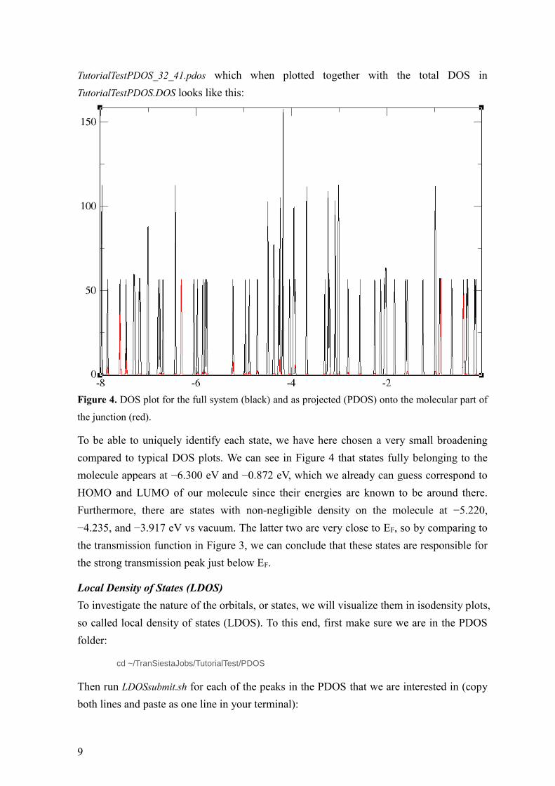
TutorialTestPDOS_32_41.pdos which when plotted together with the total DOS in
TutorialTestPDOS.DOS looks like this:
Figure 4. DOS plot for the full system (black) and as projected (PDOS) onto the molecular part of
the junction (red).
To be able to uniquely identify each state, we have here chosen a very small broadening
compared to typical DOS plots. We can see in Figure 4 that states fully belonging to the
molecule appears at −6.300 eV and −0.872 eV, which we already can guess correspond to
HOMO and LUMO of our molecule since their energies are known to be around there.
Furthermore, there are states with non-negligible density on the molecule at −5.220,
−4.235, and −3.917 eV vs vacuum. The latter two are very close to EF, so by comparing to
the transmission function in Figure 3, we can conclude that these states are responsible for
the strong transmission peak just below EF.
Local Density of States (LDOS)
To investigate the nature of the orbitals, or states, we will visualize them in isodensity plots,
so called local density of states (LDOS). To this end, first make sure we are in the PDOS
folder:
cd ~/TranSiestaJobs/TutorialTest/PDOS
Then run LDOSsubmit.sh for each of the peaks in the PDOS that we are interested in (copy
both lines and paste as one line in your terminal):
10
for E in -6.300 -5.220 -4.235 -3.917 -0.872 -0.398; do echo $E; LDOSsubmit.sh TutorialTestPDOS.fdf $E;
done
These calculations first call on siesta to create .LDOS gridfiles, followed by grid2cube to
create isodensity cube-files. Once entered the queue, they should complete within less than
15 minutes. The resulting cube files can be opened in GaussView or any other compatible
software such as PyMol or Chimera. The cubes are formatted as densities, so a very small
isovalue (~0.0001) must be specified to obtain lobes of reasonable size.
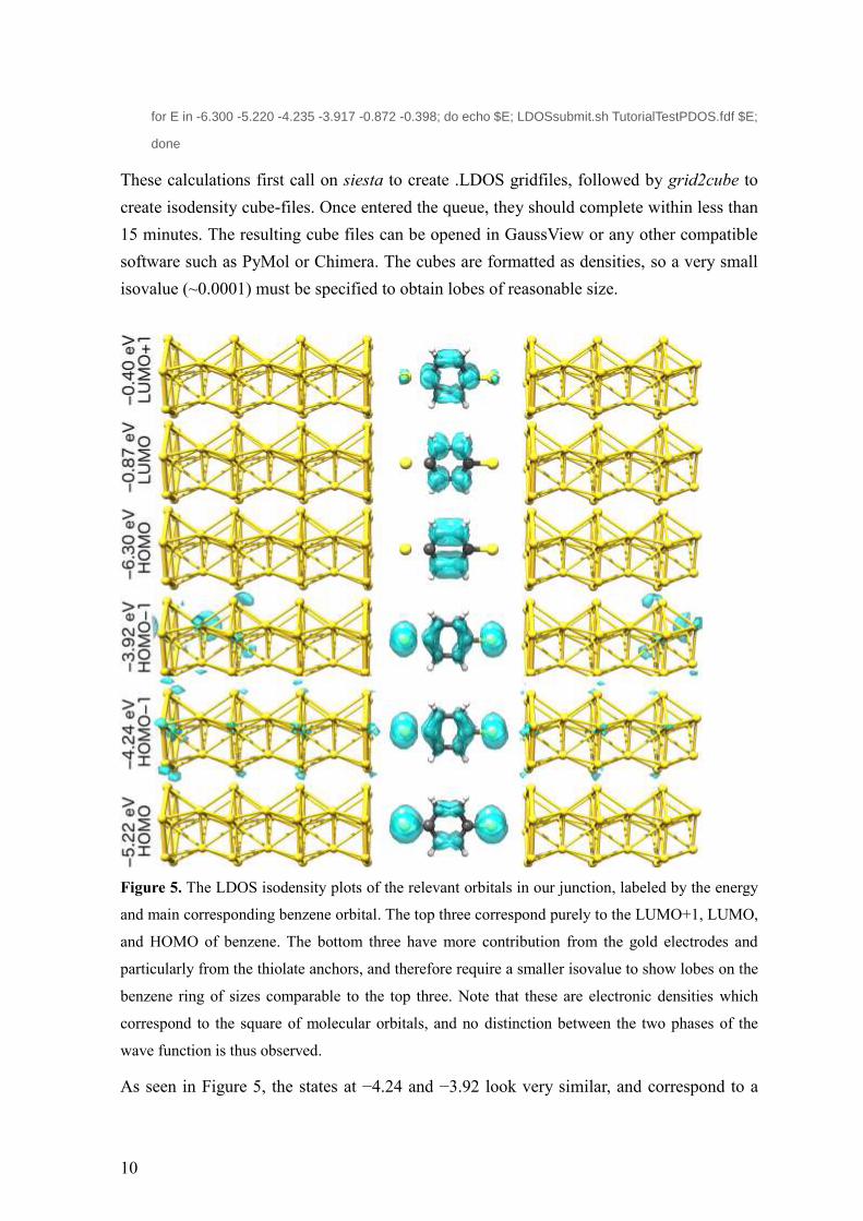
Figure 5. The LDOS isodensity plots of the relevant orbitals in our junction, labeled by the energy
and main corresponding benzene orbital. The top three correspond purely to the LUMO+1, LUMO,
and HOMO of benzene. The bottom three have more contribution from the gold electrodes and
particularly from the thiolate anchors, and therefore require a smaller isovalue to show lobes on the
benzene ring of sizes comparable to the top three. Note that these are electronic densities which
correspond to the square of molecular orbitals, and no distinction between the two phases of the
wave function is thus observed.
As seen in Figure 5, the states at −4.24 and −3.92 look very similar, and correspond to a

11
mix between benzene HOMO−1, sulfur p orbitals, with a small contribution from gold d
orbitals. Due to the interaction with the anchors and the gold electrodes, this orbital has
been split, and is of higher energy than the orbitals corresponding to benzene HOMO. By
comparing to the transmission function in Figure 3, we find out that based on their energy,
these orbitals are responsible for the strong transmission peak just beneath EF.
4. Electrode considerations
The choice of electrode design can affect the transport properties significantly. The
electrode design used above is based on a repeating unit of 20 gold atoms in a hexagonal
close-packing 7–3–7–3 fashion. It shows very good convergence traits but is rather thin,
having a low density of states. The electronic structure of these electrodes are contained in
the file ~/TranSiestaJobs/CommonFiles/AuLeads.TSHS which is used throughout this tutorial.
This file was generated previously in a separate calculation, using a slightly different .fdf
input file than the ones used so far in this tutorial. Some other electrodes designs and
corresponding repeating unit TSHS files can be found on the Grace supercomputer at
/scratch/fas/batista/skh43/TranSiestaJobs/Electrodes. The 1Au65.mol2 and 1Au69.mol2 nanowire
electrode designs are potentially useful, due to ending in a tip rather than a flat surface,
which is a more likely scenario in break-junction experiments, and facilitates the use of
NH2 anchors. Their repeating unit electronic structures are found in Au20.TSHS and
Au18.TSHS respectively.
To create TSHS files for other electrode designs, you must perform calculations of the
corresponding repeating unit. When designing your own electrode, make sure it has its
coordinates aligned along the z-axis, which is also the transport direction, save it as
coords.xyz and run
proper_shift; mv coords_shifted.xyz coords.xyz; change_xyz;
When prompted Please insert the two axis which need to be changed, type
s s
Then run
xyz_to_fdfLead
And choose
1
This will generate an input file coords.fdf for an electrode calculation. The calculation is
submitted to the queue using a standard submission script, containing the line
mpirun –np 12 transiesta < coords.fdf | tee coords.out
which when completed will generate a TSHS file which can be used in subsequent

12
transport calculations, instead of the default one used earlier in this tutorial. Make sure to
copy the newly generated TSHS file to the transport calculation folder before starting the
transport calculation, and edit your transport input file to reflect the filename of your new
TSHS file.
5. Technical details
The bond distances in the above are taken from optimizations of a phenyl-thiolate
bound to a gold electrode. However, the transport properties are quite sensitive to the
binding geometry, so it may be advisable to do some sort of optimization of your
particular system before running the transport calculations. The most rigorous
approach would be to sample a larger part of the conformational space, e.g. by doing
some MD (ab initio or force field) of the junction, and perform transport calculations
on a number of snapshot geometries.
The scripts above apply the DZ basis set for the whole system. Using DZP for the gold
electrodes leads to severe convergence issues, but using DZP for the molecule and DZ
for the electrodes should be fine, probably even preferable.
Pseudopotential files for other elements than those already present, can be found at
http://departments.icmab.es/leem/siesta/Databases/Pseudopotentials/Pseudos_GGA_Abinit
and downloaded to the ~/TranSiestaJobs/CommonFiles folder.
Siesta on Stampede only works with the older intel/13.0.2.14 version as per the fall of
2016, so make sure to load that module rather than the default, newer Intel compiler.
Electrode pairs with an uneven number of gold atoms in total, have proven much more
successful than even numbered ones which tend to yield some rectification even for
completely symmetric molecules.
The PBE functional, as all pure DFT methods, tends to overestimate conjugation and
underestimate the HOMO–LUMO gap. A good way to check for this is to do an
equilibrium, “normal” DFT calculation of your junction (keeping only a small part of
the computationally expensive electrode) with a hybrid functional, such as PBE0 or
B3LYP, and compare the energies of your transmissive orbital(s).