Storing and Analyzing Social Data

University of BaselComputer Science Department

Master Thesis

Author:Nicolas RuflinBreisacherstrasse 264057 Basel+41 76 435 58 67n.ruflin@stud.unibas.ch

Thesis Advisors:Prof. Dr. Helmar Burkhart

Dr. Sven Rizzotti

December 31, 2010

Contents1 Introduction 1

2 From Raw Graph Data to Visualization 42.1 Graph data – Social data . . . . . . . . . . . . . . . . . . . . . . . . . . . . 4

2.1.1 Structure of Social Data . . . . . . . . . . . . . . . . . . . . . . . . 52.1.2 Representation of Social Data . . . . . . . . . . . . . . . . . . . . . 62.1.3 Data providers . . . . . . . . . . . . . . . . . . . . . . . . . . . . . 7

2.2 Social data graph analysis . . . . . . . . . . . . . . . . . . . . . . . . . . . . 82.2.1 Graph Theory – Centrality . . . . . . . . . . . . . . . . . . . . . . . 92.2.2 Degree Centrality . . . . . . . . . . . . . . . . . . . . . . . . . . . . 102.2.3 PageRank . . . . . . . . . . . . . . . . . . . . . . . . . . . . . . . . 112.2.4 Data processing . . . . . . . . . . . . . . . . . . . . . . . . . . . . . 12

2.3 Storage systems . . . . . . . . . . . . . . . . . . . . . . . . . . . . . . . . . 152.3.1 CAP, Dynamo and BigTable . . . . . . . . . . . . . . . . . . . . . . 172.3.2 Relational database management system (RDBMS) . . . . . . . . . . 192.3.3 Key-value stores . . . . . . . . . . . . . . . . . . . . . . . . . . . . 192.3.4 Column stores . . . . . . . . . . . . . . . . . . . . . . . . . . . . . 202.3.5 Document stores . . . . . . . . . . . . . . . . . . . . . . . . . . . . 212.3.6 Graph databases . . . . . . . . . . . . . . . . . . . . . . . . . . . . 21

2.4 Data visualization . . . . . . . . . . . . . . . . . . . . . . . . . . . . . . . . 22

3 Data, Methods & Implementation 243.1 useKit Data . . . . . . . . . . . . . . . . . . . . . . . . . . . . . . . . . . . 243.2 Social graph analysis . . . . . . . . . . . . . . . . . . . . . . . . . . . . . . 28

3.2.1 Degree centrality . . . . . . . . . . . . . . . . . . . . . . . . . . . . 283.2.2 PageRank . . . . . . . . . . . . . . . . . . . . . . . . . . . . . . . . 29

3.3 Storage systems and their data models . . . . . . . . . . . . . . . . . . . . . 303.3.1 MySQL . . . . . . . . . . . . . . . . . . . . . . . . . . . . . . . . . 313.3.2 Redis . . . . . . . . . . . . . . . . . . . . . . . . . . . . . . . . . . 333.3.3 Riak . . . . . . . . . . . . . . . . . . . . . . . . . . . . . . . . . . . 353.3.4 MongoDB . . . . . . . . . . . . . . . . . . . . . . . . . . . . . . . 373.3.5 CouchDB . . . . . . . . . . . . . . . . . . . . . . . . . . . . . . . . 393.3.6 HBase . . . . . . . . . . . . . . . . . . . . . . . . . . . . . . . . . . 413.3.7 Cassandra . . . . . . . . . . . . . . . . . . . . . . . . . . . . . . . . 443.3.8 Neo4j . . . . . . . . . . . . . . . . . . . . . . . . . . . . . . . . . . 45

3.4 Visualization . . . . . . . . . . . . . . . . . . . . . . . . . . . . . . . . . . 463.5 Experiment setup . . . . . . . . . . . . . . . . . . . . . . . . . . . . . . . . 48

4 Analysis and Results 494.1 Data structure . . . . . . . . . . . . . . . . . . . . . . . . . . . . . . . . . . 49

4.1.1 Social data . . . . . . . . . . . . . . . . . . . . . . . . . . . . . . . 494.1.2 useKit Data . . . . . . . . . . . . . . . . . . . . . . . . . . . . . . . 50

4.2 Network analysis . . . . . . . . . . . . . . . . . . . . . . . . . . . . . . . . 514.2.1 Degree centrality . . . . . . . . . . . . . . . . . . . . . . . . . . . . 514.2.2 PageRank . . . . . . . . . . . . . . . . . . . . . . . . . . . . . . . . 53

4.3 Storage systems . . . . . . . . . . . . . . . . . . . . . . . . . . . . . . . . . 544.3.1 Data model . . . . . . . . . . . . . . . . . . . . . . . . . . . . . . . 554.3.2 Social Data . . . . . . . . . . . . . . . . . . . . . . . . . . . . . . . 574.3.3 Queries & Data Processing . . . . . . . . . . . . . . . . . . . . . . . 584.3.4 Degree centrality . . . . . . . . . . . . . . . . . . . . . . . . . . . . 594.3.5 PageRank . . . . . . . . . . . . . . . . . . . . . . . . . . . . . . . . 604.3.6 Scalability . . . . . . . . . . . . . . . . . . . . . . . . . . . . . . . 614.3.7 General survey . . . . . . . . . . . . . . . . . . . . . . . . . . . . . 63

4.4 Visualization . . . . . . . . . . . . . . . . . . . . . . . . . . . . . . . . . . 64

5 Discussion & Future Work 675.1 Data . . . . . . . . . . . . . . . . . . . . . . . . . . . . . . . . . . . . . . . 675.2 Storage systems . . . . . . . . . . . . . . . . . . . . . . . . . . . . . . . . . 675.3 Processing / Analyzing . . . . . . . . . . . . . . . . . . . . . . . . . . . . . 705.4 Visualization of Graph Data . . . . . . . . . . . . . . . . . . . . . . . . . . 72

6 Conclusion 74

AbstractSocial platforms such as Facebook and Twitter have been growing exponentiallyin the last few years. As a result of this growth, the amount of social data increasedenormously. The need for storing and analyzing social data became crucial. Newstorage solutions – also called NoSQL – were therefore created to fulfill this need.This thesis will analyze the structure of social data and give an overview of cur-rently used storage systems and their respective advantages and disadvantages fordifferently structured social data. Thus, the main goal of this thesis is to find outthe structure of social data and to identify which types of storage systems are suit-able for storing and processing social data. Based on concrete implementations ofthe different storage systems it is analyzed which solutions fit which type of dataand how the data can be processed and analyzed in the respective system. A fo-cus lies on simple analyzing methods such as the degree centrality and simplifiedPageRank calculations.

Target reader group: Designers and developers of social networks.

1 IntroductionToday’s omnipresence of social data is to some extent associated with the development ofthe Internet, which is the result of the the Advanced Research Projects Agency Network(ARPANET)[1]. The ARPANET was a computer network which came to be the foundation ofthe global internet as we know it today. It was created in the United States and launched witha message – or the first form of social data in the internet – that was sent via the ARPANETon 29 October 1969.

Although social data does not exclusively come from the Internet – also telephones, sensorsor mobile devices provide social data – the predominant part of social data is in fact internetbased. It started with the exchange of information via e-mail. Soon, e-mails could be sent toseveral people at once. The next steps were mailing lists, fora and blogs with commentingfunctions. Later, social networks followed. It is then that the amount of data became a massphenomenon. With social platforms such as Facebook or Twitter, the upswing of social datawas as strong that today, it has become a standard medium. As a result of the exponentialincrease in social data, the need for storing and analyzing it has become a challenge that hasyet to be solved.

The goal of this thesis is to analyze the structure of social data and to give an overviewof already existing algorithms to analyze and process social data, implemented on differentstorage systems and based on a specific data set. In addition, the data set will be visualized.As opposed to more research-oriented papers, this thesis combines four different researchareas – structure, storage, processing and visualization of social data, as is portrayed in figure1 – and implements them in a real-world example. Although each of these four areas hasbeen researched extensively and relevant findings have been made, the findings of each areahave rarely been brought together to see the overall picture. Thus, researchers in one areaonly seldomly have access to discoveries that were made in another area. This is what makes

1

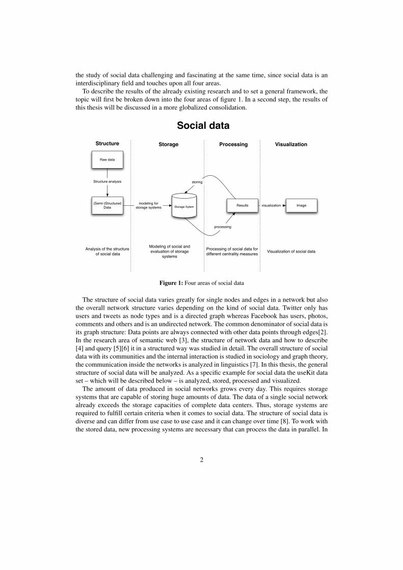
the study of social data challenging and fascinating at the same time, since social data is aninterdisciplinary field and touches upon all four areas.

To describe the results of the already existing research and to set a general framework, thetopic will first be broken down into the four areas of figure 1. In a second step, the results ofthis thesis will be discussed in a more globalized consolidation.

Analysis of the structure of social data

Modeling of social and evaluation of storage

systems

Processing of social data for different centrality measures Visualization of social data

Social dataStructure Storage Processing Visualization

Raw data

(Semi-)Structured Data Storage Sytem

Structure analysis

modeling for storage systems Results Image

processing

storing

visualization

Figure 1: Four areas of social data

The structure of social data varies greatly for single nodes and edges in a network but alsothe overall network structure varies depending on the kind of social data. Twitter only hasusers and tweets as node types and is a directed graph whereas Facebook has users, photos,comments and others and is an undirected network. The common denominator of social data isits graph structure: Data points are always connected with other data points through edges[2].In the research area of semantic web [3], the structure of network data and how to describe[4] and query [5][6] it in a structured way was studied in detail. The overall structure of socialdata with its communities and the internal interaction is studied in sociology and graph theory,the communication inside the networks is analyzed in linguistics [7]. In this thesis, the generalstructure of social data will be analyzed. As a specific example for social data the useKit dataset – which will be described below – is analyzed, stored, processed and visualized.

The amount of data produced in social networks grows every day. This requires storagesystems that are capable of storing huge amounts of data. The data of a single social networkalready exceeds the storage capacities of complete data centers. Thus, storage systems arerequired to fulfill certain criteria when it comes to social data. The structure of social data isdiverse and can differ from use case to use case and it can change over time [8]. To work withthe stored data, new processing systems are necessary that can process the data in parallel. In

2

this thesis, five different storage system types are analyzed by applying them to the useKit dataset in order to evaluate how suitable they are for storing social data. The five storage systemtypes are: key-value stores, column stores, document stores, graph databases and RDBMS.

Processing the stored data is crucial in order to extract relevant data out of the stored data[9]. There are different methods of how data sets can be queried or processed. Parts of theresearch community use implementations for processing social data which are based on su-percomputers such as the Cray [10] [11]. Others focus on providing processing methods thatcan scale up to thousands of commodity machines to provide the same processing power [12].The commodity hardware approach is also more adequate for social network companies suchas Facebook, Twitter and LinkedIn that have to process large amounts of data. One of thede facto standards for processing large amounts of data on commodity hardware is currentlythe MapReduce model [13], which is also extensively used in this thesis. However, as thedata changes rapidly and constantly, there is a need for improved and more efficient methods.In this thesis, the emphasis lies on processing the nodes for centrality measures. Centralitymeasures of a node in a network can describe the relevance, influence or power of a node ina network. Two centrality measures – degree centrality and PageRank – are implemented inevery storage system with the specific capabilities of every single system to process the dataset.

Visualizing information was already used a long time ago by the Greeks and Romans tocommunicate and to show concrete ideas. One of the main goals of information visualizationis the representation of the data in a way that makes it visually appealing and understandableby the consumer [14]. Initially, data visualization in computer science focused on the researcharea of computer graphics. From there, the visualization of information through computers andalgorithms has made its ways in almost every other research area. Nevertheless, visualizationis still in its infancy. Basic algorithms based on physical laws are used to create the visualrepresentation [15]. But often, human interaction is still necessary, because the human feelingof how a graph representation is comfortable is not only based on mathematical rules [16].With the growth of the internet and social data, visualization is used to visualize the relationsor the structure of these networks, but also in other ways such as to show how the swine fluespreads over the world, which was done in 2009 by Google. Data visualization often makesdata better understandable and can reveal unknown details such as communities or clusters ina network, but also describe the overall data structure. In this thesis, different methods wereevaluated to visualize graphs with more than 100’000 nodes and edges. The useKit data setwas visualized in order to better understand the overall structure.

Every section of this thesis is split up into four parts as shown in figure 1: data structure,data processing, data storage and data visualization. In the first part of the thesis, the structureof social data 2.1, especially the structure of the useKit data 3.1 is analyzed. The second partevaluates the different types of storage systems 2.3 in detail based on eight different storagesystems 3.3 – MySQL, Redis, Riak, MongoDB, CouchDB, HBase, Cassandra, Neo4j – inorder to show the advantages of every single system. The useKit data is modeled for everysystem and stored inside the system. In the next section, processing methods to calculatedegree centrality and PageRank 2.2 for the useKit data are shown for every system 3.3. Tobetter understand the complete structure of the useKit data, the data is visualized in the end3.4.

3

2 From Raw Graph Data to VisualizationGraph data is an elementary part of most data sets in research, business, social networks andothers. Current computers are good in running sequential algorithms and also store data se-quentially. To represent graphs in computer memory often adjacency matrices are used whichis efficient as long as the complete graph data set fits into memory. Storing graphs that do notfit onto one machine in an efficient way is still an open problem. Until a few years ago therewere only a few graph data sets that had millions of nodes. With the growth of social networksmore and more huge graph data sets exist which have to be stored and processed. To store,process and analyze social data it is crucial to understand the structure of social data and howit can be represented.

First, the structure and representations of graph data and social data will be described indetail. In a second step, the different algorithms that are used in this thesis to process andanalyze the social data will be described. This will be followed by a part on existing storageand processing systems. Then visualization algorithms and methods are described in detail.

2.1 Graph data – Social dataLarge quantities of digital data are created every day by people and computers. As soon as thedata consists of data points that are related or there are relations within the data, the respectivedata can be represented as a graph or network [17]. Examples for such data sets are data setsof chemical systems, biological systems, neural networks, DNA, the world wide web or socialdata created by social platforms. Social data can be represented as a graph because of therelations between its nodes which often means users are connected to other users.

Social data is produced by users that interact with other users, but also machines can createsocial data. There are coffee machines that tweet every time someone gets a coffee or mobilephones that automatically send the current location of a user to one or several social platforms.Also different social platforms can be connected to each other to automatically update a per-son’s status on other platforms. Adding a twitter account to your own Facebook profile meansthat every time a message is posted on Facebook, it is automatically tweeted. Thus, a singleinput produces several data entries.

The term social graph describes the data in social platforms including its relationships toother nodes. The term is also used by Facebook to describe its own data set. There does notappear to be any formal definition of a social graph. In general, every social network hasits own social graph but by having more and more social platforms connected to each otherthese social graphs also start to overlap. Because there are no standards for social graphs,one main concern is the portability of social data between platforms. Brad Fitzpatrick hasposted his thoughts on the social graph in the blog post “Thoughts on the Social Graph” [18]and mentions some interesting points about the owner ship of the social graph and if thereshould be a standard way to access it. He discusses how the storage of a social graph, whichmeans storing social data, could be decentralized and perhaps also on the client side insteadof trusting in one large company that stores and manages all data.

Definition of social data There are different approaches to define social data. In theresearch area of linguistics, social data is better known under the term computer-mediated

4

communication (CMC) and can be defined as “predominantly text-based human-human inter-action mediated by networked computers or mobile telephony” [7]. Because I did not find anexact technical definition of social data, in this thesis social data is defined even broader as datathat is produced by individuals or indirectly by machines through interaction by individuals(coffee machine) that is published on a data store (social platform, forum etc.) accessible byother individuals and that allows interaction (comments, response, like etc.). Every data pointhas at least one connection to another data point. Examples of social data are forum entries,comments on social platforms or tweets, but also data like GPS locations that are sent frommobile devices to social platforms.

One of the simplest forms of social data produced in the internet is probably email. Emailsare sent daily from one user to several users to communicate and to exchange data. This startedin 1970 with the invention of the internet. The next step in evolution were mailing lists, forums,wikis (Wikipedia), e-learning systems and other types of social software. The produced datawas limited to a relatively small number of participants. Around 2006 the so-called Web 2.0started and platforms like Facebook, Orkut and others started to grow rapidly. The numberof users that exchanged social data grew exponentially and new requirements to process thismassive amount of data appeared. When data was no longer simply exchanged between 5 or10 users, data started to be exchanged between hundreds or thousands of nodes and couldbe access by a lot more because most of the data is public available. Currently, Facebook hasmore than 500 million users [19]. This means that Facebook is a network or a graph with morethan 500 million vertices and billions of edges.

As Stanley Milgram found out back in 1960 with his famous and widely accepted small-world experiments [20], the average distance between two people is 5.9. Therefore, most peo-ple are on average connected to everyone else over six nodes. It is therefore likely that thesesocial networks have a similar value of connectability – possibly even lower, since Facebookhas a tendency to connect more people than real life, since people can be contacted easily andeffortlessly.

2.1.1 Structure of Social Data

There are no predefined data models for the structure of social data. Social data appears in abroad variety of forms and its structure differs from use case to use case. Also, the structuremight vary within a use case, and it can evolve over time. Let us take location data as anexample. Nowadays, lots of mobile devices included GPS but have different capabilities. Someonly send data +-100m accurate, others include also sea height and more precise details. Thestructure of the data depends on the system that sends the data and on its capabilities. Eventhough the exact structure of the data that is sent is not known in advance, storage systemshave to be capable to store the data. One option is to filter all incoming data and discard allinformation that is not supported by all systems, but this means loosing relevant data. An otherapproach is to store all data even though the data structure can be different for every packagewhich poses special requirements on the storage systems.

The structure of social network data is different from web link data. Web link data consistsof webpages and the connecting links. It can be represented as a directed graph because everylink goes only in one direction. There is a distinct difference between social data and weblink data as Bahmani describes: “In social networks, there is no equivalent of a web host, and

5

more generally it is not easy to find a corresponding block structure (even if such a structureactually exists)” [8]. This difference has a direct effect on the storing and retrieving of socialdata, because similar data cannot be stored together on one machine. This again has a directaffect on data accessing and processing, because calculations are even more distributed and itis hard to minimize communication. Typical for the social data structure is the N to N relationsthat exist for most nodes, which means every node connects to several nodes, and several othernodes are connected to this node.

Social data can be represented as a graph. In the example of Facebook, every node is a userand the connections between the users are edges. Research has shown that social networks inthe real wold and also computer-based social networks such as Facebook are fat tailed net-works. Thus, they differ from random graphs [17]. This means that at the tails of the network,there are highly connected networks in comparison to the connectivity to the rest of the net-work. We see the same phenomenon in the real world: it is highly probable that people whoknow each other also know each other’s friends – they are highly connected – and they knowconsiderably less people in the rest of the world – less connectivity in the network overall.

In social networks, there are often some highly connected nodes. In social networks suchas Facebook or Twitter, these are often famous people. Based on the power law, these nodesare exponentially more popular than others nodes. In June 2009, the average user on Twitterhad around 126 followers[21]. But there are some users with more than two million followers[22], and the number increases fast.

2.1.2 Representation of Social Data

For every data set there are different methods to represent the data. The different represen-tations can be used for different tasks and every representation has its advantages and disad-vantages. It is crucial to find the right data representation for a specific task. In the following,different methods of representing social data are described.

One of the simplest ways of representing a graph is with dots (vertices) and lines (edges)[2].With simple dots and lines, every graph can be represented and visualized. Thus, also socialdata can be represented with dots and lines. In social networks, every user is a vertex andevery connection to another user is an edge. However, additional parameters for vertices andedges are often desired to also represent specific values of the vertices and describe the edgesin more detail. This can be done with a so-called property graph [23].

The DOT Language [24] defines a simple grammar to represent graphs as pure text filesthat are readable by people and computers. Every line in the file consists of two vertices andthe edge in between. The DOT Language allows to set properties for edges and vertices andto define subgraph structure. The created files are used by Graphviz to process and visualizegraphs.

Lots of research has been done in the area of semantic web – also called the web of data [25].The goal of the semantic web is to give computer understandable meaning to nodes and theconnections in between various types of nodes. It is possible to assign a semantic meaning tomost relations in social networks. This makes it possible to use social data as semantic data andprocess it by computers. One common way to represent relations in graph data is the ResourceDescription Framework (RDF) [4], which is based on XML from the semantic web movement

6

created by W3C1. RDF is a standard model that interchanges semantic data on the web. EveryRDF triple consists of subject, predicate and object. To map these properties to a graph, subjectand object are represented as vertices, predicate as an edge. This makes it possible to representevery type of graph. Converting social data into a RDF representation makes social networkssearchable by SPARQL. A computer is therefore able to query the data based on constraints,even though the computer does not understand the data. The Friends of a Friend (FOAF)2

project is another approach that is more focused on representing social data in a standardizedway and that has as its goal to make sharing and exchanging information about the connectionsand activities of people easier. FOAF is based on RDF with predefined properties that canbe used to name the edges. Another approach in this area is the Web Ontology Language(OWL) [26]. The overall goal of these representations of social data is to make it readable andsearchable by computers.

Another representation of graph data often used in high performance computing in combi-nation with matrix calculations is the representation as an adjacency matrix. These matricesare often sparse matrices, which makes it possible to store data in a compressed form as thecompressed sparse row (CSR) format and others[27][28]. Much research has been conductedon the processing and storing of sparse matrices [29][30]. Matrices or multidimensional arraysare a forms of data representation that fit computer memory and processor structures well.

Another approach to represent graph data or social data is the JavaScript Object Notation(JSON)[31]. JSON can represent complex structures in a compact way and is also readableby people. JSON has a loose type system and supports objects and arrays. This allows torepresent graph data with subarrays and can be used to represent single nodes and edges withtheir properties or small networks with an initial node. Because of its compact form and itssupport in most programming languages, JSON has been becoming one of the standards ininterchanging data between different services and often also replaces XML. The JSON formathas found adoption in storage systems to store data and query data as in Riak or MongoDB.

For people, the representation of a graph that is most easily understandable is the represen-tation as an image. To create such an image, the graph has to be processed first. Visualizinggraph data for people is not only based on pure mathematical and physical, rules but also onthe sensation of the viewer [14]. This makes it a complex subject that is researched thoroughly.In contrast, image representation is difficult to understand for computers. Thus, other formatsthat were mentioned above are used for the internal representation and storage.

2.1.3 Data providers

To store, process and analyze social data sets real world examples with a adequate size arenecessary. There are different open data sets mostly created by research or the open sourcecommunity. Most of these public data sets are web link data sets or similar, real world socialdata sets are rare.

Some of the first open data repositories where data was analyzed in depth were citationnetworks [32] and the Usenet [33]. There are also open data repositories such as DBPedia[34], Geonames and others which have already been analyzed in research [35] [36]. The Many

1The World Wide Web Consortium (W3C): http://www.w3.org/2Friends of a Friend project: http://www.foaf-project.org/

7

Eyes project from IBM 3 is an open project that allows daily users and researchers to uploadtheir own data and to visualize it with the existing tools. The platform is also used by theUniversity of Victoria, Canada, for research. A web link data set that was created for researchis the ClueWeb094 collection [37]. The goal of this collection was to support research oninformation retrieval and related human language technologies. The data set consists of morethan 1 billion pages in 10 different languages and has a size of 5 TB. It was collected inJanuary and February 2009 and was used in different research projects such as for examplethe TREC 2009 Web Track[38].

For the analysis in this thesis a data set from a social network is needed. Even if a hugeamount of social data is produced every day, the access to social data is protected. Every socialnetwork secures its own data to protect the privacy of its users and to make it impossible to giveinsight to competitors. Most social networks have an API as Facebook with the Open Graphprotocol 5 or Google with its social graph API 6 and the Google GData Protocol 7 which allowsto access parts of the data. There are two main problems when using such a large amount ofsocial data for research. To access hidden user data, every user has to confirm the access first.Moreover, it is often not possible to store data that is retrieved from social networks locallyfor more than 24 hours, which prevents people from retrieving a large amount of data forprocessing purposes. Some research institutes are working together with social network dataproviders, which allows them to access the data directly.

2.2 Social data graph analysisSocial data graph analysis describes the process of analyzing the data of which a social graphconsists of. One of the main goals of analyzing a social graph is to better understand thestructure of the graph and find important nodes inside the graph. To find important nodesdifferent algorithms can be used as centrality measures like degree centrality or PageRank. Tobetter understand the complete structure of the graph community identification or visualizingthe graph can help. Implementing these centrality measures on different storage systems toanalyze the stored graph data is a central part of this thesis.

The main challenge with the analysis of social data is the amount of data that already existsand the data that is constantly produced. The amount of data has exceeded the storage capaci-ties of one single machine a long time ago. Thus, the data needs to be stored in larger clusters.The graphs that have to be analyzed have millions to billions of nodes and edges, which alsomakes it impossible to process them on a single machine. To analyze only a subset of the exist-ing graph data, key problems are finding communities which are dense collections of vertices,splitting up graphs with coarsening and refinement or local clustering. Different approaches tofind communities with parallel computers on peta scale graphs have been described by Bader[39]. For research, there are massively multithreaded and shared memory systems such as theCray computer that are used for large graph processing [10] [11] [40]. Such systems are rareand expensive and also have scalability limits.

3IBM ManyEyes Project page: http://manyeyes.alphaworks.ibm.com/manyeyes/4ClubWeb09 data set: http://boston.lti.cs.cmu.edu/Data/clueweb09/5Facebook API to include Facebook content in other webpages: http://opengraphprotocol.org/6Google API to make public connections useful: http://code.google.com/apis/socialgraph/7GData APi: http://code.google.com/apis/gdata/

8

Distributed solutions for storing, processing and analyzing social graph data are neededbecause many graphs of interest cannot be analyzed on a single machine because of its span-ning on millions of vertices and billions of edges [41]. Based on this, lots of companies andresearchers moved to distributed solutions to analyze this huge amount of data. Similar prob-lems are tackled in the research area of data warehousing . Companies such as Facebook orGoogle which have large graph data sets store, process and analyze their data on commod-ity hardware. The most common processing model used is MapReduce [13]. Analyzing dataon distributed systems is not a simple task since related nodes are distributed over differentmachine. This again leads to a lot of communication. The first approach that was tried wasstoring related nodes on the same machine to minimize queries over several machines. But asFacebook stated the structure of social data is dynamic and not predictable which leads to theconstant restructuring of the system. The conclusion was to randomly distribute the nodes onthe machines and not do any preprocessing.

Until october 2010 in most areas there was a clear distinction between instantaneous dataquerying and the delayed data processing. Data processing on large data sets was done basedon MapReduce and retrieving the result could take from several minutes up to days. Whenevernew data was added to the data set, the complete data set had to be reprocessed which istypical for the MapReduce paradigm. This was changed by Google in October 2010 throughthe presentation of their live search index system Caffeine[42] which is based on the scalableinfrastructure Pregel [12]. Pregel allows to dynamically add and update nodes in the systemand the added or modified nodes can be processed without having to reprocess the whole dataset.

2.2.1 Graph Theory – Centrality

Every graph consists of edges and vertices. In this thesis, a graph is defined as G = (V, E)where vertices V stand for the nodes in the graph, and edges E for the links or connectionsbetween the nodes. This is the standard definition that is mostly used for social data and othergraph data. Edges in a graph can be undirected or directed, depending on the graph.

One of the most common tasks for graphs is to find the shortest path between two nodes,which is also called the geodesic distance between two nodes. There are different algorithmsto solve the problem of the shortest path. The Dijkstra algorithm solves the single-sourceshortest path problem. It has a complexity of O(V 2) for connected graphs, but can be opti-mized to O(|E| + |V |log|V |) for sparse graphs and a Fibonacci heap implementation. TheBellman-Ford algorithm is similar to the Dijkstra algorithm, but is also able to solve graphswith negative edges and runs in O(|V ||E|).

To calculate all shortest paths in a graph the Floyd-Warshall algorithm can be used. TheFloyd-Warshall algorithm calculates all shortest paths with a complexity of O(n3). Becauseof its exponential complexity it cannot be used for large graphs. Most graphs in the areaof social data that are analyzed are sparse graphs. The Johnson algorithm is similar to theFloyd-Warshall but it is more efficient on sparse matrices. It uses the Bellman-Ford algorithmto eliminate negative edges and the Dijkstra algorithm to calculate all shortest paths. Is theDijkstra algorithm implemented as a Fibonacci heap, all shortest paths can be calculated inO(V 2logV + V E).

9

Because shortest path algorithms are crucial for graph processing such as centrality calcu-lations, many researchers worked on optimizing these algorithms. Brandes has shown that be-tweenness centrality [43] on unweighted graphs can be calculated with O(EV ) and O(EV +E2log(E) for weighted graphs [44]. This made it possible to extend centrality calculations tolarger graphs.

There are various centrality algorithms for a vertex in a graph. The centrality of a person ina social network describes how relevant the person is for the network and, as a consequence,how much power a person has. However, as Hanneman [43] describes, influence does notnecessarily mean power.

In the following, degree centrality and PageRank are described in detail. The implementa-tions of these two will be made for data processing. Other centrality measures such as close-ness, betweenness and stress centrality or the more complex Katz centrality, which have beendescribed in detail by Hannemann and Riddle[43] have been extensively researched in recentyears. Also parallel algorithms were developed to evaluate centrality indices for massive datasets in parallel [11] [45]. Calculating shortest paths between vertices is crucial for most ofthese algorithms.

Another centrality approach that was proposed by Lempel and Moran is the StochasticApproach for Link-Structure Analysis (SALSA) [46]. SALSA is based upon Markov chainsand is a stochastic approach for link structure analysis. The authors distinguish between so-called hubs and authorities. The goal of the SALSA-algorithm is to find good authorities,which can be compared to nodes that have a high centrality degree.

2.2.2 Degree Centrality

There are two different types of degree centrality, one defined by Freeman [47] and a newerversion defined by Bonacich [48]. The latter also takes into account to which nodes a certainnode is connected to. In this thesis, it is assumed that a node, which is connected to lots ofother nodes with high degree, probably also has a more central position in the network than anode that is connected to lots of nodes without connections. This is an idea that can also befound in the PageRank algorithm.

The Freeman approach is defined as the sum of all edges connected to a node and differ-entiates between in and out degree for directed graphs. Every edge can have an edge weightwhich is the value in the sum for the connected vertex. In unweighted and undirected graphs,the Freeman degree centrality is simply the count of all edges that are connected to a node. Fornormalization reasons, this sum is divided by the total number of vertices in the network minusone. The complexity is O(1), which makes it simple and efficient to calculate. The equation isshown in in figure 1, where deg(v) is the count of edges that vertex v has. This is divided bythe total number of edges n in the network minus one. The result is the degree centrality forvertex v.

CD(v) = deg(v)n− 1 (1)

In figure 2 a small network graph with 15 nodes and directed but unweighted edges is shown.In this example, node 1 would have an in-degree of 2, node 2 and in-degree of 5 and and out-degree of 1 because it has 5 incoming edges from node 3,4,5,6 and 15 and one outgoing edge

10

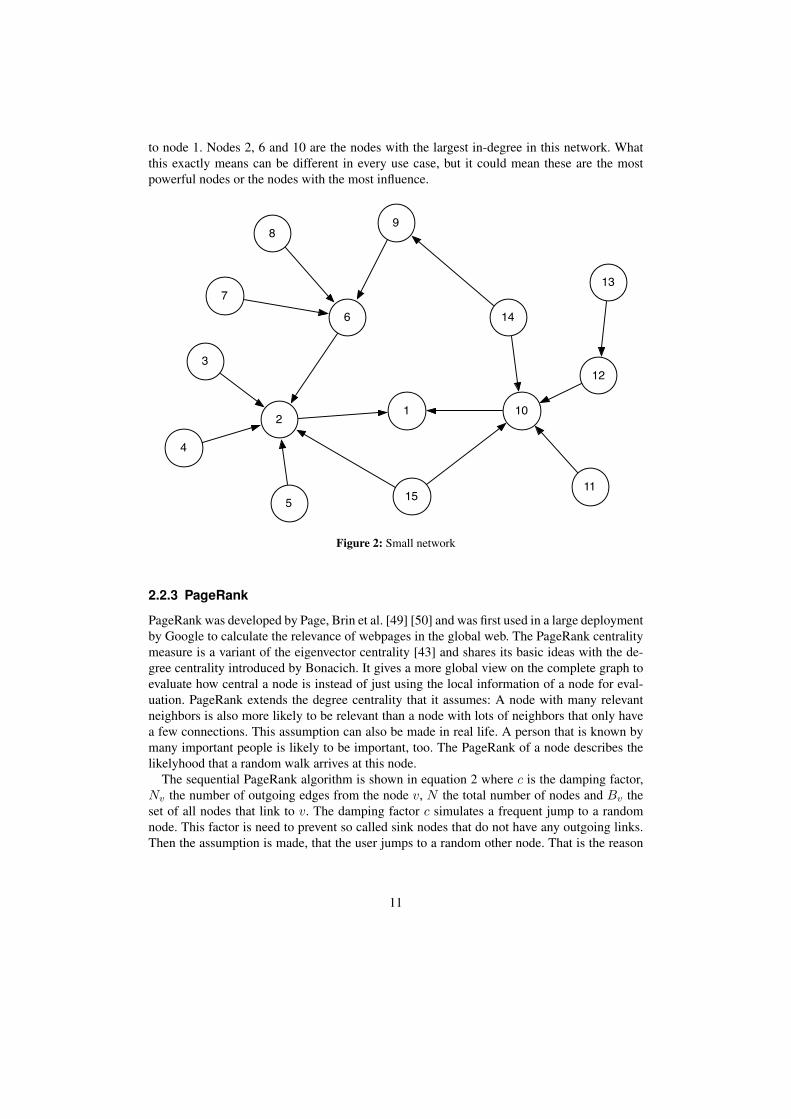
to node 1. Nodes 2, 6 and 10 are the nodes with the largest in-degree in this network. Whatthis exactly means can be different in every use case, but it could mean these are the mostpowerful nodes or the nodes with the most influence.

6

1

5

4

98

2

3

10

12

11

14

137

15

Figure 2: Small network

2.2.3 PageRank

PageRank was developed by Page, Brin et al. [49] [50] and was first used in a large deploymentby Google to calculate the relevance of webpages in the global web. The PageRank centralitymeasure is a variant of the eigenvector centrality [43] and shares its basic ideas with the de-gree centrality introduced by Bonacich. It gives a more global view on the complete graph toevaluate how central a node is instead of just using the local information of a node for eval-uation. PageRank extends the degree centrality that it assumes: A node with many relevantneighbors is also more likely to be relevant than a node with lots of neighbors that only havea few connections. This assumption can also be made in real life. A person that is known bymany important people is likely to be important, too. The PageRank of a node describes thelikelyhood that a random walk arrives at this node.

The sequential PageRank algorithm is shown in equation 2 where c is the damping factor,Nv the number of outgoing edges from the node v, N the total number of nodes and Bv theset of all nodes that link to v. The damping factor c simulates a frequent jump to a randomnode. This factor is need to prevent so called sink nodes that do not have any outgoing links.Then the assumption is made, that the user jumps to a random other node. That is the reason

11

that parts of the PageRank value are equally distributed to every node by the right part of theequation. The smaller the damping factor, the more often random jumps happen. Good valuesfor c seem to be between 0.7 and 0.8. The calculation of the PageRank is an iterative process,which means that the previous results of an iteration are always used for the next iteration.Consequently, intermediate results have to be stored. If the damping factor c is set to 1, thePageRank algorithm equates to the eigenvector centrality. The PageRank algorithm convergesto a static state.

P ′(u) = c∑

v∈Bv

P ′(v)Nv

+ 1− c

N(2)

In figure 2 as described before with the degree centrality, a small network graph is shown.Node 1 in the network had an in-degree of 2, which made it a less central node than 2, 6 or10. With the PageRank the node 1 gets more important because the importance of neighbornodes is also taken into account. Node number 1 has two incoming edges from the two centralnodes 2 and 10. This makes node number 1 more central then node 6 which has three incomingedges from node 7, 8 and 9. But these three nodes do not have any incoming edges from otherimportant nodes or do not have incoming edges at all.

The personalized PageRank algorithm is a modification of the existing algorithm. Insteadof jumping to a random node with a given probability, the jump is always done to the ini-tial node. This creates PageRank values that are more personalized on the focus of the givenuser. Nodes that are relevant for a user do not need to have the same relevance for others.This makes recommendations and personalized search results possible. Experiments have beendone by Twitter in combination with FlockDB8 to implement a fast and incremental personal-ized PageRank[8].

2.2.4 Data processing

Data processing plays a key role in all areas where a large amount of digital data is producedand the goal is to understand the data. A quote form Todd Hoff [9] describes that it is notenough to simply process data in order to make sense of it, but also human analysis is neces-sary:

“There’s just a lot more intelligence required to make sense out of a piece ofdata than we realize. The reaction taken to this data once it becomes informationrequires analysis; human analysis.”

To process data, a data storage system is needed that allows to load or query the data in anefficient way and is also capable of storing the results that come from the processing system.

All data processed in this thesis has a graph structure. The processing and analyzing ofgraph structures was already analyzed in detail in the semantic web movement where thegraph structure is stored as RDF. Much research has been conducted to find out how RDF datacan be stored and queried in an efficient way [51][52][53]. The default query language forthese kinds of data sets is SPARQL [5] or one of its enhanced versions [6]. Typical queries are

8Distributed and fault tolerant graph db with MySQL as storage engine: http://github.com/twitter/flockdb

12

graph traversal queries and finding nodes with predefined edges in between. An example querycould be to find all students that have grades over 5, listen to classical music and like to readbooks. For this, the focus is on graph traversal. In this thesis, the focus is more on processingcomplete data sets to identify the structure of the whole network and on calculating centralityindices of every single node.

Efficient processing of large graph data is a challenge in research as well as for many com-panies. The main challenge is that the complete graph cannot be held in the memory of onemachine [41]. In research, one of the approaches is to use massive shared memory systemssuch as the Cray that can hold the complete graph in memory. Because of the rare availabilityof such machines, most companies process their data on lots of connected commodity hard-ware machines. The main challenge is the communication overhead that is produced duringprocessing the graph. Because of the connections between the data nodes that are distributedon different machines communication is necessary as soon as the calculation for one nodeincludes values of other nodes.

New methods to process data at a large scale more efficiently have already appeared, as forexample the Pregel [12] system that is used by Google. Pregel is a system for graph processingat large scale. Google uses it interally to keep its search index up-to-date and to deliver almostlive search results. Pregel is based on the Google File System (GFS) and supports transactionsand functions similar to triggers. In contrast to most systems which are optimized for instan-taneous return, the goal of Pregel is not to respond as quickly as possible, but to be consistent.Transactions can take up to several minutes because of locks that are not freed. Before Pregel,the data was processed with MapReduce. Large amounts of data had to be reprocessed everytime new nodes and edges were discovered. The new system only updates the affected nodeswhich makes it much more scalable. To analyze and query the given data, Google developedDremel [54] which is a read only query system which can distribute the queries to thousandsof CPUs and Petabytes of data. There also exist open source variants of this approach likeHama9, an apache project, or Phoebus10 that are still in early development and first have toprove scalability to a large amount of data.

It is no longer necessary to build data centers to scale up to this size. Providers such asAmazon or Rackspace offer virtual processing or storage instances that can be rented andhave to be paid based on the time the machines are used or based on process cycles. Thismakes it possible for research to rent a large amount of machines to do some calculations onit and then shut it down without having to spend a large amount of money on super computersor small data centers.

MapReduce One of the common methods for graph processing and data analysis is MapRe-duce. MapReduce is a programming model based on the idea of functional programming lan-guages using a map and a reduce phase. Dean et al developed MapReduce at Google[13] tohandle the large amount of data Google has to process every day. MapReduce can be com-pared to procedures in old storage system except that it is distributed on multiple machinesand can also be thought of as a distributed merge-sort engine. MapReduce is optimized for dataparallelism, which is different from task parallelism. In data parallelism, much data with the

9Hama project: http://incubator.apache.org/hama/10Phoebus project: http://github.com/xslogic/phoebus

13

same task is processed in parallel, but not different tasks are executed on the data in parallel.MapReduce will be used in this thesis for processing the data to calculate PageRank.

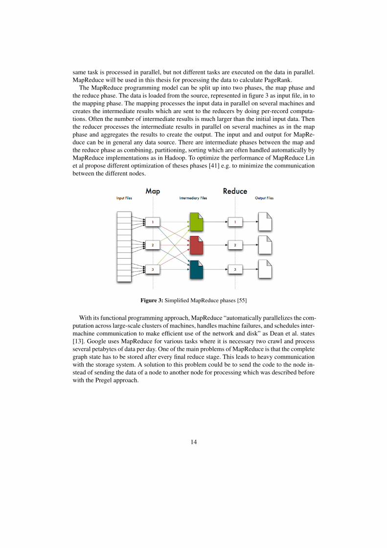
The MapReduce programming model can be split up into two phases, the map phase andthe reduce phase. The data is loaded from the source, represented in figure 3 as input file, in tothe mapping phase. The mapping processes the input data in parallel on several machines andcreates the intermediate results which are sent to the reducers by doing per-record computa-tions. Often the number of intermediate results is much larger than the initial input data. Thenthe reducer processes the intermediate results in parallel on several machines as in the mapphase and aggregates the results to create the output. The input and and output for MapRe-duce can be in general any data source. There are intermediate phases between the map andthe reduce phase as combining, partitioning, sorting which are often handled automatically byMapReduce implementations as in Hadoop. To optimize the performance of MapReduce Linet al propose different optimization of theses phases [41] e.g. to minimize the communicationbetween the different nodes.

Figure 3: Simplified MapReduce phases [55]

With its functional programming approach, MapReduce “automatically parallelizes the com-putation across large-scale clusters of machines, handles machine failures, and schedules inter-machine communication to make efficient use of the network and disk” as Dean et al. states[13]. Google uses MapReduce for various tasks where it is necessary two crawl and processseveral petabytes of data per day. One of the main problems of MapReduce is that the completegraph state has to be stored after every final reduce stage. This leads to heavy communicationwith the storage system. A solution to this problem could be to send the code to the node in-stead of sending the data of a node to another node for processing which was described beforewith the Pregel approach.

14

2.3 Storage systemsWith the growth of internet companies such as Google or Amazon and social platforms suchas Facebook or Twitter, new requirements for storage systems emerged. Google tries to storeand analyze as many webpages and links as possible to provide relevant search results. In2008, it already passed the mark of more than 1 trillion unique URLs [56]. Assuming everylink is 256 Bytes, only storing the links already equals 232 terabyte of storage. Twitter has tostore more than 90 million tweets per day [57] which is a large amount of data even if everytweet is only 140 characters long. Other kinds of so called big data are nowadays producedby location services (mobile phones) and sensor networks in general which are likely to growmassively in the next years [58]. The large amount of data makes it impossible to store andanalyze the data with a single machine or even a single cluster. Instead, it has to be distributed.With the need for new storage solutions, Google created BigTable [59] based on Google FileSystem (GFS) [60] and Amazon wrote the Dynamo paper [61] based on which SimpleDB andAmazon EC2 were implemented.

Also small companies are challenged by the big amount of data that is produced by its usersand by the social interactions. A new community, known as NoSQL (Not only SQL), grewand created different types of storage systems. Most are based on Dynamo (Riak) or BigTable(HBase) or a combination of both (Cassandra). One more solution that was developed byYahoo is PNUTS [62].

The main problem with current SQL solutions (MySQL, Oracle etc.) is that they are not easyto scale. Mainly, scaling writes and scaling queries to data sets stored and several machines.Current SQL solutions are often used as an all-purpose tool for everything. SQL solutions areperfect where a predefined data model exists, locking of entries is crucial, which means thatAtomicity, Consistency, Isolation, Durability (ACID) is necessary and transactions have to besupported. Often, the new solutions relax parts of ACID for better performance or scalability,and in the example of Dynamo also for eventual consistency. Other solutions keep all thedata in memory and only seldomly write their data on to disk. This makes them much moreefficient, but it could lead to data loss in case of a power outage or crash as long as the data isnot stored redundant.

There are use cases for every kind of system. All databases have to make tradeoffs at somepoint. Some of these tradeoffs are shown by the CAP theorem 2.3.1. There are systems thatare optimized for massive writes, others for massive reads. Most of these NoSQL solutions arestill in an early development phase, but they evolve fast and already found adaption in differenttypes of applications. The data models of the different solutions are diverse and optimized forthe use cases.

A switch from a SQL solution to one of the NoSQL solutions that were mentioned above isnot always easy or necessary. The storage model and structure varies from system to systemand querying data can be completely different by using MapReduce or so called views. Settingup these new solutions is often more complicated than simply installing a LAMP stack. SQLhas been developed for a long time and many packages have been created to simply copy it tothe hard drive to start working.

Most of the new storage systems were built so that they are able to run on several nodes toperform better, be fault tolerant and be accessible by different services, which means by a widevariety of programming languages. They offer interfaces like Representational State Transfer

15

(REST) [63] or Thrift [64] that allows easy access based on the standard HTTP Protocol overthe local network or the internet from various machines. The communication language canoften be chosen by the client. Standards as XML or JSON are supported. The efficiency of asystem differs on the use case and there is not a system that fits all needs. The no free lunchtheorem [65] can also be applied to storage systems.

Every system stores data differently. Data and queries have to be modeled differently forevery system so that they fit the underlying storage structure best. Depending on the systemand the use case, data has to be stored so that it can be queried as efficiently as possible. Mostsocial data sets have many to many relationships between the nodes which is a challenge inmost systems because it can not be represented naturally in the storage systems except forgraph databases.

To compare the performance of the different storage system types, Yahoo created Yahoo!Cloud Serving Benchmark (YCSB) [66]. This framework facilitates the performance com-parison of different cloud-based data storage systems. An other system to load-test variousdistributed storage system is vpork11 coming from the Voldemort project. Measuring perfor-mance is crucial for finding the right storage system but is not treated in this thesis becausethe focus lies on the data structure and not performance comparisons.

One goal of NoSQL solutions is massive scaling on demand. Thus, data can easily be dis-tributed on different computers without heavy interaction of the developer through a simpledeployment of additional nodes. The main challenge is to efficiently distribute the data on thedifferent machines and also to retrieve the data in an efficient way. In general, two differenttechniques are used: Sharding or distributed hash tables (DHT).

Sharding is used for horizontal partitioning when the data no longer fits on one machine.Based on the data ID, the data is stored on different system. As an example, all user IDsfrom 1 - 1000 are stored on one machine, all users from 1001 - 2000 are stored on the nextmachine. This is efficient for data that is not highly connected. With such data, queries can beanswered by one single machine. As soon as queries have to query and join data from differentmachines, sharding becomes inefficient. Scaling based on sharding is efficient for writes butcan be a bottleneck for queries. Sharding can use any kind of algorithms to distribute the dataon different nodes.

Distributed Hash Table (DHT) [67] is based on the idea of peer-to-peer, which distributesdata to the different nodes based on a hash key. DHT was implemented in 2001 in someprojects like Chord [68]. Nodes can dynamically join or leave the ring structure and data isreorganized automatically. The same data is stored on different nodes in order to guaranteeredundancy. This is of high value for the distributed storage systems, since machines in largeclusters regularly fail and have to be replaced without affecting or interrupting the rest of thecluster. Efficient algorithms help to find the data on the different nodes.

Even if most systems look completely new at first sight, most systems recombine existingfeatures. This is especially true for storage backends. Several distributed systems use well-known systems such as Oracle Berkley DB12 or InnoDB13 as storage backend on every node.These storage backends have proven to be stable and fast. They can often be exchanged in

11Distributed database load-testing utility: https://github.com/trav/vpork12Oracle Berkley DB: http://www.oracle.com/technetwork/database/berkeleydb/

overview/index.html13InnoDB: http://www.innodb.com/

16

order to optimize for a specific use case. Some systems allow the use of memory as storagebackend for faster reads and writes. However, with the disadvantage of loosing the data in caseof a crash.

In the following, first the technical details about the CAP Theorem, the Dynamo and theBigTable paper will be described. Then the five storage system types which are analyzed inthis thesis – as relational database management system, key-value store, column store, docu-ment store and graph databases – will be described in detail. So-called triple stores and quadstores like Hexastore [51] or RDF-3X [53] that were created and optimized to store, queryand search RDF triples, will not be analyzed because these storage systems are optimized forgraph matching and graph traversal queries but not for processing data. Object databases willneither be covered in this comparison because there were no popular object databases foundwhich are currently used for social data projects.

2.3.1 CAP, Dynamo and BigTable

Every storage system has its specific implementations. The next part will give a generaloverview of technical details that are used in various systems.

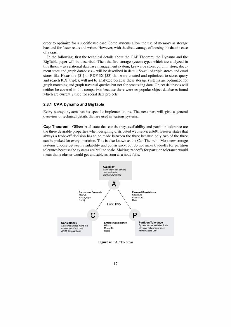
Cap Theorem Gilbert et al state that consistency, availability and partition tolerance arethe three desirable properties when designing distributed web services[69]. Brewer states thatalways a trade-off decision has to be made between the three because only two of the threecan be picked for every operation. This is also known as the Cap Theorem. Most new storagesystems choose between availability and consistency, but do not make tradeoffs for partitiontolerance because the systems are built to scale. Making tradeoffs for partition tolerance wouldmean that a cluster would get unusable as soon as a node fails.

ConsistencyAll clients always have the same view of the dataACID, Transactions

AvaibilityEach client can always read and writeTotal Redundancy

A

PC

Consensus ProtocolsMySQLHypergraphNeo4j

Eventual ConsistencyCouchDBCassandraRiak

Enforce ConsistencyHBaseMongoDbRedis

Partition ToleranceSystem works well despicete physical network partionsInfinite Scale Out

Pick Two

Figure 4: CAP Theorem

17

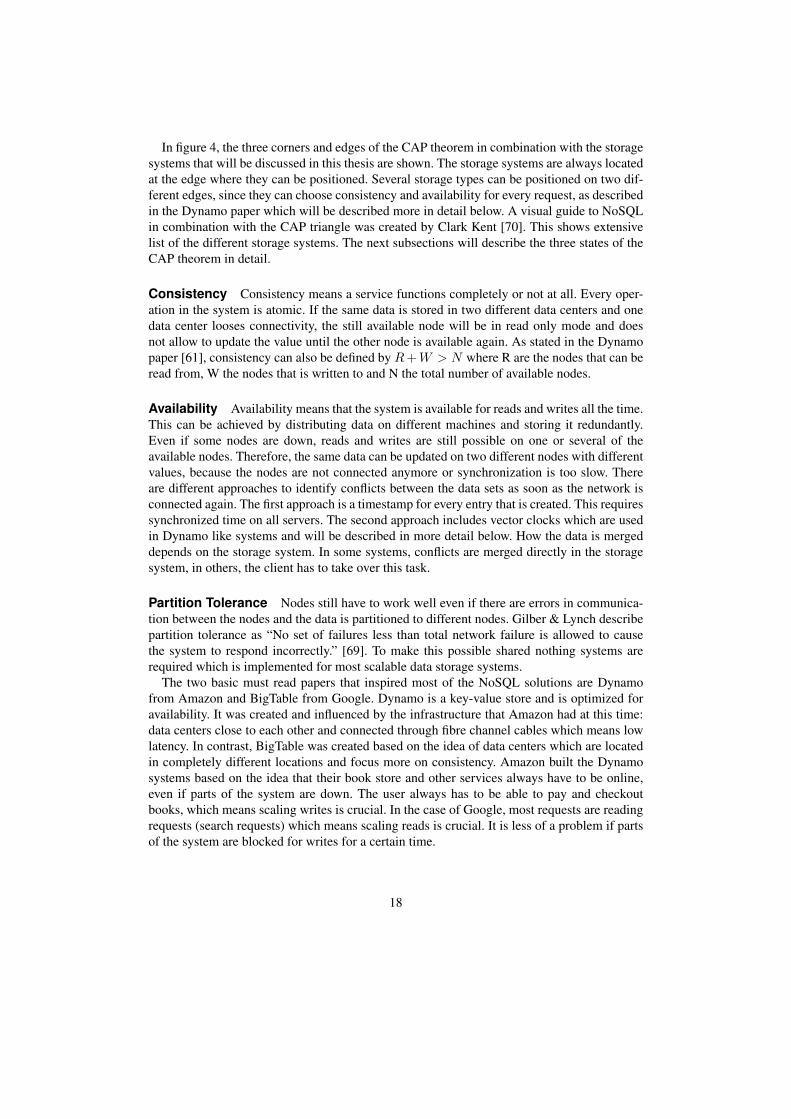
In figure 4, the three corners and edges of the CAP theorem in combination with the storagesystems that will be discussed in this thesis are shown. The storage systems are always locatedat the edge where they can be positioned. Several storage types can be positioned on two dif-ferent edges, since they can choose consistency and availability for every request, as describedin the Dynamo paper which will be described more in detail below. A visual guide to NoSQLin combination with the CAP triangle was created by Clark Kent [70]. This shows extensivelist of the different storage systems. The next subsections will describe the three states of theCAP theorem in detail.

Consistency Consistency means a service functions completely or not at all. Every oper-ation in the system is atomic. If the same data is stored in two different data centers and onedata center looses connectivity, the still available node will be in read only mode and doesnot allow to update the value until the other node is available again. As stated in the Dynamopaper [61], consistency can also be defined by R + W > N where R are the nodes that can beread from, W the nodes that is written to and N the total number of available nodes.

Availability Availability means that the system is available for reads and writes all the time.This can be achieved by distributing data on different machines and storing it redundantly.Even if some nodes are down, reads and writes are still possible on one or several of theavailable nodes. Therefore, the same data can be updated on two different nodes with differentvalues, because the nodes are not connected anymore or synchronization is too slow. Thereare different approaches to identify conflicts between the data sets as soon as the network isconnected again. The first approach is a timestamp for every entry that is created. This requiressynchronized time on all servers. The second approach includes vector clocks which are usedin Dynamo like systems and will be described in more detail below. How the data is mergeddepends on the storage system. In some systems, conflicts are merged directly in the storagesystem, in others, the client has to take over this task.

Partition Tolerance Nodes still have to work well even if there are errors in communica-tion between the nodes and the data is partitioned to different nodes. Gilber & Lynch describepartition tolerance as “No set of failures less than total network failure is allowed to causethe system to respond incorrectly.” [69]. To make this possible shared nothing systems arerequired which is implemented for most scalable data storage systems.

The two basic must read papers that inspired most of the NoSQL solutions are Dynamofrom Amazon and BigTable from Google. Dynamo is a key-value store and is optimized foravailability. It was created and influenced by the infrastructure that Amazon had at this time:data centers close to each other and connected through fibre channel cables which means lowlatency. In contrast, BigTable was created based on the idea of data centers which are locatedin completely different locations and focus more on consistency. Amazon built the Dynamosystems based on the idea that their book store and other services always have to be online,even if parts of the system are down. The user always has to be able to pay and checkoutbooks, which means scaling writes is crucial. In the case of Google, most requests are readingrequests (search requests) which means scaling reads is crucial. It is less of a problem if partsof the system are blocked for writes for a certain time.

18

Dynamo allows to choose for every request (read / write / delete) how many nodes shouldbe queried or written to. Thus, the CAP theorem axis can be different for every request. Thisenables the developer to decide how redundantly data should be stored. The assumption ismade if data is written to for example at least three servers out of five, the data is consistent.This is known as eventual consistency. Still it is possible that different versions of a data setexist on different servers. To differentiate between this different versions Dynamo uses vectorclocks [71]. To handle temporary failures, the so-called sloppy quorum approach is used:Instead of using the traditional approach, data can be read and written to the first N healthynodes instead of writing to the three predefined nodes. Otherwise it would be unavailableduring server failures.

2.3.2 Relational database management system (RDBMS)

Relational database management systems are probably the storage systems that are at themoment used the most often. Data is modeled in tables consisting of predefined columns, thedata itself is stored in rows. The data structure is often created based on the five normal formswhich are designed to prevent update anomalies [72]. To query data that is stored in two tables,joins are necessary. For storing and querying structured data with a predefined model that isnot changing, RDBMS are suitable. For every column indices can be set. Retrieving data basedin indices is efficient and fast. Inserting data is also fast and efficient because only a row hasto be inserted and the corresponding indices (often B+ trees) updated.

One of the main disadvantages of relational databases is that when data grows, joins becomemore and more expensive because lots of data has to be queried in order to create the results.As soon as joins become larger than the memory size or have to be processed on more thanone machine, these joins are getting more and more inefficient the larger and more distributedthe data gets.

In the area of RDBMS there is recently also a lot of development and also new RDBMS likeVoltDB14 appeared on the market that promise to be more scalable and still support ACIDityand transactions.

Popular RDBMS are MySQL 3.3.1, PostgreSQL15, SQLite16 or Oracle Database17. In thisthesis, MySQL is used for the analysis.

2.3.3 Key-value stores

The simplest way to store data is with key-value store. Keys are normally strings, valuescan be any type of objects (binary data). Most key-value stores are similar to the popularmemached [73] cache but add a persistence layer in the backend. The range of available key-value stores ranges from simple single list key-value stores to support for lists, ordered lists(Redis) or storing complete documents (Riak). Key-value stores are optimized for heavy readsand writes but only offer minimal querying functionality. The Dynamo implementation forexample is basically a key-value store implementation that was implemented as SimpleDB.

14Scalable Open Source RDBMS http://voltdb.com/15PostgreSQL: http://www.postgresql.org/16Server-less SQL database http://www.sqlite.org/17Oracle Database: http://www.oracle.com/de/products/database/index.html

19

Modeling complex data for key-value stores is often more complicated because pure key-values stores only support fetching values by keys. No secondary indices are supported. Tostore and retrieve data, combined key names are often used to make the keys unique andto make it possible to retrieve values again. The basic system does not support any querymechanism or indicies. Because of their simplicity, key-value stores are often used as cachinglayer.

Popular key-value stores are SimpleDB18, Redis 3.3.2, membase19, Riak 3.3.3 or TokyoTyrant 20. For the experiments Redis and Riak are used.

2.3.4 Column stores

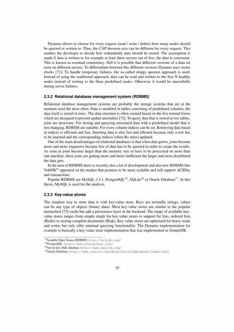
In Column stores, data is stored in columns – as opposed to the rows that are used in relationalor row oriented database systems. With column stores it is possible to store similar data (thatbelongs to one row) close to each other on disk. Is is not necessary to predefine how muchcolumns will be in one row. One of the first implementations in research was C-Store [74],which was created as a collaboration project among different universities.

Cassandra and HBase are based on BigTable[59], which is a standard column store im-plementation by Google. BigTable is used at Google for almost all their applications suchsearch, Google Docs or Google Calendar. For scaling, Google uses the Google File System(GFS) [60]. Figure 5 is an example of how Google stores its search data in a BigTable. Alldata related to www.cnn.com is stored in one row. In the first column content, the webpagecontent is stored. In the other columns, all website URLs which have an anchor / URL towww.cnn.com are stored. This data is stored closely together on disk. For processing the datafor www.cnn.com, the system has to retrieve only one row of data.Bigtable: A Distributed Storage System for Structured Data · 4: 3

Fig. 1. A slice of an example table that stores Web pages. The row name is a reversed URL. Thecontents column family contains the page contents, and the anchor column family contains thetext of any anchors that reference the page. CNN’s home page is referenced by both the SportsIllustrated and the MY-look home pages, so the row contains columns named anchor:cnnsi.comand anchor:my.look.ca. Each anchor cell has one version; the contents column has three versions,at timestamps t3, t5, and t6.

balancing, and columns are grouped together to form the unit of access controland resource accounting.

We settled on this data model after examining a variety of potential uses ofa Bigtable-like system. Consider one concrete example that drove many of ourdesign decisions: a copy of a large collection of web pages and related informa-tion that could be used by many different projects. Let us call this particulartable the Webtable. In Webtable, we would use URLs as row keys, various as-pects of web pages as column names, and store the contents of the web pagesin the contents: column under the timestamps when they were fetched, asillustrated in Figure 1.

Rows. Bigtable maintains data in lexicographic order by row key. The rowkeys in a table are arbitrary strings (currently up to 64KB in size, although10-100 bytes is a typical size for most of our users). Every read or write ofdata under a single row key is serializable (regardless of the number of differ-ent columns being read or written in the row), a design decision that makesit easier for clients to reason about the system’s behavior in the presence ofconcurrent updates to the same row. In other words, the row is the unit oftransactional consistency in Bigtable, which does not currently support trans-actions across rows.

Rows with consecutive keys are grouped into tablets, which form the unitof distribution and load balancing. As a result, reads of short row rangesare efficient and typically require communication with only a small numberof machines. Clients can exploit this property by selecting their row keys sothat they get good locality for their data accesses. For example, in Webtable,pages in the same domain are grouped together into contiguous rows byreversing the hostname components of the URLs. We would store data formaps.google.com/index.html under the key com.google.maps/index.html. Stor-ing pages from the same domain near each other makes some host and domainanalyses more efficient.

Columns. Column keys are grouped into sets called column families, whichform the unit of access control. All data stored in a column family is usuallyof the same type (we compress data in the same column family together). Acolumn family must be created explicitly before data can be stored under any

ACM Transactions on Computer Systems, Vol. 26, No. 2, Article 4, Pub. date: June 2008.

Figure 5: Column store

Column stores are built with the idea of scaling in mind. There are only few indices, mostbased on the row keys. Also, data is directly sorted and stored based on the row keys as in BigTable. This makes it efficient to retrieve data that is close to each other. There is no specificquery language. Some column stores only allow to retrieve documents based on the row keyor to make range queries for row keys. Some support more advanced query methods but notwith a standardized query language.

18Key-value store based on the Dynamo paper: http://aws.amazon.com/simpledb/19Simple key-value store based on memcached http://membase.org/20Tokyo Tyrant: network interface of Tokyo Cabinet: http://fallabs.com/tokyotyrant/

20

Popular column stores are BigTable, Voldemort21, HBase 3.3.6, Hypertable or Cassandra3.3.7. In this thesis, Cassandra and HBase are used for the analysis.

2.3.5 Document stores

In document stores, records are stored in the form of documents. Normally, the structure andform of the data does not have to be predefined. The type and structure of the fields can differbetween every document. Every stored document has a unique id to retrieve or update the doc-ument. The stored data is semi-structured which means that there is no real separation betweendata and schema. Thus, the model can change dynamically. Depending on the system valuesinside a document can be typed. Several document stores support storing the data directly asJSON documents. This facilitates the creating and retrieving of documents. Similar types ofdocuments or documents with similar structures can be stored under buckets or databases.Normally, the storage systems automatically create a unique identifier for every document, butthis identifier can also set by the client.

Document stores offer much comfort for the programmer because data can directly be storedin the structure it is. Thus, data does not have to be normalized first, and programmers do notneed to worry about a structure that might or might not be supported by the database system.

To query data efficiently, some data stores support indices over predefined values insidethe documents. There is no standard query language. Also systems have different strategiesof querying the data. There are two different approaches to scale document stores. One issharding, already known from the RDBMS. The documents are distributed on different serverbased on the ID. Also queries for documents have to be made on the specific servers. An otherapproach is based on the Dynamo paper. This says that documents are distributed based on aDHT on different servers. There is for example an approach to implement the storage backendof CouchDB based on Dynamo [75].

Popular document stores are MongoDB 3.3.4, CouchDB 3.3.5 or RavenDB22. In this thesis,CouchDB and MongoDB are used for the analysis.

2.3.6 Graph databases

In comparison to other storage systems, graph databases store the data as a graph instead ofjust representing a graph structure. Marko A. Rodriguez defines graph databases in a moretechnical way: “A graph database is any storage system that provides index-free adjacency”[76]. According to Rodriguez, moving from one adjacent vertex to the next always takes thesame amount of time – regardless where in the graph the vertex is, how many vertices there areand without using indices. In other databases, an index would be needed to determine whichvertices are adjacent to a vertex.

General graph databases such as Neo4j are optimized for graph traversal. Other typicalgraph application patterns are scoring, ranking and search. Triple and quad stores that areoften used for storing and querying RDF data are no typical graph databases. Theses systemsare optimized for graph matching queries to match subject, predicates and object and can oftenbe used with the SPARQL [5] query language. There are also several different approaches to

21A distributed database http://project-voldemort.com/22RavenDB: http://ravendb.net/

21

build graph databases based on existing databases such as for example FlockDB [77] which isbased on MySQL, created by Twitter. These types of graph databases are often optimized fora concrete use case.

There are different query languages for graph databases. In the area of RDF stores, SPARQL[5] is the de-facto standard. Gremlin [78] uses another approach, which is optimized for prop-erty graphs23. Current graph databases often have their own implementations of a query ortraversal language that is optimized for the storage system. In addition, the default query lan-guage SPARQL is often supported.

At the moment, graph databases evolve fast. New databases appear on the market, most ofthem with the goal of being more scalable and distributed, such as for example InfoGrid24 orInfiniteGraph.

Popular graph databases are Neo4j 3.3.8, HypergraphDB25, AllegroGraph26, FlockDB [77]or Inifinite Graph27. In this thesis, Neo4j is used for the analysis. HypergraphDB was alsoconsidered, but Neo4j seems to have a simpler implementation, is more extensible and has abetter documentation than HypergraphDB.

2.4 Data visualizationData or information visualization means a graphical representation of data that is mostly gener-ated by computers [14]. The goal of data visualization is to convert data to a meaningful graph[14] and make it unterstandable for people to communicate complex ideas and to gain insightsinto the data. Both art and science are part of data visualization. Shneidermann defined a taskby data type taxonomy based on the Visual Information-Seeking Matra (overview first, zoomand filter, then details on demand) with seven data types and seven tasks [79]. Graph drawingis not only based on mathematical rules, but it also has to respect aesthetic rules: Minimaledge crossing, evenly distributed vertices and symmetry have to be taken into account [15]. Itis important to find a good visual representation for the data that can be understood by people.There are different graph drawing models and algorithms. One often used method is the springelectrical model, which is scalable to thousands of vertices. Other approaches are the stressmodel or the minimal energy model[15].

Hu describes the visualization problem as following [16]:

The key enabling ingredients include a multilevel approach, force approximationsby space decomposition and algebraic techniques for the robust solution of thestress model and in the sparsification of it.

One of the general problems in data visualization is that many graphs are too large to beprocessed on a single machine. To solve this, some graph partitioning and community detec-tion algorithms [80] have to be used, namely the parallel algorithms that were proposed byMadduri and Bader [81] [11].

23Property graph defined by blueprint: http://github.com/tinkerpop/blueprints/wiki/property-graph-model

24InfoGrid Web Graph Database: http://infogrid.org/25HypergraphDB project: http://www.kobrix.com/hgdb.jsp26Proprietary RDF store: http://www.franz.com/agraph/allegrograph/27Distributed Graph Database: http://www.infinitegraph.com/

22

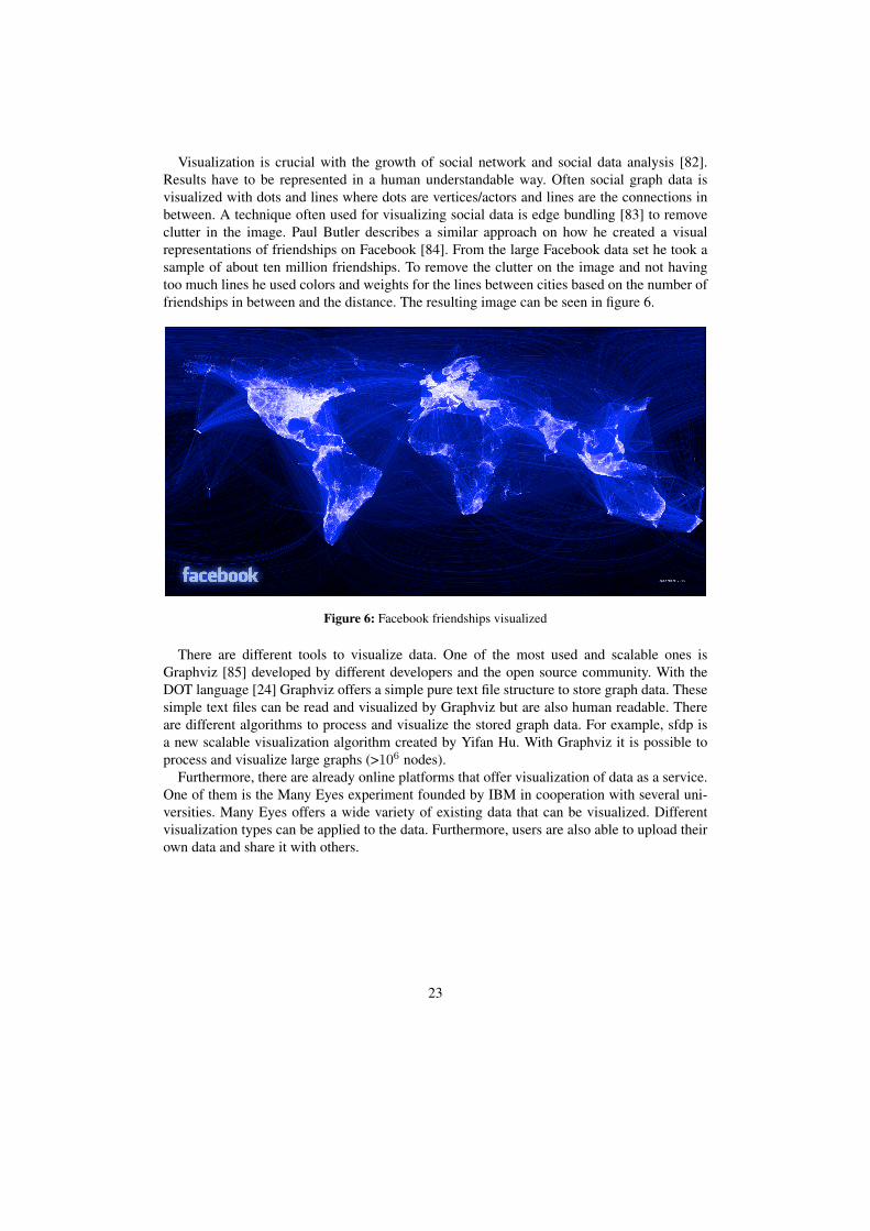
Visualization is crucial with the growth of social network and social data analysis [82].Results have to be represented in a human understandable way. Often social graph data isvisualized with dots and lines where dots are vertices/actors and lines are the connections inbetween. A technique often used for visualizing social data is edge bundling [83] to removeclutter in the image. Paul Butler describes a similar approach on how he created a visualrepresentations of friendships on Facebook [84]. From the large Facebook data set he took asample of about ten million friendships. To remove the clutter on the image and not havingtoo much lines he used colors and weights for the lines between cities based on the number offriendships in between and the distance. The resulting image can be seen in figure 6.

Figure 6: Facebook friendships visualized

There are different tools to visualize data. One of the most used and scalable ones isGraphviz [85] developed by different developers and the open source community. With theDOT language [24] Graphviz offers a simple pure text file structure to store graph data. Thesesimple text files can be read and visualized by Graphviz but are also human readable. Thereare different algorithms to process and visualize the stored graph data. For example, sfdp isa new scalable visualization algorithm created by Yifan Hu. With Graphviz it is possible toprocess and visualize large graphs (>106 nodes).

Furthermore, there are already online platforms that offer visualization of data as a service.One of them is the Many Eyes experiment founded by IBM in cooperation with several uni-versities. Many Eyes offers a wide variety of existing data that can be visualized. Differentvisualization types can be applied to the data. Furthermore, users are also able to upload theirown data and share it with others.

23

3 Data, Methods & ImplementationFor the analysis of social network data and the implementation of the centrality algorithm, aspecific data set was needed. The useKit data set from the social ad-hoc collaboration plat-form useKit.com was chosen. The data was modeled for the following eight storage systems:MySQL, Redis, Riak, MongoDB, CouchDB, HBase, Cassandra and Neo4j. The data modelwas specifically created and adapted for every single system. To calculate degree centralityand PageRank on the different storage systems, the useKit data set first had to be stored inevery system. Then, the degree centrality and PageRank algorithms where implemented onevery system if possible. To better understand the global structure of the network, the data wasvisualized with the help of Graphviz.

In the following, first the exact structure of the useKit data will be described in detail,followed by a description of what the concrete algorithms of degree centrality and PageRanklook like. Then, all eight storage systems and their technical background will be described indetail. Last, methods of visualizing network data are described.

3.1 useKit DataSocial data cannot be created simply by connecting random nodes through edges, becausesocial networks are often small world networks. There are different methods to create thesekinds of networks, such as the preferential attachment method proposed by Barabasi et al[86]. To not rely on randomly created data, a data set from the social ad-hoc collaborationplatform useKit.com28 was taken. The decision was made for the useKit data set because ofthe direct connection to the useKit team, the willingness of the useKit team to provide the dataset and because other available social data sets are rare as described in section 2.1.3. useKit isa platform that offers organization of content combined with simple collaboration. The useKitdata structure was simplified to its basics. Additional nodes such as comments or likes wereneglected. The simplified data consists of three different types of nodes: Content, context anduser, as can be seen in figure 7. Every node type is described below.

Content Every content item produced by a user in the useKit platform is stored as a contentnode. A content item can be a link, video, file or every other type of data that can be stored inuseKit. Every content object is created by a user. Thus, this user is the creator of the createdcontent object. In addition, several users can own the content object. This means that theseusers have a symlink to the same content item. A content item exists in the system as long asat least one symlink to the content item exists. These links are the edges between content nodesand user nodes. Because at least one user has to own the object but the number of owners isunlimited, this represents a 1 to N relation which is shown in figure 7. All content items canbe in several contexts, but they do not have to be. This equals a 0 to N relation between thecontent and the context nodes. A content item is indirectly related to other content items overcontexts or users. This means that if a content item is in the same context as another contentobject or the same user owns two content objects, there is an indirect relation between thesetwo content objects.

28useKit Platform: http://useKit.com

24

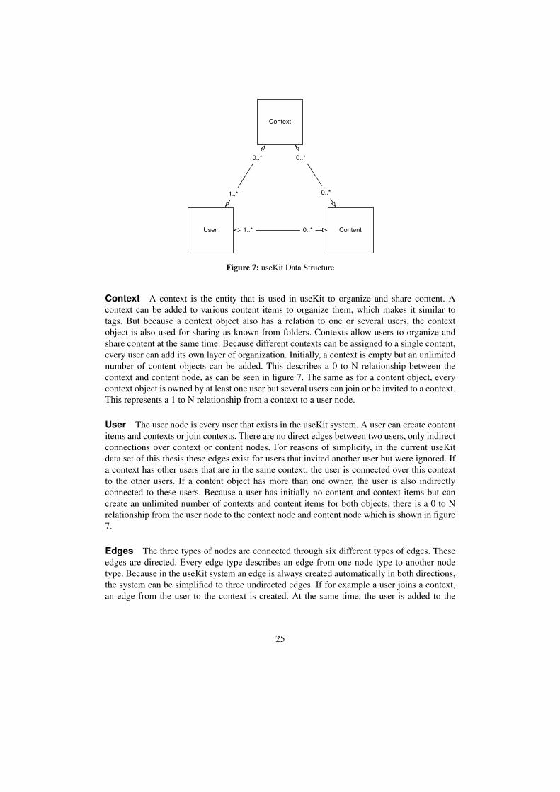
User

Context

Content

0..*

1..*

0..*

0..*

1..* 0..*

Figure 7: useKit Data Structure

Context A context is the entity that is used in useKit to organize and share content. Acontext can be added to various content items to organize them, which makes it similar totags. But because a context object also has a relation to one or several users, the contextobject is also used for sharing as known from folders. Contexts allow users to organize andshare content at the same time. Because different contexts can be assigned to a single content,every user can add its own layer of organization. Initially, a context is empty but an unlimitednumber of content objects can be added. This describes a 0 to N relationship between thecontext and content node, as can be seen in figure 7. The same as for a content object, everycontext object is owned by at least one user but several users can join or be invited to a context.This represents a 1 to N relationship from a context to a user node.

User The user node is every user that exists in the useKit system. A user can create contentitems and contexts or join contexts. There are no direct edges between two users, only indirectconnections over context or content nodes. For reasons of simplicity, in the current useKitdata set of this thesis these edges exist for users that invited another user but were ignored. Ifa context has other users that are in the same context, the user is connected over this contextto the other users. If a content object has more than one owner, the user is also indirectlyconnected to these users. Because a user has initially no content and context items but cancreate an unlimited number of contexts and content items for both objects, there is a 0 to Nrelationship from the user node to the context node and content node which is shown in figure7.

Edges The three types of nodes are connected through six different types of edges. Theseedges are directed. Every edge type describes an edge from one node type to another nodetype. Because in the useKit system an edge is always created automatically in both directions,the system can be simplified to three undirected edges. If for example a user joins a context,an edge from the user to the context is created. At the same time, the user is added to the

25

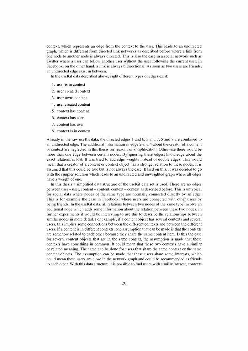
context, which represents an edge from the context to the user. This leads to an undirectedgraph, which is different from directed link networks as described before where a link fromone node to another node is always directed. This is also the case in a social network such asTwitter where a user can follow another user without the user following the current user. InFacebook, on the other hand, a link is always bidirectional. As soon as two users are friends,an undirected edge exist in between.

In the useKit data described above, eight different types of edges exist:

1. user is in context

2. user created context

3. user owns content

4. user created content

5. context has content

6. context has user

7. content has user

8. context is in context

Already in the raw useKit data, the directed edges 1 and 6, 3 and 7, 5 and 8 are combined toan undirected edge. The additional information in edge 2 and 4 about the creator of a contentor context are neglected in this thesis for reasons of simplification. Otherwise there would bemore than one edge between certain nodes. By ignoring these edges, knowledge about theexact relations is lost. It was tried to add edge weights instead of double edges. This wouldmean that a creator of a content or context object has a stronger relation to these nodes. It isassumed that this could be true but is not always the case. Based on this, it was decided to gowith the simpler solution which leads to an undirected and unweighted graph where all edgeshave a weight of one.

In this thesis a simplified data structure of the useKit data set is used. There are no edgesbetween user – user, content – content, context – context as described before. This is untypicalfor social data where nodes of the same type are normally connected directly by an edge.This is for example the case in Facebook, where users are connected with other users bybeing friends. In the useKit data, all relations between two nodes of the same type involve anadditional node which adds some information about the relation between these two nodes. Infurther experiments it would be interesting to use this to describe the relationships betweensimilar nodes in more detail. For example, if a content object has several contexts and severalusers, this implies some connections between the different contexts and between the differentusers. If a content is in different contexts, one assumption that can be made is that the contextsare somehow related to each other because they share the same content item. Is this the casefor several content objects that are in the same context, the assumption is made that thesecontexts have something in common. It could mean that these two contexts have a similaror related meaning. The same can be done for users that share the same context or the samecontent objects. The assumption can be made that these users share some interests, whichcould mean these users are close in the network graph and could be recommended as friendsto each other. With this data structure it is possible to find users with similar interest, contexts

26

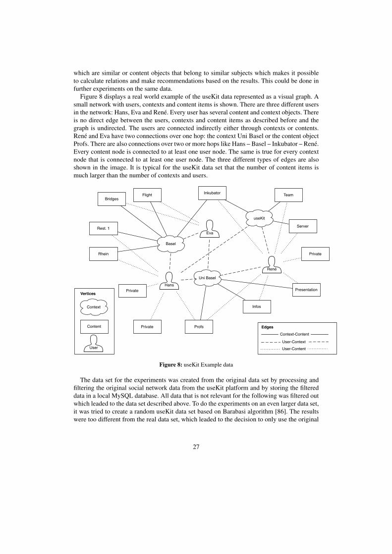
which are similar or content objects that belong to similar subjects which makes it possibleto calculate relations and make recommendations based on the results. This could be done infurther experiments on the same data.

Figure 8 displays a real world example of the useKit data represented as a visual graph. Asmall network with users, contexts and content items is shown. There are three different usersin the network: Hans, Eva and René. Every user has several content and context objects. Thereis no direct edge between the users, contexts and content items as described before and thegraph is undirected. The users are connected indirectly either through contexts or contents.René and Eva have two connections over one hop: the context Uni Basel or the content objectProfs. There are also connections over two or more hops like Hans – Basel – Inkubator – René.Every content node is connected to at least one user node. The same is true for every contextnode that is connected to at least one user node. The three different types of edges are alsoshown in the image. It is typical for the useKit data set that the number of content items ismuch larger than the number of contexts and users.

Basel

Rhein

Rest. 1

BridgesFlight

Uni BaselHans

Inkubator Team

Profs

Infos

Presentation

René

Eva

Private

Server

useKit

Private

Private

Context

Vertices

Content

User

Context-Content

User-ContextUser-Content

Edges

Figure 8: useKit Example data

The data set for the experiments was created from the original data set by processing andfiltering the original social network data from the useKit platform and by storing the filtereddata in a local MySQL database. All data that is not relevant for the following was filtered outwhich leaded to the data set described above. To do the experiments on an even larger data set,it was tried to create a random useKit data set based on Barabasi algorithm [86]. The resultswere too different from the real data set, which leaded to the decision to only use the original

27

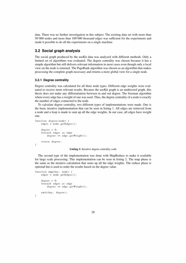
data. There was no further investigation in this subject. The existing data set with more than50’000 nodes and more than 100’000 thousand edges was sufficient for the experiments andmade it possible to do all the experiments on a single machine.

3.2 Social graph analysisThe social graph produced by the useKit data was analyzed with different methods. Only alimited set of algorithms was evaluated. The degree centrality was chosen because it has asimple algorithm but still delivers relevant information in most cases even though only a localview on the node is returned. The PageRank algorithm was chosen as an algorithm that makesprocessing the complete graph necessary and returns a more global view for a single node.

3.2.1 Degree centrality

Degree centrality was calculated for all three node types. Different edge weights were eval-uated to receive more relevant results. Because the useKit graph is an undirected graph, thisthesis does not make any differentiation between in and out degree. The freeman algorithmwhere every edge has a weight of one was used. Thus, the degree centrality of a node is exactlythe number of edges connected to the node.

To calculate degree centrality, two different types of implementations were made. One isthe basic iterative implementation that can be seen in listing 1. All edges are retrieved froma node and a loop is made to sum up all the edge weights. In our case, all edges have weightone.

f u n c t i o n d e g r e e ( node ) {edges = node . g e t E d g e s ( ) ;

d e g r e e = 0 ;f o r e a c h edges as edge

d e g r e e += edge . ge tWeigh t ( ) ;

r e t u r n d e g r e e ;}

Listing 1: Iterative degree centrality code

The second type of the implementation was done with MapReduce to make it availablefor large scale processing. This implementation can be seen in listing 2. The map phase isthe same as the iterative calculation that sums up all the edge weights. The reduce phase isoptional but is used to order the results based on the degree value.

f u n c t i o n map ( key , node ) {edges = node . g e t E d g e s ( ) ;

d e g r e e = 0 ;f o r e a c h edges as edge

d e g r e e += edge . ge tWeigh t ( ) ;

emi t ( key , d e g r e e ) ;}

28

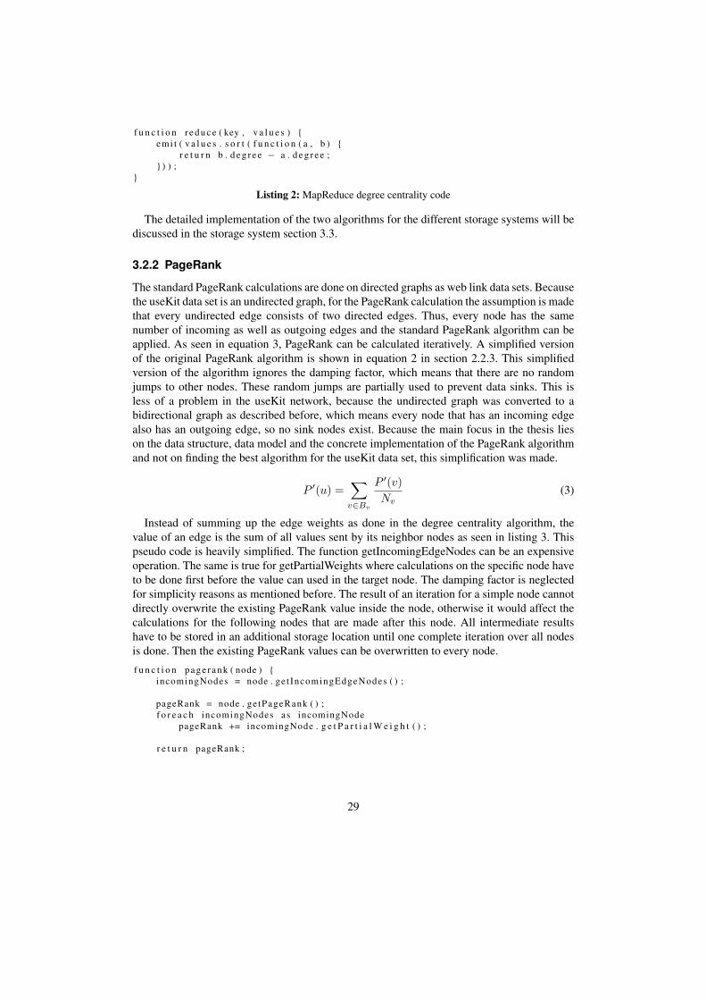
f u n c t i o n r e d u c e ( key , v a l u e s ) {emi t ( v a l u e s . s o r t ( f u n c t i o n ( a , b ) {

r e t u r n b . d e g r e e − a . d e g r e e ;} ) ) ;

}

Listing 2: MapReduce degree centrality code

The detailed implementation of the two algorithms for the different storage systems will bediscussed in the storage system section 3.3.

3.2.2 PageRank

The standard PageRank calculations are done on directed graphs as web link data sets. Becausethe useKit data set is an undirected graph, for the PageRank calculation the assumption is madethat every undirected edge consists of two directed edges. Thus, every node has the samenumber of incoming as well as outgoing edges and the standard PageRank algorithm can beapplied. As seen in equation 3, PageRank can be calculated iteratively. A simplified versionof the original PageRank algorithm is shown in equation 2 in section 2.2.3. This simplifiedversion of the algorithm ignores the damping factor, which means that there are no randomjumps to other nodes. These random jumps are partially used to prevent data sinks. This isless of a problem in the useKit network, because the undirected graph was converted to abidirectional graph as described before, which means every node that has an incoming edgealso has an outgoing edge, so no sink nodes exist. Because the main focus in the thesis lieson the data structure, data model and the concrete implementation of the PageRank algorithmand not on finding the best algorithm for the useKit data set, this simplification was made.

P ′(u) =∑

v∈Bv

P ′(v)Nv

(3)

Instead of summing up the edge weights as done in the degree centrality algorithm, thevalue of an edge is the sum of all values sent by its neighbor nodes as seen in listing 3. Thispseudo code is heavily simplified. The function getIncomingEdgeNodes can be an expensiveoperation. The same is true for getPartialWeights where calculations on the specific node haveto be done first before the value can used in the target node. The damping factor is neglectedfor simplicity reasons as mentioned before. The result of an iteration for a simple node cannotdirectly overwrite the existing PageRank value inside the node, otherwise it would affect thecalculations for the following nodes that are made after this node. All intermediate resultshave to be stored in an additional storage location until one complete iteration over all nodesis done. Then the existing PageRank values can be overwritten to every node.

f u n c t i o n p a g e r a n k ( node ) {incomingNodes = node . ge t IncomingEdgeNodes ( ) ;

pageRank = node . ge tPageRank ( ) ;f o r e a c h incomingNodes as incomingNode

pageRank += incomingNode . g e t P a r t i a l W e i g h t ( ) ;

r e t u r n pageRank ;

29

}

Listing 3: PageRank iterative pseudo code

MapReduce at Google was developed to scale the PageRank algorithm to billions of web-sites. The pseudocode for the map and the reduce phase can be found in listing 4. In the mapphase, first the current PageRank value of the node is divided by the number of incomingedges. The resulting value is the amount that is sent to each connected node in the secondpart of the map phase. In the reduce phase, all these partial values sent for a single node aresummed up and stored as new PageRank value. Detailed optimization proposals for this algo-rithm can be found in “Design Patterns for Efficient Graph Algorithms in MapReduce” fromLin and Schatz[41]. PageRank is an algorithm that converges after multiple iterations. Thesize of the graph only slightly affects the number of iterations, often ten iterations are alreadyenough for a good approximation of the exact PageRank [87]. For multiple attached iterationsof the PageRank algorithms it is necessary to also emit the complete node information dur-ing the map phase. Then all information that is necessary for several map and reduce phasesdirectly exists inside the system. This allows us to repeat the PageRank calculation severaltimes. Would the node not be sent, the node information like connected nodes would be lostand multiple iterations would no be possible without accessing the storage system.f u n c t i o n map ( key , node ) {

p a r t i a l P a g e R a n k V a l u e = node . PageRank / # node . a d j a c e n c y L i s t ;

f o r e a c h node . a d j a c e n c y L i s t a s ad jacencyNodeemi t ( ad jacencyNode . id , p a r t i a l P a g e n R a n k V a l u e ) ;

}

f u n c t i o n r e d u c e ( key , v a l u e s ) {pageRank = 0 ;

f o r e a c h v a l u e s a s v a l u epageRank += v a l u e ;

emi t ( key , pageRank ) ;}

Listing 4: PageRank MapReduce code

The detailed implementation for every specific storage system can be found in the section3.3. Depending on the system, the iterative or the MapReduce implementation was chosen.

3.3 Storage systems and their data modelsSince the amount of data is growing, there is a need for new storage systems. The numberof different so-called Not only SQL (NoSQL) solutions is growing fast. Thus, in the courseof writing this thesis, new systems appeared and the analyzed systems evolved and were im-proved. During the next years, probably only the best and most stable systems will further bedeveloped and it is likely to become easier to choose the right system for a specific problem.The current development pace for NoSQL solutions is quite high. While writing this thesis,Redis evolved from version 1.0 to version 2.2, several features were added and the speed im-proved. This fast development pace has lead to confusion in the communities because there

30

are many blog entries or outdated documentations where old systems are compared without aspecific version number.

The storage systems which are analyzed in this thesis were chosen based on the followingfactors: Documentation, usage in projects, community behind the project, stability, active de-velopment, open source, available clients and my personal assessment. All the chosen systemsare open source. This was an important basis for decision, because it makes it possible toevaluate the systems in detail by studying and analyzing the code when needed. One or twosystems of every type were chosen to compare the results and also to guarantee that at leastone solution still exists at the end of writing this thesis. One more reason to pick more than onesolution per type was that there are completely different implementations for the same type, ascan be seen with Riak and Redis that are basically both key-value stores but have completelydifferent implementations. New systems appeared during writing, which are mentioned belowbut not evaluated in detail. The systems were selected in July 2010.

For simplicity it was decided to make all client implementations in Java. Java was chosenbecause all storage systems offer a Java client or have a Java API by default. In addition, Javaallows us to make the written code cross platform executable. The specific clients that werechosen for the individual storage system are listed in the description of every storage systembelow. The communication between the client and the server depended on the server, but mostsystems have REST interface and support communication through JSON, which was also usedfor data modeling.

The data was modeled for every single storage system to store, query and process the data inan adequate way. For most storage systems, the data had to be denormalized. The advantage ofthis approach is that data is stored in a way that is ideal to query the data, the disadvantage isthat much duplicated data exists in the system and the programmer has to take care of removingduplicated or outdated data which is more a fat client – thin server architecture approach.

In table 1 an overview of the eight evaluated systems can be found where storage type,implementation code language and supported query languages are listed. For a more extensivelist of storage systems, Knut Haugen created a blog entry with Google Docs that lists moredetails [88]. All storage systems support simple key requests based on an index, except Neo4jwhere this can be added through a Lucene29 index. The storage systems are written in differentlanguages. In this context, Erlang30 – as a functional programming language built to createdistributed, fault-tolerant systems – should be mentioned. It seems as if Erlang is a good matchfor distributed systems such as Riak.

In the following, all eight storage systems are described in detail. The initial data set wasstored in MySQL. To feed all the other systems with data, scripts were created to query thedata from the MySQL database, remodel the data and write it into the specific storage system.

3.3.1 MySQL

MySQL31 is probably the most popular relational open source database. It is used in a widevariety of projects and has proven to be stable. Because of its easy installation and setup itis used in lots of small projects, but also in large production environments as for example

29Lucene project: http://lucene.apache.org/java/docs/index.html30Erlang a functional programming language: http://www.erlang.org/31MySQL webpage: http://www.mysql.com/

31

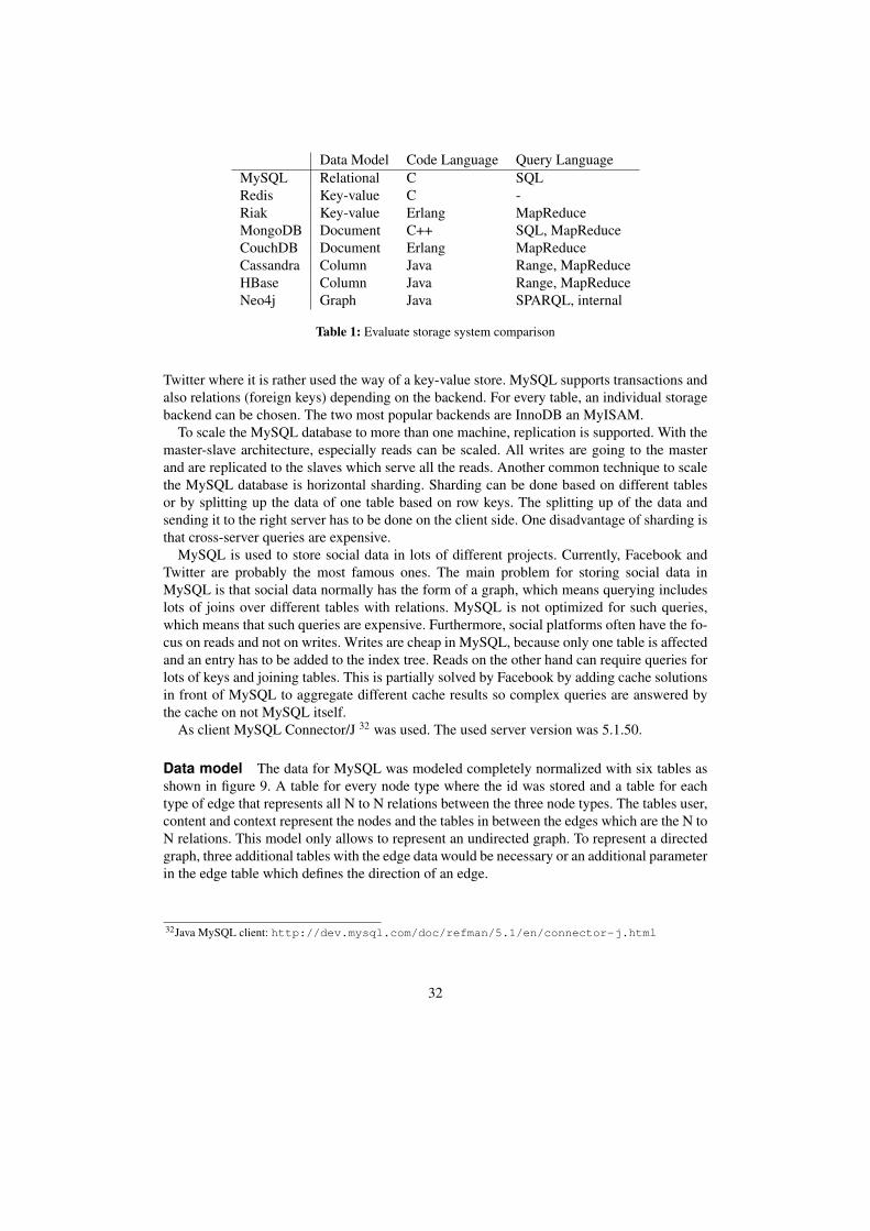
Data Model Code Language Query LanguageMySQL Relational C SQLRedis Key-value C -Riak Key-value Erlang MapReduceMongoDB Document C++ SQL, MapReduceCouchDB Document Erlang MapReduceCassandra Column Java Range, MapReduceHBase Column Java Range, MapReduceNeo4j Graph Java SPARQL, internal

Table 1: Evaluate storage system comparison

Twitter where it is rather used the way of a key-value store. MySQL supports transactions andalso relations (foreign keys) depending on the backend. For every table, an individual storagebackend can be chosen. The two most popular backends are InnoDB an MyISAM.

To scale the MySQL database to more than one machine, replication is supported. With themaster-slave architecture, especially reads can be scaled. All writes are going to the masterand are replicated to the slaves which serve all the reads. Another common technique to scalethe MySQL database is horizontal sharding. Sharding can be done based on different tablesor by splitting up the data of one table based on row keys. The splitting up of the data andsending it to the right server has to be done on the client side. One disadvantage of sharding isthat cross-server queries are expensive.

MySQL is used to store social data in lots of different projects. Currently, Facebook andTwitter are probably the most famous ones. The main problem for storing social data inMySQL is that social data normally has the form of a graph, which means querying includeslots of joins over different tables with relations. MySQL is not optimized for such queries,which means that such queries are expensive. Furthermore, social platforms often have the fo-cus on reads and not on writes. Writes are cheap in MySQL, because only one table is affectedand an entry has to be added to the index tree. Reads on the other hand can require queries forlots of keys and joining tables. This is partially solved by Facebook by adding cache solutionsin front of MySQL to aggregate different cache results so complex queries are answered bythe cache on not MySQL itself.

As client MySQL Connector/J 32 was used. The used server version was 5.1.50.

Data model The data for MySQL was modeled completely normalized with six tables asshown in figure 9. A table for every node type where the id was stored and a table for eachtype of edge that represents all N to N relations between the three node types. The tables user,content and context represent the nodes and the tables in between the edges which are the N toN relations. This model only allows to represent an undirected graph. To represent a directedgraph, three additional tables with the edge data would be necessary or an additional parameterin the edge table which defines the direction of an edge.

32Java MySQL client: http://dev.mysql.com/doc/refman/5.1/en/connector-j.html

32

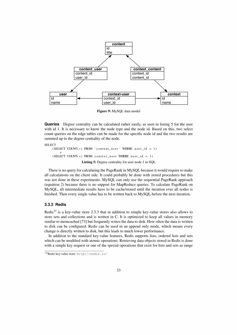
idname

user

idtitle

content

idname

context

context_idcontent_id

context_content

context_iduser_id

context-user

content_iduser_id

content_user

Figure 9: MySQL data model

Queries Degree centrality can be calculated rather easily, as seen in listing 5 for the userwith id 1. It is necessary to know the node type and the node id. Based on this, two selectcount queries on the edge tables can be made for the specific node id and the two results aresummed up to the degree centrality of the node.

SELECT(SELECT COUNT( * ) FROM ‘ c o n t e n t _ u s e r ‘ WHERE u s e r _ i d = 1)

+(SELECT COUNT( * ) FROM c o n t e x t _ u s e r WHERE u s e r _ i d = 1)

Listing 5: Degree centrality for user node 1 in SQL

There is no query for calculating the PageRank in MySQL because it would require to makeall calculations on the client side. It could probably be done with stored procedures but thiswas not done in these experiments. MySQL can only use the sequential PageRank approach(equation 2) because there is no support for MapReduce queries. To calculate PageRank onMySQL, all intermediate results have to be cache/stored until the iteration over all nodes isfinished. Then every single value has to be written back to MySQL before the next iteration.

3.3.2 Redis

Redis33 is a key-value store 2.3.3 that in addition to simple key-value stores also allows tostore sets and collections and is written in C. It is optimized to keep all values in memorysimilar to memcached [73] but frequently writes the data to disk. How often the data is writtento disk can be configured. Redis can be used in an append only mode, which means everychange is directly written to disk, but this leads to much lower performance.

In addition to the standard key-value features, Redis supports lists, ordered lists and setswhich can be modified with atomic operations. Retrieving data objects stored in Redis is donewith a simple key request or one of the special operations that exist for lists and sets as range

33Redis key-value store: http://redis.io/

33

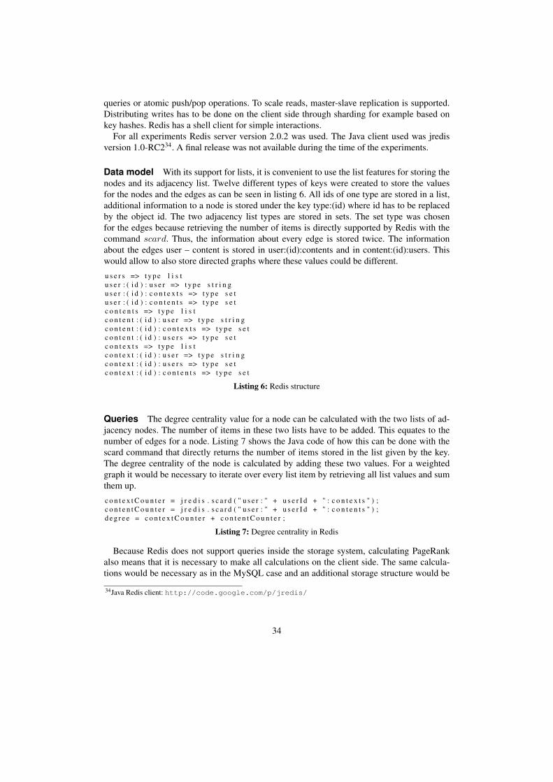
queries or atomic push/pop operations. To scale reads, master-slave replication is supported.Distributing writes has to be done on the client side through sharding for example based onkey hashes. Redis has a shell client for simple interactions.

For all experiments Redis server version 2.0.2 was used. The Java client used was jredisversion 1.0-RC234. A final release was not available during the time of the experiments.

Data model With its support for lists, it is convenient to use the list features for storing thenodes and its adjacency list. Twelve different types of keys were created to store the valuesfor the nodes and the edges as can be seen in listing 6. All ids of one type are stored in a list,additional information to a node is stored under the key type:(id) where id has to be replacedby the object id. The two adjacency list types are stored in sets. The set type was chosenfor the edges because retrieving the number of items is directly supported by Redis with thecommand scard. Thus, the information about every edge is stored twice. The informationabout the edges user – content is stored in user:(id):contents and in content:(id):users. Thiswould allow to also store directed graphs where these values could be different.

u s e r s => t y p e l i s tu s e r : ( i d ) : u s e r => t y p e s t r i n gu s e r : ( i d ) : c o n t e x t s => t y p e s e tu s e r : ( i d ) : c o n t e n t s => t y p e s e tc o n t e n t s => t y p e l i s tc o n t e n t : ( i d ) : u s e r => t y p e s t r i n gc o n t e n t : ( i d ) : c o n t e x t s => t y p e s e tc o n t e n t : ( i d ) : u s e r s => t y p e s e tc o n t e x t s => t y p e l i s tc o n t e x t : ( i d ) : u s e r => t y p e s t r i n gc o n t e x t : ( i d ) : u s e r s => t y p e s e tc o n t e x t : ( i d ) : c o n t e n t s => t y p e s e t

Listing 6: Redis structure

Queries The degree centrality value for a node can be calculated with the two lists of ad-jacency nodes. The number of items in these two lists have to be added. This equates to thenumber of edges for a node. Listing 7 shows the Java code of how this can be done with thescard command that directly returns the number of items stored in the list given by the key.The degree centrality of the node is calculated by adding these two values. For a weightedgraph it would be necessary to iterate over every list item by retrieving all list values and sumthem up.

c o n t e x t C o u n t e r = j r e d i s . s c a r d ( " u s e r : " + u s e r I d + " : c o n t e x t s " ) ;c o n t e n t C o u n t e r = j r e d i s . s c a r d ( " u s e r : " + u s e r I d + " : c o n t e n t s " ) ;d e g r e e = c o n t e x t C o u n t e r + c o n t e n t C o u n t e r ;

Listing 7: Degree centrality in Redis

Because Redis does not support queries inside the storage system, calculating PageRankalso means that it is necessary to make all calculations on the client side. The same calcula-tions would be necessary as in the MySQL case and an additional storage structure would be

34Java Redis client: http://code.google.com/p/jredis/

34

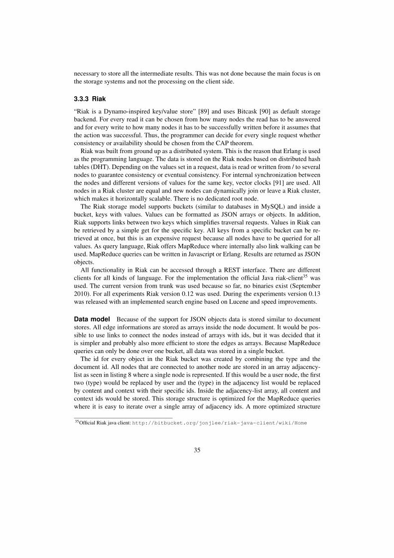
necessary to store all the intermediate results. This was not done because the main focus is onthe storage systems and not the processing on the client side.

3.3.3 Riak

“Riak is a Dynamo-inspired key/value store” [89] and uses Bitcask [90] as default storagebackend. For every read it can be chosen from how many nodes the read has to be answeredand for every write to how many nodes it has to be successfully written before it assumes thatthe action was successful. Thus, the programmer can decide for every single request whetherconsistency or availability should be chosen from the CAP theorem.

Riak was built from ground up as a distributed system. This is the reason that Erlang is usedas the programming language. The data is stored on the Riak nodes based on distributed hashtables (DHT). Depending on the values set in a request, data is read or written from / to severalnodes to guarantee consistency or eventual consistency. For internal synchronization betweenthe nodes and different versions of values for the same key, vector clocks [91] are used. Allnodes in a Riak cluster are equal and new nodes can dynamically join or leave a Riak cluster,which makes it horizontally scalable. There is no dedicated root node.

The Riak storage model supports buckets (similar to databases in MySQL) and inside abucket, keys with values. Values can be formatted as JSON arrays or objects. In addition,Riak supports links between two keys which simplifies traversal requests. Values in Riak canbe retrieved by a simple get for the specific key. All keys from a specific bucket can be re-trieved at once, but this is an expensive request because all nodes have to be queried for allvalues. As query language, Riak offers MapReduce where internally also link walking can beused. MapReduce queries can be written in Javascript or Erlang. Results are returned as JSONobjects.

All functionality in Riak can be accessed through a REST interface. There are differentclients for all kinds of language. For the implementation the official Java riak-client35 wasused. The current version from trunk was used because so far, no binaries exist (September2010). For all experiments Riak version 0.12 was used. During the experiments version 0.13was released with an implemented search engine based on Lucene and speed improvements.

Data model Because of the support for JSON objects data is stored similar to documentstores. All edge informations are stored as arrays inside the node document. It would be pos-sible to use links to connect the nodes instead of arrays with ids, but it was decided that itis simpler and probably also more efficient to store the edges as arrays. Because MapReducequeries can only be done over one bucket, all data was stored in a single bucket.

The id for every object in the Riak bucket was created by combining the type and thedocument id. All nodes that are connected to another node are stored in an array adjacency-list as seen in listing 8 where a single node is represented. If this would be a user node, the firsttwo (type) would be replaced by user and the (type) in the adjacency list would be replacedby content and context with their specific ids. Inside the adjacency-list array, all content andcontext ids would be stored. This storage structure is optimized for the MapReduce querieswhere it is easy to iterate over a single array of adjacency ids. A more optimized structure

35Official Riak java client: http://bitbucket.org/jonjlee/riak-java-client/wiki/Home

35

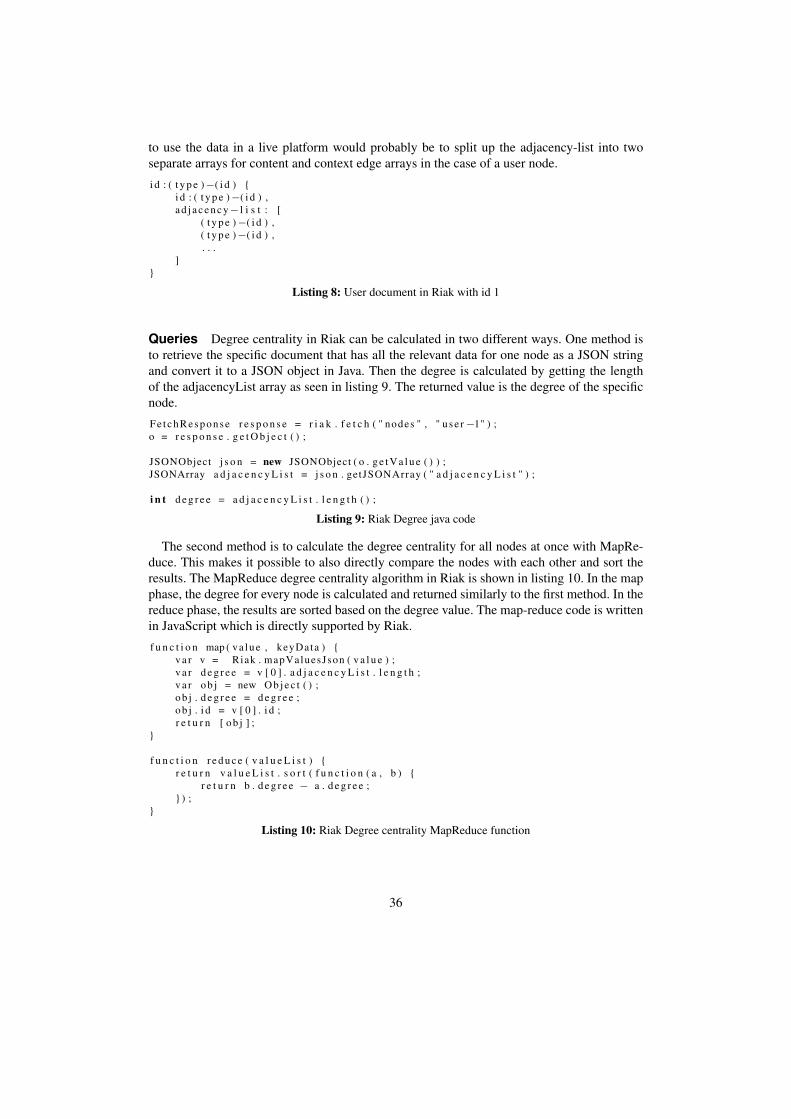
to use the data in a live platform would probably be to split up the adjacency-list into twoseparate arrays for content and context edge arrays in the case of a user node.

i d : ( t y p e ) −( i d ) {i d : ( t y p e ) −( i d ) ,a d j a c e n c y − l i s t : [

( t y p e ) −( i d ) ,( t y p e ) −( i d ) ,. . .

]}

Listing 8: User document in Riak with id 1

Queries Degree centrality in Riak can be calculated in two different ways. One method isto retrieve the specific document that has all the relevant data for one node as a JSON stringand convert it to a JSON object in Java. Then the degree is calculated by getting the lengthof the adjacencyList array as seen in listing 9. The returned value is the degree of the specificnode.

Fe t chResponse r e s p o n s e = r i a k . f e t c h ( " nodes " , " use r −1" ) ;o = r e s p o n s e . g e t O b j e c t ( ) ;

JSONObject j s o n = new JSONObject ( o . g e t V a l u e ( ) ) ;JSONArray a d j a c e n c y L i s t = j s o n . getJSONArray ( " a d j a c e n c y L i s t " ) ;

i n t d e g r e e = a d j a c e n c y L i s t . l e n g t h ( ) ;

Listing 9: Riak Degree java code

The second method is to calculate the degree centrality for all nodes at once with MapRe-duce. This makes it possible to also directly compare the nodes with each other and sort theresults. The MapReduce degree centrality algorithm in Riak is shown in listing 10. In the mapphase, the degree for every node is calculated and returned similarly to the first method. In thereduce phase, the results are sorted based on the degree value. The map-reduce code is writtenin JavaScript which is directly supported by Riak.

f u n c t i o n map ( va lue , keyData ) {v a r v = Riak . mapValuesJson ( v a l u e ) ;v a r d e g r e e = v [ 0 ] . a d j a c e n c y L i s t . l e n g t h ;v a r o b j = new O b j e c t ( ) ;o b j . d e g r e e = d e g r e e ;o b j . i d = v [ 0 ] . i d ;r e t u r n [ o b j ] ;

}

f u n c t i o n r e d u c e ( v a l u e L i s t ) {r e t u r n v a l u e L i s t . s o r t ( f u n c t i o n ( a , b ) {

r e t u r n b . d e g r e e − a . d e g r e e ;} ) ;

}

Listing 10: Riak Degree centrality MapReduce function

36

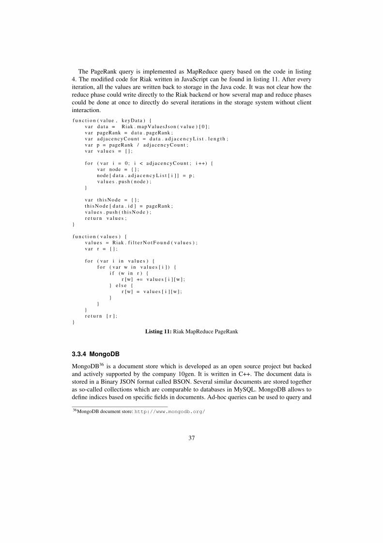
The PageRank query is implemented as MapReduce query based on the code in listing4. The modified code for Riak written in JavaScript can be found in listing 11. After everyiteration, all the values are written back to storage in the Java code. It was not clear how thereduce phase could write directly to the Riak backend or how several map and reduce phasescould be done at once to directly do several iterations in the storage system without clientinteraction.

f u n c t i o n ( va lue , keyData ) {v a r d a t a = Riak . mapValuesJson ( v a l u e ) [ 0 ] ;v a r pageRank = d a t a . pageRank ;v a r a d j a c e n c y C o u n t = d a t a . a d j a c e n c y L i s t . l e n g t h ;v a r p = pageRank / a d j a c e n c y C o u n t ;v a r v a l u e s = [ ] ;

f o r ( v a r i = 0 ; i < a d j a c e n c y C o u n t ; i ++) {v a r node = { } ;node [ d a t a . a d j a c e n c y L i s t [ i ] ] = p ;v a l u e s . push ( node ) ;

}

v a r t h i s N o d e = { } ;t h i s N o d e [ d a t a . i d ] = pageRank ;v a l u e s . push ( t h i s N o d e ) ;r e t u r n v a l u e s ;

}

f u n c t i o n ( v a l u e s ) {v a l u e s = Riak . f i l t e r N o t F o u n d ( v a l u e s ) ;v a r r = { } ;

f o r ( v a r i i n v a l u e s ) {f o r ( v a r w i n v a l u e s [ i ] ) {

i f (w i n r ) {r [w] += v a l u e s [ i ] [w ] ;

} e l s e {r [w] = v a l u e s [ i ] [w ] ;

}}

}r e t u r n [ r ] ;

}

Listing 11: Riak MapReduce PageRank

3.3.4 MongoDB

MongoDB36 is a document store which is developed as an open source project but backedand actively supported by the company 10gen. It is written in C++. The document data isstored in a Binary JSON format called BSON. Several similar documents are stored togetheras so-called collections which are comparable to databases in MySQL. MongoDB allows todefine indices based on specific fields in documents. Ad-hoc queries can be used to query and

36MongoDB document store: http://www.mongodb.org/

37

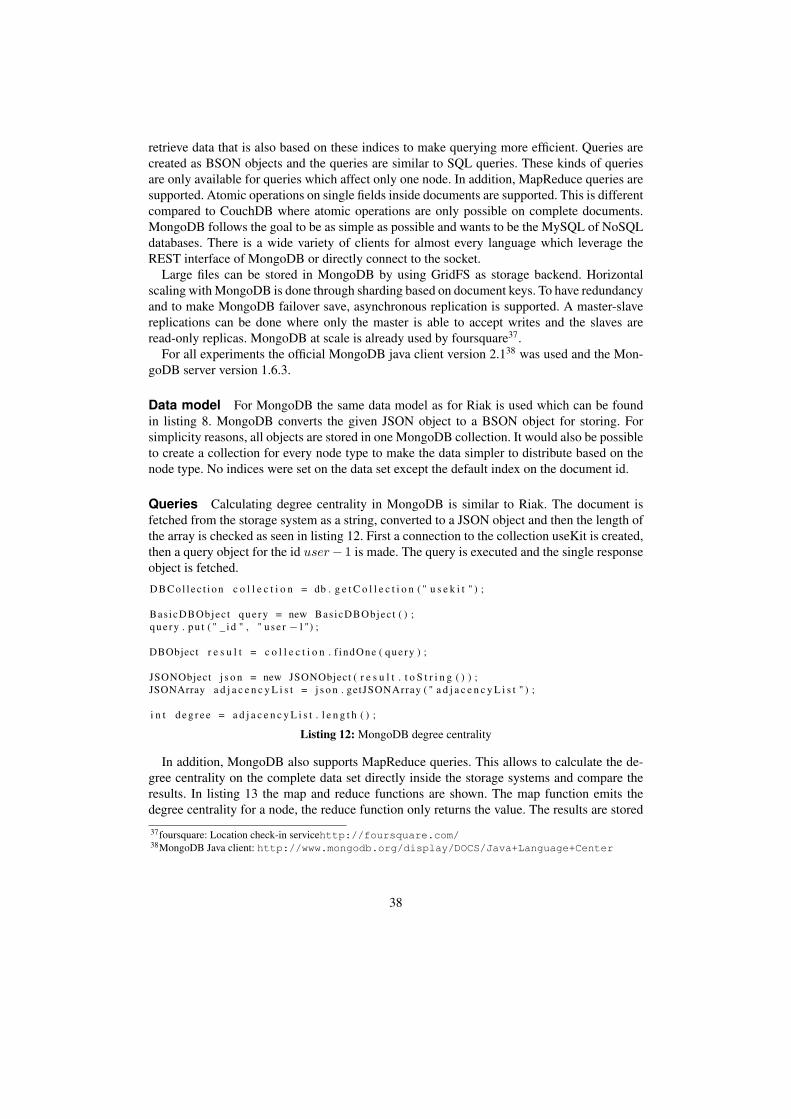
retrieve data that is also based on these indices to make querying more efficient. Queries arecreated as BSON objects and the queries are similar to SQL queries. These kinds of queriesare only available for queries which affect only one node. In addition, MapReduce queries aresupported. Atomic operations on single fields inside documents are supported. This is differentcompared to CouchDB where atomic operations are only possible on complete documents.MongoDB follows the goal to be as simple as possible and wants to be the MySQL of NoSQLdatabases. There is a wide variety of clients for almost every language which leverage theREST interface of MongoDB or directly connect to the socket.

Large files can be stored in MongoDB by using GridFS as storage backend. Horizontalscaling with MongoDB is done through sharding based on document keys. To have redundancyand to make MongoDB failover save, asynchronous replication is supported. A master-slavereplications can be done where only the master is able to accept writes and the slaves areread-only replicas. MongoDB at scale is already used by foursquare37.

For all experiments the official MongoDB java client version 2.138 was used and the Mon-goDB server version 1.6.3.

Data model For MongoDB the same data model as for Riak is used which can be foundin listing 8. MongoDB converts the given JSON object to a BSON object for storing. Forsimplicity reasons, all objects are stored in one MongoDB collection. It would also be possibleto create a collection for every node type to make the data simpler to distribute based on thenode type. No indices were set on the data set except the default index on the document id.

Queries Calculating degree centrality in MongoDB is similar to Riak. The document isfetched from the storage system as a string, converted to a JSON object and then the length ofthe array is checked as seen in listing 12. First a connection to the collection useKit is created,then a query object for the id user− 1 is made. The query is executed and the single responseobject is fetched.

D B C o l l e c t i o n c o l l e c t i o n = db . g e t C o l l e c t i o n ( " u s e k i t " ) ;

Bas icDBObjec t que ry = new BasicDBObjec t ( ) ;que ry . p u t ( " _ i d " , " use r −1") ;

DBObject r e s u l t = c o l l e c t i o n . f indOne ( que ry ) ;

JSONObject j s o n = new JSONObject ( r e s u l t . t o S t r i n g ( ) ) ;JSONArray a d j a c e n c y L i s t = j s o n . getJSONArray ( " a d j a c e n c y L i s t " ) ;

i n t d e g r e e = a d j a c e n c y L i s t . l e n g t h ( ) ;

Listing 12: MongoDB degree centrality

In addition, MongoDB also supports MapReduce queries. This allows to calculate the de-gree centrality on the complete data set directly inside the storage systems and compare theresults. In listing 13 the map and reduce functions are shown. The map function emits thedegree centrality for a node, the reduce function only returns the value. The results are stored

37foursquare: Location check-in servicehttp://foursquare.com/38MongoDB Java client: http://www.mongodb.org/display/DOCS/Java+Language+Center

38

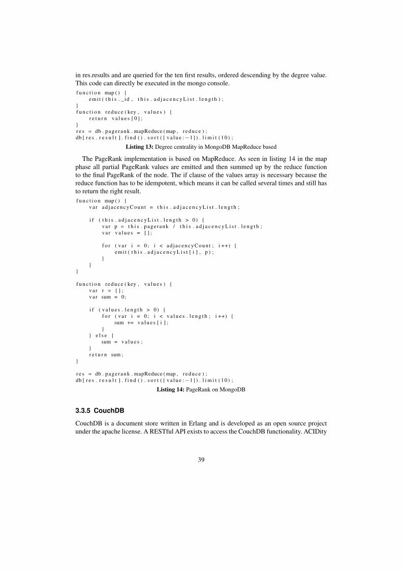
in res.results and are queried for the ten first results, ordered descending by the degree value.This code can directly be executed in the mongo console.f u n c t i o n map ( ) {

emi t ( t h i s . _ id , t h i s . a d j a c e n c y L i s t . l e n g t h ) ;}f u n c t i o n r e d u c e ( key , v a l u e s ) {

r e t u r n v a l u e s [ 0 ] ;}r e s = db . p a g e r a n k . mapReduce ( map , r e d u c e ) ;db [ r e s . r e s u l t ] . f i n d ( ) . s o r t ( { v a l u e : −1}) . l i m i t ( 1 0 ) ;

Listing 13: Degree centrality in MongoDB MapReduce based

The PageRank implementation is based on MapReduce. As seen in listing 14 in the mapphase all partial PageRank values are emitted and then summed up by the reduce functionto the final PageRank of the node. The if clause of the values array is necessary because thereduce function has to be idempotent, which means it can be called several times and still hasto return the right result.f u n c t i o n map ( ) {

v a r a d j a c e n c y C o u n t = t h i s . a d j a c e n c y L i s t . l e n g t h ;

i f ( t h i s . a d j a c e n c y L i s t . l e n g t h > 0) {v a r p = t h i s . p a g e r a n k / t h i s . a d j a c e n c y L i s t . l e n g t h ;v a r v a l u e s = [ ] ;

f o r ( v a r i = 0 ; i < a d j a c e n c y C o u n t ; i ++) {emi t ( t h i s . a d j a c e n c y L i s t [ i ] , p ) ;

}}

}

f u n c t i o n r e d u c e ( key , v a l u e s ) {v a r r = { } ;v a r sum = 0 ;

i f ( v a l u e s . l e n g t h > 0) {f o r ( v a r i = 0 ; i < v a l u e s . l e n g t h ; i ++) {

sum += v a l u e s [ i ] ;}

} e l s e {sum = v a l u e s ;

}r e t u r n sum ;

}

r e s = db . p a g e r a n k . mapReduce ( map , r e d u c e ) ;db [ r e s . r e s u l t ] . f i n d ( ) . s o r t ( { v a l u e : −1}) . l i m i t ( 1 0 ) ;

Listing 14: PageRank on MongoDB

3.3.5 CouchDB

CouchDB is a document store written in Erlang and is developed as an open source projectunder the apache license. A RESTful API exists to access the CouchDB functionality. ACIDity

39

is provided on a document level. CouchDB uses Multi-Version Concurrency Control (MVCC)instead of locks to manage concurrent access to the database and documents. This meansthat every document in CouchDB is versioned. Conflicts can be resolved automatically by thedatabase. The database file on disk is always in a consistent state.

To query data, CouchDB offers so-called views. There are two types of views: Temporaryviews which are only loaded into memory and permanent views that are stored on disk andloaded into the system on startup. Views are MapReduce functions written in JavaScript thatprocess the stored data and return the results. A query language similar to SQL is not sup-ported. Indices on specific fields are not supported but indices are automatically created forthe view results. The results of views are only once completely calculated and then updatedevery time data is added or updated in the system, which makes the views much more effi-cient. The generated views can also be distributed to several CouchDB nodes, which makesit possible to distribute queries. Since version 0.11 CouchDB supports linking documents inview queries.

Scaling reads in CouchDB is done through asynchronous incremental replication. For writesCouchDB started to support sharding of data as it is already provided by the CouchDB Loungeextension, but this is still under development. Partitioning data should be supported in thefuture.

CouchDB is already used in research for Data Management and Workflow Management atCERN, the European Organization for Nuclear Research[92]. As CouchDB client couchdb4j39

for Java was used. Because there were no up-to-date releases, the current version from trunkwas used. Other Java clients that were evaluated were ektorp40 and jrelax41. The decision wasmade for couchdb4j because of its simplicity.

Data model The useKit data for CouchDB was modeled in the exact same way as forMongoDB and Riak, which can be found in listing 8. CouchDB directly stores the data inJSON format, similarly to Riak.

Query The degree centrality in CouchDB is calculated with a MapReduce query that createsa view. Based on this view, CouchDB creates indices to query the data more efficiently. Toretrieve the top ten nodes based on the degree centrality, the query in listing 15 is used. Noreduce function is needed because the results are already sorted by the return key which is thedegree with the document id as value.

f u n c t i o n ( doc ) {emi t ( doc . a d j a c e n c y L i s t . l e n g t h , doc . i d ) ;

}

Listing 15: Degree centrality in Riak

The PageRank MapReduce query did not work on CouchDB. The CouchDB MapReducequeries require a specific reduce factor in the reduce phase. The number of results after thefirst reduce step has to be significantly smaller than in the map phase. This factor is predefined

39CouchDB Java client from Marcus Breese: http://github.com/mbreese/couchdb4j40Ektorp CouchDB Java client: http://code.google.com/p/ektorp/41jrelax CouchDB Java client: http://wiki.github.com/isterin/jrelax/

40

by the CouchDB query system and throws an error if the number of results in the reduce phasedoes not reduce fast enough. As in the PageRank algorithm, the number of start nodes beforethe map phase and after the reduce phase are both the total number of nodes and are thusexactly the same. The PageRank query in CouchDB always threw an error because the reducefactor was not large enough, which made it impossible to implement the PageRank algorithmin CouchDB. No configuration parameter was found to disable this check.

3.3.6 HBase

HBase [93] is a column storage based on the Hadoop Distributed File System (HDFS)42 cre-ated with the idea of BigTable [59] in mind. The HBase project is open source. HBase isstrongly consistent and picks consistency and partition tolerance from the CAP theorem asseen in figure 4. HBase is like Hadoop completely written in Java43. To access HBase, theThrift[64] interface is used, but also REST calls are supported. Indices are automatically cre-ated for all row keys and are sorted lexicographically. Internally, B-Trees are used for indicesbased on which sorting and range queries are made. HBase supports transactional calls withstrong consistency in comparison to Cassandra which is based on MVCC. Still, HBase sup-ports versioning and conflict resolution.

The HBase data model is based on the BigTable data model as seen in figure 5. A tablecontains rows where every row is an array of bytes. HBase keeps rows lexicographically or-dered. Every row can have several column families which are the same for every row in a table.Every column family can have several column keys with values inside. To retrieve a specificvalue, the row key, column family, column key and the timestamp have to be known. If thetimestamp is left out, the newest version of the value is returned. HBase stores a timestamp inmilliseconds with every value.

HBase supports range queries or can be used as key-value stores where the key has to beknown to fetch the data. For data processing and more complex queries of the complete dataset, MapReduce queries are supported, which are executed in Hadoop.

Scaling HBase can be done by distributing the data to several nodes. HBase clusters have aso-called name node which manages the task and data distribution. There can be a single pointof failure if the name node is not redundant. Managing and coordinating HBase data and namenodes is often done with Zookeeper44, a high-performance coordination service. If HBase isused in combination with Hadoop for the data processing of an additional node, a so-calledtasktracker is necessary to distribute tasks to the clients. More detailed information about theperformance of HBase can be found in the paper of Carstoiu et al [94]. Replication in HBaseis done based on log files.

HBase in combination with Hadoop for data processing is used by several companies suchas Twitter, Facebook or Yahoo in large scale, which means more than 1000 nodes. The com-pany cloudera offers Hadoop in combination with HBase for enterprises. They also offer sim-ple packages for linux that can be installed with the package manager which makes setting upHBase much simpler.

42Hadoop Distributed File System: http://hadoop.apache.org/hdfs/43HBase Java API http://hbase.apache.org/docs/current/api/overview-summary.html44Zookeeper: Centralized managing service: http://hadoop.apache.org/zookeeper/

41

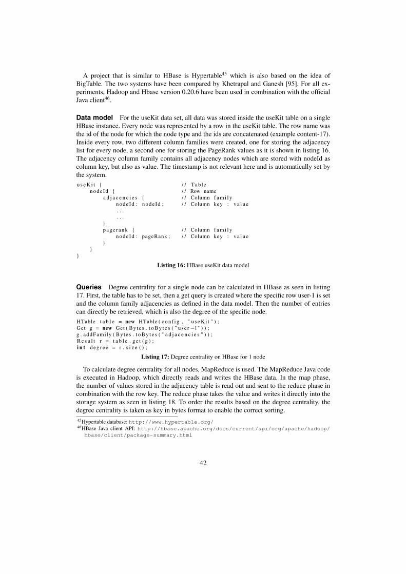
A project that is similar to HBase is Hypertable45 which is also based on the idea ofBigTable. The two systems have been compared by Khetrapal and Ganesh [95]. For all ex-periments, Hadoop and Hbase version 0.20.6 have been used in combination with the officialJava client46.

Data model For the useKit data set, all data was stored inside the useKit table on a singleHBase instance. Every node was represented by a row in the useKit table. The row name wasthe id of the node for which the node type and the ids are concatenated (example content-17).Inside every row, two different column families were created, one for storing the adjacencylist for every node, a second one for storing the PageRank values as it is shown in listing 16.The adjacency column family contains all adjacency nodes which are stored with nodeId ascolumn key, but also as value. The timestamp is not relevant here and is automatically set bythe system.u s e K i t { / / Tab le

nodeId { / / Row namea d j a c e n c i e s { / / Column f a m i l y

nodeId : nodeId ; / / Column key : v a l u e. . .. . .

}p a g e r a n k { / / Column f a m i l y

nodeId : pageRank ; / / Column key : v a l u e}

}}

Listing 16: HBase useKit data model

Queries Degree centrality for a single node can be calculated in HBase as seen in listing17. First, the table has to be set, then a get query is created where the specific row user-1 is setand the column family adjacencies as defined in the data model. Then the number of entriescan directly be retrieved, which is also the degree of the specific node.HTable t a b l e = new HTable ( c o n f i g , " u s e K i t " ) ;Get g = new Get ( By tes . t o B y t e s ( " use r −1" ) ) ;g . addFami ly ( By tes . t o B y t e s ( " a d j a c e n c i e s " ) ) ;R e s u l t r = t a b l e . g e t ( g ) ;i n t d e g r e e = r . s i z e ( ) ;

Listing 17: Degree centrality on HBase for 1 node

To calculate degree centrality for all nodes, MapReduce is used. The MapReduce Java codeis executed in Hadoop, which directly reads and writes the HBase data. In the map phase,the number of values stored in the adjacency table is read out and sent to the reduce phase incombination with the row key. The reduce phase takes the value and writes it directly into thestorage system as seen in listing 18. To order the results based on the degree centrality, thedegree centrality is taken as key in bytes format to enable the correct sorting.45Hypertable database: http://www.hypertable.org/46HBase Java client API: http://hbase.apache.org/docs/current/api/org/apache/hadoop/

hbase/client/package-summary.html

42

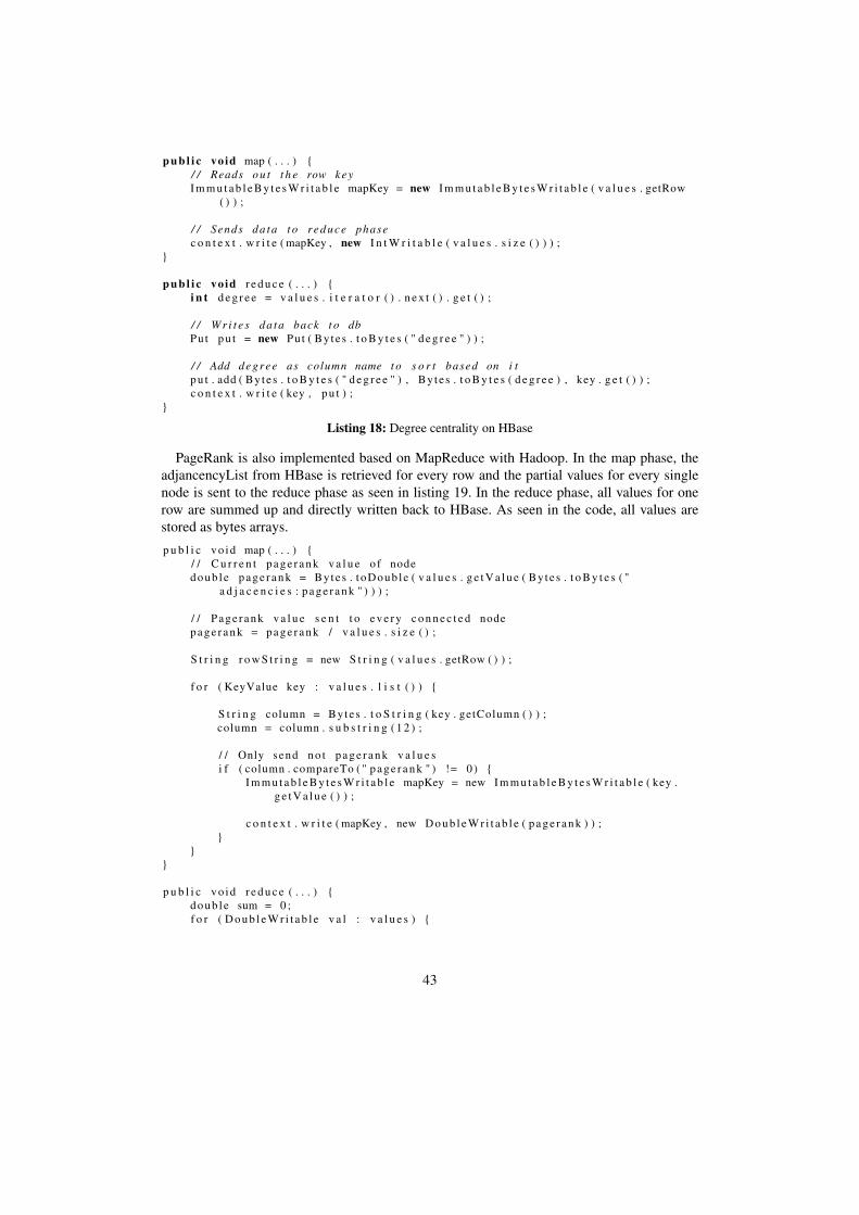
p u b l i c vo id map ( . . . ) {/ / Reads o u t t h e row keyI m m u t a b l e B y t e s W r i t a b l e mapKey = new I m m u t a b l e B y t e s W r i t a b l e ( v a l u e s . getRow

( ) ) ;

/ / Sends da ta t o r ed uc e phasec o n t e x t . w r i t e ( mapKey , new I n t W r i t a b l e ( v a l u e s . s i z e ( ) ) ) ;

}

p u b l i c vo id r e d u c e ( . . . ) {i n t d e g r e e = v a l u e s . i t e r a t o r ( ) . n e x t ( ) . g e t ( ) ;

/ / W r i t e s da ta back t o dbPut p u t = new Put ( By tes . t o B y t e s ( " d e g r e e " ) ) ;

/ / Add de g re e as column name t o s o r t based on i tp u t . add ( By tes . t o B y t e s ( " d e g r e e " ) , By tes . t o B y t e s ( d e g r e e ) , key . g e t ( ) ) ;c o n t e x t . w r i t e ( key , p u t ) ;

}

Listing 18: Degree centrality on HBase

PageRank is also implemented based on MapReduce with Hadoop. In the map phase, theadjancencyList from HBase is retrieved for every row and the partial values for every singlenode is sent to the reduce phase as seen in listing 19. In the reduce phase, all values for onerow are summed up and directly written back to HBase. As seen in the code, all values arestored as bytes arrays.

p u b l i c vo id map ( . . . ) {/ / C u r r e n t p a g e r a n k v a l u e o f nodedo ub l e p a g e r a n k = Bytes . toDoub le ( v a l u e s . g e t V a l u e ( By tes . t o B y t e s ( "

a d j a c e n c i e s : p a g e r a n k " ) ) ) ;

/ / Page rank v a l u e s e n t t o e v e r y c o n n e c t e d nodep a g e r a n k = p a g e r a n k / v a l u e s . s i z e ( ) ;

S t r i n g r o w S t r i n g = new S t r i n g ( v a l u e s . getRow ( ) ) ;

f o r ( KeyValue key : v a l u e s . l i s t ( ) ) {

S t r i n g column = Bytes . t o S t r i n g ( key . getColumn ( ) ) ;column = column . s u b s t r i n g ( 1 2 ) ;

/ / Only send n o t p a g e r a n k v a l u e si f ( column . compareTo ( " p a g e r a n k " ) != 0 ) {

I m m u t a b l e B y t e s W r i t a b l e mapKey = new I m m u t a b l e B y t e s W r i t a b l e ( key .g e t V a l u e ( ) ) ;

c o n t e x t . w r i t e ( mapKey , new D o u b l e W r i t a b l e ( p a g e r a n k ) ) ;}

}}

p u b l i c vo id r e d u c e ( . . . ) {do ub l e sum = 0 ;f o r ( D o u b l e W r i t a b l e v a l : v a l u e s ) {

43

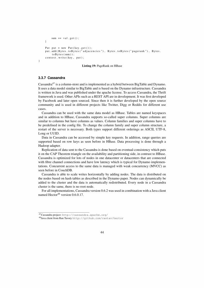
sum += v a l . g e t ( ) ;}

Pu t p u t = new Put ( key . g e t ( ) ) ;p u t . add ( By tes . t o B y t e s ( " a d j a c e n c i e s " ) , By tes . t o B y t e s ( " p a g e r a n k " ) , By te s .

t o B y t e s ( sum ) ) ;c o n t e x t . w r i t e ( key , p u t ) ;

}

Listing 19: PageRank on HBase

3.3.7 Cassandra

Cassandra47 is a column-store and is implemented as a hybrid between BigTable and Dynamo.It uses a data model similar to BigTable and is based on the Dynamo infrastructure. Cassandrais written in Java and was published under the apache license. To access Cassandra, the Thriftframework is used. Other APIs such as a REST API are in development. It was first developedby Facebook and later open sourced. Since then it is further developed by the open sourcecommunity and is used in different projects like Twitter, Digg or Reddis for different usecases.

Cassandra can be used with the same data model as HBase. Tables are named keyspacesand in addition to HBase, Cassandra supports so-called super columns. Super columns aresimilar to columns but have columns as values. Column families and super columns have tobe predefined in the config file. To change the column family and super column structure, arestart of the server is necessary. Both types support different orderings as ASCII, UTF-8,Long or UUID.

Data in Cassandra can be accessed by simple key requests. In addition, range queries aresupported based on row keys as seen before in HBase. Data processing is done through aHadoop adapter.

Replication of data sent to the Cassandra is done based on eventual-consistency which putsit on the CAP Theorem triangle on the availability and partitioning side, in contrast to HBase.Cassandra is optimized for lots of nodes in one datacenter or datacenters that are connectedwith fibre channel connections and have low latency which is typical for Dynamo implemen-tations. Concurrent access to the same data is managed with weak concurrency (MVCC) asseen before in CouchDB.

Cassandra is able to scale writes horizontally by adding nodes. The data is distributed onthe nodes based on hash tables as described in the Dynamo paper. Nodes can dynamically beadded to the cluster and the data is automatically redistributed. Every node in a Cassandracluster is the same, there is no root node.

For all implementations, Cassandra version 0.6.2 was used in combination with a Java clientnamed Hector48 version 0.6.0.17.

47Cassandra project: http://cassandra.apache.org/48Java client from Ran Tavory http://github.com/rantav/hector

44

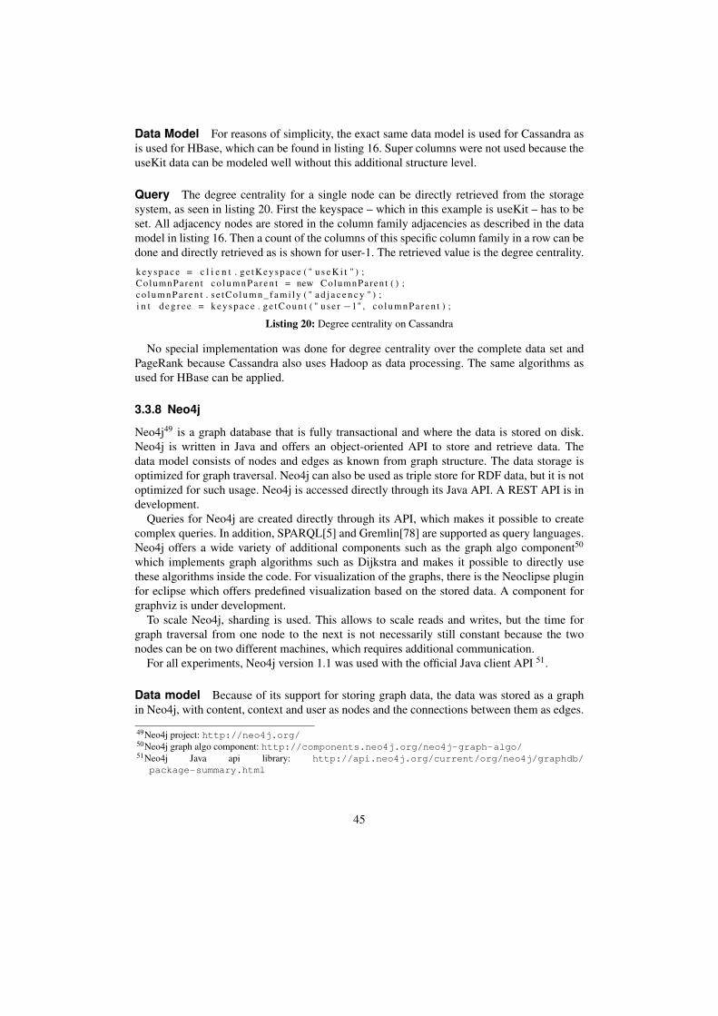
Data Model For reasons of simplicity, the exact same data model is used for Cassandra asis used for HBase, which can be found in listing 16. Super columns were not used because theuseKit data can be modeled well without this additional structure level.

Query The degree centrality for a single node can be directly retrieved from the storagesystem, as seen in listing 20. First the keyspace – which in this example is useKit – has to beset. All adjacency nodes are stored in the column family adjacencies as described in the datamodel in listing 16. Then a count of the columns of this specific column family in a row can bedone and directly retrieved as is shown for user-1. The retrieved value is the degree centrality.

k e y s p a c e = c l i e n t . ge tKeyspace ( " u s e K i t " ) ;ColumnParent c o l u m n P a r e n t = new ColumnParent ( ) ;c o l u m n P a r e n t . s e t C o l u m n _ f a m i l y ( " a d j a c e n c y " ) ;i n t d e g r e e = k e y s p a c e . g e t C ou n t ( " use r −1" , c o l u m n P a r e n t ) ;

Listing 20: Degree centrality on Cassandra

No special implementation was done for degree centrality over the complete data set andPageRank because Cassandra also uses Hadoop as data processing. The same algorithms asused for HBase can be applied.

3.3.8 Neo4j

Neo4j49 is a graph database that is fully transactional and where the data is stored on disk.Neo4j is written in Java and offers an object-oriented API to store and retrieve data. Thedata model consists of nodes and edges as known from graph structure. The data storage isoptimized for graph traversal. Neo4j can also be used as triple store for RDF data, but it is notoptimized for such usage. Neo4j is accessed directly through its Java API. A REST API is indevelopment.

Queries for Neo4j are created directly through its API, which makes it possible to createcomplex queries. In addition, SPARQL[5] and Gremlin[78] are supported as query languages.Neo4j offers a wide variety of additional components such as the graph algo component50

which implements graph algorithms such as Dijkstra and makes it possible to directly usethese algorithms inside the code. For visualization of the graphs, there is the Neoclipse pluginfor eclipse which offers predefined visualization based on the stored data. A component forgraphviz is under development.

To scale Neo4j, sharding is used. This allows to scale reads and writes, but the time forgraph traversal from one node to the next is not necessarily still constant because the twonodes can be on two different machines, which requires additional communication.

For all experiments, Neo4j version 1.1 was used with the official Java client API 51.

Data model Because of its support for storing graph data, the data was stored as a graphin Neo4j, with content, context and user as nodes and the connections between them as edges.

49Neo4j project: http://neo4j.org/50Neo4j graph algo component: http://components.neo4j.org/neo4j-graph-algo/51Neo4j Java api library: http://api.neo4j.org/current/org/neo4j/graphdb/

package-summary.html

45

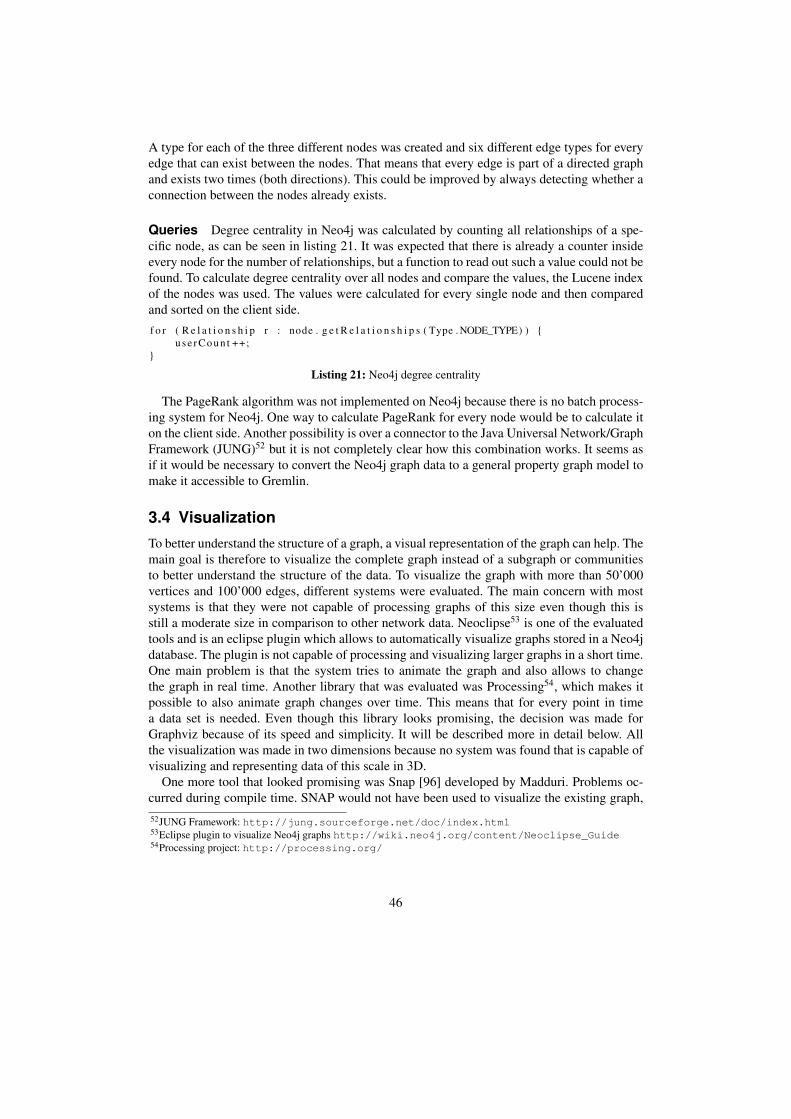
A type for each of the three different nodes was created and six different edge types for everyedge that can exist between the nodes. That means that every edge is part of a directed graphand exists two times (both directions). This could be improved by always detecting whether aconnection between the nodes already exists.

Queries Degree centrality in Neo4j was calculated by counting all relationships of a spe-cific node, as can be seen in listing 21. It was expected that there is already a counter insideevery node for the number of relationships, but a function to read out such a value could not befound. To calculate degree centrality over all nodes and compare the values, the Lucene indexof the nodes was used. The values were calculated for every single node and then comparedand sorted on the client side.

f o r ( R e l a t i o n s h i p r : node . g e t R e l a t i o n s h i p s ( Type . NODE_TYPE) ) {u s e r C o u n t ++;

}

Listing 21: Neo4j degree centrality

The PageRank algorithm was not implemented on Neo4j because there is no batch process-ing system for Neo4j. One way to calculate PageRank for every node would be to calculate iton the client side. Another possibility is over a connector to the Java Universal Network/GraphFramework (JUNG)52 but it is not completely clear how this combination works. It seems asif it would be necessary to convert the Neo4j graph data to a general property graph model tomake it accessible to Gremlin.

3.4 VisualizationTo better understand the structure of a graph, a visual representation of the graph can help. Themain goal is therefore to visualize the complete graph instead of a subgraph or communitiesto better understand the structure of the data. To visualize the graph with more than 50’000vertices and 100’000 edges, different systems were evaluated. The main concern with mostsystems is that they were not capable of processing graphs of this size even though this isstill a moderate size in comparison to other network data. Neoclipse53 is one of the evaluatedtools and is an eclipse plugin which allows to automatically visualize graphs stored in a Neo4jdatabase. The plugin is not capable of processing and visualizing larger graphs in a short time.One main problem is that the system tries to animate the graph and also allows to changethe graph in real time. Another library that was evaluated was Processing54, which makes itpossible to also animate graph changes over time. This means that for every point in timea data set is needed. Even though this library looks promising, the decision was made forGraphviz because of its speed and simplicity. It will be described more in detail below. Allthe visualization was made in two dimensions because no system was found that is capable ofvisualizing and representing data of this scale in 3D.

One more tool that looked promising was Snap [96] developed by Madduri. Problems oc-curred during compile time. SNAP would not have been used to visualize the existing graph,52JUNG Framework: http://jung.sourceforge.net/doc/index.html53Eclipse plugin to visualize Neo4j graphs http://wiki.neo4j.org/content/Neoclipse_Guide54Processing project: http://processing.org/

46

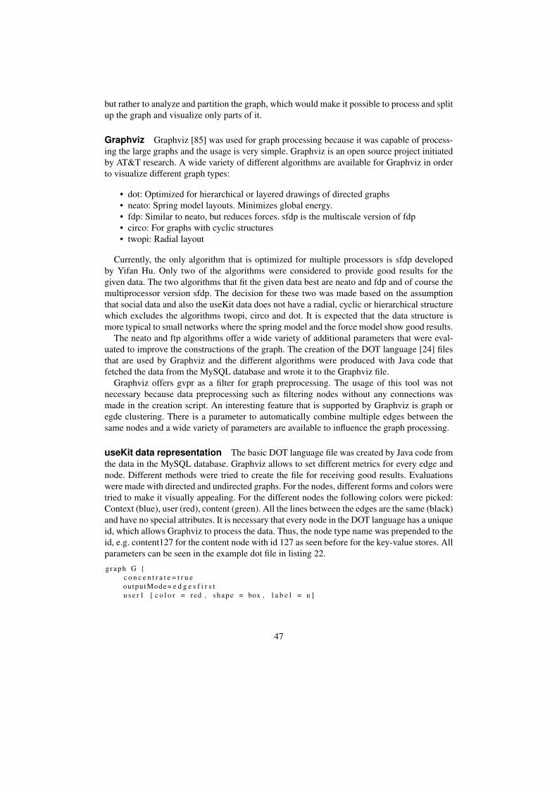
but rather to analyze and partition the graph, which would make it possible to process and splitup the graph and visualize only parts of it.

Graphviz Graphviz [85] was used for graph processing because it was capable of process-ing the large graphs and the usage is very simple. Graphviz is an open source project initiatedby AT&T research. A wide variety of different algorithms are available for Graphviz in orderto visualize different graph types:

• dot: Optimized for hierarchical or layered drawings of directed graphs• neato: Spring model layouts. Minimizes global energy.• fdp: Similar to neato, but reduces forces. sfdp is the multiscale version of fdp• circo: For graphs with cyclic structures• twopi: Radial layout

Currently, the only algorithm that is optimized for multiple processors is sfdp developedby Yifan Hu. Only two of the algorithms were considered to provide good results for thegiven data. The two algorithms that fit the given data best are neato and fdp and of course themultiprocessor version sfdp. The decision for these two was made based on the assumptionthat social data and also the useKit data does not have a radial, cyclic or hierarchical structurewhich excludes the algorithms twopi, circo and dot. It is expected that the data structure ismore typical to small networks where the spring model and the force model show good results.

The neato and ftp algorithms offer a wide variety of additional parameters that were eval-uated to improve the constructions of the graph. The creation of the DOT language [24] filesthat are used by Graphviz and the different algorithms were produced with Java code thatfetched the data from the MySQL database and wrote it to the Graphviz file.

Graphviz offers gvpr as a filter for graph preprocessing. The usage of this tool was notnecessary because data preprocessing such as filtering nodes without any connections wasmade in the creation script. An interesting feature that is supported by Graphviz is graph oregde clustering. There is a parameter to automatically combine multiple edges between thesame nodes and a wide variety of parameters are available to influence the graph processing.

useKit data representation The basic DOT language file was created by Java code fromthe data in the MySQL database. Graphviz allows to set different metrics for every edge andnode. Different methods were tried to create the file for receiving good results. Evaluationswere made with directed and undirected graphs. For the nodes, different forms and colors weretried to make it visually appealing. For the different nodes the following colors were picked:Context (blue), user (red), content (green). All the lines between the edges are the same (black)and have no special attributes. It is necessary that every node in the DOT language has a uniqueid, which allows Graphviz to process the data. Thus, the node type name was prepended to theid, e.g. content127 for the content node with id 127 as seen before for the key-value stores. Allparameters can be seen in the example dot file in listing 22.

graph G {c o n c e n t r a t e = t r u eoutputMode= e d g e s f i r s tu s e r 1 [ c o l o r = red , shape = box , l a b e l = u ]

47

u s e r 1 −− c o n t e x t 8u s e r 1 −− c o n t e x t 1 1 1u s e r 5 [ c o l o r = red , shape = box , l a b e l = u ]u s e r 5 −− c o n t e x t 1 1 1u s e r 5 −− c o n t e x t 1 6. . .c o n t e x t 1 1 [ c o l o r = blue , l a b e l = c ]c o n t e x t 1 1 −− c o n t e n t 2 3 8. . .c o n t e n t 2 3 8 [ c o l o r = green , shape = p o i n t ]. . .

}

Listing 22: DOT Language file

3.5 Experiment setupAll installations and experiments were made on two different machines. One was a desktopmachine with two Intel Pentium 4 CPU 2.80GHz processors, 2 GB of RAM and a 80GB harddrive. The system was running a default Ubuntu 10.4 server installation. The second machinewas a MacBook Pro with an Intel Core 2 Duo 2.53 GHZ processor, 4 GB of RAM and 500GBhard drive (7200RPM). Hardware with more RAM was not available. For the various storagesystems, the default setup and default configurations were used. For performance comparisonsit would be necessary to configure every system for the specific use case to optimize theperformance. For the file storage systems the max number of allowed open files and allowedprocesses was increased because most storage systems use a large number of open files atthe same time. More details about the setup can be found on the wiki pages created for thisthesis55.

To process large graphs and have access to a larger amount of memory, an extra large EC2instance from Amazon was deployed for a short time. This gave access to faster and a largernumber of CPUs. In collaboration with the math institute at the University of Basel, access toa machine with 16 Intel Xeon 2.67 CPUs and 48GB of memory for fast graph processing waspossible. This significantly reduced the time to visualize graphs. To display and analyze thesvg files produced by Graphviz the ZRGViewer56 was used.

55Thesis documentation with detailed setup: http://ruflin.com/wiki/master-thesis:index56ZGRViewer, a GraphViz/DOT Viewer: http://zvtm.sourceforge.net/zgrviewer.html

48

4 Analysis and ResultsIn this thesis, the structure of social data and social networks was analyzed to compare thedifferent types of social data. The useKit data as an example for social data has been modeled,stored and processed with different storage systems and was analyzed in detail to evaluate howadequate the different storage system are for social data. Every storage system has shown itsadvantages and disadvantages for the different processing methods. To better understand theglobal structure of the useKit data, the data set was visualized with Graphviz.

4.1 Data structureThe data structure of different social networks was analyzed based on the functionalities thatthe social network platforms offer. The useKit data set was analyzed in depth and will bedescribed in detail.

4.1.1 Social data

Analyzing the data structure of different social networks reveals that the network structure isdifferent for every network. The common denominator that can be found for all social data isthat all consist of nodes and edges and can be represented as a graph. Every network can con-sist of different node and edge types. A differentiation between directed and undirected edgeshas to be made. An example of this can be seen by comparing the social graph of Facebookand Twitter where the users in Facebook build a friend graph which is based on friendships andwhere the connections are bidirectional, which means that the users are connected by undi-rected edges. The users in Twitter represent a directed social graph mostly based on interestswhich also leads to a different overall structure. The social graph in useKit is based on smallcollaborative networks and interest networks which again results in a different graph structurewith lots of small clusters which is shown through the visualization of the data in section 4.4.

Social data differs from web link data in its overall structure and in how the graph changesover time. In figure 10 two small social networks with the same nodes but different edgesin between are shown. The social network A consists of two highly connected communitieswhich have few connections in between. The social network B consists of three highly con-nected communities which also have a few connections in between. The change from socialnetwork A to B over time is typical for social networks. The communities change over time,new communities appear, others disappear which means the edges between the nodes change.This is the same in the real world, where new friendships arise and if e.g. a person moves toa different place, some relationships are lost and new communities are joined. This alteringoverall structure of social networks is especially relevant for storage systems. To minimizequeries over several machines, it makes sense to store highly connected communities on thesame machine. But because of the changing communities this cannot be done without redis-tributing the nodes every time a community changes. If for the social network A in figure 10the community on the left would be stored on machine one and the community on the right sidewould be stored on machine two, this would be ideal because there are only few connectionsbetween these nodes, which means little communication is necessary.

49

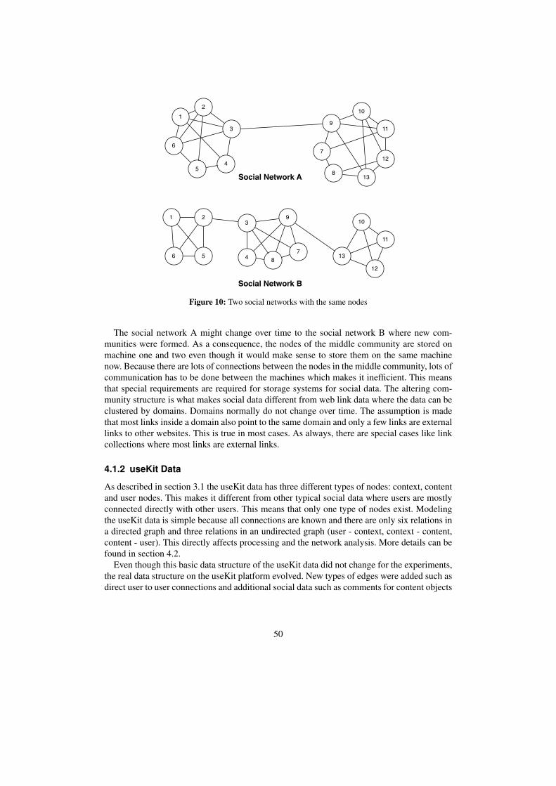
1

6

3

54

2

9

13

10

712

11

8

1

6

3

5 4

2 9

13

10

7

12

11

8

Social Network A

Social Network B

Figure 10: Two social networks with the same nodes

The social network A might change over time to the social network B where new com-munities were formed. As a consequence, the nodes of the middle community are stored onmachine one and two even though it would make sense to store them on the same machinenow. Because there are lots of connections between the nodes in the middle community, lots ofcommunication has to be done between the machines which makes it inefficient. This meansthat special requirements are required for storage systems for social data. The altering com-munity structure is what makes social data different from web link data where the data can beclustered by domains. Domains normally do not change over time. The assumption is madethat most links inside a domain also point to the same domain and only a few links are externallinks to other websites. This is true in most cases. As always, there are special cases like linkcollections where most links are external links.

4.1.2 useKit Data

As described in section 3.1 the useKit data has three different types of nodes: context, contentand user nodes. This makes it different from other typical social data where users are mostlyconnected directly with other users. This means that only one type of nodes exist. Modelingthe useKit data is simple because all connections are known and there are only six relations ina directed graph and three relations in an undirected graph (user - context, context - content,content - user). This directly affects processing and the network analysis. More details can befound in section 4.2.

Even though this basic data structure of the useKit data did not change for the experiments,the real data structure on the useKit platform evolved. New types of edges were added such asdirect user to user connections and additional social data such as comments for content objects

50

were added. It is typical for social data that new features are added frequently to the socialnetworks which change the data structure. Every time the structure changes, new processingmethods have to be evaluated and the existing ones have to be adapted to the new structureand data.

Only the minimal node information was used for all calculations and processing. All addi-tional information that exists for every node – such as first name and last name for the usernodes or context name for the context node – were ignored. This made the data much morecompact for storage and processing.

Prior to the experiments, the structure of the useKit network was mostly unknown. Throughthe processing, analysis and visualization of the useKit data, a better understanding of the dataset was achieved. As can be seen in the visualization section and in figure 13 useKit consistsof many small communities that are highly connected. There are large connected clusterswith highly connected sub-communities inside. There are no nodes that are central for thecomplete network, which means that every community has connections to these nodes. Thiscan be explained by how the useKit platform is used, namely for collaboration in small teams.The content, context and user nodes are highly connected among the teams but only few data isimportant to the outside, which means only a few connections exist outside of the team. Publiccontexts are the only nodes that can attract lots of users and lots of content which would makeit possible that public contexts, like the Music context, could get globally popular.

4.2 Network analysisDifferent centrality measures were calculated on the useKit data to analyze the data set. Thegoal of the analysis was to find central nodes in the system. Only a limited amount of networkanalysis algorithms were used because of time restrictions. All the processing of the datawas done on a snapshot of the data from the beginning of October. Since then, the originaldata set grew. The two well-known centrality measures degree centrality and PageRank werecalculated on the data set. The different algorithms were implement on all storage systems.The results of the calculations were the same on every system as expected even though therewere different methods that were used to receive the results.

4.2.1 Degree centrality

The degree centrality calculation was done for all types of nodes. Because of the different nodetypes it was tried to calculate degree centrality with weighted edges. The reason for this wasthe assumption that a user or a context object are likely to be more important than a contentobject. It is expected that most users are connected to each other over contexts. This meansthat a user with many contexts should have a higher degree than a user with many contents.Comparing the values with weighted edges and without weighted edges, it seemed as if therelative values are quite similar. One explanation for this is that a user with many contents isalso likely to have many contexts to organize their content and the other way around. Thus,degree centrality was only calculated with unweighted edges.

In this thesis, it was assumed that the degree centrality will not describe the central nodesvery well and it will have a lots of false information. The reason for this is that no relationsto other users are necessary to receive a high degree centrality. A user with lots of content

51

items and contexts can have a high degree centrality without being important or central inthe network. But as we see later, the degree centrality values matched the PageRank valuesquite well. This could be explained by the fact that in the useKit network there is nothing togain for the users by having a high degree centrality – in contrast to Google, where it caninfluence the PageRank and thus it can directly influence how often a website is found. Thismeans that there are no users that try to create as many connections to their own profile aspossible. The useKit platform is used to store, retrieve and share data so that all generatedcontent is somehow connected to the user and makes sense for the user. A user with lots ofcontent and context will not gain more power in the useKit network. Instead, if a user createslots of nonsense content, he will probably loose connections to others. The useKit platform isstill in beta stage, which means that most users use the platform in the expected way. As soonas the platform grows this can change and attract also spam bots and other users that try tomisuse the system. This could change the values.

In the top ten results for all nodes were seven user nodes, three context nodes and zerocontent nodes. The top users are users in the system that actively use the system in theireveryday life, which means they create lots of content, create contexts to share the contentand invite other users to collaborate. One of the top ten users was Nicolas Ruflin, the writer ofthis thesis. The degree centrality of this user is high in comparison to other users. This can beexplained by two facts: He was one of the first people that was able to use the system and healso heavily tests the live system.

All three top contexts in the top ten are public contexts. One of these contexts is the context"Master Thesis Nicolas Ruflin" which was used to collect content for this thesis. This contextis in the top ten because of its massive amount of content items. One other public context isthe "Music" context which has – in addition to the other contexts – also lots of users. Thisleads to a high degree centrality value. It makes sense that all contexts with a high degree arepublic contexts. A public context can be joined by everyone, and as long as it is not set to readonly in the system, all users can add content.

There were no content objects in the top 100 results. This can be explained by the fact thatnormally, content objects only belong to one to four contexts and are owned by only a fewusers. If a context has some content objects, the degree of the context is already higher thanthe degree of the content object itself because more connections exist. The main question thatshould be asked here is how an important or central content can be described. There is no realsolution to that with the degree centrality where content objects will always be at the end ofthe rankings if they are not owned by lots of users.

In figure 11 four plots with the degree centrality of the top 50 nodes for every type areshown. In the top left graph the values for the top 50 users are compared. There are a fewusers in the system that have a degree centrality larger than 1000. These are very active users.The degree centrality drops fast and then the average user has a degree centrality of around 50.The same can be seen in respect to contexts. There are a few contexts with a degree larger than100, but the average context has a degree centrality of 28. The peaks for the context objectscan be explained by the power law. If a context is popular, even more users will join it andeven more content will be added. For the content objects the values are much lower because itis rare that a content object belongs to many users or is in many contexts. In the top 50 contentobjects, the objects all have a degree centrality around 6, the overall average is around 3. Onthe right bottom, all graphs are combined into one graph. This makes it obvious that the degree

52

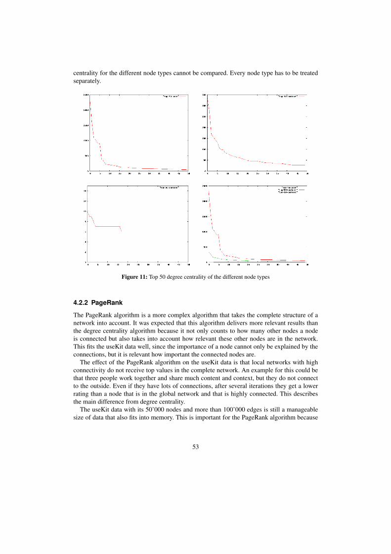
centrality for the different node types cannot be compared. Every node type has to be treatedseparately.

Figure 11: Top 50 degree centrality of the different node types

4.2.2 PageRank

The PageRank algorithm is a more complex algorithm that takes the complete structure of anetwork into account. It was expected that this algorithm delivers more relevant results thanthe degree centrality algorithm because it not only counts to how many other nodes a nodeis connected but also takes into account how relevant these other nodes are in the network.This fits the useKit data well, since the importance of a node cannot only be explained by theconnections, but it is relevant how important the connected nodes are.

The effect of the PageRank algorithm on the useKit data is that local networks with highconnectivity do not receive top values in the complete network. An example for this could bethat three people work together and share much content and context, but they do not connectto the outside. Even if they have lots of connections, after several iterations they get a lowerrating than a node that is in the global network and that is highly connected. This describesthe main difference from degree centrality.

The useKit data with its 50’000 nodes and more than 100’000 edges is still a manageablesize of data that also fits into memory. This is important for the PageRank algorithm because

53

all intermediate results have to be stored. PageRank is an iterative method and already afterfour to five iterations most top ten nodes were under the top ten. The more iterations weredone, the more accurate the results.

To calculate PageRank, the undirected useKit graph was converted to a bidirectional graphwhere every single edge is replaced by two directed edges. The discovery was made that thePageRank results are similar to the degree centrality results, but not equal. This similarity canpartially be explained by the simplified version of the PageRank that was used. Hotho et al.already discovered that the PageRank does not fit undirected graphs that well and proposed animproved algorithm based on the PageRank for undirected graphs, especially for folksonomynetworks, the so-called FolkRank [97] algorithm. The useKit data graph with its context nodeswhich are partially similar to tags is similar to a folksonomy graph. To improve the results, theFolkRank algorithm could be applied to the given data. This was not done anymore becauseof time restrictions.

Also with the PageRank algorithm, content objects do not appear in the top 100 rankings.With the PageRank algorithm this could be the case if a content object has connections toimportant users and context objects. Still it is not likely that a content object appears in thetop rankings because of its few connections, compared to users and contexts. In order to findrelevant or central content objects it could be necessary to only compare the values of the con-tent objects with each other. Having an important or central content would mean this contentis relevant for different contexts / subjects and is important for lots of users (owned by theusers).

A personalized PageRank on the useKit data could be interesting for delivering relevantsearch results to the user. Every user receives the results that are more relevant for him, whichmeans in this case data that is close to the user. A personalized PageRank can also be used forrecommendations. There can be contexts that have a high PageRank seen from this specificuser. If this user did not subscribe yet to the context, this context could be recommended tothe users because he is probably interested in this context. But for recommendations, there aremore relevant factors, such as closeness or access rights. In an implementation of a person-alized PageRank it would be important to only analyze edges to objects where the user hasaccess to. In the current implementations, all edges are analyzed independently of whether thenodes are globally accessible or not.

4.3 Storage systemsEight different storage systems were analyzed for the storage, querying and processing of so-cial data, specifically the useKit data set. The analyzed systems differ in the structure that datais stored, in the query languages and in how data can be processed. There is no clear resultwhich system is the best; it depends on the use case. For the need of processing whole data sets,storage systems which directly implement processing based on MapReduce or other process-ing languages have a clear advantage. Systems with different indices have a clear advantageif querying for single nodes with specific attributes is necessary. The results for every storagesystem for data model, social data, queries and data processing, degree centrality, PageRankalgorithm and scalability are described below.

54

4.3.1 Data model

The data that had to be stored was the same for all storage systems. It was given by the useKitnodes and their relations. The data was modeled differently for every system, as shown insection 3.3.

MySQL with its normalized data model, which is typical for RDBMS, allows to store datain a compact way. Every data entry is only stored once, whereas in other systems e.g. edgesare stored twice or more. MySQL offers good capabilities for querying a specific node in onetable. The structure had to be predefined with tables and columns. Changing the structure inbig data sets can take a long time, which makes the systems inflexible.

As an enhanced key-value store which supports lists, sets and range queries, Redis requiresto model the data differently from MySQL. Modeling data for Redis or key-value stores ingeneral often means creating keys that describe the value stored by concatenating strings. It isimportant that these keys can be recreated for data retrieval. Often, it is necessary to store a listof all ids in advance under one specific id to retrieve all ids later. For this, Redis also offers thekeys command, which makes it possible to retrieve all keys with a specific prefix. The samedata often has to be stored under several keys because no join queries or queries in general areavailable. This can lead to the problem that if data entries are updated, they have to be updatedin different locations. In the useKit data this is the case for the relationships that are storedwith every node. This means that every relationship is stored twice. Updating all data entrieshas to be implemented by the developer and is not supported by the storage system.

Riak, which is also a key-value store, does not support lists or sets but has a native supportfor JSON documents. This makes it possible to use Riak similarly to a document store. Also,the used data model is the same as for document stores. Less complex key constructs have tobe used for Riak than Redis because lists and additional informations can directly be storedinside the value of every node. This allows a flexible data model because no indices have tobe changed or recreated when the data model changes. Riak supports links between the keys.However, this was not used because of limitations that exist with links like the maximumnumber of links that can be sent in the request header.

The two document stores MongoDB and CouchDB use the exact same data model. For bothsystems, the data can be modeled in JSON/BSON, which is also used in Riak. This makes itpossible to model semi-structured data and every node with all its information. Furthermore,edge information is stored in one single document. Connections between two nodes are storedin both nodes and therefore in two documents. If an edge is removed, two documents have tobe updated. Once again, this has to be done by the developer on the client side.

HBase and Cassandra as column stores allow to model the data in a semi-structured waysimilarly to the document stores and Riak. Every node was stored as one row and all additionalinformation was stored in column families and columns including all edges of a node. Incontrast to document stores, column families for both systems had to be predefined, whichmakes these systems less flexible for data modeling compared to document stores. One columnfamily in every row was used to store all adjacency information, which made it possible toupdate and retrieve these values without affecting other values. Cassandra with its support forsuper columns allows to store data in an even more structured way and offers more specificqueries then HBase. During modeling data for column stores it is important to know in advance

55

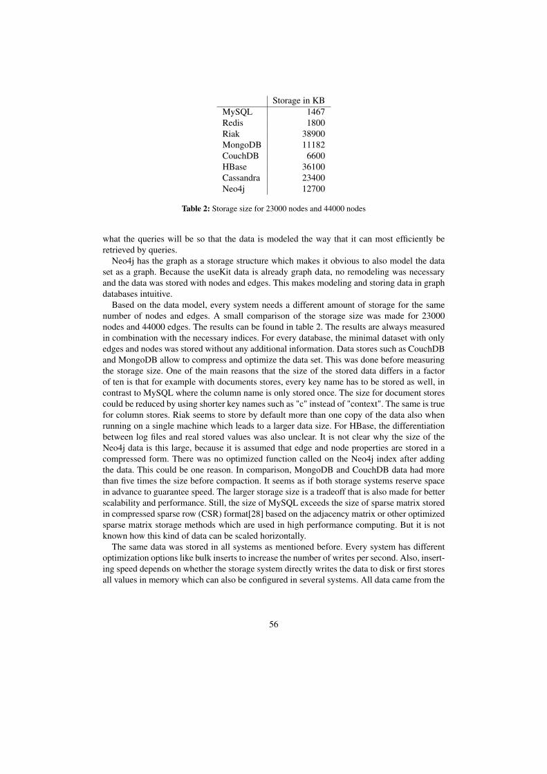
Storage in KBMySQL 1467Redis 1800Riak 38900MongoDB 11182CouchDB 6600HBase 36100Cassandra 23400Neo4j 12700

Table 2: Storage size for 23000 nodes and 44000 nodes

what the queries will be so that the data is modeled the way that it can most efficiently beretrieved by queries.

Neo4j has the graph as a storage structure which makes it obvious to also model the dataset as a graph. Because the useKit data is already graph data, no remodeling was necessaryand the data was stored with nodes and edges. This makes modeling and storing data in graphdatabases intuitive.

Based on the data model, every system needs a different amount of storage for the samenumber of nodes and edges. A small comparison of the storage size was made for 23000nodes and 44000 edges. The results can be found in table 2. The results are always measuredin combination with the necessary indices. For every database, the minimal dataset with onlyedges and nodes was stored without any additional information. Data stores such as CouchDBand MongoDB allow to compress and optimize the data set. This was done before measuringthe storage size. One of the main reasons that the size of the stored data differs in a factorof ten is that for example with documents stores, every key name has to be stored as well, incontrast to MySQL where the column name is only stored once. The size for document storescould be reduced by using shorter key names such as "c" instead of "context". The same is truefor column stores. Riak seems to store by default more than one copy of the data also whenrunning on a single machine which leads to a larger data size. For HBase, the differentiationbetween log files and real stored values was also unclear. It is not clear why the size of theNeo4j data is this large, because it is assumed that edge and node properties are stored in acompressed form. There was no optimized function called on the Neo4j index after addingthe data. This could be one reason. In comparison, MongoDB and CouchDB data had morethan five times the size before compaction. It seems as if both storage systems reserve spacein advance to guarantee speed. The larger storage size is a tradeoff that is also made for betterscalability and performance. Still, the size of MySQL exceeds the size of sparse matrix storedin compressed sparse row (CSR) format[28] based on the adjacency matrix or other optimizedsparse matrix storage methods which are used in high performance computing. But it is notknown how this kind of data can be scaled horizontally.

The same data was stored in all systems as mentioned before. Every system has differentoptimization options like bulk inserts to increase the number of writes per second. Also, insert-ing speed depends on whether the storage system directly writes the data to disk or first storesall values in memory which can also be configured in several systems. All data came from the

56

MySQL database, which limits the insert rate of all other systems by its reading speed. Thus,the performance of writing the data set to the different storage systems was not measured.The results would not be meaningful without making detailed investigation into optimizingevery single system for the use case. To compare the performance in detail, the Yahoo! CloudServing Benchmark (YCSB)57 can be used. This is based on the YCSB paper from Cooper etal.[66].

4.3.2 Social Data

For social data, storage systems with semi-structured data models have a clear advantage be-cause of their possibility to scale and also because social data is often only semi-structured.Column stores are a good fit for lots of social data because column stores are in this thesis con-sidered to be a combination of key-value stores and document stores with tradeoffs. Columnstores are almost as scalable as simple key-value stores but are able to store semi-structureddata with simple indices which allows to do simple queries like range queries. Also the supportfor processing the data with MapReduce is important. This does not mean that column storesare the solution for social data. Every implementation is different and has different goals. Ithas therefore to be evaluated in detail what is needed and where some tradeoffs have to bemade. It is important to know in advance what the requirements will be and what kind ofqueries have to be used in order to choose the right system. As shown in this thesis, every datacan be modeled for every system but it behaves differently for processing, high read or writeloads or for simple queries.

Storing social data in MySQL is not a concern because in general, it is always possible tonormalize data. Typical n to n relations can be represented with additional tables. The costfor writing data to the storage system stays constant because only a row has to be added andsome indices have to be updated. One main concern for using MySQL with social data canbe that the data set can change often, which means the structure of the database has to bechanged. This can be a major disadvantage on MySQL because changing the structure withmuch data can take up to hours. Another problem of using MySQL for social data are thequeries of n to n relationships. With social data, there are often queries that access severaltables which means doing joins in SQL over several tables with large data sets. Because forsome joins the complete data set has to be scanned, this becomes more and more inefficientwith large data sets. An example for such a query could be "All content that is in context 5 andis owned by user 2". For this, a query on the content with two joins to the content_context andcontent_user table are necessary. These joins get slower with large data sets, especially whenthe intermediate results no longer fit into memory.

Redis is not a typical match for social data because it does not directly allow complex datastructures or support queries. Because it allows to store any type of data that can be convertedto a string as values for a key, it is possible to store JSON strings inside Redis. This makes itpossible to use it similarly to Riak. The main problem is that there are no indices or queriesthat can be used to retrieve the data or even to process the data.

Riak fits social data well, especially because it is easy to scale to a large number of nodes. Itis therefore possible to store large data sets and MapReduce queries are supported. The support57Yahoo! Cloud Serving Benchmark project code: https://github.com/brianfrankcooper/YCSB/

wiki/

57

for native JSON documents in every value makes it possible to use it partially like a documentstore and semi-structured data can be stored. In addition, links between keys are possible,which allows link walking which can be typical for some types of data queries in social data.One disadvantage of Riak for social data is that all queries are based on MapReduce, whichmeans that queries are delayed and data cannot be retrieved based on indices or range queries.This will probably change in the future with Riak 0.13 and its Lucene implementation.

With the open data model of MongoDB and CouchDB, almost every type of social datafits the systems. MongoDB with its support for SQL-like queries based on predefined indicesand additional MapReduce queries is an interesting match for social data. The same is true forCouchDB where queries are based on MapReduce but are updated in real time, which makesit possible to retrieve data without additional processing. Both systems have to make tradeoffsfor scalability because scaling in both systems is based on replication and sharding. However,sharding is often a complex task for social data because of its distributed nature.

Column stores fit social data well because of its semi-structure data model and its abilityto scale. Both HBase and Cassandra are a good match for social data because they allowbasic range queries based on (super) column families and also processing of data based onMapReduce with Hadoop is already supported by the system. Both systems can scale to largedata sets.

Concerning the data model, Neo4j fits social data perfectly. One of the main reasons whygraph databases are not largely adopted in social networks is because of its scalability issuesand because most queries are not graph traversal queries. Most queries in social networksare single node queries or range queries. Neo4j does not offer special indices for this kind ofqueries which are not graph traversal queries for which Neo4j is optimized. The graph storagestructure also makes scaling a difficult task. This makes Neo4j a good solution to store socialdata, but not to retrieve social data in a typical way.

4.3.3 Queries & Data Processing

In the implementation, there were no typical social data queries such as the content log on theuseKit start page. The query to get this content log described in words is as following: Getall data that is in all contexts the user has and order it by date. For such queries once again adifferent evaluation of the systems would be necessary. These queries affect only a part of thedata set an can be positioned between the simple degree query and the PageRank processingwhich affects the complete data set. One of the most often used systems for data processing isprobably Hadoop, which directly supports MapReduce. But also additional languages such asPig58 or Hive59 exist. More and more storage systems offer a plugin or adapters for Hadoopthat allow to send the stored data to Hadoop for efficient processing, which is already done inCassandra.

The evaluated systems supported four different types of queries, as can be seen in table3: key requests, SQL queries, range queries and MapReduce queries. MapReduce queriesare already data processing and would also allow to model range queries. Key requests aresupported by all systems, whereas for Neo4j an additional Lucene index is necessary.

58Pig project: http://pig.apache.org/59Hive project: http://wiki.apache.org/hadoop/Hive

58

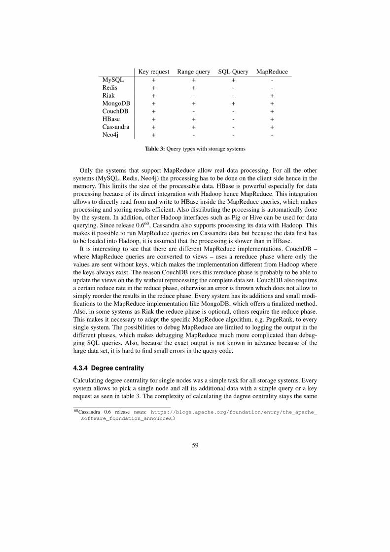
Key request Range query SQL Query MapReduceMySQL + + + -Redis + + - -Riak + - - +MongoDB + + + +CouchDB + - - +HBase + + - +Cassandra + + - +Neo4j + - - -

Table 3: Query types with storage systems

Only the systems that support MapReduce allow real data processing. For all the othersystems (MySQL, Redis, Neo4j) the processing has to be done on the client side hence in thememory. This limits the size of the processable data. HBase is powerful especially for dataprocessing because of its direct integration with Hadoop hence MapReduce. This integrationallows to directly read from and write to HBase inside the MapReduce queries, which makesprocessing and storing results efficient. Also distributing the processing is automatically doneby the system. In addition, other Hadoop interfaces such as Pig or Hive can be used for dataquerying. Since release 0.660, Cassandra also supports processing its data with Hadoop. Thismakes it possible to run MapReduce queries on Cassandra data but because the data first hasto be loaded into Hadoop, it is assumed that the processing is slower than in HBase.

It is interesting to see that there are different MapReduce implementations. CouchDB –where MapReduce queries are converted to views – uses a rereduce phase where only thevalues are sent without keys, which makes the implementation different from Hadoop wherethe keys always exist. The reason CouchDB uses this rereduce phase is probably to be able toupdate the views on the fly without reprocessing the complete data set. CouchDB also requiresa certain reduce rate in the reduce phase, otherwise an error is thrown which does not allow tosimply reorder the results in the reduce phase. Every system has its additions and small modi-fications to the MapReduce implementation like MongoDB, which offers a finalized method.Also, in some systems as Riak the reduce phase is optional, others require the reduce phase.This makes it necessary to adapt the specific MapReduce algorithm, e.g. PageRank, to everysingle system. The possibilities to debug MapReduce are limited to logging the output in thedifferent phases, which makes debugging MapReduce much more complicated than debug-ging SQL queries. Also, because the exact output is not known in advance because of thelarge data set, it is hard to find small errors in the query code.

4.3.4 Degree centrality

Calculating degree centrality for single nodes was a simple task for all storage systems. Everysystem allows to pick a single node and all its additional data with a simple query or a keyrequest as seen in table 3. The complexity of calculating the degree centrality stays the same

60Cassandra 0.6 release notes: https://blogs.apache.org/foundation/entry/the_apache_software_foundation_announces3

59

for all systems and also for growing data sets. To compare and order all the results, the storagesystems which support processing the data with MapReduce had a clear advantage because onthe other systems the processing had to be made on the client side.

MySQL performed well for calculating degree centrality, especially if the degree centralitywas requested for only one node. To return degree centrality, only two indices have to beaccessed and two counts have to be made. The response time and the complexity stay constantfor such queries even if the data set grows. This is different for querying the top ten degreenodes. MySQL therefore first has to execute the two queries mentioned before for every singlenode, store the results in memory and then order the results. This has to be done every time arequest is sent to the server, because intermediate results are not stored. The amount of workthat has to be done grows linear with the amount of data. The time needed for processing alsogrows in a linear way as long as all intermediate results can be kept in memory. As soon as itis necessary to write intermediate results to disk, it gets slower by a large factor. It was triedto create a view based on the presented queries. However, in MySQL these views were evenmore inefficient than doing the queries directly because it seemed like MySQL does not useall indices correctly to calculate the results. As read this could be different with other SQLsolutions like PostgreSQL or Oracle. MySQL does some internal query caching, but this wasignored in these experiments.

In Redis, degree centrality can be calculated quite simply because all links from one nodeto other nodes are stored in two lists. To calculate degree centrality for a node, only two countrequests have to be made. Getting the degree centrality for all nodes is more processing andquery intense because it has to be done for every single node and ordering would have to bedone on the client side. If the top ten degree nodes would be needed it could be implementedthe way that a sorted set is created with every node inside and the degree as the score. Everytime a node is updated, the list has to be updated with the new values. Once again this wouldhave to be implemented by the coder on the client side.

In Riak, MongoDB, CouchDB, HBase and Cassandra, degree centrality is easy to calculatefor a single node because all data needed for calculating degree centrality is stored in a singlevalue, document or row. With one request, the data can be retrieved and in the Java code thelength of the adjacency array can be retrieved. For processing and comparing degree centralityof all nodes in all systems, the same MapReduce queries shown in section 3.2.1 are used. Inthese systems only the results have to be retrieved by the client and no processing is neededon the client side in contrast to MySQL, Redis and Neo4j.

Degree centrality calculation on Neo4j for one node is simple because every node knowsall its adjacencies. Calculating degree for all nodes and comparing it cannot be done in thestorage system and has to be done on the client side as with MySQL and Redis.

4.3.5 PageRank

For the PageRank processing, once again the systems which support MapReduce queries havea clear advantage because on the other systems, the calculations have to be done on the clientside which leads to much communication between the storage system and the client becausethe client has to retrieve the complete data set. In addition, the client has to be capable ofkeeping all data in memory to process it, which is not possible for large data sets.

60

On MySQL, the PageRank algorithm was partially implemented for testing on the clientside. All data was queried from the storage system and then processed by the serial PageRankalgorithm. The implementation was made in Java. There are two options for the algorithm.One is to make the calculations for every separated node and write the intermediate results toa special storage place which also means that information for a single node has to be queriedseveral times and at the end of every calculation, the intermediate results have to be writtenback to the storage. The second option is to load all data in memory and directly make allcalculations based on the memory data. This is much more efficient but requires that all datacan be loaded into memory which limits the size of the data. In general this does not scaleto large data sets. The client side calculations based on these two ideas were only made forproof of concept but are not a solution for large data sets. It would be possible to implementthe PageRank algorithm as a stored procedure in MySQL. But then it would still be neces-sary to call the stored procedure on every single row and it would be necessary to store theintermediate results somewhere. This was not done in the experiments.

On Riak, MongoDB, CouchDB, HBase and Cassandra, the PageRank implementation wasdone based on MapReduce. The basic MapReduce code is the same in all systems as pre-sented in listing 4 but the parameters and capabilities of every system differ in the details asdescribed before. The most powerful, simplest and most efficient solution is the implementa-tion based on HBase in combination with Hadoop. Data can be read and written to the storagesystem directly in the MapReduce code and it is possible to add multiple reduce steps or to runmultiple iterations with a single call to the system. Because the MapReduce queries are imple-mented in Java, the complete capabilities of the Java language can be used. Riak, MongoDBand CouchDB in contrast implement the queries in JavaScript which also allows almost allpossibilities Hadoop offers but it would not be possible to access external data in some specialcases as it is possible with Hadoop. This was used to create the output for the plots. Therewas no implementation for Cassandra, but the processing would be done in the same way aswith HBase and Hadoop. Even though there were not made any performance comparisons, theperformance of the PageRank processing was the fastest on Hadoop and was much slower onthe other systems. All processing was done on a single machine which makes it impossible tojudge how the different systems would behave and perform on multiple machines. One maindisadvantage that was found in Riak is that there was no way to directly write back the data tostorage from the reduce phase instead of sending it to the client first, which heavily degradesthe performance.

4.3.6 Scalability

All installations and tests were made on only one or two machines. Because of this, no clearrecommendation can be made which systems scales best in which cases, but assumptions aremade based on the knowledge about the storage systems. Here, scaling means scaling to alarge amount of data which is stored on several machines. It is important not to confuse it withperformance. All systems are able to scale reads by replication. The less structured the data,the simpler scaling is where key-value stores are at the one end and RDBMS on the other end,as can be seen in figure 12.

As can be seen in table 4 the different systems support different methods to scale to largedata sets. Replication is supported by all systems by which reads can be scaled and the data is

61

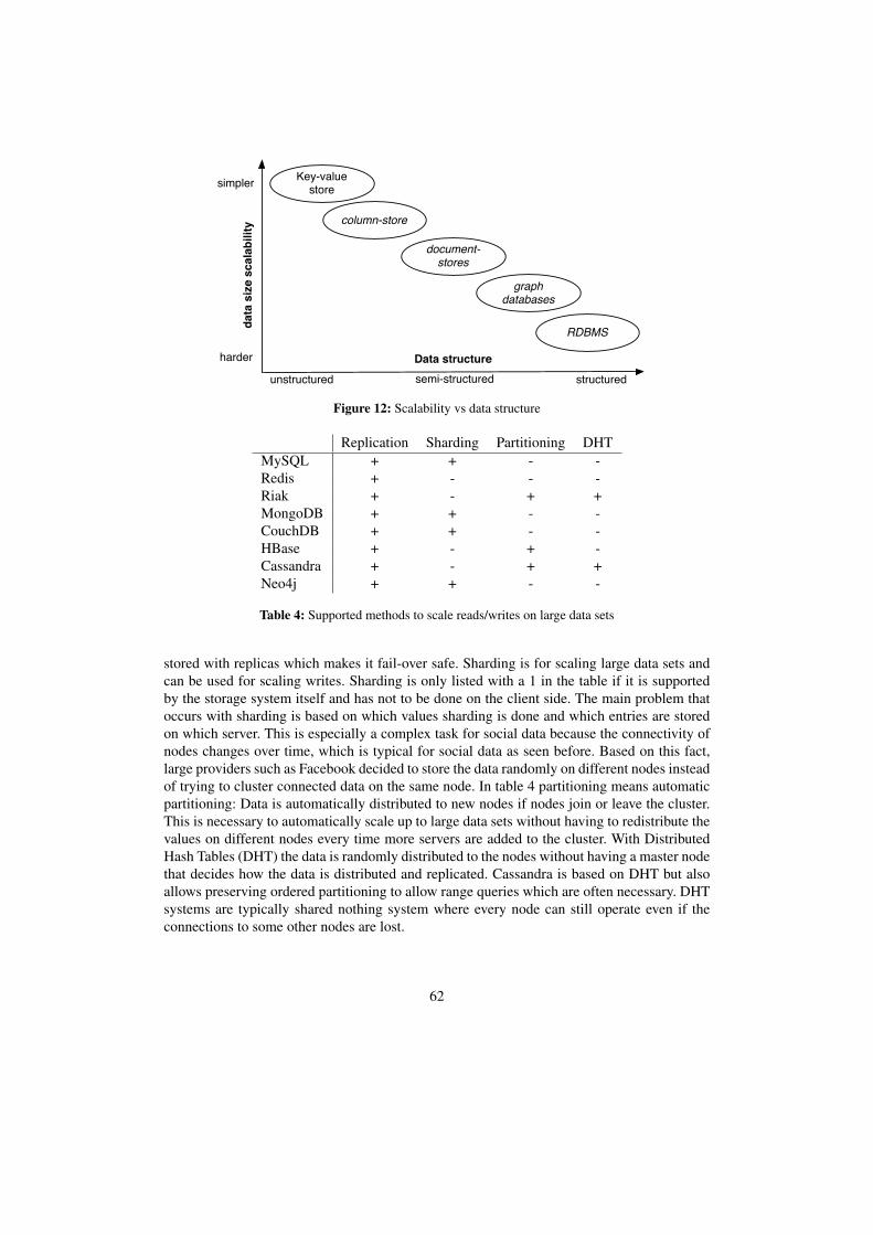
Data structureunstructured structuredsemi-structured

simpler

data

siz

e sc

alab

ility

harder

Key-value store

column-store

document-stores

graph databases

RDBMS

Figure 12: Scalability vs data structure

Replication Sharding Partitioning DHTMySQL + + - -Redis + - - -Riak + - + +MongoDB + + - -CouchDB + + - -HBase + - + -Cassandra + - + +Neo4j + + - -

Table 4: Supported methods to scale reads/writes on large data sets

stored with replicas which makes it fail-over safe. Sharding is for scaling large data sets andcan be used for scaling writes. Sharding is only listed with a 1 in the table if it is supportedby the storage system itself and has not to be done on the client side. The main problem thatoccurs with sharding is based on which values sharding is done and which entries are storedon which server. This is especially a complex task for social data because the connectivity ofnodes changes over time, which is typical for social data as seen before. Based on this fact,large providers such as Facebook decided to store the data randomly on different nodes insteadof trying to cluster connected data on the same node. In table 4 partitioning means automaticpartitioning: Data is automatically distributed to new nodes if nodes join or leave the cluster.This is necessary to automatically scale up to large data sets without having to redistribute thevalues on different nodes every time more servers are added to the cluster. With DistributedHash Tables (DHT) the data is randomly distributed to the nodes without having a master nodethat decides how the data is distributed and replicated. Cassandra is based on DHT but alsoallows preserving ordered partitioning to allow range queries which are often necessary. DHTsystems are typically shared nothing system where every node can still operate even if theconnections to some other nodes are lost.

62

Every system has its advantages and disadvantages in scaling. It is important to know if onlyreads or also writes have to be scaled. Redis is limited in scaling to large data sets because theperformance of Redis is based on the assumption that all data can be kept in memory. Shardingto different nodes is not supported yet, but should be added in one of the next releases. HBaseuses a single master name node to manage the different nodes which adds on single point offailure, but HBase allows to have multiple master nodes which means replicas of the namenode exist and an automatic fail-over can happen if the master fails. Cassandra on the otherside does not need a master node because all nodes are equal and new nodes are discoveredautomatically. There is no single point of failure. Cassandra scales better for writes than HBasebecause of its eventual consistency. This makes it possible to still write to the system also ifsome nodes are not available but can lead to inconsistent data that has to be merged. One maindisadvantage of Cassandra is that when the data structure of (super) column families changes,the cluster has to be restarted to support the new data structure. There were not made anydetailed performance measurements but all systems could be improved in speed by improvingand adapting the configuration to the specific use case.

4.3.7 General survey

MySQL has proven to be stable and reliable which makes it a good fit for all relational datawhere transactions or other RDBMS features are needed. Setting up MySQL is simple andrelational databases are still best known by most developers, which makes them a first pickcandidate for most projects.

Redis is a great addition to other storage systems or as a caching solution. It stores simplekey-value data and lists data efficiently and fast. The list feature also allows range queries andatomic operations. The scalability is limited because for good performance the whole data setshould fit into memory. Also automatic sharding is not supported yet.

As a key-value store dynamo implementation, Riak makes it possible to scale up to largedata sets with no single point of failure and automatically scales by just adding nodes. Thenumber of nodes used for a read or write can be chosen separately for every request. Its im-plemented support of MapReduce is a necessary addition to process and query data. To storedata redundantly in Riak it is necessary to run Riak on more than one node as all similar dis-tributed systems. The support for JSON documents and links which allows link walking isa great addition for social data. The main disadvantage of Riak is that no range queries arepossible because the data is distributed based on DHT. In the most recent version (0.13) ofRiak Lucene is directly integrated into Riak and supports indices and search queries.

MongoDB and CouchDB are two similar document stores. The data model allows to throwalmost any kind of data into the storage. MongoDB offers a query language similar to SQL(only on not sharded systems) and offers indices that can be set on specific keys. This allows asimple entry point for users that are new to NoSQL solutions. Both systems offer MapReducequeries. CouchDB offers more enhance MapReduce queries because all queries are basedon MapReduce and the system automatically creates indices based on these so-called views.CouchDB is based on the eventual consistency model and MVCC, whereas MongoDB usesstrong consistency. Both systems lack the possibility to automatically horizontally scale writes.

HBase and Cassandra with the column model as storage structure offer a combination ofkey-value store and document store. It allows to store semi-structured data but still allows

63

range and filter queries. The data is distributed based on partitioning or DHT. Because of itsconsistency, HBase is better in high read rates and Cassandra in high writes rates because ofits eventual consistency model. More and more companies pick HBase as part of their storagesolution. This can be for pure processing in combination with Hadoop or – in the case ofFacebook Mail – as storage system. The community around HBase is growing and has somelarge committers such as Yahoo or Facebook. When Cassandra was published by Facebook,it was one of the first scalable NoSQL data stores that were open source. Because of this astrong company grew around Cassandra and there was a lot of buzz around this project. Stillit is under heavy development. But in the meantime other interesting projects were published.It is difficult to predict in which direction the development of Cassandra goes in the future butprobably it is going to stay one of the key players in the NoSQL market.

Neo4j is under heavy development and one of the next large community goals is to makeit more scalable. Neo4j allows to represent network data 1 to 1 in the storage structure whichmakes it intuitive to work with graph data. The various components and extensions makeNeo4j a powerful solution for all graph data where graph traversal is a key issue. Because ofits scalability issues and lack of range queries there is no large adoption of graph databases forlarge data sets yet. Indices and search queries based on node values can be provided by addingLucene indices.

4.4 VisualizationCreating valid dots files was done through Java code directly from the MySQL database.Updating the data if a node or edge changes cannot be done without querying the completefile. Because of this every time the graph changes the DOT file has to be recreated. Processingthe created DOT file was done with the code seen in listing 23 which writes the graph into thefile in the SVG format.

d o t −Tsvg graph . d o t −K n e a t o −o graph−n e a t o . svgd o t −Tsvg graph . d o t −K s f d p −o graph−s f d p . svg

Listing 23: Graph creation command with neato/sfdp

The neato and the sfdp algorithm offered the best visual results for the useKit data. Thespring and the force model approach seem to offer the best results for this kind of social data.Different parameters were tried to optimize the visual output. The parameters which can befound in listing 24 returned the best results. The parameter model=subset is an optimizationfor large graphs developed by Gansner et al [98] based on stress majorization. The parameterpackMode=clust tries to cluster subcommunities, outputMode=edgefirst draws the edges firstand then draws the nodes. Otherwise many nodes could not be seen because an edge is on top.

graph G {model= s u b s e toutputMode= e d g e s f i r s tpackMode= c l u s t

Listing 24: Graphviz params for neato and sfdp

Other parameters such as overlap = false were tried out but this leaded to memory over-flow errors. It is also possible to choose different start nodes but with the size of the graph data

64

no real differences were discovered. It was also tried to show some special nodes like the userNicolas Ruflin or the context Master Thesis. Even though a special form was added to theseedges, they cannot be discovered in the visual output. Another problem occurred when tryingto convert svg files to png. With some large svg result sets this also leaded to out of memoryerrors.

The output of this processing can be seen in figure 13. This output shows the completecommunity structure of useKit. There are some large and heavily connected networks in thecenter. Between these nodes, there are smaller clusters with several users that share contextsand content items. This structure is typical for useKit and represents how useKit is used. Smallgroups work together on a project, produce lots of content and share it over contexts. Ofteninside companies several such groups exist with overlapping users and contexts. Together,these groups form the clusters that can be seen in the figure. On the outside are singular usersthat probably signed up and do not use the useKit platform anymore.

The time needed for creating one visual representation as SVG file was not relevant for thisthesis. The visualization was made of one snapshot of the data set. Most of the processingalgorithms for Graphviz except sfpd support only one processor, which makes scaling theprocessing to large graphs difficult. Throwing lots of memory at the visualization task helpsbecause visualization is much faster as long as all data and intermediate results fit into memory.

One of the main restraints during processing of large graphs was the available memory. Forefficient processing, the whole graph has to be in memory for fast access from the processor.The test environments with 2 and 4 GB of RAM were not sufficient for many algorithms andsome specific parameters. As soon as the data has to be stored to disk, processing gets muchslower. With the growth of fast SSD and growing space of fast memory this will be less of aproblem in the next years. One solution that was used to solve this problem was renting extralarge EC2 instances for a short time period which offers 15GB of RAM and 8 EC2 computeunits. Even larger instances with up to 68.4GB of memory exist. The access to the machine atthe math institute with 48GB of RAM first made it possible to also process and visualize themost recent data with more than 100’000 nodes. Even though most processing was done on asingle processor, the processing time was reduced from more than one hour to several minutes,which showed how important the amount of RAM is for efficient graph visualization.

A possibility to get better visualization results is to shrink the data to only one cluster andthen create the DOT language file based on this data to visualize only one cluster in orderto get a more specific view of the data. If all data is connected without separated subgraphs,algorithms for detecting community structures are needed. This can be an expensive task.

The data was processed without time constraints. This means it was ignored when a specificconnection between two nodes was created. If a user created lots of content and contexts abouta year ago and is now not active anymore, he can still appear on top of all users even if he isno longer active in the system. For better results a time factor should be used that only showsactive data or data that was changed or created recently.

Visualizing data well is a time-consuming task. Tools like Graphviz are helpful to visualizelarge graph sets and also to deliver good basic results. To improve the outputs, lots of parame-ters can be set. The output after processing cannot be predicated completely for large graphs,which often makes it a trial and error approach. Improving automation of graph visualiza-tion would lower the entrance hurdle for lots of other research areas to visualize and betterunderstand their data sets.

65

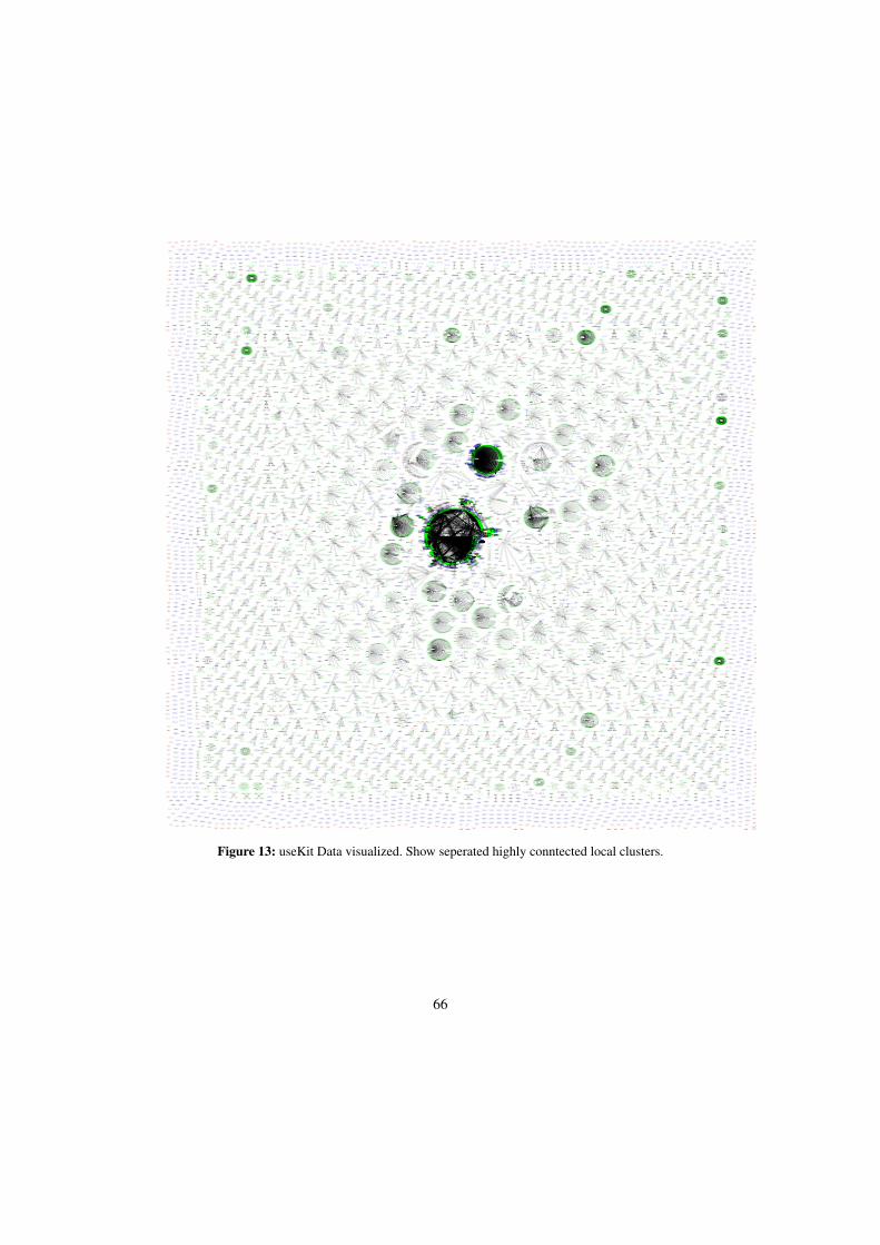
Figure 13: useKit Data visualized. Show seperated highly conntected local clusters.

66

5 Discussion & Future WorkThis section will be concerned with the specific results from the analysis and results part. Inaddition, some ideas for future work will be discussed for every research area.

5.1 DataThe main challenge with social data is its structure and its size. The structure of single nodesvaries from use case to use case, but also the global structure of every network is different. Ev-ery social network is unique and to analyze a network, first the structure has to be understood.There are approaches to standardize some representations such as friendships with FOAF. Thisshould also help to make data portable from one platform to another. Much more important toexchange data are the APIs that are offered by most platforms which are not standardized butallow to access the data from a social network in a simple way.

Even if the structure of social data changes and exists in various forms, the basics stay thesame: Nodes are connected through edges. New types of social data such as location data frommobile devices but also sensor data, which will also be part of the social data stream, growfast [58]. The amount of data that is produced daily already exceeds the amount of data thatcan be stored, and the gap between created data and storage capacity will grow larger over thenext few years. Processing the data efficiently and only storing the relevant parts will get moreand more important and in general the importance of graphs will rise.

Because there will not be any predefined structure of social data and the amount of datawill grow, this poses special requirements on the storage systems. There will be specific andoptimized solutions for every social network and probably less standardization because per-formance is more important and standardization always means making some tradeoffs.

The analyzed useKit data set is only a specific case. As it was already discovered with theuseKit data set, the structure changes over time and new types of edges and nodes are added tothe data set. This often happens when new features are added to a social platform. More socialnetworks should be analyzed based on the node and overall structure and some classificationschemes should be developed to classify the social networks into different groups to find outif some general structures exist.

One main challenge with social data is the querying of social data. This is connected to thestructure of social data, but was not discussed in detail in this thesis. Typical news feed streamsas can be found on the Twitter or Facebook start page were not discussed in this thesis. Thesestreams consist of data from connected nodes and poses a real challenge to storage systems inorder to retrieve this data. It would be interesting to do more research in this area to find outhow these feeds can be created in an efficient way.

5.2 Storage systemsPlatforms such as Facebook or Google are already capable of storing and processing an im-pressive amount of data. Facebook has more than 500 million users, only a fraction of theusers is online at the same time. There are no web applications yet that allow a large amountof the world population to interact at the same time. This world scalability will become more

67

and more important as more and more users are online at the same time all around the worldwith their mobile devices.

Five different types of storage systems were evaluated. There is no single system that isbest in all parts, since every system has its advantages and disadvantages. This is typical forso-called NoSQL solutions because most systems were developed with a specific use casein mind. A question that is raised frequently concerns standards for NoSQL solutions, forexample for a query language similar to SQL. It is assumed that there will not be any querystandards that can or will be adopted by most of the systems. One reason is that most ofthese systems were built because other systems were not good enough in a specific task, sothese systems were built to solve these tasks best. Standardization often has the drawback ofloosing some performance, which is the opposite of what these systems were built for. Onestandardization that is already part of most systems is the access interface. REST is chosen inmost systems as one of the access methods. This makes it possible to use the systems fromall kind of client languages and to use all these systems in service-oriented architectures andover network connections. NoSQL solutions do not directly compete with traditional SQLsolutions. The discussion if NoSQL replaces SQL is needless. There are needs for both kindsof systems. The goal is to pick the best system for every task. This can also mean that oneplatform uses different systems for different data sets. NoSQL solutions are not yet as stableas SQL solutions. The reason for this is that most systems are still in early development andare in alpha or beta stage. It will take some more time to mature these systems. At the moment,a new system appears almost every week in the community. In the long run probably only thebest and most stable system will survive.

One main concern with most NoSQL solutions is that there is no or only limited accessmanagement. This can be a security issue. However, most systems started to implement rudi-mentary access management; HBase can be taken as an example. But there won’t be the samefine-grained access management like in most SQL solutions based on tables or even rowsbecause checking access rights for every read and write can be a scalability issue in largesystems.

An interesting new movement can be seen in CouchDB. CouchDB can be used on mobiledevices and can distribute data over several mobile devices or sync the database betweendifferent systems. This indicates that in the future, mobile devices will probably also be partof the global storage cloud. This poses new problems such as high latency or disconnectivityto storage systems. This approach is sometimes also mentioned as the ambient cloud [99].Already now, most scalable implementations of data storage and data processing are basedon commodity hardware that is scaled up to thousands of nodes across different data centersinstead of using super computers. This approach will even be extended by the ambient cloudwhere resources could be used and shared across the globe, including mobile devices.

Social data has a diverse structure and the actual need differs heavily from use case touse case. The selection of the storage system depends heavily on the actual problem. Therequirements such as data size, consistency, availability or how the data has to be queried,processed or searched have to be known in advance to make a decision for the right system.

Every system had its specific advantages and disadvantages in storing the data as was seenin the results and analysis section. Column stores seem to be one of the systems that fit bigdata or social data best. Column stores are a combination of document stores and key-valuestores. The data structure has to be only partially predefined and data is accessed directly

68

through keys or range queries. No complex query systems exist. Column stores are built tobe scalable. HBase with the HDFS file systems as backend, Hadoop for data processing andseveral extensions such as Hive and Pig to query the data, this seems to be one of the mostpowerful systems to scale and process big data at the moment.

The main concern with SQL solutions is that scaling is more difficult and the systems arenot built to process large data sets. As soon as large data sets have to be stored, several serversor complete data centers are involved. This means that nodes will fail on a regular basis andreplication of all data is necessary. Cassandra offers a scaling structure where every node isexactly the same and no central master exists which means no single point of failure. Thismakes adding and administering nodes simple. On the downside, this also means that there isno central point of control.

Having different storage systems for the same data can be a big advantage as was experi-enced during the experiment. To process data, it is nice to have systems such as HBase thatsupport MapReduce queries. Doing graph traversal in such a system would be difficult. Hav-ing the same data also stored in Neo4j makes it simple to write some graph traversal queries.In real implementations it is not applicable to always have all data in different storage systems.But it is worth thinking about having importers for other systems to process and query the datain other systems instead of writing complex systems to process the data as is necessary.

Another interesting aspect would be to compare the performance of the different systems.However, doing good and relevant benchmarks is a difficult task and was – due to lack of time– not part of this thesis. Benchmarks always have to be done with a specific data set and itsrequirements. To choose a system that fits the given data and requirements, deep understandingof the data is necessary and it has to be known how the data will be accessed. Some systemsare better in inserting/writing data, others in reading. Easy insert does not necessarily meaneasy out which is typical for key-value stores where adding data is simple but it has to bethought in advance how to retrieve the data again. Basic questions need to be asked such as: Isit more read or write oriented? Should availability or consistency be chosen? Picking the rightsystems is a long process. There is not one system that fits all needs. Always the system thatfits the problem best should be chosen.

There are strong communities around these new storage solutions that are lead by the highlyskilled developers of the storage systems. This often leads to interesting discussions wherethe systems are compared and where it is seen that similar problems were often solved withdifferent approaches. Because there is also a hype around these systems, a lot of blogging isdone where also false information or outdated information is posted. This sometimes leads toconfusion in the community. Especially subjects such as the basic CAP theorem is a subjectthat is often discussed and a lot is written about.

Having the same data in different storage systems makes it possible to always use the mostefficient system or the simplest one to implement a certain task. Selecting and evaluating singlenodes is simple and efficient in MySQL. This makes debugging and searching single nodessimple. Batch processing with MapReduce is implemented well in HBase/Hadoop which madeit simpler to write this code for HBase first and then adapt it to other systems. There are alwaysdifferent problems that have to be solved for one data set. This can make it reasonable to storethe data in the different storage systems.

Even though there already is a fair amount of storage systems, more research should bedone in this area to create even more scalable systems. Especially the combination of storage

69

systems with processing should be researched in more detail in order to provide more efficientprocessing methods.

5.3 Processing / AnalyzingIn this thesis, the aspect of retrieving items from a database and processing the data afterretrieving was looked at. One important case that was not discussed is searching inside thedata. The de facto standard in this area is Lucene. Searching through data sets once againposes different requirements on the storage systems. Data is analyzed first and then stored ina form that it can be searched easily. Most of the systems mentioned before have plugins orexport scripts to send data directly to Lucene.

Different types of centrality were calculated for the different types of vertices. First, degreecentrality was calculated. For this multidimensional type of data, it was clear that the degreecentrality would only give a basic idea about a vertex. For a user it describes how active thisuser is in creating content and creating / subscribing to contexts. But it does not describe therole or position of the vertex in the overall network. The reason for this is that to evaluate theposition or role of a vertex with the given data, at least the next node is relevant. It is possiblethat a user created 100 content items and 10 contexts without having a connection to any otheruser over a context or a content item because all contexts are set private.

The PageRank algorithm is useful in directed graphs data sets like web links, but has itslimitations for undirected graphs. The results delivered by the simplified PageRank algorithmsare still relevant but could be improved by making modifications on the algorithm in orderto better fit the undirected graph and the useKit data set like the FolkRank [97] approach.Facebook – as one of the largest networks with an undirected graph – has not yet revealed anyalgorithms about the calculation of the centrality of a person in the network, and especially itsfeed creation, which is a combination of different items from connected users. Which exactitems are shown is based on algorithms which Facebook once called EdgeRank61. Still a lot ofresearch is needed in the area of centrality measures and undirected graphs in order to providebetter centrality measure for undirected graphs or even graphs that consist of a combination ofdirected and undirected edges. There do not exist any algorithms similar to PageRank whichdeliver relevant results for graphs that have both types of edges, directed and undirected ones.

The useKit data set was processed for degree centrality and a basic PageRank algorithm.The results of both algorithms were similar and showed the central nodes in the graph foreach type of node. All node types in the useKit graph were treated equally. Even though someexperiments were made in weighting the edges differently between the different edge typesthis was not treated concludingly. More research in this direction should be done to evaluatehow the different node types and edge weights can affect the graph processing.

For all this processing, only the basic information was used. The useKit data would offermore factors based on which a more fine-grained processing would be possible. For contentitems, the number of views and additionally the number of comments could be taken intoaccount. For a context node, the number of views could be added. In the original data set, auser is also directly connected to other users which could be added to the processing info. To

61f8 developer conference video mentioning EdgeRank: http://apps.facebook.com/feightlive/

70

process this information, advanced algorithms would be needed. This would probably delivermore fine-grained results.

The processing of the nodes was made independently of the time in which a node or an edgewas created. In social networks, information often depends on its actuality. So the date of thenodes and the edges should also be a processing factor in future experiments. This additionalinformation would also exist in the original data set. Interesting and more relevant resultscould be retrieved by extending the PageRank algorithm also with date information, whereasolder information would be less relevant.

All the data was processed based on a global view on the graph. By processing local sub-graphs, recommendations could be made to show a user contexts that he could be interestedin. Another possibility is to recommend users with similar interests which are in the samecontext but to which the user does not have a direct connection yet. Identifying similar con-texts could lead to context recommendations for content items. For this, different processingmethods would be needed that were not evaluated in this thesis.

There are different approaches to data processing, such as incremental processing or batchprocessing. Until recently, large data processing was mostly done with the de facto standardMapReduce. After updating parts of the data, it was necessary to reprocess the complete dataset. It was already known that this is not the most efficient way because the same data has tobe reprocessed several times. With the release of Google’s live search and the Pregel paper[12], Google showed that there are already new methods of how large data sets can be updatedin almost real time without having to update the complete data set. Sensor network data willgrow and already more data is produced than can be stored. This makes it necessary to processthe data in real time and only store the relevant parts. Data processing is a subject that isclosely connected with data mining and machine learning which makes it interesting in lotsof other areas. New systems such as S4 from Yahoo62 that is based on streaming data try tolower the entrance barrier to make data processing also available to a broader target group.The same is done with alternative processing languages for Hadoop like Hive that offers moreand SQL style of writing queries, or Pig as an alternative that might also simplify the writingof processing queries.

Scaling the processing of large data sets is not easy. There can be different bottlenecks. Itcan be the storage system, network connections or the processing itself. One general discov-ery is that it is tried to move the calculations closer to the data which is known from storedprocedures in RDBMS. But these calculations are horizontally scalable to not become a newbottleneck. At the moment, the most scalable processing system seems to be Hadoop, whichscales up to thousands of nodes.

One of the next steps in data processing is probably to distribute it even more and to useall kinds of idle devices. Mobile devices such as smart phones or tablets have more and moreprocessing power that could also be used. One of the first approaches that showed how cal-culations can be distributed was Seti@home[100] that used millions of home computers toanalyze data. Wuala63, a swiss start-up that makes it possible to share own disk space to getmore web space, already shows how it can be done for storage space with different kind ofdevices. The same could be done with processing. A user can let his own processing power to

62S4 distributed stream computing platform: http://s4.io/63Secure online storage: http://www.wuala.com/

71

others that need it [101]. This would make large amounts of processing power available thatcould be rented when needed.

A new area of research is graph similarity and graph comparison. Several graph similarityalgorithms are based on PageRank or other centrality measures. One of the goals is to find outwhich communities are similar to others and to describe what that means in detail. There aremany other appliances of graph comparison in biology, medicine, chemistry and other areas.To calculate the results, efficient graph preprocessing is needed based on some algorithms asPageRank shown in this thesis. Once again, for better graph comparison improved centralityalgorithms are need that also deliver relevant result for undirected or mixed graphs and canprocess nodes based on time values or other specific needs.

5.4 Visualization of Graph DataVisualization is a complex subject and research in this area has just started. Creating good out-put images requires a lot of processing power and because it is not only based on algorithmiclogic, user input and tweeking the parameters is needed to get good results that are understoodby people. Visualizing results and data often helps to understand complex results and data sets.

Different approaches were used to visualize the useKit data. The current results is a globalview on all data that differentiates between user, content, context by color. This helped tounderstand the structure of the useKit network. It would be interesting to visualize only sub-graphs or sub communities that are highly connected in order to better understand the localnetwork structure. For this, preprocessing with community detection and subgraph separationwould be necessary. Also interesting would be to show some special nodes in the graph suchas the most popular or relevant users and contexts. This was tried but no helpful output re-sults were produced. Another subject that is popular at the moment because of the 3D cinemawould be to visualize the data in a 3D cube, which makes it possible to fly through the data.Most existing algorithms are optimized to create two-dimensional data. The used formulas ingraph visualization are from physics, for example the electrical spring model or the minimalforce model. The assumption can be made that these models would also work in the three-dimensional space.

All data was visualized independently of time. Thus, a content that was created a year agois shown exactly the same as a content object that was created recently. The assumption can bemade that data which was not updated in a year is probably less relevant than new data. Onepossibility could be to fade out such data points more and more with time or move them in thebackground. Such time-resolved network studies are also called longitudinal studies and areresearched by different research groups at the moment.

The useKit data was visualized at one point in time. It would be interesting to show how thenetwork changes over time. This could be done because a copy of the complete useKit dataset exists from every six hours. However, there are several problems. First, a lot of processingpower is needed to visualize every data set and then to create a movie out of it. A secondproblem could be that the visualizing algorithm decides to visualize the data completely dif-ferently even if only one or two nodes change. For people this would look like a large jumpin the data set. So there should be some constraints that single data points do not move toomuch between every iteration. But to do this, it is necessary to know the previous results andto understand what node was where. A next step would be to visualize the data in real time.

72

The data set is continuously growing, which is why visualizing the data in real time with thecurrent algorithms and processing capabilities is not possible. More research is needed in thearea of live processing data and direct visualization also for large data sets.

Visualizing data is a complex undertaking and a deep understanding of the data is necessarybefore processing and knowledge in the area of visualize algorithm. But visualizing large datasets should be available also to other areas where these requirements are not met. One firststep in this direction is ManyEyes from IBM. This allows people to upload own data sets andvisualize these data sets. Still, a lot of research has to be done so that data sets are automaticallyunderstood by the algorithm in order to set the right algorithms and optimization parameters.This touches also the research area of machine learning because computers have to learn thehuman understanding of a pleasant graph.

73

6 ConclusionThis thesis was concerned with analyzing the structure of social data and discovering whichstorage system fits which type of data best on the basis of concrete implementations. In thecourse of these implementations it was discussed how the data can be processed and analyzedin the respective system. Furthermore, the data set was visualized.

Social data is semi-structured and the structure often changes. Social networks evolve, newfeatures are implemented and new devices such as mobile phones feed data with differentstructure into the social network. This makes it necessary to have adequate storage systemswhich are capable of evolving with the growth and changes of social networks. To betterunderstand the data, centrality measures are necessary in order to identify important nodes inthe network. Through visualization, a complete view on the data set can be produced whichgives interesting insights into the graph structure.

The smallest denominator that is shared by all social networks and social data in general isthe possibility of representing them as a graph. All social data consists of nodes and edges.Depending on the network, the edges are undirected or directed and they can or cannot haveweights. Often, different kinds of nodes with additional properties exist. All these nodes areconnected by edges. Most social data sets are different from web link data sets. Web link datasets are directed graphs and because of their domain structure it is possible to cluster the dataof one domain closely together in the storage system. This is mostly not possible for socialdata because communities that could be similar to domains change and evolve over time. Somecommunities break up and new communities with different connections are built. This makesit almost impossible to store users with similar communities close to each other because theirconnections change over time. Thus, social data poses special requirements to storage systems.

The problem of finding the right storage system for social data has not yet been solved.There is no general solution for social data because, as mentioned before, the structure of ev-ery social data set is different and also the requirements of the different social networks aredifferent. Graph databases such as Neo4j are adequate for storing graphs and for representingsocial data but have constraints in querying and processing social data because they are opti-mized for graph traversal queries, which are rare in social networks. Also, the scale of socialdata poses a problem for Neo4j. This could change in the future with more scalable graphdatabases. The main problem with RDBMS or MySQL is that social data is semi-structured.The data structure in RDBMS therefore has to be changed every time new data types appear.JOIN queries over large data sets are one of the main constraints of using RDBMS for socialdata. Executing JOINs over data sets stored on several machines is inefficient. Furthermore,RDBMS are not able to process complete data sets. However, for social data sets this is oftennecessary. Key-value stores are easy to scale and can handle large data sets. The main con-straints are their missing capabilities for querying and data processing. But more and moresolutions such as Riak offer implemented processing systems which directly access the datathat is stored in the key-value store in order to overcome this problem. Column and documentstores are similar in their basic structure. In column stores, there are more constraints for thedata structure and the nesting level is limited. It is easier to store and model data for documentstores but because of its semi-predefined data model, column stores are easier to scale becausethe storage system knows more about the data structure in advance. Column stores only allowrange queries based on keys. This makes it necessary to model the data the way that the range

74

queries based on the sorted keys return the expected result. Column stores seem to be one ofthe best fits for social data at the moment because of their capabilities to scale and to query thesemi-structured data set. Also, they are good in processing the data. One main disadvantage ofNoSQL solutions such as key-value stores, column stores and document stores is that the samedata is often stored multiple times and the data set has to be kept clean by the programmerinstead of the storage system. However, this tradeoff has to be made in order to make it morescalable.

The useKit data set was analyzed in detail, modeled and stored on all eight evaluated storagesystems. Also, the degree centrality and a simplified PageRank algorithm were calculated. TheuseKit data set consists of three node types (context, user, content) which are connected byundirected edges. Thus, it is similar to a folksonomy network. Based on the useKit data set itwas shown that it is possible to model social data for all eight storage systems, but the structurethat the data is stored in is different for every system. This again leads to different queries. Thestorage size for the same data set differed heavily between the solutions because in the NoSQLsolutions, some data was stored twice and for example in document stores also the key to avalue has to be stored. Degree centrality and PageRank were calculated based on the useKitdata set. This delivered relevant results for the data set. The results for degree centrality weresimilar to the PageRank results. The reason for this is the fact that the PageRank algorithmwas simplified and had to be modified to handle an undirected graph. PageRank and pseudo-directed graphs deliver similar results as the degree centrality. The results made clear thatfor further investigation of the useKit data, a differentiation between the three node types isnecessary. Content, context and user nodes should not have the same weights because contextand user have more relevance in the network.

All storage systems were capable of calculating the degree centrality for a single node in asimple way. Processing the complete useKit data set for comparing degree centrality or PageR-ank calculation showed the main constraints of pure key-value stores, RDBMS and graphdatabases which do not offer an internal processing system. For these systems, the processinghas to be done on the client side which requires much communication with the server in orderto retrieve and store the data after processing. This makes it impossible to process data sets thatcannot be processed by a single client. Column and document stores or enhanced key-valuestores which offer MapReduce as a processing system and allow processing on the server sidewith direct access to the data. This makes it possible to scale the processing to several nodes.Because the current implementations were made on a limited data set of only 50’000 nodesand around 100’000 edges calculations and processing was possible on a single machine. Itwould be interesting to do further experiments on a larger data set that is distributed to severalmachines. Because of these limitations, no benchmarks were made. For retrieving relevantbenchmarks it is necessary to scale the solutions to several nodes because the main advan-tage of distributed MapReduce queries are their capabilities in distributed systems. In furtherexperiments, more detailed benchmarks might be significant.

The current standard solution for data processing is MapReduce in combination with Hadoop.New solutions were presented recently by Google with Pregel. These new solutions are fo-cused on updating only local parts of the data set instead of reprocessing the complete data setevery time new data is added. Currently, lots of research is done to improve the MapReducemodel by minimizing communication between the different processing units. Processing largedata sets will be used in more and more areas. To store, analyze and process these large data

75

sets, parallel computing is indispensable. This is currently an emerging subject in research.This can be shown by the number of papers that are concerned with these subjects and thatappeared in the last few years. The number of connected machines and CPUs is steadily grow-ing. More research in this area is needed, especially to make data processing available to awider group of people that also have to deal with large data sets.

The complete useKit data set was visualized with the visualization tool Graphviz based onthe created DOT-files which was created based on the preprocessed data. The different nodetypes were visualized with different colors. The resulting image revealed new informationabout the network structure. It clearly shows that the network has lots of small communitieswith different node types which are heavily connected. The useKit platform is used by smallgroups and teams to exchange and collaborate on web data or files. The visualization makes itclear that the platform is used as it was intended. There are only few connections between thesmall communities, mostly over public contexts which can be shared by everyone. No visual-ization of smaller communities was made. However, it would be interesting to do so in laterexperiments in order to identify the structure of these communities. For this, preprocessing ofthe data with community identification algorithms would be needed.

Representing the data in a visual way is crucial in order to explain the results and to under-stand the data. In this thesis, the data was visualized at one point in time. It would be interestingto visualize how this data changes over time in order to understand how the network evolvesover time. Processing large data from one point of time already takes from several minutesup to hours; processing and visualizing data in real time would therefore be even more chal-lenging. There are so far no systems that are capable of doing this in real time. Research invisualization is still in its infancy. It is expected that in the future, systems come to be thatmake visualization a simpler task and that will give interesting new insights into graph struc-tures and other areas where visualization can be used.

Working with network data is an interdisciplinary task. In the future, more research in allassociated areas is necessary. Even more importantly, the information and results have to beexchanged between the different research areas. The amount of network data in all differentareas will grow in the future, which indicates that better and more efficient methods are neededin order to store, process and visualize data to better understand the data and retrieve results.To reach these goals in the near future, a close interdisciplinary collaboration – perhaps alsowith interdisciplinary teams – will be necessary.

76

References[1] J. Abbate, “From arpanet to internet: A history of arpa-sponsored computer networks,

1966-1988,” Dissertations available from ProQuest, Jan 1994. [Online]. Available:http://repository.upenn.edu/dissertations/AAI9503730/

[2] M. Rodriguez and P. Neubauer, “Constructions from dots and lines,” Arxiv preprintarXiv:1006.2361, Jan 2010. [Online]. Available: http://arxiv.org/pdf/1006.2361

[3] T. Berners-Lee, J. Hendler, and O. Lassila. . . , “The semantic web,” Scientific american,Jan 2001. [Online]. Available: http://citeseerx.ist.psu.edu/viewdoc/download?doi=10.1.1.115.9584&rep=rep1&type=pdf

[4] “Resource description framework (rdf),” 8 2010. [Online]. Available: http://www.w3.org/RDF/. cited 16.8.2010

[5] A. S. Eric Prud’hommeaux, “Sparql query language for rdf.” [Online]. Available:http://www.w3.org/TR/rdf-sparql-query/.” cited 28.9.2010

[6] K. Anyanwu, A. Maduko, and A. Sheth, “Sparq2l: towards support for subgraphextraction queries in rdf databases,” Proceedings of the 16th . . . , Jan 2007. [Online].Available: http://portal.acm.org/citation.cfm?id=1242572.1242680

[7] S. Herring, “A faceted classification scheme for computer-mediated discourse,”Language@ Internet, Jan 2007. [Online]. Available: http://www.languageatinternet.de/articles/2007/761/index_html

[8] B. Bahmani, A. Chowdhury, and A. Goel, “Fast incremental and personalizedpagerank,” citeulike.org, 2010. [Online]. Available: http://www.citeulike.org/user/seeding-films/article/7795698

[9] T. Hoff, “I, cloud.” [Online]. Available: http://highscalability.com/blog/2010/10/14/i-cloud.html.” cited 26.12.2010

[10] D. Bader. . . , “Designing multithreaded algorithms for breadth-first search andst-connectivity on the cray mta-2,” Parallel Processing, Jan 2006. [Online]. Available:http://ieeexplore.ieee.org/xpls/abs_all.jsp?arnumber=1690657

[11] K. Madduri, D. Ediger, K. Jiang, D. Bader, and D. Chavarria-. . . , “A faster parallelalgorithm and efficient multithreaded implementations for evaluating betweennesscentrality on massive datasets,” computer.org, Jan 2009. [Online]. Available:http://www.computer.org/portal/web/csdl/doi/10.1109/IPDPS.2009.5161100

[12] G. Malewicz, M. Austern, and A. Bik, “Pregel: a system for large-scalegraph processing,” Proceedings of the . . . , Jan 2010. [Online]. Available: http://portal.acm.org/citation.cfm?id=1807184

I

[13] J. Dean and S. Ghemawat, “Mapreduce: Simplified data processing onlarge clusters,” Communications of the ACM, Jan 2008. [Online]. Available:http://portal.acm.org/citation.cfm?id=1327452.1327492&coll=GUIDE&dl=&idx=J79&part=magazine&WantType=Magazines&title=Communications%2520of%2520the%2520ACM

[14] C. Chen, “Information visualization,” Wiley Interdisciplinary Reviews: ComputationalStatistics, 2010. [Online]. Available: /journal/123398028/abstract

[15] Y. Hu, “Efficient, high-quality force-directed graph drawing,” Mathematica Journal,Jan 2005. [Online]. Available: http://www.mathematica-journal.com/issue/v10i1/contents/graph_draw/graph_draw.pdf

[16] ——, Algorithms for Visualizing Large Networks, 2010, ch. 15.

[17] S. Boccaletti, V. Latora, Y. Moreno, and M. Chavez, “Complex networks:Structure and dynamics,” Physics Reports, Jan 2006. [Online]. Available: http://linkinghub.elsevier.com/retrieve/pii/S037015730500462X

[18] B. Fitzpatrick, “Thoughts on the social graph.” [Online]. Available: http://bradfitz.com/social-graph-problem/.” cited 1.12.2010

[19] R. Johnson, “Scaling facebook to 500 million users and be-yond.” [Online]. Available: http://www.facebook.com/notes/facebook-engineering/scaling-facebook-to-500-million-users-and-beyond/409881258919.” cited 17.9.2010

[20] S. Milgram, “The small world problem,” Psychology today, Jan 1967. [Online].Available: http://dces.essex.ac.uk/staff/hunter/Milgram%2520PsychToday%25201967.pdf

[21] Dr.Clip, “126 average followers per twitter user.” [Online]. Available: http://bitbriefs.amplify.com/2009/06/30/126-average-followers-per-twitter-user/.” cited 11.9.2010

[22] J. V. Grove, “Ashton hits 2 million followers on twitter.” [Online]. Available:http://mashable.com/2009/06/02/ashton-2-million-followers/.” cited 8.11.2010

[23] okram, “Property graph model.” [Online]. Available: https://github.com/tinkerpop/blueprints/wiki/property-graph-model.” cited 17.11.2010

[24] E. Koutsofios and S. North, “Drawing graphs with dot,” phil.uu.nl.

[25] I. Herman, “W3c semantic web activity.” [Online]. Available: http://www.w3.org/2001/sw/.” cited 29.9.2010

[26] W. O. W. Group, “Owl 2 web ontology language.” [Online]. Available: http://www.w3.org/TR/owl2-overview/.” cited 16.10.2010

[27] J. Dongarra, “Sparse matrix storage formats.” [Online]. Available: http://www.cs.utk.edu/~dongarra/etemplates/node372.html.” cited 4.12.2010

II

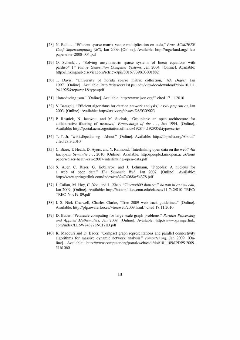
[28] N. Bell. . . , “Efficient sparse matrix-vector multiplication on cuda,” Proc. ACM/IEEEConf. Supercomputing (SC), Jan 2009. [Online]. Available: http://mgarland.org/files/papers/nvr-2008-004.pdf

[29] O. Schenk. . . , “Solving unsymmetric sparse systems of linear equations withpardiso* 1,” Future Generation Computer Systems, Jan 2004. [Online]. Available:http://linkinghub.elsevier.com/retrieve/pii/S0167739X03001882

[30] T. Davis, “University of florida sparse matrix collection,” NA Digest, Jan1997. [Online]. Available: http://citeseerx.ist.psu.edu/viewdoc/download?doi=10.1.1.94.1925&rep=rep1&type=pdf

[31] “Introducing json.” [Online]. Available: http://www.json.org/.” cited 17.11.2010

[32] V. Batagelj, “Efficient algorithms for citation network analysis,” Arxiv preprint cs, Jan2003. [Online]. Available: http://arxiv.org/abs/cs.DS/0309023

[33] P. Resnick, N. Iacovou, and M. Suchak, “Grouplens: an open architecture forcollaborative filtering of netnews,” Proceedings of the . . . , Jan 1994. [Online].Available: http://portal.acm.org/citation.cfm?id=192844.192905&type=series

[34] T. T. Jr, “wiki.dbpedia.org : About.” [Online]. Available: http://dbpedia.org/About.”cited 28.9.2010

[35] C. Bizer, T. Heath, D. Ayers, and Y. Raimond, “Interlinking open data on the web,” 4thEuropean Semantic . . . , 2010. [Online]. Available: http://people.kmi.open.ac.uk/tom/papers/bizer-heath-eswc2007-interlinking-open-data.pdf

[36] S. Auer, C. Bizer, G. Kobilarov, and J. Lehmann, “Dbpedia: A nucleus fora web of open data,” The Semantic Web, Jan 2007. [Online]. Available:http://www.springerlink.com/index/rm32474088w54378.pdf

[37] J. Callan, M. Hoy, C. Yoo, and L. Zhao, “Clueweb09 data set,” boston.lti.cs.cmu.edu,Jan 2009. [Online]. Available: http://boston.lti.cs.cmu.edu/classes/11-742/S10-TREC/TREC-Nov19-09.pdf

[38] I. S. Nick Craswell, Charles Clarke, “Trec 2009 web track guidelines.” [Online].Available: http://plg.uwaterloo.ca/~trecweb/2009.html.” cited 17.11.2010

[39] D. Bader, “Petascale computing for large-scale graph problems,” Parallel Processingand Applied Mathematics, Jan 2008. [Online]. Available: http://www.springerlink.com/index/LL6W243778N017HJ.pdf

[40] K. Madduri and D. Bader, “Compact graph representations and parallel connectivityalgorithms for massive dynamic network analysis,” computer.org, Jan 2009. [On-line]. Available: http://www.computer.org/portal/web/csdl/doi/10.1109/IPDPS.2009.5161060

III

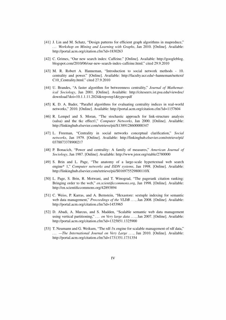
[41] J. Lin and M. Schatz, “Design patterns for efficient graph algorithms in mapreduce,”. . . Workshop on Mining and Learning with Graphs, Jan 2010. [Online]. Available:http://portal.acm.org/citation.cfm?id=1830263

[42] C. Grimes, “Our new search index: Caffeine.” [Online]. Available: http://googleblog.blogspot.com/2010/06/our-new-search-index-caffeine.html.” cited 29.9.2010

[43] M. R. Robert A. Hanneman, “Introduction to social network methods - 10.centrality and power.” [Online]. Available: http://faculty.ucr.edu/~hanneman/nettext/C10_Centrality.html.” cited 27.9.2010

[44] U. Brandes, “A faster algorithm for betweenness centrality,” Journal of Mathemat-ical Sociology, Jan 2001. [Online]. Available: http://citeseerx.ist.psu.edu/viewdoc/download?doi=10.1.1.11.2024&rep=rep1&type=pdf

[45] K. D. A. Bader, “Parallel algorithms for evaluating centrality indices in real-worldnetworks,” 2010. [Online]. Available: http://portal.acm.org/citation.cfm?id=1157604

[46] R. Lempel and S. Moran, “The stochastic approach for link-structure analysis(salsa) and the tkc effect1,” Computer Networks, Jan 2000. [Online]. Available:http://linkinghub.elsevier.com/retrieve/pii/S1389128600000347

[47] L. Freeman, “Centrality in social networks conceptual clarification,” Socialnetworks, Jan 1979. [Online]. Available: http://linkinghub.elsevier.com/retrieve/pii/0378873378900217

[48] P. Bonacich, “Power and centrality: A family of measures,” American Journal ofSociology, Jan 1987. [Online]. Available: http://www.jstor.org/stable/2780000

[49] S. Brin and L. Page, “The anatomy of a large-scale hypertextual web searchengine* 1,” Computer networks and ISDN systems, Jan 1998. [Online]. Available:http://linkinghub.elsevier.com/retrieve/pii/S016975529800110X

[50] L. Page, S. Brin, R. Motwani, and T. Winograd, “The pagerank citation ranking:Bringing order to the web,” en.scientificcommons.org, Jan 1998. [Online]. Available:http://en.scientificcommons.org/42893894

[51] C. Weiss, P. Karras, and A. Bernstein, “Hexastore: sextuple indexing for semanticweb data management,” Proceedings of the VLDB . . . , Jan 2008. [Online]. Available:http://portal.acm.org/citation.cfm?id=1453965

[52] D. Abadi, A. Marcus, and S. Madden, “Scalable semantic web data managementusing vertical partitioning,” . . . on Very large data . . . , Jan 2007. [Online]. Available:http://portal.acm.org/citation.cfm?id=1325851.1325900

[53] T. Neumann and G. Weikum, “The rdf-3x engine for scalable management of rdf data,”. . . —The International Journal on Very Large . . . , Jan 2010. [Online]. Available:http://portal.acm.org/citation.cfm?id=1731351.1731354

IV

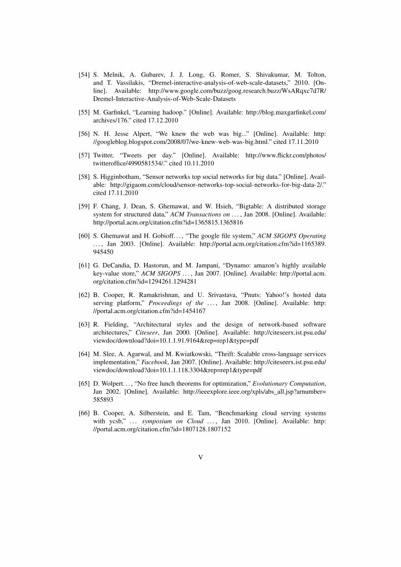
[54] S. Melnik, A. Gubarev, J. J. Long, G. Romer, S. Shivakumar, M. Tolton,and T. Vassilakis, “Dremel-interactive-analysis-of-web-scale-datasets,” 2010. [On-line]. Available: http://www.google.com/buzz/goog.research.buzz/WsARqxc7d7R/Dremel-Interactive-Analysis-of-Web-Scale-Datasets

[55] M. Garfinkel, “Learning hadoop.” [Online]. Available: http://blog.maxgarfinkel.com/archives/176.” cited 17.12.2010

[56] N. H. Jesse Alpert, “We knew the web was big...” [Online]. Available: http://googleblog.blogspot.com/2008/07/we-knew-web-was-big.html.” cited 17.11.2010

[57] Twitter, “Tweets per day.” [Online]. Available: http://www.flickr.com/photos/twitteroffice/4990581534/.” cited 10.11.2010

[58] S. Higginbotham, “Sensor networks top social networks for big data.” [Online]. Avail-able: http://gigaom.com/cloud/sensor-networks-top-social-networks-for-big-data-2/.”cited 17.11.2010

[59] F. Chang, J. Dean, S. Ghemawat, and W. Hsieh, “Bigtable: A distributed storagesystem for structured data,” ACM Transactions on . . . , Jan 2008. [Online]. Available:http://portal.acm.org/citation.cfm?id=1365815.1365816

[60] S. Ghemawat and H. Gobioff. . . , “The google file system,” ACM SIGOPS Operating. . . , Jan 2003. [Online]. Available: http://portal.acm.org/citation.cfm?id=1165389.945450

[61] G. DeCandia, D. Hastorun, and M. Jampani, “Dynamo: amazon’s highly availablekey-value store,” ACM SIGOPS . . . , Jan 2007. [Online]. Available: http://portal.acm.org/citation.cfm?id=1294261.1294281

[62] B. Cooper, R. Ramakrishnan, and U. Srivastava, “Pnuts: Yahoo!’s hosted dataserving platform,” Proceedings of the . . . , Jan 2008. [Online]. Available: http://portal.acm.org/citation.cfm?id=1454167

[63] R. Fielding, “Architectural styles and the design of network-based softwarearchitectures,” Citeseer, Jan 2000. [Online]. Available: http://citeseerx.ist.psu.edu/viewdoc/download?doi=10.1.1.91.9164&rep=rep1&type=pdf

[64] M. Slee, A. Agarwal, and M. Kwiatkowski, “Thrift: Scalable cross-language servicesimplementation,” Facebook, Jan 2007. [Online]. Available: http://citeseerx.ist.psu.edu/viewdoc/download?doi=10.1.1.118.3304&rep=rep1&type=pdf

[65] D. Wolpert. . . , “No free lunch theorems for optimization,” Evolutionary Computation,Jan 2002. [Online]. Available: http://ieeexplore.ieee.org/xpls/abs_all.jsp?arnumber=585893

[66] B. Cooper, A. Silberstein, and E. Tam, “Benchmarking cloud serving systemswith ycsb,” . . . symposium on Cloud . . . , Jan 2010. [Online]. Available: http://portal.acm.org/citation.cfm?id=1807128.1807152

V

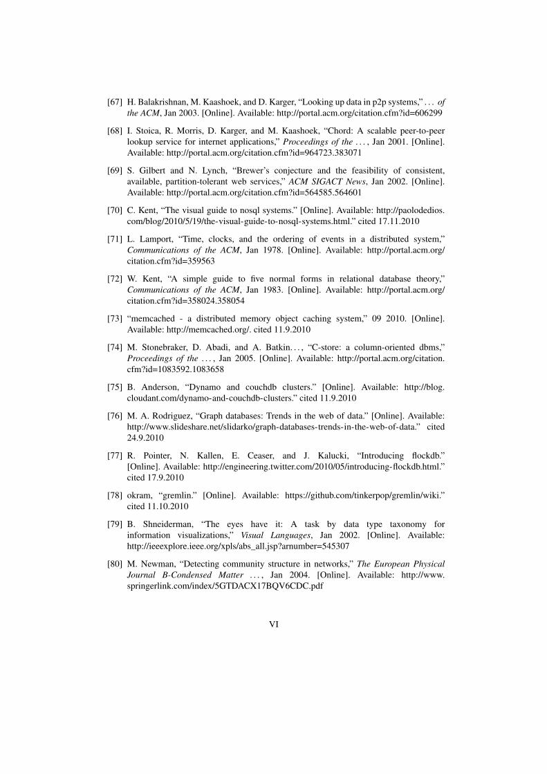
[67] H. Balakrishnan, M. Kaashoek, and D. Karger, “Looking up data in p2p systems,” . . . ofthe ACM, Jan 2003. [Online]. Available: http://portal.acm.org/citation.cfm?id=606299

[68] I. Stoica, R. Morris, D. Karger, and M. Kaashoek, “Chord: A scalable peer-to-peerlookup service for internet applications,” Proceedings of the . . . , Jan 2001. [Online].Available: http://portal.acm.org/citation.cfm?id=964723.383071

[69] S. Gilbert and N. Lynch, “Brewer’s conjecture and the feasibility of consistent,available, partition-tolerant web services,” ACM SIGACT News, Jan 2002. [Online].Available: http://portal.acm.org/citation.cfm?id=564585.564601

[70] C. Kent, “The visual guide to nosql systems.” [Online]. Available: http://paolodedios.com/blog/2010/5/19/the-visual-guide-to-nosql-systems.html.” cited 17.11.2010

[71] L. Lamport, “Time, clocks, and the ordering of events in a distributed system,”Communications of the ACM, Jan 1978. [Online]. Available: http://portal.acm.org/citation.cfm?id=359563

[72] W. Kent, “A simple guide to five normal forms in relational database theory,”Communications of the ACM, Jan 1983. [Online]. Available: http://portal.acm.org/citation.cfm?id=358024.358054

[73] “memcached - a distributed memory object caching system,” 09 2010. [Online].Available: http://memcached.org/. cited 11.9.2010

[74] M. Stonebraker, D. Abadi, and A. Batkin. . . , “C-store: a column-oriented dbms,”Proceedings of the . . . , Jan 2005. [Online]. Available: http://portal.acm.org/citation.cfm?id=1083592.1083658

[75] B. Anderson, “Dynamo and couchdb clusters.” [Online]. Available: http://blog.cloudant.com/dynamo-and-couchdb-clusters.” cited 11.9.2010

[76] M. A. Rodriguez, “Graph databases: Trends in the web of data.” [Online]. Available:http://www.slideshare.net/slidarko/graph-databases-trends-in-the-web-of-data.” cited24.9.2010

[77] R. Pointer, N. Kallen, E. Ceaser, and J. Kalucki, “Introducing flockdb.”[Online]. Available: http://engineering.twitter.com/2010/05/introducing-flockdb.html.”cited 17.9.2010

[78] okram, “gremlin.” [Online]. Available: https://github.com/tinkerpop/gremlin/wiki.”cited 11.10.2010

[79] B. Shneiderman, “The eyes have it: A task by data type taxonomy forinformation visualizations,” Visual Languages, Jan 2002. [Online]. Available:http://ieeexplore.ieee.org/xpls/abs_all.jsp?arnumber=545307

[80] M. Newman, “Detecting community structure in networks,” The European PhysicalJournal B-Condensed Matter . . . , Jan 2004. [Online]. Available: http://www.springerlink.com/index/5GTDACX17BQV6CDC.pdf

VI

[81] K. Madduri, D. Bader, J. Berry, and J. Crobak, “Parallel shortest path algo-rithms for solving large-scale instances,” 9th DIMACS Implementation . . . , Jan2006. [Online]. Available: http://citeseerx.ist.psu.edu/viewdoc/download?doi=10.1.1.106.7020&rep=rep1&type=pdf

[82] L. Freeman, “Visualizing social networks,” Journal of social structure, Jan2000. [Online]. Available: http://citeseerx.ist.psu.edu/viewdoc/download?doi=10.1.1.87.6279&rep=rep1&type=pdf

[83] D. Holten and J. van Wijk, “Force-directed edge bundling for graph visualization,”Computer Graphics Forum, Jan 2009. [Online]. Available: http://www3.interscience.wiley.com/journal/122523375/abstract

[84] P. Butler, “Visualizing friendships.” [Online]. Available: http://www.facebook.com/note.php?note_id=469716398919.” cited 17.12.2010

[85] J. E. et al, “Graphviz - graph visualization software.” [Online]. Available:http://www.graphviz.org/.” cited 6.12.2010

[86] A. Barabási. . . , “Emergence of scaling in random networks,” Science, Jan 1999.[Online]. Available: http://www.sciencemag.org/cgi/content/abstract/sci;286/5439/509

[87] T. Haveliwala, “Efficient computation of pagerank,” Citeseer, Jan 1999.[Online]. Available: http://citeseerx.ist.psu.edu/viewdoc/download?doi=10.1.1.65.3145&rep=rep1&type=pdf

[88] K. Haugen, “Analysis of the nosql landscape.” [Online]. Available: http://blog.knuthaugen.no/2010/03/the-nosql-landscape.html.” cited 22.11.2010

[89] M. P. Sean Cribbs, “Riak: An open source internet-scale data store.” [Online].Available: http://wiki.basho.com/.” cited 11.9.2010

[90] D. S. Justin Sheehy, “Bitcask. a log-structured hash table for fast key/value data,” 042010. [Online]. Available: http://downloads.basho.com/papers/bitcask-intro.pdf. cited27.4.2010

[91] M. Raynal and M. Singhal, “Logical time: Capturing causality in distributed systems,”Computer, Jan 1996. [Online]. Available: http://ieeexplore.ieee.org/xpls/abs_all.jsp?arnumber=485846

[92] S. Metson, “Cern: A case study.” [Online]. Available: http://www.couch.io/case-study-cern.” cited 11.10.2010

[93] S. Maniyam, “Hbase: Bigtable-like structured storage for hadoop hdfs.” [Online].Available: http://wiki.apache.org/hadoop/Hbase.” cited 13.10.2010

[94] D. Carstoiu, A. Cernian, and A. Olteanu, “Hadoop hbase-0.20. 2 performanceevaluation,” New Trends in Information . . . , Jan 2010. [Online]. Available:http://ieeexplore.ieee.org/xpls/abs_all.jsp?arnumber=5488644

VII

[95] A. Khetrapal and V. Ganesh, “Hbase and hypertable for large scale distributedstorage systems,” Dept. of Computer Science, 2010. [Online]. Available: http://www.uavindia.com/ankur/downloads/HypertableHBaseEval2.pdf

[96] K. Madduri, “Snap, small-world network analysis and partitioning: An open-source parallel graph framework for the exploration of large-scale networks,”Parallel and Distributed Processing, pp. 1–12, Jan 2008. [Online]. Available:http://ieeexplore.ieee.org/xpls/abs_all.jsp?arnumber=4536261

[97] A. Hotho, R. Jäschke, and C. Schmitz. . . , “Information retrieval in folksonomies:Search and ranking,” The Semantic Web: . . . , Jan 2006. [Online]. Available:http://www.springerlink.com/index/r8313654k80v7231.pdf

[98] E. Gansner and Y. Koren. . . , “Graph drawing by stress majorization,”Graph Drawing, Jan 2005. [Online]. Available: http://www.springerlink.com/index/JRN52J7CX8GRCY6V.pdf

[99] T. Hoff, “Building super scalable systems: Blade runner meets autonomic computingin the ambient cloud.” [Online]. Available: http://highscalability.com/blog/2009/12/16/building-super-scalable-systems-blade-runner-meets-autonomic.html.” cited28.9.2010

[100] D. Anderson, J. Cobb, and E. Korpela. . . , “Seti@ home: an experiment inpublic-resource computing,” . . . of the ACM, Jan 2002. [Online]. Available:http://portal.acm.org/citation.cfm?id=581571.581573

[101] A. Dou, V. Kalogeraki, and D. Gunopulos, “Misco: a mapreduce frameworkfor mobile systems,” Proceedings of the . . . , Jan 2010. [Online]. Available:http://portal.acm.org/citation.cfm?id=1839294.1839332

VIII