stochastic calculus: applications in finance - christophe chorro

1

Stochastic Calculus:

Applications in Finance

Master M2 IRFA, QEM 2

Christophe Chorro

September 2009

(If you see some misprints or errors please contact me at [email protected] !!!)

0.0 0.1 0.2 0.3 0.4 0.5 0.6 0.7 0.8 0.9 1.0 1.1!140

!120

!100

!80

!60

!40

!20

0

20

Contents

0.1 Introduction . . . . . . . . . . . . . . . . . . . . . . . . . . . . . . 70.1.1 Definition . . . . . . . . . . . . . . . . . . . . . . . . . . . 7

0.2 Notion of independence . . . . . . . . . . . . . . . . . . . . . . . . 80.2.1 Events . . . . . . . . . . . . . . . . . . . . . . . . . . . . . 80.2.2 σ-algebras . . . . . . . . . . . . . . . . . . . . . . . . . . 90.2.3 Random variables . . . . . . . . . . . . . . . . . . . . . . . 90.2.4 Convergence of random variables . . . . . . . . . . . . . . 10

0.3 Gaussian vectors . . . . . . . . . . . . . . . . . . . . . . . . . . . 150.4 Conditional expectation . . . . . . . . . . . . . . . . . . . . . . . 16

0.4.1 Conditioning with respect to events . . . . . . . . . . . . . 160.4.2 Conditioning with respect to discrete random variables . . 160.4.3 Conditioning with respect to σ-algebras . . . . . . . . . . . 160.4.4 Conditioning with respect to general random variables . . 170.4.5 Conditional distribution . . . . . . . . . . . . . . . . . . . 170.4.6 Properties of conditional expectation . . . . . . . . . . . . 180.4.7 Conditional expectation and Gaussian vectors . . . . . . . 20

0.5 Stochastic processes . . . . . . . . . . . . . . . . . . . . . . . . . . 200.5.1 Introduction . . . . . . . . . . . . . . . . . . . . . . . . . . 200.5.2 Filtrations, adapted processes . . . . . . . . . . . . . . . . 230.5.3 Gaussian processes . . . . . . . . . . . . . . . . . . . . . . 250.5.4 Martingales in continuous time . . . . . . . . . . . . . . . 26

0.6 Radon-Nikodym’s theorem . . . . . . . . . . . . . . . . . . . . . 27Bibliography . . . . . . . . . . . . . . . . . . . . . . . . . . . . . . . . 31

1 Brownian motion 331.1 Short history . . . . . . . . . . . . . . . . . . . . . . . . . . . . . 331.2 Definition, existence, simulation . . . . . . . . . . . . . . . . . . . 36

1.2.1 Definition . . . . . . . . . . . . . . . . . . . . . . . . . . . 361.2.2 Existence, construction, simulation . . . . . . . . . . . . . 37

1.3 Properties . . . . . . . . . . . . . . . . . . . . . . . . . . . . . . . 411.3.1 Martingale property . . . . . . . . . . . . . . . . . . . . . 411.3.2 Transformations . . . . . . . . . . . . . . . . . . . . . . . . 411.3.3 Regularity of the paths . . . . . . . . . . . . . . . . . . . . 42

3

4 CONTENTS

1.3.4 Variation and quadratic variation . . . . . . . . . . . . . . 431.3.5 Markov property . . . . . . . . . . . . . . . . . . . . . . . 451.3.6 Geometric Brownian motion . . . . . . . . . . . . . . . . . 451.3.7 Wiener Integral . . . . . . . . . . . . . . . . . . . . . . . . 461.3.8 Ito formula for B.M . . . . . . . . . . . . . . . . . . . . . . 501.3.9 Applications of the Wiener integral . . . . . . . . . . . . . 53

2 Stochastic integral, Ito processes. 612.1 The stochastic integral on E([0, T ]× Ω) . . . . . . . . . . . . . . . 61

2.1.1 Definition . . . . . . . . . . . . . . . . . . . . . . . . . . . 612.1.2 Properties of the Ito integral of an elementary process . . . 62

2.2 Extension to L2prog(Ω× [0, T ]) . . . . . . . . . . . . . . . . . . . . 63

2.3 Ito Process . . . . . . . . . . . . . . . . . . . . . . . . . . . . . . . 652.4 Extended Ito Calculus . . . . . . . . . . . . . . . . . . . . . . . . 672.5 Stochastic differential equations (SDE) . . . . . . . . . . . . . . . 69

2.5.1 Geometric Brownian motion . . . . . . . . . . . . . . . . . 692.5.2 General case . . . . . . . . . . . . . . . . . . . . . . . . . . 712.5.3 The Markov property of solutions . . . . . . . . . . . . . . 732.5.4 Simulation of solutions of S.D.E (a first step) . . . . . . . 74

3 Two fundamental results 773.1 Girsanov’s theorem . . . . . . . . . . . . . . . . . . . . . . . . . . 773.2 Martingale representation theorem . . . . . . . . . . . . . . . . . 79Bibliography . . . . . . . . . . . . . . . . . . . . . . . . . . . . . . . . 83

4 Applications to finance (general framework) 854.1 Introduction . . . . . . . . . . . . . . . . . . . . . . . . . . . . . . 85

4.1.1 Some historical aspects . . . . . . . . . . . . . . . . . . . . 854.1.2 Stochastic integral? . . . . . . . . . . . . . . . . . . . . . . 864.1.3 Is the stochastic calculus a new invisible hand? . . . . . . 87

4.2 Modelling financial markets in continuous time . . . . . . . . . . . 884.2.1 Description of financial assets . . . . . . . . . . . . . . . . 884.2.2 Financial strategies . . . . . . . . . . . . . . . . . . . . . . 884.2.3 Self-financing condition . . . . . . . . . . . . . . . . . . . . 894.2.4 Arbitrages . . . . . . . . . . . . . . . . . . . . . . . . . . . 904.2.5 Equivalent martingale measures (E.M.E) . . . . . . . . . . 914.2.6 Contingent claims . . . . . . . . . . . . . . . . . . . . . . . 92

4.3 Study plan and objectives . . . . . . . . . . . . . . . . . . . . . . 92

5 The Black-Scholes model 975.1 The model . . . . . . . . . . . . . . . . . . . . . . . . . . . . . . . 97

5.1.1 Dynamic of the risky asset . . . . . . . . . . . . . . . . . 97

CONTENTS 5

5.1.2 Existence of an EMM . . . . . . . . . . . . . . . . . . . . . 985.2 P ∗ admissible financial strategies . . . . . . . . . . . . . . . . . . 98

5.2.1 Definition . . . . . . . . . . . . . . . . . . . . . . . . . . . 995.2.2 P ∗-completeness of the market . . . . . . . . . . . . . . . 995.2.3 N.A.O among P ∗ admissible strategies . . . . . . . . . . . 100

5.3 Unicity of the risk neutral probability . . . . . . . . . . . . . . . . 1015.4 Pricing, Hedging . . . . . . . . . . . . . . . . . . . . . . . . . . . 1015.5 Pricing and Hedging when h = f(ST ) . . . . . . . . . . . . . . . . 1025.6 Black and Scholes formula . . . . . . . . . . . . . . . . . . . . . . 1045.7 The greeks . . . . . . . . . . . . . . . . . . . . . . . . . . . . . . . 106

5.7.1 Definition . . . . . . . . . . . . . . . . . . . . . . . . . . . 1065.7.2 Payoff of the form h = f(ST ) . . . . . . . . . . . . . . . . 1075.7.3 Practical use of ∆ and Γ . . . . . . . . . . . . . . . . . . . 109

5.8 Black and Scholes in practice . . . . . . . . . . . . . . . . . . . . 1095.8.1 Estimating volatility σ . . . . . . . . . . . . . . . . . . . . 1095.8.2 Pricing and Hedging . . . . . . . . . . . . . . . . . . . . . 1105.8.3 Numerical computations of prices, of ∆ and of Γ . . . . . . 111

5.9 “Splendeurs et miseres“ of the Black Scholes model . . . . . . . . 1165.9.1 Advantages . . . . . . . . . . . . . . . . . . . . . . . . . . 1165.9.2 Limites . . . . . . . . . . . . . . . . . . . . . . . . . . . . . 118

6 CONTENTS

Reminder on Probability theory

This chapter is not an elementary introduction to Probability theory. Here wejust remind some fundamental results that will be used in the sequel. For moredetails we refer the reader to [1] and [2].

∀d ∈ N∗, let us denote by B(Rd) the borelian σ-algebra on Rd, <,> the usualscalar product on Rd and dx the Lebesgue measure on Rd.

0.1 Introduction

0.1.1 Definition

Let (Ω,A, P ) be a probability space.

Definition 0.1.1 A random variable is a function X : (Ω,A, P ) → Rd such that∀E ∈ B(Rd), X−1(E) ∈ A.

Remark 0.1.1 a) There exists a natural σ-algebra on Ω in order for X to bemeasurable. This σ-algebra is defined by σ(X) = X−1(E);E ∈ B(Rd) and isthe smallest in the inclusion sense. We can show (exercise) that each randomvariable measurable with respect to σ(X) has the form h(X) where h is borelian.b) The notion of measurability is preserved by elementary algebraic operations andby passing to the limit. When Ω is a topological space equipped with its borelianσ-algebra, the continuity implies the measurability.

Definition 0.1.2 For A ⊂ Ω, 1A is defined to be the function fulfilling 1A(x) = 1if x ∈ A and 1A(x) = 0 if x ∈ Ac. If A ∈ A, 1A is measurable and in this caseσ(A) = Ω, ∅, A,Ac.

Random variables allow to transport probabilistic structures:

Proposition 0.1.1 If X : (Ω,A, P ) → Rd is a random variable, the mappingPX : B(Rd) → R+ defined, ∀E ∈ B(Rd), by PX(E) = P (X−1(E)) is a probabilitymeasure on (Rd,B(Rd)) called the distribution of X.

7

8 CONTENTS

Definition 0.1.3 We say that a random variable X has a moment of order p ∈N∗ if the quantity

E[|X|p] =

∫Rd

|x|pdPX(x)

is finite. For p ∈ N∗, we define Lp = X;E[|X|p] < ∞ and if X ∈ Lp,

‖ X ‖p= E[|X|p]1p . Remember that (Lp, ‖ X ‖p) is complete (because every sum

that absolutely converges is convergent...).

Example 0.1.1 When d = 1, we say that X follows a gaussian distribution ofmean m and variance σ2 (the standard notation is N (m,σ2)) if PX is absolutelycontinuous with respect to dx and if

dPX(x) =1√

2πσ2e−

(x−m)2

2σ2 dx.

In this case, X has moments of all orders, in particular, E[X] = m and V ar(X) =E[(X − E[X])2] = σ2.

Exercise 0.1.1 Let X be a random variable following a N (0, σ2). Show that∀k ∈ N,

E[X2k] =(2k)!

2kk!σ2k.

An useful characterization of probability distributions is given by the followingtheorem:

Theorem 0.1.1 a) The characteristic function ΦX : t ∈ Rd → E[ei<t,X>] ∈ Ccharacterize the distribution of X.b) If d = 1, the distribution of X is characterized by the distribution functionFX : t ∈ R → P (X ≤ t) ∈ R+.

Example 0.1.2 If X follows a N (m,σ2), then

ΦX(t) = eitme−σ2t2

2 .

0.2 Notion of independence

0.2.1 Events

Definition 0.2.1 Two events A and B (in A) are independent if P (A ∩ B) =P (A)P (B). In this case, we use the classical notation A⊥B (This notation willremain valid for σ-algebras and random variables).

0.2. NOTION OF INDEPENDENCE 9

Definition 0.2.2 A finite collection of events (Ai)1≤i≤n is an independent col-lection if P (∩i∈IAi) =

∏i∈IP (Ai), ∀I ⊂ 1, ..., n. Often, the events are said to be

mutually independent.

Remark 0.2.1 Warning: If events are pairwise independent they are not mutu-ally independent in general. In fact, considering the toss of two fair coins we canshow that the events

A=“head on first coin”B=“tail on second coin”C=“The same on the two coins”

are pairwise but not mutually independent.

0.2.2 σ-algebras

Definition 0.2.3 Sub σ-algebras (Ai)1≤i≤n of A are independent if one has P (∩1≤i≤nAi) =∏1≤i≤n

P (Ai), ∀Ai ∈ Ai.

0.2.3 Random variables

Definition 0.2.4 Random variables (Xi)1≤i≤n are independent if the generatedσ-algebras (σ(Xi))1≤i≤n are independent .

We consider for notational simplicity that d = 1. However the results extendwithout difficulty to the general case.

Theorem 0.2.1 : In order for X1 and X2 to be independent, it is necessary andsufficient to have any one of the following conditions holdinga) P(X1,X2) = PX1 ⊗ PX2

b) ∀f, g ∈ Cb(R,R), E[f(X1)g(X2)] = E[f(X1)]E[g(X2)]c) Φ(X1,X2) = ΦX1ΦX2

Proposition 0.2.1 If X1 et X2 are independent one has V ar(X1+X2) = V ar(X1)+V ar(X2) and E[X1X2] = E[X1]E[X2]. The last equality implies that two inde-pendent random variables are uncorrelated, unfortunately the converse is false ingeneral ( take X1 = X, X2 = X2 with X symmetric). For more details, thereader can read the forthcoming part on gaussian vectors.

Proposition 0.2.2 If X1 et X2 are two random variables so that the pair (X1, X2)owns a density, then, X1 and X2 are independent if and only if the density of thepair is equal to the product of the densities of each component.

10 CONTENTS

Exercise 0.2.1 (Box-Muller Method) Consider that U1 and U2 are two indepen-dent uniform random variables on the interval [0, 1]. Show that

G1 =√−2log(U1)cos(2πU2) and G2 =

√−2log(U1)sin(2πU2)

are two independent N (0, 1).

Proof: Let us write

Φ : (x, y) ∈]0, 1[2→ (u =√−2log(x)cos(2πy), v =

√−2log(x)sin(2πy)) ∈ R2−(R+×0).

It is easy to prove that Φ is a C1-diffeomorphism with a Jacobian determinantfulfilling |J(Φ)(x, y)| = 2π

x. Since u2 + v2 = −2log(x) thus |J(Φ−1)(u, v)| =

12πe−

u2+v2

2 .According to the change of variables theorem, one has for F ∈ Cb(R2,R),∫]0,1[2

F (Φ(x, y))dxdy =

∫R2−(R+×0)

F (u, v)1

2πe−

u2+v2

2 dudv.2

0.2.4 Convergence of random variables

Types of convergence

For simplicity we assume that d = 1.

Lemma 0.2.1 (Borel-Cantelli) Let (An)N∗ be a sequence of events in A.

a) If+∞∑n=1

P (An) <∞, then

P (ω ∈ Ω;ω ∈ An for an infinite number of n) = 0.

b) If the An’s are mutually independent with+∞∑n=1

P (An) = +∞, then,

P (ω ∈ Ω;ω ∈ An for an infinite number of n) = 1.

Definition 0.2.5 We say that a sequence of random variables (Xn)n≥0convergestoward X almost surely (Xn →

a.sX) if

P (ω ∈ Ω;Xn(ω) →n→∞

X(ω)) = 1.

Proposition 0.2.3 Using B.C, we can show that Xn →a.sX if ∀ε > 0,

+∞∑n=1

P (|Xn −X| > ε) <∞.


Lemma 0.2.2 Classical inequalities:

a) (Tchebychev) If X ∈ Lp, λ > 0,

P (|X| > λ) ≤ 1

λpE[|X|p].

b) (Holder) If X ∈ Lp, Y ∈ Lq with 1p

+ 1q

= 1, then (by concavity of the log

ab ≤ ap

p+ bq

q...),

E[|XY |] ≤‖ X ‖p + ‖ Y ‖q .

c) (Minkowsky) If X ∈ Lp, Y ∈ Lp (by convexity of xp)

‖ X + Y ‖p≤‖ X ‖p‖ Y ‖p .

Definition 0.2.6 If (Xn)n>0 et X have finite moments of order p ∈ N∗, we saythat (Xn)n>0 converges in Lp toward X (Xn →

LpX) if

E[|Xn −X|p] →n→∞

0.

Definition 0.2.7 We say that a sequence of random variables (Xn)n>0 convergestoward X in probability (Xn →

pX) if ∀ε > 0

P (|X −Xn| > ε) →n→∞

0.

Definition 0.2.8 We say that a sequence of random variables (Xn)n>0 convergestoward X in distribution ( Xn →

DX) if ∀f ∈ Cb(R,R),

E[f(Xn] →n→∞

E[f(X)].

Proposition 0.2.4 The following propositions are equivalent.a) Xn →

DX

b) FXn converges pointwise to FX for all point in the set of continuity of FX(d = 1)c) ΦXn converges pointwise to ΦX

Exercise 0.2.2 Let (Gn) be a sequence of Gaussian random variables that con-verges toward G in L2. Show that G is Gaussian.

12 CONTENTS

Relation between the different types of convergence

Proposition 0.2.5 a) Xn →a.sX ⇒ Xn →

pX

b) Xn →L1X ⇒ Xn →

pX

c) Xn →pX ⇒ Xn →

DX

d) Si q ≥ p, Xn →LqX ⇒ Xn →

LpX

Proof a) comes from proposition 0.2.3.b) Direct consequence of Tchebychev inequality.c) Let f ∈ Cb(R,R) and ε > 0,

|E[f(Xn)]−E[f(X)]| ≤ E[|f(Xn)−f(X)|1|Xn−X|>ε]+E[|f(Xn)−f(X)|1|Xn−X|≤ε].

One has E[|f(Xn) − f(X)|1|Xn−X|>ε] ≤ cstP (|Xn − X| > ε) →n→∞

0. Consider

g ∈ CK(R,R) so that ‖ f − g ‖∞≤ ε,

E[|f(Xn)− f(X)|1|Xn−X|≤ε] ≤ 2ε+ E[|g(Xn)− g(X)|1|Xn−X|≤ε].

The function g being uniformly continuous, ∃η > 0 such that

|x− y| ≤ η ⇒ |g(x)− g(y)| ≤ ε,

thus,

E[|g(Xn)− g(X)|1|Xn−X|≤ε] ≤ ε+ cstP (|Xn −X| ≥ η)

with P (|Xn −X| ≥ η) →n→∞

0.

d) Direct consequence of Holder inequality. 2

Remark 0.2.2 a) All the other implications are false in general.b) The a.s convergence is the only type that allows the usual algebraic stabil-ity. Thus, a good way to overcome mistakes is to come back to the definitions.(counter-example: Xn = −X where X is symmetric, Xn converges in distributiontoward X and Xn −X converges in distribution toward −2X...).

The following results give partial converses to proposition 0.2.5.

Definition 0.2.9 A family Xi; i ∈ I of random variables in L1 is said to beuniformly integrable (U.I) if

supi∈I

E[|Xi|1|Xi|>n] →n→∞

0.


Example 0.2.1 a) If I is finite Xi; i ∈ I is U.I.

b) if ∃Y ∈ L1 such that ∀i ∈ I |Xi| ≤ Y , Xi; i ∈ I is U.I.

Theorem 0.2.2 If Xn →pX and if the sequence (Xn) is U.I, then, X ∈ L1 and

Xn →L1X.

The following result is a direct consequence of proposition 0.2.3.

Theorem 0.2.3 If Xn →pX, then there exists an extraction φ such that Xφ(n) →

a.s

X.

Theorem 0.2.4 If Xn →Dc, where c is a constant then Xn →

pc.

Two important results

Theorem 0.2.5 (SLLN) Let (Xn) be a sequence of i.i.d random variables.

a) Suppose that X ∈ L1. Denoting Sn = X1 + ...+Xn, one has

Snn

→a.s and L1

E[X1].

b) If E[|X1|] = +∞ the sequence Sn diverges a.s.

0 50 100 150 200 250 300 350 400 450 5000.0

0.1

0.2

0.3

0.4

0.5

0.6

Illustration of the SLLN when X1 → B(12) and n = 500

14 CONTENTS

0 1000 2000 3000 4000 5000 6000 7000 8000 9000 10000!25

!20

!15

!10

!5

0

5

10

SLLN is not fulfilled when X1 → C(1) (here n = 10000)

The central limit theorem gives some precisions concerning the speed of con-vergence in the strong law of large numbers:

Theorem 0.2.6 (CLT) Let (Xn) be a sequence of i.i.d random variables. Sup-pose that X1 has finite moment of order 2 and put m = E[X1] and σ2 = V ar(X1).One obtains

Sn−nm√nσ

→DN (0, 1).

!! !" !# $ # " !$%$$

$%$&

$%#$

$%#&

$%"$

$%"&

$%!$

$%!&

$%'$

$%'&

Illustration of the CLT when X1 → U([0, 1]) and n = 500

0.3. GAUSSIAN VECTORS 15

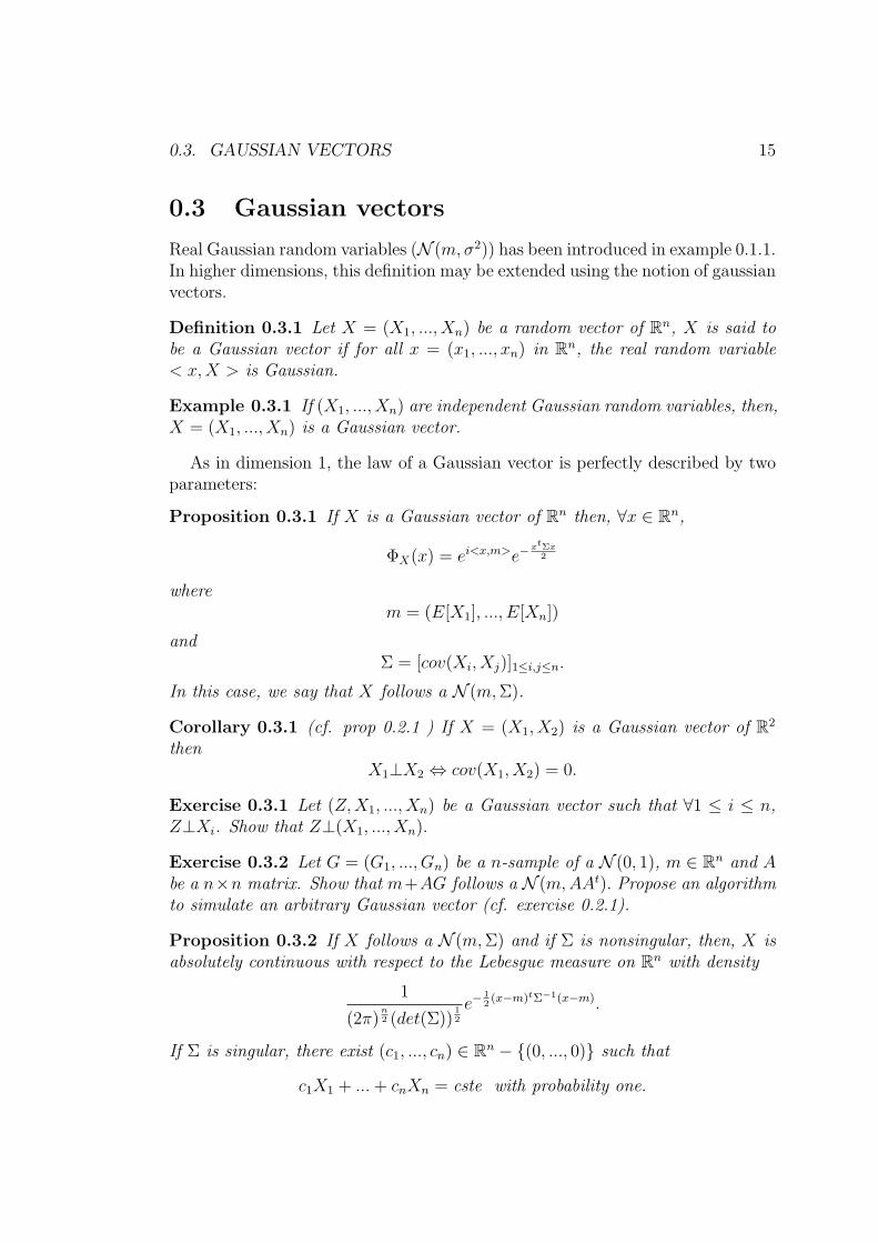
0.3 Gaussian vectors

Real Gaussian random variables (N (m,σ2)) has been introduced in example 0.1.1.In higher dimensions, this definition may be extended using the notion of gaussianvectors.

Definition 0.3.1 Let X = (X1, ..., Xn) be a random vector of Rn, X is said tobe a Gaussian vector if for all x = (x1, ..., xn) in Rn, the real random variable< x,X > is Gaussian.

Example 0.3.1 If (X1, ..., Xn) are independent Gaussian random variables, then,X = (X1, ..., Xn) is a Gaussian vector.

As in dimension 1, the law of a Gaussian vector is perfectly described by twoparameters:

Proposition 0.3.1 If X is a Gaussian vector of Rn then, ∀x ∈ Rn,

ΦX(x) = ei<x,m>e−xtΣx

2

wherem = (E[X1], ..., E[Xn])

andΣ = [cov(Xi, Xj)]1≤i,j≤n.

In this case, we say that X follows a N (m,Σ).

Corollary 0.3.1 (cf. prop 0.2.1 ) If X = (X1, X2) is a Gaussian vector of R2

thenX1⊥X2 ⇔ cov(X1, X2) = 0.

Exercise 0.3.1 Let (Z,X1, ..., Xn) be a Gaussian vector such that ∀1 ≤ i ≤ n,Z⊥Xi. Show that Z⊥(X1, ..., Xn).

Exercise 0.3.2 Let G = (G1, ..., Gn) be a n-sample of a N (0, 1), m ∈ Rn and Abe a n×n matrix. Show that m+AG follows a N (m,AAt). Propose an algorithmto simulate an arbitrary Gaussian vector (cf. exercise 0.2.1).

Proposition 0.3.2 If X follows a N (m,Σ) and if Σ is nonsingular, then, X isabsolutely continuous with respect to the Lebesgue measure on Rn with density

1

(2π)n2 (det(Σ))

12

e−12(x−m)tΣ−1(x−m).

If Σ is singular, there exist (c1, ..., cn) ∈ Rn − (0, ..., 0) such that

c1X1 + ...+ cnXn = cste with probability one.

16 CONTENTS

0.4 Conditional expectation

Let X and Y be two random variables taking values in R. It often arises thatwe already know the value of X and want to calculate the expected value of Ytaking into account this knowledge. This is the intuitive meaning of conditionalexpectation.

0.4.1 Conditioning with respect to events

Let A and B be in A with P (B) > 0. We define

P (A|B) =:P (A ∩B)

P (B).

In the same way, if X ∈ L1, we define

E[X|B] =:E[X1B]

P (B).

0.4.2 Conditioning with respect to discrete random vari-ables

Let Y be a discrete random variable taking values D = y1, ....yn, ... and supposethat ∀y ∈ D, P (Y = y) > 0.

If A belongs to A, one defines

P (A|Y ) =: φ(Y ) where ∀y ∈ D, φ(y) = P (A|Y = y).

Similarly, if X ∈ L1, one defines

E[X|Y ] =: ψ(Y ) where ∀y ∈ D,ψ(y) = E[X|Y = y].

It is very important to notice that P (A|Y ) and E[X|Y ] are random variables.

Remark 0.4.1 : When Y is a continuous random variable, the preceding defi-nition is meaningless because ∀y ∈ R, P (Y = y) = 0. We have to adopt anotherpoint of view.

0.4.3 Conditioning with respect to σ-algebras

Let (Ω,A, P ) be a probability space, X a random variable in L1 and G a subσ-algebra of A.

0.4. CONDITIONAL EXPECTATION 17

Definition 0.4.1 (Theorem) There exists a random variable Z ∈ L1 such that

i) Z is G-measurable

ii) E[XU ] = E[ZU ] ∀U G-measurable and bounded.

Z is denoted by E[X|G] and is called the conditional expectation of X given G.Moreover, Z is unique up to a.s equality.

Remark 0.4.2 : The preceding result is based on the powerful Radon Nikodymtheorem (paragraph 0.6). Nevertheless, when X ∈ L2, the existence of Z can beproved using Hilbert space methods. If fact, considering the orthogonal projectionΠ of L2(Ω,A, P ) on the closed convex set L2(Ω,G, P ) we show easily that Π(X) =E[X|G]. Intuitively, E[X|G] is the best approximation of X by G-measurablerandom variables.

0.4.4 Conditioning with respect to general random vari-ables

Let Y be a random variable.

Definition 0.4.2 When X ∈ L1, E[X|Y ] is defined to be E[X|σ(Y )].

According to remark 0.1.1, E[X|Y ] is of the form ψ(Y ) where ψ : R → R isborelian. Naturally, this definition coincides with the one proposed in paragraph0.4.2 in the discrete case.

Remark 0.4.3 Using remark 0.1.1, the preceding definition may be rewritten inthe following way

i) E[X|Y ] is σ(Y )-measurable

ii) E[Xg(Y )] = E[E[X|Y ]g(Y )] ∀g borelian and bounded.

0.4.5 Conditional distribution

Let us consider a pair (X, Y ) of real random variables in L1. Suppose that thispair owns a density f(X,Y ) with respect to the Lebesgue measure on R2. Thus,the marginal densities of X and Y are given by

fX(x) =

∫Rf(X,Y )(x, y)dy and fY (y) =

∫Rf(X,Y )(x, y)dx.

When X⊥Y , one has f(X,Y ) = fXfY . If the condition of independence is re-laxed, we obtain the following disintegration formula : f(X,Y )(x, y) = fX|Y (x, y)fY (y)where

fX|Y (x, y) =f(X,Y )(x, y)

fY (y)

18 CONTENTS

if fY (y) 6= 0 and fX|Y (x, y) = 0 otherwise. The function fX|Y is called theconditional density of X given Y . In fact, if φ satisfies φ(X) ∈ L1,

E[φ(X)|Y ] = Φ(Y ) with Φ(y) =

∫Rφ(x)fX|Y (x, y)dx.

0.4.6 Properties of conditional expectation

Classical properties of expectation

Proposition 0.4.1 Let X and Y be two random variables in L1 and G a subσ-algebra of A.

a) (positivity) If X ≥ 0 P -a.s, E[X|G] ≥ 0 P -a.s.

b) (linearity) If (α, β) ∈ R2, E[αX + βY |G] = αE[X|G] + βE[Y |G] P -a.s.

c) (monotony) If X ≥ Y P -a.s, E[X|G] ≥ E[Y |G] P -a.s. (Consider E[Y |G]−E[X|G] ≥ ε.)

d) (Beppo-levy) If Xn is a sequence of non negative random variables in L1

with Xn ↑ X P -a.s, then E[Xn|G] ↑ E[X|G] P -a.s.

e) (Fatou) If Xn is a sequence of non negative random variables in L1, thenE[lim inf

nXn|G] ≤ lim inf

nE[Xn|G] P -a.s.

f) (Dominated convergence) If Xn is a sequence of random variables in L1 suchthat Xn →

a.sX and ∀n ∈ N, Xn ≤ X ∈ L1, then, E[Xn|G] →

a.s and L1

E[X|G].

g) (Jensen) If ψ : R → R is a convex function such that ψ(X) ∈ L1, then,ψ(E[X|G]) ≤ E[ψ(X)|G] P -a.s.

Remark 0.4.4 We deduce from g) that the conditional expectation is a contract-ing operator on Lp spaces.

Specific properties

Proposition 0.4.2 Let X and Y be two random variables in L1 and G a subσ-algebra of A.

a) E[E[X|G]] = E[X]

b) If X is G-measurable, E[X|G] = X P -a.s.

0.4. CONDITIONAL EXPECTATION 19

c) (Taking out what is known) If Y is G-measurable and bounded, E[XY |G] =Y E[X|G] P -a.s.

d) (Role of independence) If σ(X)⊥G, E[X|G] = E[X] P -a.s.

e) (Tower property) If G ′ is a sub σ-algebra of A such that G ′ ⊂ G, then,E[E[X|G]|G ′] = E[X|G ′] P -a.s.

f) If (Gi)i∈I is a collection of sub σ-algebras of A, the family (E[X|Gi])i∈I isU.I.

Proof: We only give the proof of f), the others are left to the reader. Accordingto Jensen inequality for conditional expectation,

E[|E[X|Gi]|1|E[X|Gi]|>n] ≤ E[E[|X| |Gi]1|E[X|Gi]|>n] = E[|X|1|E[X|Gi]|>n].

But, from Tchebychev inequality one obtains

P (|E[X|Gi]| > n) ≤ E[|E[X|Gi]|]n

≤ E[E[|X| |Gi]]n

=E[|X|]n

.

We conclude using the following lemma:

Lemma 0.4.1 Si X ∈ L1, ∀ε > 0, ∃δ > 0, P (A) < δ ⇒ E[|X|1A] < ε.

2

The preceding properties are often sufficient to compute conditional expecta-tions. We only come back to the definition for more difficult cases as we can seein the following proposition.

The following result will be useful in the study of the Black-Scholes model andmore generally to prove Markov properties of stochastic processes.

Proposition 0.4.3 If σ(X)⊥G and if Y is G-measurable, then, for all borelianfunction Φ : R2 → R such that E[|Φ(X, Y )|] <∞, one has

E[Φ(X, Y )|G] = ψ(Y ) where ψ(y) = E[Φ(X, y)].

Proof: We have ψ(y) =∫

R Φ(x, y)dPX(x) and the measurability of ψ is aclassical consequence of Fubini’s theorem. For G ∈ G, we set Z = 1G. We deducefrom the hypotheses that P(X,Y,Z) = PX ⊗ P(Y,Z), thus,

E[Φ(X, Y )1G] =

∫R

∫R2

Φ(x, y)zdP(Y,Z)(y, z)dPX(x).

20 CONTENTS

By Fubini’s theorem,

E[Φ(X, Y )1G] =

∫R2

ψ(y)zdP(Y,Z)(y, z)

soE[Φ(X, Y )1G] = E[ψ(Y )1G].

2

0.4.7 Conditional expectation and Gaussian vectors

Proposition 0.4.4 Let (Z,X1, ..., Xn) be a Gaussian vector. Then, there existreal numbers (a, b1, ..., bn) such that

E[Z|X1, ..., Xn] = a+n∑i=1

Xibi.

Proof: Consider the closed sub vector space (of finite dimension) of L2 spannedby (1, X1, ..., Xn). Let Π denotes the orthogonal projection on this closed and con-

vex set. Thus, there exist real numbers (a, b1, ..., bn) such that Π(Z) = a+n∑i=1

Xibi.

For Y = Z − Π(Z), one obtains classically E[Y ] = 0 and E[Y Xi] = 0. In thisway, cov(Y,Xi) = 0. The random vector (Y,Xi) being Gaussian, we deduce fromcorollary 0.3.1, Y⊥Xi. By exercise 0.3.1, Y⊥(X1, ..., Xn) and E[Y |X1, ..., Xn] =

E[Y ] = 0, thus, E[Z|X1, ..., Xn] = Π(Z) = a+n∑i=1

Xibi.2

0.5 Stochastic processes

0.5.1 Introduction

In order to model systems depending on time and hazard the natural mathemat-ical object are stochastic processes: a probability space (Ω,A, P ) and a function(t, ω) → Xt(ω). For fixed t, the state of the system is a random variable Xt, onthe other hand, a particular evolution of this system (i.e for fixed ω) is representedby the function t→ Xt(ω) called a trajectory (or a sample path).

Definition 0.5.1 A stochastic process on (Ω,A, P ), indexed by an arbitrary setT ⊂ R+, is a collection (Xt)t∈T of random variables on (Ω,A, P ) with values ona space E (for us, E = R).

Several notions exist to compare stochastic processes taking into account timeevolution.

0.5. STOCHASTIC PROCESSES 21

Definition 0.5.2 Two stochastic processes (Xt)t∈T and (Yt)t∈T are equidistributedif, ∀n ∈ N∗, ∀(t1, ..., tn) ∈ T n

(Xt1 , ..., Xtn) =D

(Yt1 , ..., Ytn).

In this case we also say that they have the same finite-dimensional distributions.

Definition 0.5.3 A stochastic process (Xt)t∈T is a version of the process (Yt)t∈Tif, ∀t ∈ T ,

Xt = Yt P − a.s.

Such processes are also said to be stochastically equivalent.

Definition 0.5.4 Two stochastic processes (Xt)t∈T and (Yt)t∈T are indistinguish-able (or equivalent up to evanescence) when

P (ω|∀t ∈ T, Xt(ω) = Yt(ω)) = 1

Remark 0.5.1 These definitions are more and more restrictive. (exercises)

Definition 0.5.5 We say that the sample paths of a stochastic process are con-tinuous (or monotonic, or cadlag) if, for P almost all ω, t ∈ T → Xt(ω) iscontinuous (or monotonic, or cadlag). For simplicity we say that the process iscontinuous (or monotonic, or cadlag).

Exercise 0.5.1 Let (Xt)t∈T and (Yt)t∈T be stochastic processes.

1) Supposing that (Xt)t∈T and (Yt)t∈T are right continuous, show that if (Xt)t∈Tis a version of (Yt)t∈T , then they are indistinguishable.

2) On the probability space ([0, 1],B([0, 1]), dx), let (Xt)t∈R+ be the processdefined by Xt(ω) = ω + at and (Yt)t∈R+ the process defined by Yt(ω) = ω + at ift 6= ω and Yt(ω) = 0 otherwise. Show that (Xt)t∈R+ is a version of (Yt)t∈R+ butthat they are not indistinguishable.

For simplicity, we suppose from now on that T = R+. Let (Xt)t∈T be astochastic process. For fixed times 0 ≤ t1 ≤ ... ≤ tn we denote by Pt1,...,tn thedistribution of the random vector (Xt1 , ..., Xtn). Remark that for all collection ofborelian sets (A1, ..., An) and for tn+1 ≥ tn, one has

Pt1,...,tn(A1 × ...× An) = Pt1,...,tn,tn+1(A1 × ...× An × Ω). (1)

The following result due to Kolmogorov ensures the existence of a stochasticprocess related to a family of finite-dimensional marginal distributions providedthat a natural consistency condition of type (1) is fulfilled. This theorem is veryuseful to show the existence of particular stochastic processes.

22 CONTENTS

Theorem 0.5.1 Consider a collection of distributions

Pt1,...,tn ;n ≥ 1, 0 ≤ t1 ≤ ... ≤ tn

such that:

a) Pt1,...,tn is a distribution on Rn

b) If 0 ≤ s1 ≤ ... ≤ sm ⊂ 0 ≤ t1 ≤ ... ≤ tn then

π∗Pt1,...,tn = Ps1,...,sm

where π is the natural projection from Rn on Rm.

There exists a stochastic process (Xt)t∈R+ with marginal finite-dimensional dis-tributions given by the Pt1,...,tn′s.

A stochastic process being a random function depending on two arguments,we have the following notion of measurability.

Definition 0.5.6 A stochastic process (Xt)t∈R+ is measurable if the function

(t, ω) ∈ (R+,B(R+))× (Ω,A) → Xt(ω) ∈ (R,B(R))

is measurable i.e ∀T ∈ R+, ∀E ∈ B(R),

(t, ω); 0 ≤ t ≤ T,Xt(ω) ∈ E ∈ B([0, T ])⊗A.

Remark 0.5.2 If (Xt)t∈R+ is measurable and f ∈ Cb(R,R), the random variable

Yt =∫ t

0f(Xs)ds is well defined.

Exercise 0.5.2 Show that a right continuous process (or a left continuous one)is measurable. (Hint: if t ≤ T , remark that Xt = X0 + limnXn with Xn =2n−1∑k=0

X (k+1)T2n

1] kT2n ,

(k+1)T2n ]

.)

Definition 0.5.7 Classically we denote

L2(Ω× [0, T ]) =

(Xt)t∈[0,T ] measurable;E

[∫ T

0

X2sds

]<∞

the Hilbert space of squared integrable stochastic processes.


0.5.2 Filtrations, adapted processes

Let (Ω,A, P ) be a probability space.

Definition 0.5.8 A non decreasing collection (Ft)t∈R+ of sub σ-algebras of A iscalled a filtration. This filtration is said to be complete if ∀t ∈ R+, N ⊂ Ft where

N = N ⊂ Ω; ∃A ∈ A, N ⊂ A,P (A) = 0.

Remark 0.5.3 Intuitively, Ft represents the information available at time t.Moreover, we may always boil down to the complete case changing Ft into σ(N ∪Ft).

From now on, according to the preceding remark, we will supposethat all the considered filtrations are complete.

Definition 0.5.9 A stochastic process (Xt)t∈R+ is adapted to the filtration (Ft)t∈R+

if Xt is Ft measurable.

Remark 0.5.4 A stochastic process (Xt)t∈R+ is always adapted to its naturalfiltration FX

t = σ(Xs; 0 ≤ s ≤ t).

Remark 0.5.5 There are several advantages to work with complete filtrations,in particular,

a) if Xt =a.s

Yt and if Xt is Ft measurable ⇒ Yt is Ft measurable (thus, any

version of an adapted process is an adapted process).

b) if Xnt →a.sXt and if ∀n ≥ 0, Xn

t is Ft measurable ⇒ then Xt is Ft measurable.

The preceding dynamic (related to a filtration) notion of measurability is re-strictive. In fact, it omits to take into account that a stochastic process is arandom function depending on two arguments.

Definition 0.5.10 A stochastic process (Xt)t∈R+ is progressively measurable if,∀T > 0 the function

(t, ω) ∈ ([0, T ],B([0, T ]))× (Ω,FT ) → Xt(ω) ∈ (R,B(R))

is measurable.

Exercise 0.5.3 For 0 ≤ t1 ≤ ... ≤ tn = T , let Fti be a Fti-measurable randomvariable and

Xt =n−1∑i=1

Fti1[ti,ti+1[(t). (2)

Show that (Xt)t∈[0,T ]is progressively measurable. We will denote E([0, T ]×Ω) forthe elements of the form (2) with Fti ∈ L2(Fti).

24 CONTENTS

Remark 0.5.6 A progressively measurable process is measurable and adapted.

Exercise 0.5.4 When (Xt)t∈R+ is progressively measurable show that the process(Yt)t∈R+ defined in remark 0.5.2 is adapted (Use Fubini’s theorem).

Proposition 0.5.1 A right continuous process (Xt)t∈R+ (or left continuous ) isprogressively measurable when it is adapted.

Proof: In the left continuous case we put Xn(t) = X[n tT

]Tn. One has ∀t ∈ R+,

Xnt →a.sXt. Now, ∀B ∈ B(R),

(t, ω); 0 ≤ t ≤ T,Xn(t) ∈ B = [0,T

n[×X0 ∈ B ∪ ..... ∈ B([0, T ])×FT

and the result follows. In the right continuous case we use the same approachwith Xn(t) = Xinf(T,([n t

T]+1)T

n). 2

Definition 0.5.11 We denote

L2prog(Ω× [0, T ]) =

(Xt)t∈[0,T ] prog meas;E

[∫ T

0

X2sds

]<∞

.

Theorem 0.5.2 The space L2prog(Ω × [0, T ]) equipped with its natural norm is

complete. Moreover, E([0, T ]× Ω) is dense in L2prog(Ω× [0, T ]).

Proof: We only prove the second part of the theorem, the first one being aclassical result of probability theory.

First, let us introduce an approximation procedure in the deterministic case.When f ∈ L2([0, T ], dx), we define ∀n ∈ N∗, ∀t ∈ [0, T ],

Pn(f)(t) = nn−1∑i=1

∫ in

i−1n

f(s)ds1] in, i+1

n](t).

This linear operator Pn is a contraction, in fact, if t ∈] in, i+1n

]

[Pn(f)(t)]2 ≤ n

∫ in

i−1n

f 2(s)ds

thus ∫ T

0

[Pn(f)(t)]2dt ≤∫ T

0

[f(t)]2dt.


We can also show that ∀f ∈ CK([0, T ],R),

Pn(f) →L2([0,T ])

f (3)

and extend this result for f ∈ L2([0, T ]) by density.

Now this method is extended to L2prog(Ω × [0, T ]). We put ∀X ∈ L2

prog(Ω ×[0, T ]), ∀t ∈ [0, T ], for almost all ω,

Pn(Xt(w)) = Pn(X.(ω))(t).

Since X ∈ L2prog(Ω × [0, T ]), Pn(X) ∈ E([0, T ] × Ω) because (exercise 0.5.4)∫ i

ni−1n

Xsds is F in

measurable. Now it is easy to prove, using (3) and the dominated

convergence theorem, the convergence of Pn(X) toward X in L2prog(Ω × [0, T ]):

X belonging to L2prog(Ω × [0, T ]), for almost all ω, X.(ω) ∈ L2([0, T ]), thus, we

deduce from (3) that ∫ T

0

(Pn(Xs)−Xs)2ds→

a.s0

being bounded (Minkowski inequality) by 4‖X.(ω)‖2L2([0,T ]) ∈ L2(P ). 2

0.5.3 Gaussian processes

Definition 0.5.12 A stochastic process (Xt)t∈R+ is Gaussian if, ∀n ∈ N∗, ∀t1, ..., tn ∈R+, the random vector (Xt1 , ..., Xtn) is Gaussian.

The distribution of a gaussian process is entirely described by two functionalparameters, the mean function m : t → E[Xt] and the covariance functionΓ : (s, t) → E[(Xt − m(t))(Xs − m(s))] that is symmetric and non-negativein the sense that ∀n ∈ N∗, ∀t1, ..., tn ∈ R+, the square matrix [Γ(ti, tj)]1≤i,j≤n issymmetric non-negative.

In fact we have the following result derived from the Kolmogorov theorem.

Proposition 0.5.2 Let m : R+ → R be an arbitrary function and Γ : (R+)2 → Ra symmetric and non-negative function. Then, there exists a Gaussian processwith mean function m and covariance function Γ.

Example 0.5.1 Show that (s, t) ∈ (R+)2 → inf(s, t) is non-negative. (Hint:You may use an induction reasoning)

26 CONTENTS

0.5.4 Martingales in continuous time

We refer the reader to [6] for an overview of the theory of martingales.

Let (Ω,A, P ) a probability space and (Ft)t∈R+ a filtration on A.

Definition 0.5.13 An adapted process (Mt)t∈R+ with values in L1 is:

- a martingale if ∀t ≥ s, E[Mt|Fs] = Ms.

- a supermartingale if, ∀t ≥ s, E[Mt|Fs] ≤Ms.

- a submartingale if, ∀t ≥ s, E[Mt|Fs] ≥Ms.

Remark 0.5.7 A martingale (Mt) fulfills ∀t ≥ 0 E[Mt] = E[M0].

Example 0.5.2 If X ∈ L1, Mt =: E[X|Ft] is, according to proposition 0.4.2, amartingale.

The following results will be useful in the sequel.

Proposition 0.5.3 Let (Mt)t∈R+ be a square integrable martingale, then, ∀s ≤ t,one has

E[(Mt −Ms)2|Fs] = E[M2

t −M2s |Fs].

Proof: One has

E[(Mt −Ms)2|Fs] = E[M2

t |Fs]− 2E[MtMs|Fs] + E[M2s |Fs]︸︷︷︸

M2s

.

The result follows from E[MtMs|Fs] = M2s .2

Proposition 0.5.4 A square integrable martingale (Mt)t∈R+ has orthogonal in-crements.

Proof: One has to prove that for t4 > t3 ≥ t2 > t1,

E[(Mt4 −Mt3)(Mt2 −Mt1)] = 0.

This equality is obtained conditioning by Ft3 .2

Proposition 0.5.5 Let (Mt)t∈R+ be a square integrable martingale such that

there exists (Φt)t∈[0,T ] ∈ L2(Ω × [0, T ]) fulfilling ∀0 ≤ t ≤ T , Mt =∫ t

0Φsds.

Then

P (ω;∀0 ≤ t ≤ T,Mt = 0) = 1.

0.6. RADON-NIKODYM’S THEOREM 27

Proof: According to the preceding proposition,

E[M2t ] = E

( n∑i=1

M itn−M (i−1)t

n

)2 = E

[n∑i=1

(M it

n−M (i−1)t

n

)2].

From Schwartz’s inequality,

E[M2t ] = E

n∑i=1

(∫ itn

(i−1)tn

Φsds

)2 ≤ t

nE

[∫ t

0

Φ2sds

].

Let n go to infinity and use the continuity of the process (Mt)t∈R+ give the result.2

For simplicity, the notion of stopping time is not tackled in this lecture evenif it is fruitful in martingale theory. However we state the following fundamentalresult.

Theorem 0.5.3 ( Doob’s inequality) Let (Mt)t∈R+ be a square integrable martin-gale with continuous paths, then, ∀T ∈ R+,

E[ sup0≤t≤T

|Mt|2] ≤ 4E[|MT |2].

From now on, M2([0, T ]) denotes the space of square integrable martingales on[0, T ] with continuous trajectories (quotiented by the equivalence relation M ∼M ′ if and only if M and M ′ are indistinguishable). If (Mt)t∈[0,T ] ∈M2([0, T ]) we

denote by ‖‖M2 the function ‖M‖M2 = E[|MT |2]12 .

Proposition 0.5.6 The function ‖‖M2 defined on M2([0, T ]) is a norm. Thespace M2([0, T ]) equipped with ‖‖M2 is an Hilbert space.

Proof: We admit the second point. The first one is a direct consequence ofDoob’s inequality.2

Remark 0.5.8 For the completeness of M2([0, T ]), the completeness of the fil-tration is necessary.

0.6 Radon-Nikodym’s theorem

Definition 0.6.1 Let P and Q be two probability measures defined on the sameprobability space (Ω,A).

28 CONTENTS

a) P is said to be absolutely continuous with respect to Q (notation: P Q)if ∀A ∈ A, Q(A) = 0 ⇒ P (A) = 0.b) P and Q are said to be equivalent (notation: P ∼ Q) if ∀A ∈ A, P (A) = 0 ⇔Q(A) = 0.c) P and Q are said to be singular (notation: P⊥Q) if ∃A ∈ A, such thatP (A) = 0 and Q(A) = 1.

The following result will be useful for a good understanding of change of prob-abilities in financial models.

Theorem 0.6.1 (Radon-Nikodym) Let P and Q be two probability measures de-fined on the same probability space (Ω,A). Then P Q if and only if thereexists a random variable Z ≥ 0 Q−integrable (unique up to Q a.s equality) ful-filling EQ[Z] = 1 such that, ∀A ∈ A,

P (A) = EQ[Z1A].

The random variable Z is called the Radon-Nikodym derivative of P with respectto Q. Usually it is denoted by Z =: dP

dQ.

Remark 0.6.1 If P ∼ Q one has Z > 0 Q (or P ) a.s, in this case, dPdQ

= 1dQdP

.

Exercise 0.6.1 The aim is to prove the theorem-definition 0.4.1. For X ∈L1(Ω,A, P ), we want to show the existence of E[X|G].

a) Prove that we can suppose X ≥ 0.

b) Show that the function defined on (Ω,A) by

Q(A) =

∫A

XdP

is a bounded non-negative measure such that Q P .

c) Show that the same holds if Q is restricted to (Ω,G).

d) Using Radon-Nikodym theorem, propose a natural candidate for E[X|G].

Example 0.6.1 (A first step toward Girsanov theorem) Consider a random vari-able X following, under a probability P , a N (m,σ2). Here we want to find aprobability Q equivalent to P such that, under Q, X follows a N (0, σ2). Considerthe random variable

L = e−mXσ2 e+

m2

2σ2 .

0.6. RADON-NIKODYM’S THEOREM 29

According to example 0.1.2, we can see easily that EP [Z] = 1, thus we define theprobability Q by L = dQ

dP. Since

EQ[eitX ] = EP [LeitX ] = e−σ2t2

2

the result follows.

30 CONTENTS

Bibliography

[1] N. Bouleau : Probabilite de l’ingenieur, Hermann , 1986.

[2] J. Jacod, P. Protter : Probability essentials, Springer, 2004.

[3] D. Williams, Probability with martingales, Cambridge Univ. Press, Cam-bridge, 1991.

31

32 BIBLIOGRAPHY

Chapter 1

Brownian motion

1.1 Short history

We refer the reader to [9] for an historical overview.

Brownian motion is probability the most famous and the most importantstochastic process. It is a beautiful example of fruitful links between mathe-matics and physics.

Brownian motion is generally regarded as having been discovered by the botanistRobert Brown in 1827. While Brown was studying pollen particles floating in wa-ter in the microscope, he observed tiny particles in the pollen grains executing ajittery motion. After repeating the experiment with particles of dust, he was ableto conclude that the motion wasn’t due to pollen being “alive” but the origin ofthe motion remained unexplained. Later (1877) this phenomenon was partiallyexplained by Delsaux: Due to the thermal agitation, a small pollen particle wouldreceive a random number of impacts of random strength and from random di-rections in any short period of time. This random bombardment by the bigmolecules of the fluid would cause a sufficiently small particle to move exactlyjust how Brown described it. (See “http://chaos.nus.edu.sg/simulations/” for aninteresting numerical simulation). The first one to give a theory of Brownian mo-tion was Louis Bachelier in 1900 in his PhD thesis “The theory of speculation”(see [2]). He used this object for modeling assets on which contracts trade andunderline its Markov properties.

However, it was only in 1905 ([6]) that Albert Einstein, using a probabilisticmodel, proposed a “good” mathematical definition and presented it as a way toindirectly confirm the existence of atoms and molecules:

Let Xt be the position at time t of a small particle in a fluid. Suppose that

a) Xt+h −Xt is independent of σ(Xs; s ≤ t).b) the distribution of Xt+h −Xt doesn’t depend on t.

33

34 CHAPTER 1. BROWNIAN MOTION

c) the trajectories are continuous.

The first hypothesis means that the evolution of the trajectory during theinterval [t, t + h] is only due to the thermal impacts during this period. Theinertia (i.e the mass of the particle) is neglected.

The second one implies that the physical environment is the same along thetime (no variations of temperature).

The third one ensures that the particle doesn’t jump.We have to remark for the moment that no Gaussian hypotheses are assumed.

Nevertheless, we will see hereafter that the normal distribution naturally derivesform a), b) and c).

In these seminal works Einstein performed the transition density of such aprocess P (Xt+h ∈ dy|Xh = x) = q(t, x, y)dy and showed that this density islinked to the heat equation (the function u(t, x) = E[f(Xt+h)|Xh = x] is the

unique solution of the ordinary differential equation −∂u(t,x)∂t

+ 12∂2u(t,x)∂x2 = 0 with

initial condition u(0, .) = f).A remarkable bridge between probability theory and analysis was build.From a mathematical point of view, the rigorous proof of the existence of such

a stochastic process will appear later (1923) in the works of N.Wiener [16]. Sur-prisingly, the study of the properties of the “old” Brownian motion, initiated byP. Levy [12], is still an active field of research. Moreover, the mathematical modelof Brownian motion has several real-world applications. An often quoted exam-ple is stock market fluctuations. Another example is the evolution of physicalcharacteristics in the fossil record.

Finally, the french mathematician Wendelin Werner has recently obtain (2006)the Fields medal for his entire work on random phenomena. (see for example hislecture “http://www.canalu.fr/canalu/chainev2/utls/programme/324388617/sequence id/1010501222/format id/3003/” in the Universite de tous les sasees).This is the first time the medal was awarded to a probabilist. It’s an acknowl-edgment of works on random walks and Brownian motion, which model manyphysical phenomena.

Before technical considerations, let us start with the following result that isimportant to understand the definition of the Brownian motion that will be givenhereafter.

Lemma 1.1.1 Let Xt be a stochastic process fulfilling assumptions a), b) andc). Suppose that X0 = 0, then , there both exist m and σ2 such that Xt follows aN (mt, σ2t).

Proof: For simplicity we suppose that

supt≤1

E[X2t ] < +∞

1.1. SHORT HISTORY 35

(this fact may be derived from the hypotheses as you can see in [8]). In this case,the trajectories of the stochastic process are continuous in L1. In fact , for ε > 0,we derive from

E[|Xt −Xs|] = E[|Xt −Xs|1|Xt−Xs|>ε] + E[|Xt −Xs|1|Xt−Xs|≤ε]

and from Holder inequality that

E[|Xt −Xs|] ≤ E[|Xt −Xs|2]12P (|Xt −Xs| > ε)

12 + ε.

The conclusion follows because the pathwise continuity implies the continuity inprobability.

For n ∈ N∗, we have Xnt = Xt + (X2t−Xt) + ...+ (Xnt−X(n−1)t), thus, usingb), ∀n ∈ N,

E[Xnt] = nE[Xt].

For (p, q) ∈ N× N∗, we deduce from the preceding relation that

pE[X1] = E[Xp] = E[X( pq)q] = qE[X p

q],

so, ∀s ∈ Q, E[Xs] = sE[X1]. From the continuity of the trajectories in L1, weobtain,

∀t ∈ R, E[Xt] = tE[X1] = tm.

In the same way, we can prove that

E[(Xs −ms)2] = sE[(X1 −m)2],∀s ∈ Q,

and this equality extends to whole R because the function t→ E[(Xt −mt)2] isnon-decreasing: using b),

E[(Xt+h −m(t+ h))2] = E[(Xt −mt)2] + E[(Xh −mh)2] ≥ E[(Xt −mt)2].

Writing, ∀n ∈ N∗,

Xt = (X tn−X0) + ...(Xnt

n−X (n−1)t

n

)

where the random variables (X ktn−X (k−1)t

n

) are i.i.d with means tmn

and variances

tσ2

n, a classical argument (the Taylor expansion of the characteristic function used

in the proof of the classical C.L.T) gives the result. (see [5]). 2


1.2 Definition, existence, simulation

1.2.1 Definition

Let (Ω,A, P ) be a probability space. To lighten the notations, we work on thebounded interval [0, T ] with T = 1 (everything remains ok if we take a general Tor R+).

The Brownian motion (Bt)t∈[0,1] is a continuous Gaussian process with inde-pendent and stationary increments. In other words:

Definition 1.2.1 Standard Brownian motion (B.M) is a stochastic process (Bt)t∈[0,1]

fulfilling :

a) B0 = 0 P -a.s.

b) B is continuous i.e t→ Bt(w) is continuous for P almost all w.

c) B has independent increments: For Si t > s, Bt − Bs is independent ofFBs = σ(Bu, u ≤ s).

d) the increments of B are stationary and gaussian: For t > s, Bt−Bs followsa N (0, t− s).

Remark 1.2.1 a) As mentioned in paragraph 0.5, the filtration (FBt )

t∈[0,1]is sup-

posed to be complete.b) From an adaptation of the proof of lemma 1.1.1 we deduce that assumption

d) can be replaced by the following “The increments of B are stationary, centered,square integrable with V ar(B1) = 1”.

c) By the monotone class theorem, we show that c) is equivalent to “For t1 ≤... ≤ tn ≤ s < t, Bt −Bs⊥(Bt1 , ..., Btn)” (see [4]).

We have the following equivalent definition linked to the theory of Gaussianprocesses

Proposition 1.2.1 A stochastic process (Bt)t∈[0,1] is a B.M if and only if it isa continuous and centered gaussian process with covariance function Γ[s, t] =inf(s, t).

Proof: ⇒ For arbitrary t1 ≤ ... ≤ tn the random vector (Bt1 , Bt2−Bt1 , ..., Btn−Btn−1) is a Gaussian vector since Bt1 , Bt2 − Bt1 ,..., Btn − Btn−1 are independentGaussian random variables . Thus, by linear combinations (Bt1 , ..., Btn) is also

1.2. DEFINITION, EXISTENCE, SIMULATION 37

a Gaussian vector. So, B.M is a centered and continuous Gaussian process suchthat: for t > s

cov(Bt, Bs) = E[BtBs] = E[(Bt −Bs)Bs] + E[(Bs)2] = s.

⇐ We prove each point of the definition

a) E[(B0)2] = 0 thus B0 = 0 P -a.s.

b) from the hypotheses B is continuous.c) For t1 ≤ ... ≤ tn ≤ s < t the random vector (Bt1 , ...Btn , Bt − Bs) is

gaussian with cov(Bt − Bs, Bti) = 0. Thus (corollary and exercise 0.3.1) Bt −Bs⊥(Bt1 , ..., Btn) and from the remark above, Bt − Bs is independent of FB

s =σ(Bu, u ≤ s). d) finally, for s < t, Bt−Bs follows a centered Gaussian distributionwith V ar(Bt −Bs) = t+ s− 2inf(s, t) = t− s. 2

1.2.2 Existence, construction, simulation

Several methods, more or less abstract, permit to construct the B.M. In general,these methods need non-trivial mathematical results.

Randomization of an Hilbert space

Let (gn)n∈N be i.i.d standard Gaussian random variables. We consider the Hilbertspace H = L2([0, 1], dx) and (χn)n∈N an associated orthonormal basis. We set,∀t ∈ [0, 1],

Bt =∞∑n=0

∫ t

0

χn(s)ds gn

(where the serie converges in L2). According to exercise 0.2.2, the random variableBt is Gaussian, centered, with variance

V ar(Bt) =∞∑n=0

(

∫ t

0

χn(s)ds)2 = t.

In the same way, we can show easily that (Bt)t∈[0,1] is a Gaussian processwith zero mean and covariance function Γ[s, t] = inf(s, t). Using proposition1.2.1, it remains to prove the continuity. A detailed study of the random serie(studying the a.s uniform convergence) is sufficient to conclude but is technical([13]). Another point of view is to use the powerful Kolmogorov theorem (see[1]):

Theorem 1.2.1 (Continuity criteria) Let (Xt)t∈R be a stochastic process fulfill-ing the following relation, ∀T > 0, ∃CT ≥ 0, ∀0 ≤ s < t ≤ T ,

E[|Xt −Xs|p] ≤ CT |t− s|α (1.1)


where p > 0 and α > 1. Then, there exists a version of X with continuous paths.

In the case of the Brownian motion, for ∀0 ≤ s < t ≤ 1, Bt − Bs follows aN (0, t− s) thus, from exercise 0.1.1,

E[|Bt −Bs|2k] =(2k)!

2kk!(t− s)k.

The result follows taking for example k = 2.

If we explicitly chose (χn)n∈N, we have the two following so-called methods:

Wiener representation (1923) ([16])

Taking for (χn)n∈N the trigonometric basis, we obtain a closed formula for the B.Mbased on random Fourier series and discovered by Wiener . From an historicalpoint of view this result is the first rigorous construction of the B.M.

Bt =

√8

π

∞∑n=1

sin(nt)

ngn (1.2)

where the serie a.s uniformly converges on [0, 1]. Moreover E[Bt] = 0 and aclassical result gives

E[(Bt)2] =

8

π2

∞∑n=1

sin2(nt)

n2= t.

Paul Levy construction (midpoint method)

In 1939, Paul Levy proposed a very simple construction of the Brownian motiontaking for (χn)n∈N the Haar basis. This approach is very important because it haspermitted to prove important results concerning the regularity of the Brownianpaths. In this paragraph we present the intuitive aspects and we refer the readerto [14] for more details.

For s < t we know that (proposition 1.2.1) the random vector

(B t+s2, Bt, Bs)

is Gaussian. Then, we put

Z = B t+s2− 1

2(Bt +Bs)

that is a Gaussian random variable with E[Z] = 0 and V ar(Z) = 14(t− s). Using

corollary 0.3.1, we have Z⊥(Bt, Bs) because cov(Z,Bt) = 0 and cov(Z,Bs) = 0.

Thus Z may be written as Z =√t−s2Gs,t whereGs,t is a standard Gaussian random

variable independent of (Bt, Bs).

1.2. DEFINITION, EXISTENCE, SIMULATION 39

Remark 1.2.2 We can show that Gs,t⊥Bu when u ≤ s or u ≥ t.

To conclude

B t+s2

=1

2(Bt +Bs) +

√t− s

2Gs,t

Gs,t⊥Bu when u ≤ s or u ≥ t.

Now we can simulate the Brownian trajectory:

1) We generate a family (Gi)i∈N of i.i.d standard Gaussian random variables(exercise 0.2.1).

2) We put B1 = G1

3) We put B 12

= 12(B1 +G2)

4) We put B 14

= 12(B 1

2+ 1√

2G3)

5) We put B 34

= 12(B 1

2+B1 + 1√

2G4)

6) Etc......

Using the software SCILAB we obtain the following:

0.0 0.1 0.2 0.3 0.4 0.5 0.6 0.7 0.8 0.9 1.0!1.2

!1.0

!0.8

!0.6

!0.4

!0.2

0.0

0.2


Donsker invariance principle

The Donsker invariance principle is a functional extension of the C.L.T. Considera family (Uk)k∈N∗ of centered and independent random variables with variancesequal to 1. For n ∈ N∗, we set Sn = U1+ ...+Un the n−th partial sum. Accordingto the C.L.T, Sn√

n→DN (0, 1) and more generally, ∀t ∈ [0, 1],

S[nt]√n→DN (0, t) (distribution of Bt).

The linear interpolation of the points of the form ( kn, Sk√

n)0<k≤n is defined: ∀t ∈

[0, 1], we put

Xn(t) =1√n

[nt]∑k=1

Uk + (nt− [nt])U[nt]+1

. (1.3)

The proof of the following result may be found in [1].

Theorem 1.2.2 The sequence of continuous stochastic processes (Xn)n∈N∗ con-verges in distribution in the space C = C([0, 1],R) towards the Brownian motion:∀f ∈ Cb(C,R), E[f(Xn)] → E[f(B)].

Taking Ui such that P (Ui = 1) = P (Ui = −1) = 12

and n = 10000 we obtain thefollowing simulation.

0.0 0.1 0.2 0.3 0.4 0.5 0.6 0.7 0.8 0.9 1.0 1.1!140

!120

!100

!80

!60

!40

!20

0

20

1.3. PROPERTIES 41

1.3 Properties

This part presents elementary but important results concerning the B.M. Formore details we refer to ([15]). Here, we consider that (Bt)t≥0 is a B.M R+.

1.3.1 Martingale property

Proposition 1.3.1 The stochastic processes (Bt), ((Bt)2−t) and (eθBt−θ2 t

2 ) (θ ∈R) are (FB

t )t∈R+

martingales.

The following proposition is due to Paul Levy.

Proposition 1.3.2 Let (Xt)t≥0 be a continuous martingale (with respect to thefiltration (FX

t )t≥0) starting from 0. Then X is a B.M if and only if one of thetwo following conditions is fulfilled:

a) The process t→ (Xt)2 − t is a martingale.

b)The process t→ eθXt−θ2 t2 is a martingale for all θ ∈ R.

Proof: We only prove that a) implies that Xt is a B.M. (the implication “b)⇒ Xt is a B.M” is left to the reader and based on the Ito formula [see chap.2]).For t > s, we have ∀θ ∈ R,

E[eiθ(Xt−Xs)|FXs ] = eθ

2 t−s2

and taking the expectation

E[eiθ(Xt−Xs)] = eθ2 t−s

2 .

This implies that Xt −Xs⊥FXs because if Y is FX

s measurable, ∀u ∈ R

E[eiθ(Xt−Xs)+iuY ] = E[E[eiθ(Xt−Xs)+iuY |FXs ]] = E[eiuY ]eθ

2 t−s2 = E[eiuY ]E[eiθ(Xt−Xs)]

and that Xt −Xs follows a N (0, t− s).2

1.3.2 Transformations

Proposition 1.3.3 We put B(s)t = Bt+s − Bs, for fixed s, Yt = cB t

c2, c > 0,

Zt = tB 1t, t > 0, Z0 = 0. Then, the stochastic processes −Bt, B

(s)t , Yt and Zt are

standard Brownian motions.


The fact that Yt is a B.M is known as the “scaling” property or the “self-similarity’ ’: No matter what scale you examine Brownian motion on, it looksjust the same.

Proof of the proposition: For −Bt, B(s)t and Yt the proof is obvious. As

far as Zt is concerned, it is easy to prove that I Zt is a centered Gaussian processwith covariance function Γ(s, t) = inf(s, t). It remains to show the continuity(the continuity at 0). This result is not easy ([14]) and we restrict ourselves toBn

n→n→∞

0. Since

Bn

n=

(Bn −Bn−1) + ...+ (B1 −B0)

n

where the (Bi+1 −Bi)′s are a n−sample of the standard normal distribution, we

can conclude using the S.L.L.N.2

1.3.3 Regularity of the paths

Proposition 1.3.4 Let (Bt) be a Brownian motion. Then P -a.s,

a) lim supt→+∞Bt√t= lim supt→0+

Bt√t= +∞

b) lim inft→+∞Bt√t= lim inft→0+

Bt√t= −∞

Proof: For a) consider the random variable

R = lim supt→+∞Bt√t

= lim supt→+∞Bt −Bs√

t(∀s ≥ 0).

By the independence of the Brownian increments R⊥σ(Bu, u ≤ s) for all s ≥ 0thus R⊥σ(Bu, u ≥ 0). Hence R⊥R and R is a constant (finite or infinite).Suppose that R is finite, thus (remind the definition of lim sup), P (Bt√

t≥ R+1) →

0 when t → +∞. But P (Bt√t≥ R + 1) = P (B1 ≥ R + 1) > 0 the result follows.

For the second part of the equality the reasoning is the same.

The point b) is a direct consequence of both a) and the symmetry of the B.M.2

Corollary 1.3.1 i) ∀c ∈ R,

P (∃ an infinite number of t0 ∈ [0, T ] such that Bt0 = c) = 1.

ii) P -a.s, the Brownian sample path (Bt) is nowhere differentiable from theright (resp. nowhere differentiable from the left).

1.3. PROPERTIES 43

Proof: i) is a direct consequence of both the continuity of sample paths andthe preceding proposition.

ii)P -a.s, Bt in not differentiable at 0 from the right because lim supt→0+Bt−B0√

t=

+∞ . Considering (with the notations of proposition 1.3.3) the transformationsBst and Zt, we show that P -a.s, the Brownian sample path (Bt) is nowhere dif-

ferentiable from the right (resp. nowhere differentiable from the left).2

Remark 1.3.1 The sample paths of the B.M are a celebrated example of contin-uous functions nowhere differentiable. In general, such a function is not easy tobuild (cf. Weierstrass function) without probability theory. Intuitively, (§1.1), thenowhere differentiability implies that we are not able to measure the speed of apollen particle. This directly comes from the fact that we have neglected the mass(i.e the inertia) in the preceding model.

Proposition 1.3.5

P (ω; t→ Bt(w) is monotone in no interval ) = 1

Proof: We set F = ω; there exists an interval where t→ Bt(w) is monotone.We have

F =⋃

(s,t)∈Q2, 0≤s<t

ω; t→ Bt(w) is monotone on [s, t].

For fixed 0 ≤ s < t in Q, we study for example

A = ω; t→ Bt(w) is nondecreasing on [s, t].

But A =⋂n>0

⋂n−1i=0 A

ni where Ani = ω;Bs+(t−s) i+1

n− Bs+(t−s) i

n≥ 0. By inde-

pendence and stationarity,

P (n−1⋂i=0

Ani ) =1

2n.

Finally, ∀n > 0, P (A) ≤ 12n , thus P (A) and P (F ) are equal to zero.2

1.3.4 Variation and quadratic variation

The following proposition is fundamental.

Proposition 1.3.6 For t > 0, we set ∀n ∈ N, ∀j ∈ 0, ..., 2n, tnj = tj2n . Then,

Znt =

2n∑j=1

|Btnj−Btnj−1

|2 →a.s and L2

t.


0 20 40 60 80 100 120 140 160 180 2000.0

0.1

0.2

0.3

0.4

0.5

0.6

0.7

0.8

0.9

1.0

Convergence de Zn(1)

Proof: We have E[Znt ] = t thus in order to prove the convergence in L2 we

only have to show that V ar(Znt ) → 0. But,

V ar(Znt ) =

2n∑j=1

V ar(|Btnj−Btnj−1

|2) =2n∑j=1

(t

2n)2 = 2−n+1t2,

the last equality coming from the fact that E[X4] = 3σ4 when X ∼ N (0, σ2).Moreover

E

[∞∑n=1

|Znt − t|2

]<∞.

Thus, using Tchebychev inequality and proposition 0.2.3 the a.s is also proved.2

Corollary 1.3.2

2n∑j=1

|Btnj−Btnj−1

| →a.s

+∞.

The Brownian paths are a.s of infinite variation on any interval.

1.3. PROPERTIES 45

Proof: Suppose that P (limn→∞2n∑j=1

|Btnj−Btnj−1

| <∞) > 0. In this case

t = limn→∞

2n∑j=1

|Btnj−Btnj−1

|2 ≤ limn→∞ max1≤j≤2n

|Btnj−Btnj−1

| limn→∞

2n∑j=1

|Btnj−Btnj−1

|.

The brownian paths being continuous on [0, 1] they are uniformly continuous,thus

limn→∞ max1≤j≤2n

|Btnj−Btnj−1

| = 0 P − a.s.

From P (limn→∞2n∑j=1

|Btnj− Btnj−1

| < ∞) > 0, we obtain a contradiction because

t > 0.2

1.3.5 Markov property

The following proposition ensures that the B.M is a Markov process i.e a processsuch that the future states, given the present state and all past states, dependsonly upon the present state and not on any past states.

Proposition 1.3.7 For any f : R → R measurable and bounded, for s < t,

E[f(Bt)|FBs ] = E[f(Bt)|Bs] =

1√2π(t− s)

∫Rf(x)e−

(y−Bs)2

2(t−s) dy.

Proof: Since f(Bt) = f(Bt − Bs + Bs), where Bt − Bs⊥Bs and Bt − Bs ∼N (0, t− s), the result follows from proposition 0.4.3.2

1.3.6 Geometric Brownian motion

Definition 1.3.1 For (b, σ) ∈ R2, the stochastic process

Xt = X0e(b− 1

2σ2)t+σBt

is called a geometric Brownian motion.

This process is “log-normal”: for X0 = x > 0,

ln(Xt) = (b− 1

2σ2)t+ σBt + ln(x)

has a normal distribution.

Remark 1.3.2 X being a function of the B.M, it is easy to simulate.

The following simulation is done for b = 0, σ = 1, X0 = 1 and t ∈ [0, 1] (B.Mhas been simulated using the Donsker method with n = 10000). Remark thatthis process is always nonnegative.


0.0 0.1 0.2 0.3 0.4 0.5 0.6 0.7 0.8 0.9 1.0 1.10.005

0.010

0.015

0.020

0.025

Exercise 1.3.1 a) Show that Xte−bt is a martingale.

b) Show that E[Xt|X0] = X0ebt and V ar(Xt|X0) = X2

0e2bt(eσ

2t − 1).c) For f ∈ Cb(R,R)and t > s show that

E[f(Xt)|FBs ] =

∫ +∞

−∞f(Xse

(b− 12σ2)(t−s+σy

√t−s))

1√2πe−

y2

2 dy.

(the geometric Brownian motion is a Markov process)

1.3.7 Wiener Integral

In this part we present a first elementary approach of the stochastic integral(i.e an integral with respect to the B.M). We restrict ourselves to deterministintegrands (or special stochastic ones).

Reminder on integration theory

We refer the reader to [14] for more details on this subject.

Let g : [0, 1] → R be a continuous nondecreasing function (actually continuousfrom the right is sufficient...) such that g(0) = 0. A classical result ensures the

1.3. PROPERTIES 47

existence of a bounded measurem on ([0, 1],B([0, 1])) such that g(t) = m([0, t]) (ifg is nonnegative, the measure m is nonnegative and g the associated distributionfunction). Now, it is easy to define the integral with respect to g putting ∀f ∈L1(m), ∫ t

0

f(s)dg(s) =

∫1[0,t]fdm.

This construction may be extended to less regular functions:

Definition 1.3.2 A function g [0, 1] → R+ is said to be of bounded variations if

supn∑j=1

|f(tj)− f(tj−1)| <∞,

where the supremum is over partitions t0 = 0 ≤ t1 ≤ ..... ≤ tn = 1 of the interval[0, 1].

Remark 1.3.3 If g is differentiable, g has bounded variations and in this case∫ t0f(s)dg(s) =

∫ t0f(s)g′(s)ds.

Proposition 1.3.8 When g has bounded variations, g(0) = 0 and g is continu-ous, there exist two continuous nondecreasing functions g1 and g2 with g1 = g2 = 0such that g = g1−g2. Thus the integral with respect to g is built from the integralswith respect to g1 and g2.

According to corollary 1.3.2, we can see that for P almost all ω, the Browniansample paths are of infinite variations. It is not possible to build the stochasticintegral ω by ω.

Nevertheless we will adopt another point of view.

Construction of the Wiener integral

A method is to generalize the construction of the B.M by randomization of anHilbert space.

Let (gn)n∈N be i.i.d standard Gaussian random variables. We consider theHilbert space H = L2([0, 1], dx) and (χn)n∈N an associated orthonormal basis.We set, ∀f ∈ H,

I(f)t =∞∑n=0

∫ t

0

f(s)χn(s)ds gn (1.4)


(the serie being convergent in L2). Since Bt =∞∑n=0

∫ t0χn(s)ds gn, I(f)t will be

denoted by∫ t

0f(s)dBs. From exercise 0.2.2,

∫ t0f(s)dBs is centered Gaussian ran-

dom variable with variance∫ t

0f 2(s)ds. The continuity of the process (

∫ t0f(s)dBs)

can be prove directly by technical arguments or simply using theorem 1.2.1.

The proof of the following is left to the reader as an exercise.

Proposition 1.3.9 Properties of the Wiener integral

a) f ∈ H →∫ t

0f(s)dBs is linear.

b) (∫ t

0f(s)dBs)t∈[0,1] is a continuous and centered Gaussian process with co-

variance function Γ(s, t) =∫ inf(s,t)

0f 2(u)du.

c) (∫ t

0f(s)dBs)t∈[0,1] is adapted with respect to (FB

t )t∈[0,1] with independent in-crements (but no stationarity).

d) When (f, g) ∈ H2, E[∫ t

0f(s)dBs

∫ u0g(s)dBs

]=∫ inf(t,u)

0f(s)g(s)ds.

e)(∫ t

0f(s)dBs

)t∈[0,1]

and((∫ t

0f(s)dBs)

2 −∫ t

0f 2(s)ds

)t∈[0,1]

are (FBt )t∈[0,1] mar-

tingales.

f) (∫ t

0f(s)dBs)t∈[0,1] fulfills the Markov property.

When f is regular, the Wiener integral is actually defined ω by ω.

Proposition 1.3.10 When f ∈ C1([0, 1],R), then, ∀1 ≥ t ≥ 0,∫ t

0

f(s)dBs = f(t)Bt −∫ t

0

f ′(s)Bsds.

Proof: We use (1.4) and the following equality∫ t

0

f(s)χn(s)ds = −∫ t

0

(∫ t

s

f ′(u)du

)χn(s)ds+ f(t)

∫ t

0

χn(s)ds.

2

Remark 1.3.4 This neat construction of the Wiener integral has a principaldefect: In fact, we can’t see cleary what are the essential properties of the Browianmotion that make it possible. We will see in the sequel that the orthogonality ofthe Brownian increments is the key stone of such a construction and will allowus to extend this procedure to general integrands.

1.3. PROPERTIES 49

Exercise 1.3.2 A stochastic version of Fubini theoremLet f : [0, 1]2 → R be a continuous mapping, the aim of the exercise is to provethe following formulale∫ 1

0

∫ 1

0

f(s, t)dBs dt =

∫ 1

0

∫ 1

0

f(s, t)dt dBs.

a) Show that the integrals mentioned above are well defined.b) Show that∫ 1

0

(N∑n=0

∫ 1

0

f(s, t)χn(s)ds gn

)dt =

N∑n=0

∫ 1

0

(∫ 1

0

f(s, t)dt

)χn(s)ds gn.

Conclude (letting n goes to infinity).

Integrands of the form f(Bt)

The following proposition gives a definition of the stochastic integral for partic-ular stochastic integrands. This approach is the stochastic counterpart to theconstruction of the Lebesgue integral by Riemann sums.

Proposition 1.3.11 Let f : R → R be differentiable with bounded derivative.Then,the serie

Zn =n−1∑i=0

f(B tin)(B t(i+1)

n

−B tin) (1.5)

converges in L2 and we denote by∫ t

0f(Bs)dBs its limit (in general, this limit

doesn’t follow a normal distribution).

Proof: The proof will be given in the sequel.2

Remark 1.3.5 When f is regular, the Riemann theorem ensures thatn−1∑i=0

f(xin)(t(i+1)n−

tin) converges toward

∫ t0f(s)ds if xin ∈ [ ti

n, t(i+1)

n]. Thus, we have the choice of the

position of xin in the intervall [ tin, t(i+1)

n]. As far as the stochastic integral defined in

the preceding proposition is concerned, this property is not fulfilled anymore. Thechoice of f(B ti

n) is not innocent (in particular this random variable is indepen-

dent of (B t(i+1)n

−B tin)). Other choices imply other integrals. For example, taking

f

(B t(i+1)

n

+B tin

2

)we obtain the so-called Stratonovitch integral. When f = Id the

Stratonovitch integral (that is the limit ofn−1∑i=0

12(B t(i+1)

n

+ B tin)(B t(i+1)

n

− B tin)) is

equal toB2

t

2. According to the example mentionned below, the limit is different

from∫ t

0BsdBs.


Comments

Let us consider a stochastic process (Gt) with sample paths of class C1 andF : R → R a function of class C1. The classical rules of differential calculusimply that

F (Gt) = F (G0) +

∫ t

0

F ′(Gs)G′sds.

Moreover, this result may be easily extended to continuous processes of boundedvariations.

We know that the Brownian motion has infinite variations (corollary 1.3.2)thus the above formula is not valid as we can see in the following example.

Example 1.3.1 We want to compute∫ t

0BsdBs that is the limit in L2 of

n−1∑i=0

B tin(B t(i+1)

n

−

B tin). But

2n−1∑i=0

B tin(B t(i+1)

n

−B tin) =

n−1∑i=0

(B2t(i+1)

n

−B2tin)−

n−1∑i=0

(B t(i+1)n

−B tin)2

so

2n−1∑i=0

B tin(B t(i+1)

n

−B tin) = B2

t −n−1∑i=0

(B t(i+1)n

−B tin)2.

From proposition 1.3.6, the last term converges toward t in L2, thus

2

∫ t

0

BsdBs = B2t − t.

1.3.8 Ito formula for B.M

Proposition 1.3.12 Consider f ∈ C2(R,R) with bounded second derivative.Then, ∀t ∈ [0, 1],

f(Bt) = f(B0) +

∫ t

0

f ′(Bs)dBs +1

2

∫ t

0

f ′′(Bs)ds P − as.

Often, we will use the following differential notation

df(Bs) = f ′(Bs)dBs +1

2f ′′(Bs)ds.

Proof: According to the definition mentioned in proposition 1.3.11,∫ t

0

f ′(Bs)dBs = limL2

Zn = limL2

n−1∑i=0

f ′(B tin)(B t(i+1)

n

−B tin).

1.3. PROPERTIES 51

Moreover,

f(Bt)− f(B0) =n−1∑i=0

(f(B t(i+1)n

)− f(B tin))

and, from the Riemann sums theorem,∫ t

0

f ′′(Bs)ds = limas and L2

n−1∑i=0

f ′′(B tin)(t(i+ 1)

n− ti

n). (1.6)

Using a Taylor approximation of order 2 and the continuity of the trajectories,

f(Bt)− f(B0) =n−1∑i=0

(f(B t(i+1)n

)− f(B tin))

with

f(B t(i+1)n

)− f(B tin) = f ′(B ti

n)(B t(i+1)

n

−B tin) +

1

2f ′′(Bαi

)(B t(i+1)n

−B tin)2

where αi is a random variable with values in ] tin, t(i+1)

n[.

Now, it remains to show that

limL1

n−1∑i=0

f ′′(Bαi)(B t(i+1)

n

−B tin)2 =

∫ t

0

f ′′(Bs)ds

in order to conclude using the unicity of the limits in L1 (remind that the con-vergence in L2 implies the convergence in L1). This is proved in two steps:

On the first hand, using Schwartz’s inequality,

E

[∣∣∣∣∣n−1∑i=0

(f ′′(Bαi

)− f ′′(B tin))

(B t(i+1)n

−B tin)2

∣∣∣∣∣]≤ UnVn

with

Un = E

[supi

∣∣∣f ′′(Bαi)− f ′′(B ti

n)∣∣∣2] 1

2

and

Vn = E

∣∣∣∣∣n−1∑i=0

(B t(i+1)n

−B tin)2

∣∣∣∣∣2 1

2

.

From proposition 1.3.6, Vn → t. Moreover, Un → 0 by dominated convergencebecause the function s→ f ′′(Bs) is almost surely uniformely continuous on [0, 1]and bounded.


On the other hand, we put

Wn = E

∣∣∣∣∣n−1∑i=0

f ′′(B tin)

((B t(i+1)

n

−B tin

)2

−(t(i+ 1)

n− ti

n

))∣∣∣∣∣2

and using the properties of the Brownian increments we obtain

Wn =n−1∑i=0

E

[∣∣∣∣f ′′(B tin)

((B t(i+1)

n

−B tin

)2

−(t(i+ 1)

n− ti

n

))∣∣∣∣2].

Thus

Wn ≤ ‖f ′′‖2∞

n−1∑i=0

V ar((B t(i+1)n

−B tin)2) = 2‖f ′′‖2

∞t2

n→ 0.

According to (1.6), the result follows.2

Exercise 1.3.3 (difficult...) Let f ∈ C2(R) such that

E

[∫ T

0

(f ′(Bs))2ds

]< +∞. (∗)

Show that ∀t ∈ [0, T ],

f(Bt) = f(B0) +

∫ t

0

f ′(Bs)dBs +1

2

∫ t

0

f ′′(Bs)ds P − as.

This condition is less restrictive than the preceding one and allow us to applyIto formula taking for f the exponential mapping.

We can see on the following graph the necessity of a specific differential calculusfor the Brownian motion. We have represented in black a trajectory B2

t has beenrepresented (simulated using Donsker’s approximation), in green a trajectory of2∫ t

0BsdBs (simulated using the definition of proposition 1.3.11) and in red a

trajectory of 2∫ t

0BsdBs + t.

1.3. PROPERTIES 53

0.0 0.1 0.2 0.3 0.4 0.5 0.6 0.7 0.8 0.9 1.0!0.4

!0.2

0.0

0.2

0.4

0.6

0.8

1.0

1.2

1.4

1.6

1.3.9 Applications of the Wiener integral

The Ornstein-Uhlenbeck process

At the beginning of this chapter, we have introduced the B.M to modelize themotion (due to thermal agitation) of small pollen particles floating in water. Wehave also seen that this model neglect the mass of the particle (i.e the inertia)implying that the trajectories are nowhere differentiable. The following model,proposed by Langevin, is more realistic ([10]).

Consider two forces exerted on a particle of mass m and velocity V (t):a) a viscous force which is proportional to the particle velocity, f = −kV

(Stokes’ law) where k is a nonnegative constant linked to the radius of the particle,b) a complementary force η representing the effect of a continuous series of

collisions with the atoms of the underlying fluid and described by Langevin: “elle est indifferemment positive et negative, et sa grandeur est telle qu’elle main-tient l’agitation de la particule que, sans elle, la resistance visqueuse finirait pararreter ” .

According to the Newton’s second law,

mdV (t) = −kV (t)dt+ η(t)dt. (1.7)


The term η(t)dt represents the variation of the movement quantity dM(t) be-tween t and t+ dt. Suppose that

a) dM(t) = M(t+ dt)−M(t) is independent of σ(Ms; s ≤ t).b) the distribution of dM(t) doesn’t depend on t.c) t→M(t) is continuousd) (cf citation) E[M(t)] = 0.

Thus we can put M(t) = σBt and equation (1.7) becomes

mdV (t) = −kV (t)dt+ σdBt. (1.8)

We have the following definition

Definition 1.3.3 The Ornstein-Uhlenbeck process is the solution of the followingstochastic differential equation

Xt = X0 − a

∫ t

0

Xsds+ σBt (1.9)

where (a, σ) ∈ R2 and X0 are random variables independent of the B.M.

Proposition 1.3.13 The equation (1.9) has a unique solution given by the fol-lowing continuous stochastic process:

Xt = e−ta(X0 + σ

∫ t

0

easdBs

). (1.10)

The following graph is a simulation of a trajectory of Xt with a = σ = 1 andX0 = 0.

1.3. PROPERTIES 55

0.0 0.1 0.2 0.3 0.4 0.5 0.6 0.7 0.8 0.9 1.0!0.8

!0.6

!0.4

!0.2

0.0

0.2

0.4

Proof of proposition 1.3.13: According to proposition 1.3.10,

Xt = e−ta(X0 + σeatBt − σa

∫ t

0

easBsds

).

Using a stochastic version of Fubini theorem (exercise 1.3.1) we obtain

a

∫ t

0

Xsds = aX0

∫ t

0

e−asds+ aσ

∫ t

0

Bsds− a2σ

∫ t

0

e−as(∫ s

0

eauBudu

)ds.

Obvious computations ensure that

a

∫ t

0

Xsds = X0 −Xt + σBt,

the existence is proved.For the unicity, if X1 and X2 are solutions of (1.9), then the process Z =

X1 −X2 satisfies

Zt = −a∫ t

0

Zsds.

We may conclude using the following lemma:

Lemma 1.3.1 (Gronwall) Let T ∈ R+, K ∈ R+, φ : R+ → R+, ψ : R+ → R+

be such that ∀t ∈ [0, T ]


φ(t) ≤ K +

∫ t

0

φ(s)ψ(s)ds <∞

and ∫ T

0

ψ(s)ds <∞.

Then,

φ(t) ≤ KeR t0 ψ(s)ds.

2

The following graph represents the flow of the O.U process i.e the applicationx0 ∈ [0, 1] → (Xx0

t (ω))t∈[0,1] where ω is fixed and Xx0 is the O.U process withinitial condition x0 ∈ [0, 1].

!1.0

!0.5

0.0

0.5

1.0

1.5

2.0

2.5

3.0

3.5

Z

0.00.10.20.30.40.50.60.70.80.91.0 X

0.00.2

0.40.6

0.81.0Y

When the initial condition has a normal distribution, we have the followingresult easily derived from proposition 1.3.9.

Proposition 1.3.14 Suppose that X0 ∼ N (m,σ20) is independent of the B.M.

Then (Xt) is a Gaussian process with mean e

E[Xt] = me−at

and covariance function

cov(Xs, Xt) = e−a(t+s)(σ0 +

σ2

2a

(e2a inf(s,t) − 1

)).

1.3. PROPERTIES 57

Vasicek process

The vasicek process is a slight variant of the OU process with an additional drift.In Finance, it is used as a mathematical “one factor model” describing the evo-lution of interest rates (cf. [11]). Here the aim is not to introduce the financialtheory but to familiarize the reader with underlying computations.

Let Yt be the stochastic process fulfilling

dYt = a(b− Yt)dt+ σdBt.

We can remark easily that Xt = Yt − b fulfills equation (1.9) Thus,

Yt = e−ta (Y0 − b) + b+ σ

∫ t

0

e−(at−s)dBs.

We have the same result as in proposition 1.3.14: if Y0 ∼ N (m,σ20) is independent

of the B.M, Y is a Gaussian process with mean

E[Xt] = me−at + b(1− e−at)

and covariance function

cov(Ys, Yt) = e−a(t+s)(σ0 +

σ2

2a

(e2a inf(s,t) − 1

)).

Exercise 1.3.4 Price of a zero-coupon

We want to compute ∀0 ≤ t ≤ T ,

P (t, T ) = E[e

R Tt Yudu|FB

t

].

Suppose that Y0 ∼ N (m,σ20) is independent of the B.M.

a) Using exercise 1.3.1, show that

Zt :=

∫ t

0

Yudu =1

a

(b(at− 1− e−at) + Y0(1− e−at) + σ

∫ t

0

(1− e−a(t−u))dBu

).

b) Using proposition 0.4.3, compute E[eiu(Zt−Zs)] for 0 ≤ s ≤ t ≤ T and u ∈ R.

c) Deduce from the preceding questions that the conditional distribution of Zt−Zs given FB

t is gaussian with mean

M(s, t) = b(t− s) + a−1(Ys − b)(1− e−a(t−s))


and variance

V (s, t) =σ2

0

a2(1− e−a(t−s))2 +

σ2

a2

((t− s) +

(1− e−2a(t−s))

2a− 2(1− e−a(t−s))

a

).

d) Show that

P (t, T ) = e−M(t,T )+ 12V (t,T ).

Bibliography

[1] P. Billingsley : Convergence of probability measures, Wiley, 1968.

[2] L. Bachelier : Theorie de la speculation (These), Annales scientifiquesde l’Ecole Normale Superieure, 3e serie, tome 17, pp 21-86, Paris, Gauthier-Villars, 1900. Reedite par Jacques Gabay, 1984, ISBN 2876471299.

[3] N. Bouleau : Processus stochastiques et applications, Hermann, 1988.

[4] M. Briane, G. Pages : Theorie de l’integration, Vuibert, 2006.

[5] D. Dacunha-Castelle, M. Duflo : Probabilites et statistiques 2, Mas-son, 1993.

[6] A. Einstein : Mouvement des particules en suspension dans un fluide aurepos, comme consequense de la theorie cinetique moleculaire de la chaleur,Oeuvres choisies : tome 1, Quanta, textes choisis par F. Balibar, O. Darrigolet B. Jech, Editions du Seuil/Editions du CNRS, 1989.

[7] X. Fernique : Continuite des processus gaussiens, Seminaire Fortet, 1965,non publie.

[8] A. M. Garsia, E. Rodemich, H. Rumsey,Jr : A real variable lemmaand the continuity of paths of some gaussian processes, Indiana Univ. Math.J., vol 20, 565-578, 1970.

[9] J. P. Kahane : Le mouvement Bownien: un essai sur les orig-ines de la theorie mathematique, (disponible en ligne a l’adresse“ http://www.emis.de/journals/SC/1998/3/pdf/smf sem-cong 3 123-155.pdf”).

[10] P. Langevin: Sur la theorie du mouvement brownien, Comptes-Rendus del’Academie des Sciences 146 (1908), 530-532.

[11] D. Lamberton, B. Lapeyre: Introduction au calcul stochastique appliquea la finance, Second edition, Ellipses, Paris, 1997.

59

60 BIBLIOGRAPHY

[12] P. Levy : Processus stochastiques et mouvement Brownien, Gauthier-Villars, Paris, 1948, 2eme edition, 1965.

[13] R.E.A.C. Paley, N. Wiener : Fourier transforms in the complex domain,Amer. Math. Soc. Colloq. Publ., 17, New-York, 1934.

[14] P. Priouret : Introduction aux processus de diffu-sion, Cours DEA Paris 6 disponible en ligne a l’adresse“http://www.proba.jussieu.fr/cours/dea/priouret.dea.pdf”.

[15] D. Revuz, M. Yor : Continuous martingales and Brownian motion,Springer, 3eme edition, 1999.

[16] N. Wiener : Differential space, J. Math. Phys., 2, 131-174, 1923.

Chapter 2

Stochastic integral, Ito processes.

In this chapter (Bt)t∈[0,T ] will be a standard brownian motion defined on a prob-ability space (Ω,A, P ). Moreover this probability space is equipped with theBrownian filtration (FB

t )t∈[0,T ].

Now we want to extend the construction of Wiener integral in order to beable to integrate regular stochastic processes. The remarkable properties of theBrownian motion will lead to a simple and coherent construction on E([0, T ]×Ω)and to an extension to integrand in L2

prog(Ω×[0, T ]) using an argument of isometry.The price to be paid for this simplicity will be the capacity to only integrateadapted processes but it will be enough for elementary financial issues.

2.1 The stochastic integral on E([0, T ]× Ω)

Consider

Xt =n−1∑i=1

Fti1[ti,ti+1[(t) (2.1)

in E([0, T ]× Ω) (one has 0 ≤ t1 ≤ ... ≤ tn ≤ T and Fti ∈ L2(Fti)).

2.1.1 Definition

Definition 2.1.1 In the case of an elementary integrand the stochastic integralis given by ∫ T

0

XsdBs =n−1∑i=1

Fti(Bti+1−Bti).

Remark 2.1.1 For 0 ≤ t ≤ T one defines naturally∫ t

0

XsdBs =

∫ T

0

Xs1[0,t](s)dBs =n−1∑i=1

Fti(B(ti+1∧t) −B(ti∧t)). (2.2)

61

62 CHAPTER 2. STOCHASTIC INTEGRAL, ITO PROCESSES.

Of course, when X is a step function ( i.e Fti is constant) this definition coincideswith the Wiener one (cf. (1.4)). Nevertheless, it is important to notice that, ingeneral, the stochastic process

∫ t0XsdBs is no more Gaussian.

2.1.2 Properties of the Ito integral of an elementary pro-cess

Proposition 2.1.1 On E([0, T ]× Ω) the stochastic integral fulfills the followingproperties:

a) X 7→∫ t

0XsdBs is linear.

b) The process (∫ t

0XsdBs)t∈[0,T ] is continuous.

c) (∫ t

0XsdBs)t∈[0,T ] is an adapted process with respect to (FB

t )t∈[0,T ].

d) E[∫ t

0XsdBs

]= 0 and V ar

(∫ t0XsdBs

)= E

[∫ t0X2sds].

e) For 0 ≤ s ≤ t ≤ T ,

E

[∫ t

s

XudBu|FBs

]= 0 and E

[(∫ t

s

XudBu

)2

|FBs

]= E

[∫ t

s

X2udu|FB

s

].

(2.3)f) (∫ t

0XsdBs)t∈[0,T ] is a continuous and square integrable martingale with re-

spect to (FBt )t∈[0,T ] moreover

E

[sup

0≤t≤T|∫ t

0

XsdBs|2]≤ 4E

[∫ T

0

X2udu

]. (2.4)

Proof of the proposition: a) is obvious, b) and c) directly come from(2.2)and d) from e) (taking s = 0). So we have to show e): Without loss of generalitywe can assume that (adding two points to the subdivision) s = tj and t = tk(k ≥ j). Thus,

E[∫ t

0XudBu|FB

s

]= E

[k−1∑i=1

Fti(Bti+1−Bti)|FB

tj

]=

j−1∑i=1

E[Fti(Bti+1

−Bti)|FBtj

]+

k−1∑i=j

E[Fti(Bti+1

−Bti)|FBtj

]=

j−1∑i=1

Fti(Bti+1−Bti) +

k−1∑i=j

E[FtiE

[(Bti+1

−Bti)|FBti

]|FB

tj

]=

∫ s0XudBu + 0.

2.2. EXTENSION TO L2PROG(Ω× [0, T ]) 63

For the second point, the calculus is performed in the same way:

E

[(∫ tsXudBu

)2

|FBs

]= E

(k−1∑i=j

Fti(Bti+1−Bti)

)2

|FBtj

=

k−1∑i=j

E[F 2ti(Bti+1

−Bti)2|FB

tj

]+ 2

∑j≤i<l≤k−1

E[FtlFti(Bti+1

−Bti)(Btl+1−Btl)|FB

tj

].

Using for the first sum that E[.|FBtj

] = E[E[.|FBti

]|FBtj

] and for the second one

that E[.|FBtj

] = E[E[.|FBtl

]|FBtj

], one has

E

[(∫ tsXudBu

)2

|FBs

]=

k−1∑i=j

E[F 2ti(ti+1 − ti)|FB

tj

]+ 0

= E[∫ t

sX2udu|FB

s

].

The point f) is a consequence of e) and of theorem 0.5.3.2

Exercise 2.1.1 a) For X and Y in E([0, T ]× Ω) and for v, t ≥ s show that

E

[(∫ t

s

XudBu

)(∫ v

s

YudBu

)|FB

s

]= E

[∫ t∧v

s

XuYudu|FBs

].

b) show that(∫ t

0XudBu

)2

−∫ t

0X2udu is a (FB

t )t∈[0,T ] martingale.

Remark 2.1.2 The property d) from which we deduce

V ar

(∫ T

0

XsdBs

)= E

[(∫ T

0

XudBu

)2]

= E

[∫ T

0

X2sds

](2.5)

is fundamental. It implies that the function X 7→∫ T

0XsdBs is an isometry from

E([0, T ] × Ω) into the space of continuous and square integrable martingales on[0, T ], (from now on, this space will be denoted by M2([0, T ])).

2.2 Extension to L2prog(Ω× [0, T ])

By a standard method (extension of uniformly continuous functions with valuesin a complete space) it is possible to extend the integral defined above for inte-grands in L2

prog(Ω× [0, T ]).

Remind that theorem 0.5.2 ensures the density of E([0, T ]×Ω) in L2prog(Ω×

[0, T ]).


Proposition 2.2.1 Let X ∈ L2prog(Ω × [0, T ]). If Φn and Φ′

n are two sequencesof elements of E([0, T ]× Ω) that converge toward X in L2

prog(Ω× [0, T ]) then

lim

∫ .

0

Φn(., s)dBs =M2([0,T ])

lim

∫ .

0

Φ′n(., s)dBs.

Proof: One has to prove two things. First, if Φn converges in L2prog(Ω× [0, T ])

we want to show the convergence∫ .

0Φn(., s)dBs in M2([0, T ]). Since M2([0, T ])

is complete (proposition 0.5.6), we only have to prove that∫ .

0Φn(., s)dBs is a

Cauchy sequence in M2([0, T ]). This fact comes from (2.5). Secondly, the factthat the limit is independent of the approximating sequence may be shown easilyusing again (2.5).2

Now we have the following unambiguous definition of the stochastic integralfor an integrand X ∈ L2

prog(Ω× [0, T ]).

Definition 2.2.1 If X ∈ L2prog(Ω× [0, T ]) and if Φn is a sequence in E([0, T ]×Ω)

that converges toward X in L2prog(Ω × [0, T ]), we denote (

∫ .0XsdBs) the limit of

(∫ .

0Φn(., s)dBs) in M2([0, T ])

Remark 2.2.1 We have globally defined the stochastic process (∫ .

0XsdBs) (in-

stead of t by t). This implies immediately that the limit is a continuous martin-gale. Note that this integral is defined up to stochastic equivalence.

A good training is to show that proposition 2.1.1 remains valid in this setting.

Proposition 2.2.2 On L2prog(Ω× [0, T ]) the stochastic integral fulfills the follow-

ing properties:

a) X 7→∫ t

0XsdBs is linear.

b) The process (∫ t

0XsdBs)t∈[0,T ] is continuous.

c) (∫ t

0XsdBs)t∈[0,T ] is an adapted process with respect to (FB

t )t∈[0,T ].

d) E[∫ t

0XsdBs

]= 0 and V ar

(∫ t0XsdBs

)= E

[∫ t0X2sds].

e) For 0 ≤ s ≤ t ≤ T ,

E

[∫ t

s

XudBu|FBs

]= 0 and E

[(∫ t

s

XudBu

)2

|FBs

]= E

[∫ t

s

X2udu|FB

s

].

(2.6)

2.3. ITO PROCESS 65

f) (∫ t

0XsdBs)t∈[0,T ] is a continuous and square integrable martingale with re-

spect to (FBt )t∈[0,T ] moreover

E

[sup

0≤t≤T|∫ t

0

XsdBs|2]≤ 4E

[∫ T

0

X2udu

]. (2.7)

Remark 2.2.2 The stochastic integral coincides not only with the Wiener inte-gral but also with the one define in proposition 1.3.11 ( or in exercise 1.3.3 butit is more technical...). In Fact, in the framework of proposition 1.3.11, we only

have to show that the process Zn =n−1∑i=0

f(BTin

)1]Ti

n,T (i+1)

n]converges toward f(B)

in L2prog(Ω× [0, T ]). But

E[∫ T

0(f(Bs)− Zn(s))

2 ds] 1

2= E

[n−1∑i=0

∫ T (i+1)n

Tin

(f(Bs)− f(BTi

n))2

ds

] 12

≤ ‖f ′‖∞(n−1∑i=0

∫ T (i+1)n

Tin

(s− Tin

)ds

) 12

≤ T‖f ′‖∞√2n

.

Thus,

lim

∫ .

0

Zn(., s)dBs =M2([0,T ])

limn−1∑i=0

f(BTin

)(BT (i+1)n

∧.−BTin∧.) =

M2([0,T ])

∫ .

0

f(Bs)dBs.

2.3 Ito Process

Definition 2.3.1 An Ito process is a continuous and adapted process on [0, T ] ofthe form

Xt = X0 +

∫ t

0

ψsds+

∫ t

0

φsdBs (2.8)

where φ and ψ belong to L2prog(Ω × [0, T ]) and X0 ∈ L2(F0). We will adopt the

following differential notation

dXs = ψsds+ φsdBs.

Proposition 2.3.1 The decomposition (2.8) is unique up to stochastic equiva-lence.

Proof: This directly derives from proposition 0.5.5.2


Corollary 2.3.1 According to proposition 0.5.5, an Ito process is a martingaleif and only if the part in un ds (ψ) is equal to zero .

Definition 2.3.2 Naturally we can extend the notion of stochastic integral withrespect to an Ito process. If X is of the form (2.8), then, for θ ∈ L2

prog(Ω× [0, T ])

fulfilling θψ ∈ L2prog(Ω × [0, T ]) and θφ ∈ L2

prog(Ω × [0, T ]) one defines∫ t

0θsdXs

by ∫ t

0

θsdXs =

∫ t

0

θsψsds+

∫ t

0

θsφsdBs. (2.9)

We have the following “change of variable” formula for Ito processes in thespirit of proposition 1.3.12. It may be seen as the stochastic calculus counterpartof the chain rule in ordinary calculus. The proof is left to the reader, the methodbeing the same as in the case of the Brownian motion.

Proposition 2.3.2 Let X be an Ito process of the form (2.8), if f ∈ C2(R,R)with bounded derivatives, then

f(Xt) = f(X0) +

∫ t

0

f ′(Xs)dXs +1

2

∫ t

0

f ′′(Xs)φ2sds. (2.10)

Remark 2.3.1 In order to give sense to the preceding stochastic integrals wehave assumed that f has bounded derivatives. This condition is very restrictivefor applications. We will see in the next paragraph some possible extensions of thepreceding formula using an other extension of the stochastic integral. Nevertheless(see exercise 1.3.3) the conditions f ′(X)ψ ∈ L2

prog(Ω×[0, T ]), f ′(X)φ ∈ L2prog(Ω×

[0, T ]) and f ′′(Xs)φ2 ∈ L2

prog(Ω × [0, T ]) ensures the validity of (2.10) withoutassumptions on the derivatives of f .

The Ito formula may easily be extended to the case of time dependent func-tions:

Proposition 2.3.3 Let X be an Ito process of the form (2.8), if f ∈ C(1,2)([0, T ]×R,R) with bounded derivatives, then

f(t,Xt) = f(0, X0) +

∫ t

0

f ′x(s,Xs)dXs +1

2

∫ t

0

f ′′xx(s,Xs)φ2sds+

∫ t

0

f ′t(s,Xs)ds.

(2.11)

2.4. EXTENDED ITO CALCULUS 67

2.4 Extended Ito Calculus

In this lecture, the part concerning martingale theory is minimalist (in particularwe don’t deal with the notion of “stopping time”) but sufficient to introducestochastic finance and continuous time models.

The results stated in this section will be admitted and used hereafter whenthe integrability conditions of proposition 2.3.3 won’t be fulfilled. We refer thereader to [3] for the corresponding technical proofs which are not exactly in thespirit of this introduction.

The following results are fundamental for the study of financial mod-els (meditate them.....)

The assumption X ∈ L2prog(Ω × [0, T ]) made in order to construct stochastic

integral is sometime too restrictive. Often it can be overcome.Define the following sets

H2loc(Ω× [0, T ]) =

(Xt)t∈[0,T ] prog meas;

∫ T

0

X2sds <∞P − a.s

and

H1loc(Ω× [0, T ]) =

(Xt)t∈[0,T ] prog meas;

∫ T

0

|Xs|ds <∞P − p.s

.

Obviously we have

L2prog(Ω× [0, T ]) ⊂ H2

loc(Ω× [0, T ]) ⊂ H1loc(Ω× [0, T ]).

Proposition 2.4.1 We can extend the stochastic integral to integrands in H2loc(Ω×

[0, T ]). But, in this case, the stochastic process∫ t

0XsdBs is not in general a

martingale (e.g E[∫ t

0XsdBs] may be different from zero). Nevertheless, the

properties a), b) et c) on proposition 2.2.2 remain valid.

Remark 2.4.1 The lack of integrability for the integrand brings about a lack ofregularity for the stochastic integral. However,

∫ t0XsdBs is know in the literature

as a local martingale (it is not a martingale but not so far).

We define generalized Ito processes

Definition 2.4.1 A generalized Ito process is an adapted and continuous process[0, T ] of the form

Xt = X0 +

∫ t

0

ψsds+

∫ t

0

φsdBs (2.12)


where φ ∈ H2loc(Ω × [0, T ]), ψ ∈ H1

loc(Ω × [0, T ]) and X0 is FB0 measurable. We

will use the shorthand differential notation

dXs = ψsds+ φsdBs.

Proposition 2.4.2 The decomposition (2.12) is unique:

Xt = X0 +

∫ t

0

ψsds+

∫ t

0

φsdBs = X ′0 +

∫ t

0

ψ′sds+

∫ t

0

φ′sdBs (2.13)

implies

X0 = X ′0 P − a.s, ψ = ψ′ dx⊗ P − a.s, φ = φ′ dx⊗ P − a.s.

In this framework, corollary 2.3.1 remains valid:

Proposition 2.4.3 If (Xt)is a martingale of the form 2.12 then ψ = 0 dx⊗P −a.s.

The assumptions in Ito Formula become more flexible:

Proposition 2.4.4 Let X be an Ito process of the form (2.12). If f ∈ C2(R,R),then,

f(Xt) = f(X0) +

∫ t

0

f ′(Xs)dXs +1

2

∫ t

0

f ′′(Xs)φ2sds. (2.14)

where ∫ t

0

f ′(Xs)dXs =

∫ t

0

f ′(Xs)ψsds+

∫ t

0

f ′(Xs)φsdBs.

If f is a time dependent function we have

Proposition 2.4.5 Let X be an Ito process of the form (2.12). If f ∈ C(1,2)([0, T ]×R,R), then,

f(t,Xt) = f(0, X0) +

∫ t

0

f ′x(s,Xs)dXs +1

2

∫ t

0

f ′′xx(s,Xs)φ2sds+

∫ t

0

f ′t(s,Xs)ds.

(2.15)

Finally, when the function f is not defined on the whole real line but on anopen subset Θ of R (e.g log) we have the following version:

2.5. STOCHASTIC DIFFERENTIAL EQUATIONS (SDE) 69

Proposition 2.4.6 Let X be an Ito process of the form (2.12) such that ∀t ∈[0, T ], Xt ∈ Θ P − a.s. If f ∈ C2(Θ,R), then,

f(Xt) = f(X0) +

∫ t

0

f ′(Xs)dXs +1

2

∫ t

0

f ′′(Xs)φ2sds. (2.16)

where ∫ t

0

f ′(Xs)dXs =

∫ t

0

f ′(Xs)ψsds+

∫ t

0

f ′(Xs)φsdBs.

Exercise 2.4.1 (Integration by parts formula)Let X and Y be two Ito processes [0, T ] of the form

Xt = X0 +

∫ t

0

ψsds+

∫ t

0

φsdBs

and

Yt = Y0 +

∫ t

0

ψ′sds+

∫ t

0

φ′sdBs.

Show that

XtYt = X0Y0 +

∫ t

0

YsdXs +

∫ t

0

XsdYs +

∫ t

0

φsφ′sds. (2.17)

(Hint: We may apply Ito formula to (Xt + Yt)2, X2

t and Y 2t .)

2.5 Stochastic differential equations (SDE)

2.5.1 Geometric Brownian motion

Remind that (def 1.3.1) the geometric Brownian motion with drift b and volatilityσ2 ((b, σ) ∈ R2) is the continuous stochastic process (St)t∈[0,T ] defined by

St = x0e(b− 1

2σ2)t+σBt . (2.18)

Here we suppose that x0 > 0 in such a way that ∀t ∈ [0, T ], Xt > 0. Applying

the formula 2.15 with f(t, x) = x0e(b− 1

2σ2)t+σx and Xt = Bt =

∫ t0dBs, we obtain

∀t ∈ [0, T ]

St = f(t, Bt) = f(0, B0) +

∫ t

0

f ′t(s, Bs)ds+

∫ t

0

f ′x(s, Bs)dBs +1

2

∫ t

0

f ′′x (s, Bs)ds

thus


St = f(t, Bt) = x0 + (b− 1

2σ2)

∫ t

0

Ssds+ σ

∫ t

0

SsdBs +1

2σ2

∫ t

0

Ssds.

Using the differential notation (St) fulfills

dSt = bStdt + σStdBt (2.19)

with initial condition S0 = x0.

This so-called equation is know in finance as the Black and Scholes equation.

Remark 2.5.1 According to proposition 1.3.1, when b = 0, the stochastic pro-cess St is a martingale. In this case, this martingale is called an exponentialmartingale.

Concerning equation 2.19, the following proposition ensures the uniqueness ofthe solution.

Proposition 2.5.1 For (b, σ) ∈ R2, there exists a unique (in the sense of defi-nition 0.5.4) Ito process (St) such that

dSt = bStdt+ σStdBt

(with S0 = x0). This process is given by 2.18.

Proof: Consider a process (Xt) fulfilling X0 = x0 and dXt = bXtdt+σXtdBt.We put

Zt =S0

St= e(−b+

12σ2)t−σBt = e(b

′− 12σ′2)t+σ′Bt

where σ′ = −σ and b′ = −b+ σ2. Thus, using Ito formula,

Zt = 1 +

∫ t

0

Zs(b′ds+ σ′dBs) = 1 +

∫ t

0

Zs((−b+ σ2)ds− σdBs).

From exercise 2.4.1, we deduce easily that d(XtZt) = 0. Thus, ∀t ∈ [0, T ],

Xt = St P − a.s.

Then the process Xt is a version of St. These processes being continuous theyare indistinguishable. 2


2.5.2 General case

We refer to [6], [8] et [9] for more details on this topic.

Consider the following stochastic differential equation

dXt = b(t,Xt)dt+ σ(t,Xt)dBt (2.20)

with initial condition (I.C) X0 = Z.

We first define the notion of solution.

Definition 2.5.1 Let b : R+ × R → R, σ : R+ × R → R and Z FB0 measurable.

A solution to the equation 2.20 is a continuous and adapted process (Xt)t∈[0,T ]

such that:

a) ∀t ∈ [0, T ], the integrals∫ t

0b(s,Xs)ds are

∫ t0σ(s,Xs)dBs are well defined i.e

(σ(t,Xt))t∈[0,T ] ∈ H2loc(Ω× [0, T ]) and (b(t,Xt))t∈[0,T ] ∈ H1

loc(Ω× [0, T ]).

b) (Xt)t∈[0,T ] fulfills 2.20.

Here we establish sufficient conditions (of Lipschitz type) on b and σ to obtainan existence and uniqueness result equation 2.20. As in the case of ordinarydifferential equations (O.D.E) there are not necessary (see [9]).

Theorem 2.5.1 Let b and σ two continuous functions fulfilling ∃K > 0 such that

a) |b(t, x)− b(t, y)|+ |σ(t, x)− σ(t, y)| ≤ K|x− y|

b) |b(t, x)|+ |σ(t, x)| ≤ K(1 + |x|).

When E[Z2] <∞, equation 2.20 has a unique solution (Xt)t∈[0,T ] (in the senseof indistinguishability). Moreover,

E[ sup0≤t≤T

|Xt|2] <∞.

Sketch of the proof: As usual when dealing with differential equations (or-dinary or stochastic) the existence result use the fixed point theorem and theuniqueness one Gronwall lemma.

Step 1: Work on the “good” space: S

We define the following complete space:


S = (Xt)t∈[0,T ]; (Xt)t∈[0,T ] adapted and continuous such that E[ sup0≤t≤T

|Xt|2] <∞

equipped with the norm

‖X‖S = E[ sup0≤t≤T

|Xt|2]12

Step 2: Apply Picard fixed point theorem for small T

Consider the function F associating to a process (Xt)t∈[0,T ] the process (F (X)t)t∈[0,T ]

defined by

F (X)t = Z +

∫ t

0

b(s,Xs)ds+

∫ t

0

σ(s,Xs)dBs.

A) F is well defined

According to condition b), when (Xt)t∈[0,T ] ∈ S, the processes σ(t,Xt))t∈[0,T ]

and (b(t,Xt))t∈[0,T ] are in L2prog(Ω× [0, T ]). (Note that the process

∫ t0σ(s,Xs)dBs

is in this case a square integrable martingale).

B) F (S) ⊂ S

Since (u+ v)2 ≤ 2(u2 + v2),

|F (X)t−F (0)t|2 ≤ 2( sup0≤t≤T

|∫ t

0

(b(s,Xs)−b(s, 0))ds|2+ sup0≤t≤T

|∫ t

0

(σ(s,Xs)−σ(s, 0))dBs|2)

and from a)

E[ sup0≤t≤T

|∫ t

0

(b(s,Xs)− b(s, 0))ds|2] ≤ K2T 2E[ sup0≤t≤T

|Xt|2].

According to 2.4 and a)

E[ sup0≤t≤T

|∫ t

0

(σ(s,Xs)− σ(s, 0))dBs|2] ≤ 4K2TE[ sup0≤t≤T

|Xt|2].

Thus‖F (X).‖S ≤

√2(K2T 2 + 4K2T )‖X.‖S + ‖F (0).‖S .

Furthermore, (a+ b+ c)2 ≤ 3(a2 + b2 + c2) implies

|F (0)t|2 ≤ 3(Z2 + sup0≤t≤T

|∫ t

0

b(s, 0)ds|2 + sup0≤t≤T

|∫ t

0

σ(s, 0)dBs|2)


and making use of hypotheses b) and 2.4

‖F (0).‖S ≤ 3(E[Z2] +K2T 2 + 4K2T ) <∞.

The result follows because ‖F (X)‖S <∞ thus X ∈ S.

C) Performing the same kind of computations as in B),

‖F (X)− F (Y )‖S ≤√

2(K2T 2 + 4K2T )‖X − Y ‖S ,

so F is Lipschitz with constant√

2(K2T 2 + 4K2T ). If T is small enough it iseven a contraction!!!

D) For small T = T0, F has a unique fixed point in S, this fixed point isclearly a solution of 2.20 on [0, T0]. Thus, the solution of 2.20 on [0, T0] is uniqueif we restrict the space to S.

Step 3: Uniqueness of the solution on [0, T0]

This step is technical see for example [5] for a proof using the Gronwall lemmaand the stopping time theorem...

Step 4: From local solutions to global solutions

We only have to successively work on [0, T0], [T0, 2T0],.... 2

2.5.3 The Markov property of solutions

For (t, x) ∈ ([0, T ] × R), let (X t,xs )s≥t be the solution of (2.20) such that Xt = x

thus

X t,xs = x+

∫ s

t

b(u,X t,xu )du+

∫ s

t

σ(u,X t,xu )dBu.

The following results, giving without demonstrations, are very useful to com-pute conditional expectations associated to solutions of S.D.E.

Proposition 2.5.2 In the framework of theorem 2.5.1, if s ≥ t,

X0,xs = X t,X0,x

ts P.a.s. (2.21)

Proposition 2.5.3 In the framework of theorem 2.5.1, the solution of (2.20) isa Markov process: for all f : R → R measurable and bounded, if t ≥ s,

E[f(Xt)|FBs ] = Φ(Xs) P.a.s. (2.22)


where Φ(x) = E[f(Xs,xt )]. Moreover, if the coefficients b and σ don’t depend on t

(the equation is said to be homogenous)

E[f(Xt)|FBs ] = Ψ(Xs) P.a.s. (2.23)

where Ψ(x) = E[f(X0,xt−s)].

2.5.4 Simulation of solutions of S.D.E (a first step)

Often, S.D.E don’t have explicit solutions (ndlr: closed form formula). Thus, it isinteresting to use in theses cases some approximation schemes. Here we presentthe simplest method that is a scheme of order 1. These methods are directlyderived from the one’s used for O.D.E (see [1], [4] and [2]).

Stochastic Euler scheme

Here we suppose that (Xt)t∈[0,T ] is the solution of

dXt = b(Xt)dt+ σ(Xt)dBt

with (I.C) X0 = x.

Consider the subdivision of order N ∈ N∗ of the interval [0, T ] and put ∀i ∈0, ..., N, tNi = iT

N. Define the following iterative scheme: ∀i ∈ 1, ..., N,

XN(tNi ) = XN(tNi−1) + b(XN(tNi−1))T

N+ σ(XN(tNi−1))(BtNi

−BtNi−1) (2.24)

with XN(0) = x. We denote by XN the polygonal interpolation of the points ofthe form (tNi , X

N(tNi )). We have (see [2]) the following result:

Proposition 2.5.4 In the framework of theorem 2.5.2,

E[ supt∈[0,T ]

(XNt −Xt)

2] ≤ KT

N

where K doesn’t depend on T .

From a practical point of view, formula (2.24) is quiet simple. We only have

to generate a sample (gi) of a N (0, 1) and substitute√

TNgi for BtNi

−BtNi−1.

Bibliography

[1] N. Bouleau, D. Talay : Probabilites numeriques, INRIA, 1992.

[2] T. Gard : Introduction to Stochastic Differential equations, Marcel Dekker,1988.

[3] I. Karatzas, S. Shreve: Brownian Motion and Stochastic Calculus,Springer Verlag, New York, 1988

[4] H.J Kushner : Probability Methods for Approximations in Stochastic Con-trol and for Elliptic Equations, Academic Press, New York, 1977.


[6] B. Oksendal: Stochastic Differential Equations, Springer Verlag, Berlin,1998.

[7] P. Priouret : Introduction aux processus de diffu-sion, Cours DEA Paris 6 disponible en ligne a l’adresse“http://www.proba.jussieu.fr/cours/dea/priouret.dea.pdf”.

[8] D. Revuz, M. Yor : Continuous martingales and Brownian motion,Springer, 3eme edition, 1999.

[9] L.C.G Rogers, D. Williams : Diffusions, Marvov processes and Martin-gales, Vol 1. Foundations, Springer, Cambridge University Press, Cambridge,second edition, 2000.

75

76 BIBLIOGRAPHY

Chapter 3

Two fundamental results

In this chapter (Bt)t∈[0,T ] is a standard B.M defined on a probability space(Ω,A, P ). Moreover, this probability space is equipped with the natural brown-ian filtration (FB

t )t∈[0,T ]. We denote by E the expectation under P .

3.1 Girsanov’s theorem

Reminder: We have already proved (exercise 0.6.1) the following result: If X isa random variable that follows, under a probability P , a N (m,σ2) then, underthe probability Q (equivalent to P ) having the density

L = e−mXσ2 e+

m2

2σ2 , (3.1)

with respect to P , X follows a N (0, σ2).

Here the aim is to extend this result in a dynamical way at the very least inthe case of certain Gaussian processes (in particular for the Brownian motion).First we are going to deal with an elementary example.

If m ∈ R, we consider the stochastic process (Bt)t∈[0,T ] defined by

Bt = Bt +mt. (3.2)

We can show easily that (Bt)t∈[0,T ] is a Brownian motion under the probability P

if and only if m = 0. Now we want to find a probability Q which makes (Bt)t∈[0,T ]

a standard Brownian motion under Q. Since Bt is a N (mt, t), according to (3.1)we define

Lt = e−mBtem2t2 = e−mBte−

m2t2 . (3.3)

77

78 CHAPTER 3. TWO FUNDAMENTAL RESULTS

Then, one has

a) for fixed t, Bt is, under the probability Qt having the density Lt withrespect to P , a N (0, t),

b) the stochastic process (Lt)t∈[0,T ] is a martingale under P .

Finally we obtain the following proposition.

Proposition 3.1.1 If m ∈ R. Under the probability Q defined by

dQ

dP= LT ,

(Bt)t∈[0,T ] is a standard Brownian motion.

We need the following technical lemma.

Lemma 3.1.1 A stochastic process (Mt)t∈[0,T ] is martingale under Q if and onlyif the process (LtMt)t∈[0,T ] is a martingale under P .

Proof of the lemma: Note first that

EQ[Z] = E[LsZ]

if Z is FBs measurable and bounded. Moreover, if t ≥ s and if Y is FB

s measurableand bounded,

EQ[MtY ] = E[LTMtY ] = E[E[LTMt|FBs ]Y ] = E[E[E[LTMt|FB

t ]|FBs ]Y ]

thus

EQ[MtY ] = E[E[LtMt|FBs ]Y ] = E[

LsLsE[LtMt|FB

s ]Y ] = EQ[1

LsE[LtMt|FB

s ]Y ].

So

EQ[Mt|FBs ] =

1

LsE[LtMt|FB

s ].2

Proof of the proposition: First we show (exercise) that LtBt is a square inte-grable continuous martingale under P so that L0B0 = 0. Then, from proposition

1.3.2, we only have to prove that, ∀θ ∈ R, the process eθBt− θ2t2 is a Q martingale

i.e according to the technical lemma that LteθBt− θ2t

2 = e(m+θ)Bt− 12(m+θ)2t is a P

martingale. The last point is classically known.2

3.2. MARTINGALE REPRESENTATION THEOREM 79

The stochastic process (Lt)t∈[0,T ] plays in this example a key role. It is called inthe literature an exponential martingale. More generally, if (θt)t∈[0,T ] ∈ H2

loc(Ω×[0, T ]), one defines

Lt = e−R t0 θsdBs− 1

2

R t0 θ

2sds (3.4)

and using the Ito formula dLt = −LtθtdBt.

Exercise 3.1.1 1) Show that (Lt)t∈[0,T ] is a non-negative supermartingale.2) Show that (Lt)t∈[0,T ] is a martingale if and only if E[LT ] = 1.

In this framework, we have the following generalization of the proposition 3.1.1.(cf [1])

Theorem 3.1.1 (Girsanov) Let (θt)t∈[0,T ] ∈ H2loc(Ω × [0, T ]) be such that the

stochastic process (Lt)t∈[0,T ] defined by

Lt = e−R t0 θsdBs− 1

2

R t0 θ

2sds (3.5)

is a martingale under P . Then, under the probability Q with density

dQ

dP= e−

R T0 θsdBs− 1

2

R T0 θ2sds,

(Bt)t∈[0,T ] where Bt = Bt +∫ t

0θsds is a standard Brownian motion.

The following proposition (cf [1]) gives us an easy criteria to apply the preced-ing theorem. In fact it gives a condition for (Ltθt)t∈[0,T ] to belong to L2

prog(Ω ×[0, T ]). This condition is sufficient because dLt = −LtθtdBt.

Proposition 3.1.2 (Novikov) The process (Lt)t∈[0,T ] defined by (3.5) is a mar-tingale if

E[e12

R T0 θ2sds] <∞.

3.2 Martingale representation theorem

We already know that if (θt)t∈[0,T ] ∈ L2prog(Ω × [0, T ]) the stochastic integral

(∫ t

0θsdBs)t∈[0,T ] is a square integrable continuous martingale relative to the Brow-

nian filtration. In this part we are going to prove the converse: all continuousand square integrable Brownian martingales have the preceding form.

Example 3.2.1 It is known that ((Bt)2 − t)t∈[0,T ] and (eθBt−θ2 t

2 )t∈[0,T ] (θ ∈ R)are (FB

t )t∈[0,T ]

martingales. Moreover, we have (example 1.3.1)

B2t − t = 2

∫ t

0

BsdBs


and according to Ito formula,

eθBt−θ2 t2 = θ

∫ t

0

eθBs−θ2 s2dBs.

We need the following technical lemma:

Lemma 3.2.1 The vector space V consists of random variables of the form

eR T0 h(s)dBs− 1

2

R T0 h(s)2ds (3.6)

where h ∈ L2([0, T ], dx) is dense in L2(Ω,FBT , P ).

Proof: Let Y ∈ V⊥, one has to show that Y = 0. For (λ1, ..., λp) ∈ Rp and0 ≤ t1 ≤ ... ≤ tp ≤ T , (3.6) implies

E[Y eλ1Bt1+...+λpBtp ] = 0.

Thus, the measure defined ∀A ∈ B(Rp) by

µ(A) = E[Y 1A(Bt1 , ..., Btp)]

is null because its Laplace transform is null. So ∀G ∈ σ(B1 , ..., Btp),

E[Y 1G] = 0.

Using the monotone class theorem, (see [1]), we have ∀G ∈ FBT

E[Y 1G] = 0.

Thus, Y = 0.2

Theorem 3.2.1 ( Ito representation theorem) let F ∈ L2(Ω,FBT , P ), then there

exists a unique (θt)t∈[0,T ] ∈ L2prog(Ω× [0, T ]) so that

F = E[F ] +

∫ T

0

θsdBs. (3.7)

Proof: Step 1: F ∈ V

If F has the form (3.6) then E[F ] = 1 and the Ito formula ensures that

F = 1 +

∫ T

0

h(u) eR u0 h(s)dBs− 1

2

R u0 h(s)2ds︸︷︷︸

Lhu

dBu.

3.2. MARTINGALE REPRESENTATION THEOREM 81

Moreover (h(t)Lht )t∈[0,T ] ∈ L2prog(Ω× [0, T ]) because

E

[∫ T

0

(h(u)Lhu)2du

]=

∫ T

0

eR u0 h2(t)dth2(u)dt ≤ e

R T0 h2(t)dt

∫ T

0

h2(t)dt <∞

thus by isometry,

E

[(∫ T

0

h(u)LhudBu

)2]

= E

[∫ T

0

(h(u)Lhu)2du

].

So the property (3.7) is fulfilled by random variables of the form (3.6) andeven (by linearity) by linear combinations of such random variables.

Step 2: General case

If F ∈ L2(Ω,FBT , P ), there exists (lemma 3.2.1) a sequence (Fn)n∈N of linear

combinations of random variables of the form (3.6) that converges toward F inL2(Ω,FB

T , P ). According to the preceding step there exists a sequence (θn) ∈L2prog(Ω× [0, T ]) such that

Fn = E[Fn] +

∫ T

0

θns dBs.

Now, we naturally (and correctly) want to pass to the limit. Using the isometryproperty of the Ito integral we can prove that

a) (θn)n∈N is a cauchy sequence in L2prog(Ω× [0, T ]) thus (theorem 0.5.2) con-

verges toward θ ∈ L2prog(Ω× [0, T ]).

b) F = limL2

Fn = limL2

(E[Fn] +

∫ T0θns dBs

)= E[F ] +

∫ T0θsdBs.

c) The representation is unique in L2prog(Ω× [0, T ]).2

Theorem 3.2.2 (Martingale representation theorem) Let (Mt)t∈[0,T ] be a contin-uous and square integrable martingale (with respect to the brownian filtration),there exists a unique stochastic process (θt)t∈[0,T ] ∈ L2

prog(Ω× [0, T ]) such that

Mt = E[M0] +

∫ t

0

θsdBs. (3.8)

Proof: MT ∈ L2(Ω,FBT , P ), thus there exists (θt)t∈[0,T ] ∈ L2

prog(Ω × [0, T ]) sothat

MT = E[MT ]︸︷︷︸E[M0]

+

∫ T

0

θsdBs.


Moreover, according to (2.6)

Mt = E[MT |FBt ] = E[M0] + E[

∫ T

0

θsdBs|FBt ] = E[M0] +

∫ t

0

θsdBs.2

Remark 3.2.1 The preceding proof is a theoretical result of existence. Neverthe-less, using the methods of Malliavin calculus (see [2]), we can often find explicitlythe process (θt)t∈[0,T ].

Bibliography

[1] I. Karatzas, S. Shreve: Brownian Motion and Stochastic Calculus,Springer Verlag, New York, 1988.

[2] D. Nualart: The Malliavin Calculus and related Topics, Springer Verlag,New York, 1995.

83

84 BIBLIOGRAPHY

Chapter 4

Applications to finance (generalframework)

4.1 Introduction

4.1.1 Some historical aspects

Until the end of the sixties, the mathematical tools used concretely by finan-cial practioners were (roughly speaking) elementary (actuarial calculus, etc...).Considering the stochastic methods exposed in the preceding chapters (rathercomplicated) it may be surprising to apply them to the modelling of real mar-kets. A first question is to explain briefly this new direction and to highlight whydeep links between stochastic calculus and finance have been developed...

The main explanation is the recent explosion of derivatives markets (especiallyoptions). Apparently, the first important example of such a market was the tulipbulbs market creating in XVII century in Holland. Usually, a financial marketis an institution where the law of supply and demand takes place: peacefullyequalize the quantity of a good demanded by consumers and the quantity suppliedby producers throughout a fair price. In Holland a new type of market appeared:In order to protect themselves against unpredictable climate variations, producersof tulips developed financial contracts between two parties giving the right to fixethe price of future transactions against a certain amount of money. Unfortunately,this original experiment was very short. In fact, during a mild winter, the price ofbulbs suddenly decreased, the producers exercised their rights and buyers didn’tbe able to pay. This example is very famous, the term tulip mania (alternativelytulipomania) is again used metaphorically to refer to any large economic bubbleor crash...

Question: How to fixe the price of such a financial contract (PRICING)and how to use this amount of money to be able to partly overcome the risk due

85

86CHAPTER 4. APPLICATIONS TO FINANCE (GENERAL FRAMEWORK)

to randomness (HEDGING)?

The recent explosion of options markets, during the seventies in the USA(Chicago Board of Options Exchange in 1973) and during the eighties in Europe(Marche d’Options Negociables de Paris in 1987) may have several economicalexplanations. Nevertheless, it cannot be denied that the main one is link to thecreation of new risk management tools directly deriving from important propertiesof the stochastic integral. In 1997, Scholes and Merton (see [2] and [7]) obtainedtheir Nobel prize for this revolution (especially for works done in 1973) thatprovoked huge theoretical and practical changes.

4.1.2 Stochastic integral?

Here, we consider an elementary framework in order to introduce the role ofstochastic integral. In particular we omit the problems of actualization.

Let us consider a time interval [0, T ] and an associated subdivision 0 = t1 <...tn = T . We suppose that (in fact it is Bachelier hypothesis see [1]) the value (i.eits price) of a financial product is given byBt at time t ∈ t1, ..., tn. We consider atrader that adopts the following strategy: for f ∈ L2([0, T ], dx), ∀i ∈ 1, ..., n−1

a) he buys f(ti) assets at time ti (the unit price is Bti)

b) he sells them at time ti+1 (the unit price is Bti+1)

c) during the period [ti, ti+1] the profit is f(ti)(Bti+1−Bti).

On [0, T ] the total profit is given by

n−1∑i=1

f(ti)(Bti+1−Bti).

If the trading is done in continuous time, this profit becomes∫ T

0

f(s)dBs.

Using the same reasoning, it is easy to extend the preceding result in a moregeneral setting: when the value of the stock is given by a regular Ito process(St)t∈[0,T ] and when f is a non-anticipating random function (i.e a stochastic pro-cess that is progressively measurable with respect to the Brownian filtration).

4.1. INTRODUCTION 87

Furthermore, let us consider a financial product whose price at time T (denotedby P (T )) is of the form

P (T ) = k +

∫ T

0

f(t)dSt. (4.1)

If the financial market fulfills a natural hypothesis (No Arbitrage opportunity),it can be shown that the price to buy this asset at t = 0 is none other than k. Inthe same way, if the seller of such a product obtains k at time t = 0 and if he usesthe strategy given by f , he is able to deliver the asset at time T independentlyof the variations of the price.

So, when P(T) is of the form 4.1, the problems of Pricing and Hedg-ing are theoretically perfectly known. When this hypothesis is fulfilledby all the financial products (we say in this case that the market iscomplete ), the initial question is (in theory...) entirely solved!!!

To conclude, we can remark that the representation theorem of Brownianmartingales (seen in the preceding chapter) is the fundamental theoretical resultthat will ensure the completeness of considered markets. It is one of the secretsof the mathematics that underpins pricing models for derivative securities...

4.1.3 Is the stochastic calculus a new invisible hand?

From the preceding considerations (deep links between a powerful mathemati-cal theory and financial applications) the reader could hastily deduce that themystery of the Adam Smith’s invisible hand (a perfect machine that naturallyproduces fair prices) has been revealed 2 centuries after its discovery. To concludethis paragraph let us meditate the following anecdote:

In 1997, Scholes and Merton shared the Nobel Memorial Prize in Economics. In1994 they founded a hedge fund named Long-Term Capital Management. Initiallyenormously successful with annualized returns of over 40% in its first years, in1998 it lost 4.6 billions in less than four months and became the most prominentexample of the risk potential in the hedge fund industry. The fund almost foldedin early 2000...([3])


4.2 Modelling financial markets in continuous

time

Let us work on the period [0, T ] (T is called the expiration or maturity date) andon a probability space Ω that represents the space of all the possible macroeco-nomic configurations during this period. The space Ω is equipped with a σ-algebraA and with a probability P called the historical probability.

In practice the information needed for the perfect knowledge of A and P isnot available.

4.2.1 Description of financial assets

Here we simply consider a market with two financial assets.

The non risky asset: We suppose that during the period [0, T ] it is possibleto borrow and lend cash at a constant rate r > 0. Thus, if S0

t denotes the valueat time t of one euro lent at time t = 0, one has, ∀t ∈ [0, T ], S0

t = ert. This as-set is called the non risky asset because its value is independent from randomness.

When (Xt)t∈[0,T ] is a stochastic process, we denote by (Xt)t∈[0,T ] the associated

actualized process i.e Xt = Xt

ert

The risky asset: For us it will be essentially the ownership of a small pieceof a company traded on a stock exchange (in opposition with over the countermarkets...). The term risky comes from the fact that, contrary to the preced-ing one, the value of this asset depends on randomness (unpredictable macro-economic changes). Let us denote by St the (random) value of this asset at timet. Thus (St)t∈[0,T ] is a stochastic process adapted to its natural filtration (Ft)t∈[0,T ]

(Ft = σ(Su;u ≤ T )) and supposed to be continuous. The σ-algebra Ft representsthe information available at time t.

HYP: We suppose that the dynamic of the risky asset is given byan Ito process whose value at 0 is a constant!

Remark 4.2.1 Under the preceding hypothesis, a random variable that is F0

measurable is a constant.

4.2.2 Financial strategies

HYP: no market frictions

4.2. MODELLING FINANCIAL MARKETS IN CONTINUOUS TIME 89

i) There are no transaction costs or taxes.

ii) It is possible to short sell the risky asset and to borrow and lendcash.

iii) All securities are perfectly divisible (e.g. it is possible to buy1/100th of a share).

iv) Trading is done in continuous time.

v) The risky asset does not pay a dividend.

Definition 4.2.1 A financial strategy is a progressively measurable process (Ht =(θ0t , θt)t∈[0,T ]) with values in R2 such that the integrals∫ T

0

θ0t dS

0t and

∫ T

0

θtdSt

are well defined. We associate to any financial strategy a financial portfolio con-taining at time t ∈ [0, T ] θ0

t unities of non risky asset and θt unities of risky asset.Thus, the value at time t ∈ [0, T ] of such a portfolio is given by

V Ht = θ0

tS0t + θtSt. (4.2)

Remark 4.2.2 a) The measurability condition on the process (Ht)t∈[0,T ] is intu-itive: a decision (sell or buy) taken at t is naturally based on the informationavailable at this time i.e Ft.

b)The fact that (Ht)t∈[0,T ] is indexed by [0, T ]and with values in R2 is a conse-quence of ii), iii) and iv).

c) (4.2) is a consequence of i) and v).

4.2.3 Self-financing condition

Definition 4.2.2 A financial strategy (Ht)t∈[0,T ] is said to be self-financed if thevalue of the associated portfolio fulfills the following S.D.E:

dV Ht = θ0

t dS0t + θtdSt. (4.3)

Remark 4.2.3 On the time interval [t, t+ dt], (4.3) implies that

V Ht+dt − V H

t =

∫ t+dt

t

θ0udS

0u +

∫ t+dt

t

θudSu :

changes in the value of the portfolio only come from changes in the assets values.Between 0 and T , we don’t have the right to consume or to invest, the onlypossibility is to rebalance the portfolio.


Lemma 4.2.1 Let (Ht)t∈[0,T ] and (H ′t)t∈[0,T ] be two self-financed financial strate-

gies such that ∀t ∈ [0, T ],

V Ht = V H′

t P.a.s

then H and H ′ are equal up to indistinguishability.

Proof: It is a direct consequence of the self-financing condition (4.3) and ofproposition 2.4.2.2

Proposition 4.2.1 A strategy is self-financed if and only if

dV Ht = θtdSt (4.4)

Proof: Suppose that (Ht)t∈[0,T ] is self-financed i.e dV Ht = θ0

t dS0t + θtdSt. Since

V Ht =

V Ht

ert with d(e−rt) = −re−rtdt, applying the integration by part formula(2.17)

dV Ht = e−rtdV H

t −V Ht re

−rtdt = e−rtθ0t dS

0t + e−rtθtdSt− θ0

tS0t re

−rtdt− θtStre−rtdt

thus,

dV Ht = e−rtθtdSt − θtStre

−rtdt = θt(e−rtdSt − Stre

−rtdt) = θtdSt.

The reciprocal is left to the reader as an exercise.2

Remark 4.2.4 The preceding proposition ensures that the value of a self-financedstrategy only depends on the initial value and the quantity of risky asset. Thequantity of non risky asset may be deduced from

V Ht = θ0

t + θtSt. (4.5)

From now on, we will use the notation V x,θ (x being the initial value) for V H .

4.2.4 Arbitrages

Definition 4.2.3 A self financed strategy (Ht)t∈[0,T ] is said to be an arbitrageopportunity (A.O) if the following conditions are fulfilled

V H0 = 0, V H

T ≥ 0 P − a.s and P (V HT > 0) > 0. (4.6)

In other terms, starting from zero (no investment), we never lose and there arereal profit opportunities.

4.2. MODELLING FINANCIAL MARKETS IN CONTINUOUS TIME 91

Remark 4.2.5 The concept of A.O depends on the choice of the historical prob-ability P . Nevertheless, if P ∗ is a probability measure equivalent to P , we mayreplace P by P ∗ in the preceding definition.

Example 4.2.1 If you have the opportunity to buy and sell the same stock ontwo different markets at two different prices, there exists a trivial A.O: one canbuy the less expensive one and sell the more expensive to do a riskless profit (ifthere are no transaction costs...). Because the differences between the prices arelikely to be small (and not to last very long), this can only be done profitablywith computers examining a large number of prices and automatically exercisinga trade when the prices are far enough out of balance. In a “good” situation, suchan opportunity should never exist.

On financial markets, there exist practitioners called arbitrageurspaid to detect arbitrage opportunities. All things being equal, theaction of these investors buying and selling to exploit the arbitrageopportunity will cause the market price of the stock to move in thedirection that quickly eliminates the arbitrage (according to the lawof supply and demand). In classical modelling we will always supposethat A.O never exist (at the very least for a large family of financialstrategies).

4.2.5 Equivalent martingale measures (E.M.E)

Definition 4.2.4 An E.M.M is a probability measure P ∗ equivalent to P underwhich the actualized price (St)t∈[0,T ] of the risky asset is a martingale.

There is a deep (and technical..) link between the existence of E.M.M and theabsence of arbitrage opportunities for general continuous time models (see forexample [4] for more details on this topic). In this lecture, we restrict ourselvesto the following result:

Suppose that a E.M.M P ∗ exists.

Definition 4.2.5 A financial strategy (Ht)t∈[0,T ] is said to be P ∗ admissible if it

is self-financed and if the actualized value of the associated portfolio (V Ht ) is a

martingale under P ∗.

Proposition 4.2.2 There are no arbitrage opportunities (N.A.O) among P ∗ ad-missible financial strategies.

Proof: According to remark 4.2.5, we may consider P = P ∗ in the definition4.2.3. Thus, if H is a P ∗ admissible financial strategy fulfilling V H

T ≥ 0 P ∗ a.sand P ∗(V H

T > 0) > 0, since V H0 = E[V H

T |F0] = E[V HT ], then V H

0 > 0 so H is notan A.O.2


Exercise 4.2.1 If the values of two portfolios (associated to two P ∗ admissiblefinancial strategies) are equal (P -a.s) at time T , show that they coincide (P -a.s)at any time t ∈ [0, T ].

4.2.6 Contingent claims

Definition 4.2.6 Contingent claims are assets whose prices depend on the valuesof other assets (for us the risky one). In our framework, it will be FT measurablerandom variables (fulfilling some technical integrability conditions).

Example 4.2.2 a) A european Call of maturity T and strike K on the riskyasset is a financial product giving the right (and not the obligation) to buy at timeT a risky asset for a certain price K fixed at t = 0. The value at T of this product(i.e when everything is known) is equal to Max(ST − K, 0) := (ST − K)+ (thisquantity is called the payoff of the call).

a) A european Put of maturity T and strike K on the risky asset is a fi-nancial product giving the right (and not the obligation) to sell at time T a riskyasset for a certain price K fixed at t = 0. The value at T of this product (i.ewhen everything is known) is equal to Max(K − ST , 0) := (K − ST )+.

These two products, giving rights to their owners, have a price (called thepremium) paid at t = 0 that have to be determined.

4.3 Study plan and objectives

Step 1: Model the dynamic of the asset.

We have to deal with two contradictory constraints :

1) The model has to be sufficiently fine to represent the reality.

2) The model has to be sufficiently simple to be operational (cf infra).

Step 2: Study the properties of the model.

Notably, is the N.A.O condition fulfilled?

Step 3: Propose a price for a large family of contingent claims(PRICING).

4.3. STUDY PLAN AND OBJECTIVES 93

Moreover, we have to be able to effectively perform this price:

a) Obtaining closed form formula with known (at least from a statistical pointof view) parameters.

b) Obtaining theoretical formula that can be approximate by efficient numer-ical methods (discretization, Monte Carlo).

Step 4: Propose financial strategies to reduce all risks due to ran-dom fluctuations of the underlying (HEDGING).

When the price of a contingent claim is fixed, how to use the premium toensure its delivery independently of randomness?

Step 5: (Finally....) Confront the model with reality.

1) Reality of financial markets

Several contingent claims are quoted on derivatives markets. It is especiallythe case for call and put options. Thus we have to

a) Compare our prices with the ones proposed by the market (calibrating theparameters to fit the data)

b) Propose prices for claims traded on over the counter markets.

2) Reality of other models

We have to compare our model with the existing ones. Some criteria may be:

a) Precision

b) Complexity (computing time...)

c) Field of applications (products that may be priced and hedged....)

Bibliography

[1] L. Bachelier: Theorie de la speculation, Annales scientifiques de l’ecolenormale superieure, 17, 21-86, 1900.

[2] F. Black, M. Scholes: The pricing of options and corporate liabilities,Journal of Political Economy, 81, n3, 637-654, 1973.

[3] N. Dunbar: Inventing Money: The story of Long-Term Capital Manage-ment and the legends behind it, John Wiley and Sons, 2001.

[4] J.M. Harrison, S. Pliska: Martingales and stochastic integrals in thetheory of continuous trading, Stochastic Processes and their applications, 11,215-260, 1981.

[5] J.C. Hull: Options, Futures and other derivatives, Prentice Hall, 2003.


[7] R. Merton: Theory of Rational Option Pricing, Bell Journal of Economicsand Management Science, 4, 141-183, 1973.

95

96 BIBLIOGRAPHY

Chapter 5

The Black-Scholes model

5.1 The model

5.1.1 Dynamic of the risky asset

In the Black-Scholes model ([2]), the dynamic of the risky asset is given by thefollowing SDE:

dSt = bStdt + σStdBt (5.1)

with initial condition S0 = x0 > 0. We have already seen (prop 2.5.1) that thisSDE has a unique solution given by the geometric Brownian motion

St = x0e(b− 1

2σ2)t+σBt . (5.2)

Remark 5.1.1 It is easy to deduce from the preceding formula that in the case ofthe Black-Scholes model the associated information filtration is none other thanthe Brownian filtration.

Remark that this stochastic process is nonnegative and a priori only dependson two parameters b and σ respectively known as the drift and the volatility (ingeneral the volatility is the ratio diffusion coefficient

price of the stock). This terminology is very

intuitive because σ measures the sensitivity to randomness i.e to the risk andbecause the relation E[St] = x0e

bt shows that, on average, the value of the stockincreases as the value of a non-risky asset associated to the constant interest rateb.

Remark 5.1.2 The question of such a choice (5.2) to represent the value of thestock naturally arises. To obtain this dynamic Black and Scholes have done thefollowing hypotheses:1) Continuity of trajectories.2) Stationarity of returns: the distribution of St+h−St

Stdoesn’t depend on h.

97

98 CHAPTER 5. THE BLACK-SCHOLES MODEL

3) Independence of returns: St+h−St

St⊥FS

t .We know (use lemma 1.1.1 with Xt = log(St)) that these hypotheses imply adynamic of the form (5.2).

Moreover, it can be shown that the preceding dynamic is the one obtained pass-ing to the limit in the so-called discrete time model of Cox, Ross and Rubinstein([4]).

Nevertheless, we will discuss later of the limits of this hypothesis.

5.1.2 Existence of an EMM

Proposition 5.1.1 In the Black and Scholes model there exists an EMM (def4.2.4).

Proof: Since dSt = bStdt + σStdBt, we obtain from the integration by partsformula (exercise 2.4.1) that

dSt = St(b− r)dt+ σStdBt (5.3)

and putting Wt = Bt +b−rσt,

dSt = σStdWt. (5.4)

According to the Girsanov theorem (prop 3.1.1), (Wt)t∈[0,T ] is, under the proba-bility P ∗

0 defined by

dP ∗0 = e(

b−rσ

)BT e+( b−r

σ )2T

2 dP, (5.5)

a standard Brownian motion. Thus (prop 2.5.1)

St = S0eσWt−σ2t

2

and the process (St)t∈[0,T ] is a martingale under P ∗0 (prop 1.3.1).2

Remark 5.1.3 The probability P ∗0 is a EMM also called a risk neutral probability.

In fact, under P ∗0 ,

dSt = rStdt+ σStdWt

where W is a standard B.M. Thus, under P ∗0 , St increases, on average, as the

non-risky asset.

Moreover we can remark that FBt = FW

t , ∀t ∈ [0, T ].

5.2 P ∗ admissible financial strategies

Let P ∗ be a fixed EMM. We denote by E∗[.] the expectation with respect toP ∗ in opposition with E[.] that is the expectation with respect to the historicalprobability P .

5.2. P ∗ ADMISSIBLE FINANCIAL STRATEGIES 99

5.2.1 Definition

For technical issues, we will work, from now on, with particular self-financedstrategies : P ∗ admissible financial strategies.

Definition 5.2.1 In the Black-Scholes model, a financial strategy H is said tobe P ∗ admissible if it is self-financed and if the actualized value of the associatedportfolio (V x,θ

t )t∈[0,T ] is a squared integrable and nonnegative martingale (underP ∗).

Remark 5.2.1 Remind that in the definition of financial strategies (def 4.2.1)the integrals∫ T

0

θ0t dS

0t =

∫ T

0

θ0t re

rtdt and

∫ T

0

θtdSt =

∫ T

0

θtStbdt+

∫ T

0

σθtStdBt

have to be well defined.If we suppose that

θ0 ∈ H1loc(Ω× [0, T ]) (5.6)

the first one exists P -a.s (or P ∗-p.p) and if we suppose that

θ ∈ H2loc(Ω× [0, T ]), (5.7)

(the stochastic process (St)t∈[0,T ] being continuous on a compact set) then θtStb ∈H1loc(Ω × [0, T ]) and σθtSt ∈ H2

loc(Ω × [0, T ]). Thus, the second integral is well-defined.

Remark that the definitions of H1loc(Ω× [0, T ]) and H2

loc(Ω× [0, T ]) is indepen-dent of the choice of P or P ∗.

5.2.2 P ∗-completeness of the market

Definition 5.2.2 In this part, a contingent claim is a nonnegative random vari-able h in L2(Ω,FB

T , P∗).

Example 5.2.1 Puts and Calls are contingent claims.

Definition 5.2.3 A contingent claim is said to be P ∗ attainable if it is equal tothe final value of a portfolio associated to a strategy P ∗ admissible.

Definition 5.2.4 The financial market is P ∗ complete is all contingent claimsare P ∗ attainable.

We have the following fundamental result:


Theorem 5.2.1 The Black and Scholes model is P ∗ complete. Moreover, thevalue at time t of any hedging portfolio is given by

Vt = E∗[he−r(T−t)|FBt ]. (5.8)

In particular, according to proposition 2.5.3, Vt is a function of t and St.

Proof: Since (V x,θt )t∈[0,T ] is a martingale under P ∗, the second point is obvious.

For the first one, we only give the proof in the case where P ∗ = P ∗0 (the general

case being similar). We still adopt the notations introduced in the proof of thetheorem 5.1.1.

Let h be a contingent claim (for P ∗0 ). Under the probability P ∗

0 , the processdefined by Mt = E∗[e−rTh|FB

t ] is a squared integrable martingale with respect tothe Brownian filtration (FW

t ) (remark 5.1.3) thus, according to Theorem 3.2.2,there exists a stochastic process (Kt)t∈[0,T ] ∈ L2

prog(Ω× [0, T ], P ∗0 ) such that ∀t ∈

[0, T ],

Mt = M0 +

∫ t

0

KsdWs P ∗0 a.s. (5.9)

From (5.4),

Mt = M0 +

∫ t

0

Ks

σSsdSs P ∗

0 a.s, (5.10)

and putting

θt =Kt

σStand θ0

t = Mt − θtSt, (5.11)

the process H = (θ0, θ) is a financial strategy (in the sense of definition 4.2.1)fulfilling ∀t ∈ [0, T ],

V Ht = Mt.

Thus (V Ht )t∈[0,T ] is (under P ∗

0 ) a squared integrable and nonnegative martin-gale. From (5.10) and proposition 4.2.1, the strategy H is self-financed. Finally,H is P ∗

0 admissible with V HT = h, the conclusion holds.2

5.2.3 N.A.O among P ∗ admissible strategies

The following result is none other than proposition 4.2.2.

Proposition 5.2.1 There is N.A.O among P ∗ admissible strategies.

Remark 5.2.2 Note that, in general, there is no N.A.O among self-financedstrategies. This particularity doesn’t appear in discrete time models but is funda-mental for the continuous time ones.

5.3. UNICITY OF THE RISK NEUTRAL PROBABILITY 101

5.3 Unicity of the risk neutral probability

The following result (that will be admitted) is a consequence of the P ∗ com-pleteness of the Black-Scholes model and of the N.A.O among P ∗ admissiblestrategies.

Proposition 5.3.1 In the Black-Scholes there exists a unique E.M.M (i.e P ∗0 ).

Remark 5.3.1 From now on, we will denote by P ∗ the unique risk neutral prob-ability (or EMM) given by (5.5). We will speak about admissible strategies, con-tingent claims or completeness referring implicitly to P ∗.

5.4 Pricing, Hedging

The brilliant idea of Black and Scholes was to propose the following definition forthe price of a contingent claim.

Definition 5.4.1 The price, at time t ∈ [0, T ], of a contingent claim h is thevalue at time t of any hedging portfolio associated to an admissible strategy (sucha portfolio always exists according to Theorem 5.2.1). The price process will bedenoted by (P h

t )t∈[0,T ], it is a martingale under P ∗.

Remark 5.4.1 a) This notion is both independent of the choice of an EMM (byunicity) and of a hedging strategy (theo 5.2.1). Moreover, the price at time t isgiven by (5.8). The EMM has no deep economical interpretation (contrary to thehistorical probability) but is a powerful tool to compute prices.

b) In some financial model in continuous time, the unicity of the EMM is notfulfilled. For a given contingent claim several prices (in the sense of Black andScholes) are possible. In this case we obtain a price bracket. Nevertheless, it ispossible to show that the minimum of these prices is the smallest initial value ofany portfolio that super-replicates the claim.

For the hedging problem, we adopt the seller’s point of view. This seller pro-poses at t = 0 a financial product perfectly described by its payoff h (at T ). Theprice of such a claim t = 0 is given by E∗[herT ]. Now the following question nat-urally arises: How to use this amount of money in order to be able to deliver theclaim at T independently of randomness? In theory the answer is quiet simple,we only have to build the hedging portfolio given by the Brownian martingalesrepresentation theorem (formula (5.11)). Remark that this strategy is unique byunicity of the decomposition of an Ito process (propo 2.4.2). Finally this strategyin continuous time ensures a perfect elimination of risk.


From a practical point of view, a first problem occurs. The Brownian martin-gales representation theorem (in the version proposed in chapter 3) is an abstractresult of existence. Nevertheless, we are going to see that in important particularcases the strategy may be explicit. Moreover it can be remarked that a generalanswer to this important question may be found using the tools of the Malliavincalculus (see [16]).

5.5 Pricing and Hedging when h = f (ST )

We are in the case of “path-independent” financial products.

Let f : R → R be a measurable function such that E∗[f 2(ST )] < +∞. Thevalue at time t of the contingent claim h = f(ST ) is

P ht = E∗[e−r(T−t)f(ST )|FB

t ]

with ( under the probability P ∗)

dSt = rStdt+ σStdWt

thus

St = e(r−12σ2)t+σWt .

According to exercise 1.3.1 (or proposition 2.5.3), we have

P ht = e−r(T−t)

∫ +∞

−∞f(Ste

(r− 12σ2)(T−t)+σy

√T−t)

1√2πe−

y2

2 dy. (5.12)

Thus P ht = F (t, St) where

F (t, x) = e−r(T−t)∫ +∞

−∞f(xe(r−

12σ2)(T−t)+σy

√T−t)

1√2πe−

y2

2 dy. (5.13)

Remark that this formula doesn’t depend on the drift coefficient b.

We have the following proposition that specify the regularity of F . In practice,this regularity is a simple consequence of changes of variables and of the Lebesguetheorem.

Lemma 5.5.1 Under weak hypotheses (for example when h is the payoff of aCall or a Put), the function F belongs to C1,2([0, T [×R,R).

Now we are able to state the following fundamental result.

5.5. PRICING AND HEDGING WHEN H = F (ST ) 103

Proposition 5.5.1 When h = f(ST ), the quantity of risky asset to put in thehedging portfolio at time t is given by

θt =∂F

∂x(t, St). (5.14)

Moreover, the function F satisfies the following PDE:

∂F

∂t(t, x) + rx

∂F

∂x(t, x) +

σ2x2

2

∂2F

∂x2(t, x) = rF (t, x) (5.15)

with final condition F (T, x) = h(x).

Proof: Let F (t, x) = e−rtF (t, xert). Thus P ht = F (t, St). According to the Ito

formula (prop 2.4.5) (lemma 5.5.1 ensures that the hypotheses are fulfilled), onehas

F (t, St) = F (0, S0) +∫ t

0∂F∂x

(u, Su) dSu︸︷︷︸σSudWu

+∫ t

0∂F∂t

(u, Su)du+ 12

∫ t0∂2F∂x2 (u, Su)σ

2S2udu.

In the same way, using the self-financing condition we obtain

F (t, St) = F (0, S0) +

∫ t

0

θudSu.

From proposition 2.4.2, we deduce

θt =∂F

∂x(u, Su) =

∂F

∂x(t, St)

and∂F

∂t(u, Su) +

1

2

∂2F

∂x2(u, Su)σ

2S2u = 0.

Since

∂F

∂t(u, Su) = −re−ruF (u, Su) + e−ru

∂F

∂t(u, Su) + re−ruSu

∂F

∂x(u, Su)

and∂2F

∂x2(u, Su) = eru

∂2F

∂x2(u, Su)

then


−re−ruF (u, Su)+e−ru∂F

∂t(u, Su)+re

−ruSu∂F

∂x(u, Su)+

1

2e−ruσ2S2

u

∂2F

∂x2(u, Su) = 0.

The function x0 ∈ R+ → Su ∈]0,+∞[ being onto, we have

∂F

∂t(t, x) + rx

∂F

∂x(t, x) +

σ2x2

2

∂2F

∂x2(t, x) = rF (t, x)

with F (T, x) = h(x).2

Remark 5.5.1 In the Black-Scholes model, It is very interesting to notice thatthe prices of contingent claims may be seen as an expectation (5.12) or as thesolution of an explicit PDE (5.15). From a numerical point of view this fact isremarkable because it allows to use probabilistic methods (Monte Carlo) or toolsfrom numerical analysis (discretization schemes) to price and hedge contingentclaims. This fact may be extended to more general financial models and the choiceof such a method depends on the nature of the problem (regularity, dimension,etc....).

5.6 Black and Scholes formula

This so-called formula gives the price of a Call in our framework.

Proposition 5.6.1 The price at time t of an european call (with strike K andmaturity T ) is given by

Ct = StN(d1(t, St))−Ke−r(T−t)N(d2(t, St)) (5.16)

where

d1(t, x) =log( x

K) + (r + σ2

2)(T − t)

σ√T − t

et d2(t, x) =log( x

K) + (r − σ2

2)(T − t)

σ√T − t

(5.17)and where N is the distribution function of a N (0, 1). In this case, the composi-tion of the hedging portfolio is given by

θt = N(d1(t, St)) > 0 and θ0t = −Ke−rTN(d2(t, St)) < 0. (5.18)

Proof: We have (5.12),

Ct = F (t, St)

5.6. BLACK AND SCHOLES FORMULA 105

where

F (t, x) =

∫ +∞

−∞

(xe−

12σ2(T−t)+σy

√T−t −Ke−r(T−t)

)+

1√2πe−

y2

2 dy. (5.19)

But we can show that

xe−12σ2(T−t)+σy

√T−t −Ke−r(T−t) ≥ 0 ⇔ y ≥ −d2(t, x).

Thus

F (t, x) =∫ +∞−d2

(xe−

12σ2(T−t)+σy


)1√2πe−

y2

2 dy

=∫ d2−∞

(xe−

12σ2(T−t)−σy


)1√2πe−

y2

2 dy.

Separating the two integrals and using the change of variables z = y + σ√T − t

in the first one, we obtain

F (t, x) = xN(d1(t, x))−Ke−r(T−t)N(d2(t, x)).

Thus (5.16) and (5.18) are proved easily.2

Exercise 5.6.1 Consider a call and a put on the risky asset with the same ma-turity T and the same strike K. Let us denote by Ct and Pt their prices attime t ∈ [0, T ]. Using exercise 4.2.1, show that the following relation ( called thecall-put parity) is fulfilled:

Ct +Ke−r(T−t) = Pt + St. (5.20)

Deduce from the preceding proposition that the price of the put at time t is givenby

Pt = Ke−r(T−t)N(−d2(t, St))− StN(−d1(t, St)) (5.21)

and that the composition of the hedging portfolio is

θt = −N(−d1(t, St)) < 0 and θ0t = Ke−rTN(−d2(t, St)) > 0. (5.22)

Remark 5.6.1 The prices of the put and of the call are functions of (σ, St, r,K, T−t). The parameter T − t is called “time to maturity”.

The following graph represents the price surface F (t, x) as a function of x and100(T − t). We have taken r = 9%, σ = 30%, T = 0.6, K = 40.


!20

!10

0

10

20

30

40

Z

010

2030

4050

6070

X202530354045505560

Y

5.7 The greeks

5.7.1 Definition

The greeks measure the sensitivity of the option prices to parameters (price ofthe underlying, time, volatility). In practice these quantities are fundamental.(cf infra).

When h is a contingent claim, we know that its price at time t has the formF (t, St).

Definition 5.7.1 We call “greeks” the following quantities:

• ∆ measures the sensitivity of the price to the underlying

∆t(St) =∂F

∂x(t, St) (5.23)

• Γ measures the sensitivity of the delta to the underlying

Γt(St) =∂2F

∂x2(t, St) (5.24)

• Θ measures the sensitivity of the price to the time

Θt(St) =∂F

∂t(t, St) (5.25)

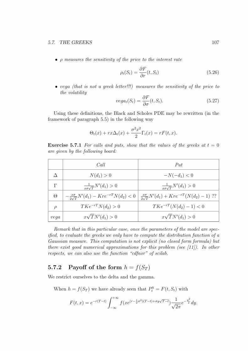
5.7. THE GREEKS 107

• ρ measures the sensitivity of the price to the interest rate

ρt(St) =∂F

∂r(t, St) (5.26)

• vega (that is not a greek letter!!!) measures the sensitivity of the price tothe volatility

vegat(St) =∂F

∂σ(t, St). (5.27)

Using these definitions, the Black and Scholes PDE may be rewritten (in theframework of paragraph 5.5) in the following way

Θt(x) + rx∆t(x) +σ2x2

2Γt(x) = rF (t, x).

Exercise 5.7.1 For calls and puts, show that the values of the greeks at t = 0are given by the following board:

Call Put

∆ N(d1) > 0 −N(−d1) < 0

Γ 1xσ√TN ′(d1) > 0 1

xσ√TN ′(d1) > 0

Θ − xσ2√TN ′(d1)−Kre−rTN(d2) < 0 xσ

2√TN ′(d1) +Kre−rT (N(d2)− 1) ??

ρ TKe−rTN(d2) > 0 TKe−rT (N(d2)− 1) < 0

vega x√TN ′(d1) > 0 x

√TN ′(d1) > 0

Remark that in this particular case, once the parameters of the model are spec-ified, to evaluate the greeks we only have to compute the distribution function of aGaussian measure. This computation is not explicit (no closed form formula) butthere exist good numerical approximations for this problem (see [11]). In otherrespects, we can also use the function “cdfnor” of scilab.

5.7.2 Payoff of the form h = f(ST )

We restrict ourselves to the delta and the gamma.

When h = f(ST ) we have already seen that P ht = F (t, St) with

F (t, x) = e−r(T−t)∫ +∞

−∞f(xe(r−

12σ2)(T−t)+σy

√T−t)

1√2πe−

y2

2 dy.


Proposition 5.7.1 We have

∆t(x) = e−r(T−t)E∗[

WT−t

xσ(T − t)f(SxT−t)

](5.28)

and

Γt(x) = e−r(T−t)E∗[(

−WT−t

x2σ(T − t)+W 2T−t − (T − t)

(σ(T − t)x)2

)f(SxT−t)

](5.29)

where (Sxt ) is (under P ∗) the geometric B.M with initial condition Sx0 = x.

Proof: We only prove (5.28), the method being the same for (5.29). We firstsuppose that f ∈ C1

K(R,R). (For the general case we use approximations...)

Using differentiation under the integral sign, we have

∆t(x) = e−r(T−t)∫ +∞

−∞

∂

∂xf(xe(r−

12σ2)(T−t)+σy

√T−t)︸︷︷︸

g(x,y)

1√2πe−

y2

2 dy.

But∂g

∂x(x, y) =

1

xσ√T − t

∂g

∂y(x, y).

Thus by using integration by parts,

∆t(x) =e−r(T−t)

xσ√T − t

∫ +∞

−∞f(xe(r−

12σ2)(T−t)+σy

√T−t)

y√2πe−

y2

2 dy.

Under P ∗, dSxt = rSxt dt+ σSxt dWt so

Sxt = xe(r−12σ2)t+σWt ,

thus,

∆t(x) = e−r(T−t)E∗[

WT−t


].2

Exercise 5.7.2 Show that

vegat(x) = x2TσΓt(x).

5.8. BLACK AND SCHOLES IN PRACTICE 109

5.7.3 Practical use of ∆ and Γ

In the framework of paragraph 5.5 we have seen that ∆t(St) has an importantfinancial interpretation: It is the quantity of risky asset to put in the hedgingportfolio at time t. Thus Γ represents the sensitivity of this quantity of riskyasset to variations of the underlying. Thus Γ is a measure of by how much or howoften a position must be rehedged in order to maintain a delta neutral position.Since in real life markets transaction costs can be large (contrary to our theo-retical hypothesis) Γ is very important for the cost-effectiveness of our hedgingstrategy. That’s why its knowledge is fundamental.

5.8 Black and Scholes in practice

(See also the Appendix)

5.8.1 Estimating volatility σ

Hedging and pricing strategies only depend on a unique and constant parameternot directly observable: the volatility (b disappears in the risk neutral universe)that is the most important and elusive quantity in the modern theory of deriva-tives. The problem of its estimation naturally arises.

One way to proceed is to use historical data. Let T ∈ R+. From observationsof the dynamic of the stock in the past [−T , 0], we can estimate σ by statisticalmethods. First we suppose that the dynamic in the intervall [−T , 0] is the sameas in the intervall [0, T ]. Let N ∈ N∗ be the number of observations, the randomvariables

Y N1 = Log

(S0

S−TN

), . . . , Y N

N = Log

(S−T

S−(N−1)TN

)are, under the historical probability, a N -sample of a

N ((b− σ2

2)T

N, σ2 T

N).

The most common estimator of σ is the empirical variance

σ =

√√√√ N

T (N − 1)

N∑i=1

(Y Ni − Y )2

where

Y =1

N

N∑i=1

Y Ni .


In practice, we take T = T to exclude the old and meaningless data. Remarkthat in real markets, the choice of N is limited by the frequence of the observedquotations. Moreover, more complicated procedures (GARCH models) may beused for a better understanding of this problem.

5.8.2 Pricing and Hedging

To determine the price of a financial product, the practitionner uses the formula

P h0 = E∗[e−r(T )f(ST )].

After that, he adopts the delta hedging strategy to eliminate (in theory) therisk due to randomness. This means that the number of assets held (∆t(St) at


time t for the risky one) must be continuously changed to maintain the position.

In reality, the portfolio is rehedged in discrete time because:

a) physical transactions are inevitably discrete

b) costs to buy or sell limit the number of transactions.

That’s why some risks associated with the model will appear. This is one ofthe most important problem of continuous time modelization.

In practice on a time intervall [t, t+h], the seller computes ∆ in t. The questionis to know if he may keep its position until t+h without commiting a big hedgingerror. In this way, he computes Γ in t. If the absolute value of Γ is big, the sellermust rebalanced the portfolio between t and t + h. If the Γ is small enough hemay maintains its position. Remark that there is an important duality betweena “good” hedging and its cost. That’s why the price of a contingent claim maybe seen in the following way:

Real price = Theoretic price (cost of the theoretic hedging) + transaction costs+ profit marging.

Remark that the vega also has an important role in the precautions to takefor the estimation of σ (preceding part).

5.8.3 Numerical computations of prices, of ∆ and of Γ

As far as Calls and Puts are concerned, prices, ∆ and Γ are given by explicitformulas (i.e closed form formulas). From a numerical point of view, we onlyhave to compute the distribution function of a N (0, 1) (its a classical problem,see for example the command “cdfnor” of scilab). Unfortunatly, when the payoffis more complicated such formulas are no more availlable and we have to usesome approximation tools e.g Monte Carlo methods (see [3]).

Reminder: The Monte Carlo method is based on the SLLN: Let (Xn) be asequence of i.i.d random variables such that X ∈ L1. Putting Sn = X1 + ...+Xn,we have

Snn

→a.s and L1

E[X1].

This result provides approximate solutions to perform expectations. (Remarkthat the speed of convergence is given by the C.L.T).

Here we have to evaluate


F (t, x) = e−r(T−t)E∗ [f(SxT−t)], ∆t(x) =

∂F

∂x(t, x) and Γt(x) =

∂2F

∂x2(t, x)

where (Sxt ) is a geometric Brownian motion with initial condition Sx0 = x.

For F (t, x), we may use the classical Monte Carlo method because a N -sampleof (SxT−t) is easy to simulate. For the other quantities (first and second derivativeswith respect to x ), one classical way is to use finite difference schemes i.e to usethe following approximations (think about Taylor formula...)

∆t(x) ≈F (t, x+ h)− F (t, x− h)

2h

Γt(x) ≈F (t, x+ h) + F (t, x− h)− 2F (t, x)

h2

where h is small enough and where F (t, x + h), F (t, x − h) and F (t, x) are per-formed by Monte Carlo method.

Problem for the greeks:

• This method embodies two different errors: discretization of the derivativefunction by a finite difference (choice of h???) and imperfect estimation ofthe option prices F (t, x+ h), F (t, x− h) and F (t, x)

• In the case of a strongly discontinuous payooff function, a well known factis its poor convergence to the exact solution.

To overcome this problem, we use proposition 5.7.1. In fact, we have provedthat

∆t(x) = e−r(T−t)E∗[

WT−t


]and

Γt(x) = e−r(T−t)E∗[(

−WT−t

x2σ(T − t)+W 2T−t − (T − t)

(σ(T − t)x)2

)f(SxT−t)

].

Thus, in the Black-Scholes model theses quantities may be performed withoutfinite differences.

Avantages:


• Only one error (MC)

• Weight independent of the payoff

• More efficient for Γ (second derivative) than for ∆ (first derivative).

Exercise 5.8.1 Consider a digital charracterized by its payoff IST≥K a T .

a) Show that F (0, x) = e−rTKN(d), ∆0(x) = e−rT

xσ√Tn(d) and Γ0(x) = e−rT

x2σ2Tn(d)

(d+ σ

√T)

where n is the density function of a N (0, 1) and where d =log( x

K)+(r−σ2

2)(T )

σ√T

.

b) Using scilab, compute ∆0(x) and Γ0(x) using the two preceding methods.Compare the results.

c) Answer to the preceding questions in the case of a corridor option ( PayoffIK2≥ST≥K1).

d) Define an empirical typology of option for which the weighted MC methodis more efficient than the traditional finite difference one.

Simulations

Using the preceding notations we takex = 100, K = 100, σ = 0, 15, r = 0, 05,T = 1, K1 = 95, K2 = 105.

Delta Call

0,64

0,645

0,65

0,655

0,66

0,665

0,67

1 5 9 13 17 21 25 29 33 37 41 45 49 53 57 61 65 69 73 77 81 85 89 93 97

Nbre de Simulations (10E4)

del

ta

Mall

DF

Valeur Theo:0,6584855


Gamma Call

0,0225

0,023

0,0235

0,024

0,0245

0,025

0,0255

1 5 9 13 17 21 25 29 33 37 41 45 49 53 57 61 65 69 73 77 81 85 89 93 97

Nbre simulations(10E4)

Gam

ma Mall

DF

Valeur theo 0,0244688

Delta Digitale

0,02

0,0203

0,0206

0,0209

0,0212

0,0215

0,0218

0,0221

1 5 9 13 17 21 25 29 33 37 41 45 49 53 57 61 65 69 73 77 81 85 89 93 97

Nbre simulations (10E4)

Del

ta

Mall

DF

Valeur Theo 0,0211279


Gamma Digitale

-0,0015

-0,0014

-0,0013

-0,0012

-0,0011

-0,001

-0,0009

-0,0008

-0,0007

-0,0006

-0,0005

1 5 9 13 17 21 25 29 33 37 41 45 49 53 57 61 65 69 73 77 81 85 89 93 97

Nbre Simulations (10E4)

Gam

ma Mall

DF

Valeur Theo 0,001058

Delta Corridor

-0,0052

-0,0047

-0,0042

-0,0037

-0,0032

1 5 9 13 17 21 25 29 33 37 41 45 49 53 57 61 65 69 73 77 81 85 89 93 97

Nbre de simulation (10E4)

Del

ta

Mall

DF

Valeur Théo: -0,0041146


Gamma Corridor

-0,002

-0,0015

-0,001

-0,0005

1 5 9 13 17 21 25 29 33 37 41 45 49 53 57 61 65 69 73 77 81 85 89 93 97

Nbre de simulations (10E4)

Gam

ma Mall

DF

Valeur Theo: -0,0009170

5.9 “Splendeurs et miseres“ of the Black Sc-

holes model

In spite of some unrealistic assumptions (some of them will be discuss hereafter),the Black-Scholes model remains a fundamental tool in modern finance. Theaim of this part is to introduce some important questions to continue the studybeyond this elementary lecture.

5.9.1 Advantages

Options have existed for centuries, but a major constraint upon their usefulnesswas the enormous difficulties of their pricing. In a world where very little wasknown about how options should be priced, trading options was a mixture ofguesswork and gambling, and very few economic agents participated in optionsmarkets. With the analytical capabilities created by Black and Scholes, the optionhas become a mainstream instrument ([13]), with millions of users all over theworld being able to meaningfully think about option pricing (within just a fewmonths after the Black–Scholes paper was published, Texas Instruments startedselling hand calculators which had the capability of evaluating the Black–Scholesformula!!!).

5.9. “SPLENDEURS ET MISERES“ OF THE BLACK SCHOLES MODEL117

From an academic point of view, Scholes (and Merton...) received the 1997Nobel Prize in Economics for this and related work; though ineligible becauseof his death in 1995, the Swedish academy broke with tradition and mentionedBlack as a contributor.

How to explain such a success???

Simplicity and theoretical efficiency

The Black-Scholes model only depends on a parameter not directly observable:the volatility that is a measure of the sensitivity to randomness (the stationarityof returns implying the possibility to use statistical methods to estimate thisparameter). Moreover, the prices and the hedging strategies are perfectly andeasily known in the case of the simplest (and fundamental) contingent claims (e.gcall and put). Finally, in this framework there is (in theory cf [18]) no risk dueto randomness.

Several view points

For more complicated financial products, we know that prices may only beobtained by numerical methods (no closed form formula). The Black Scholesmodel is interesting because two complementary approaches may be used in thiscase: A deterministic one linked to the approximation of solutions of P.D.E bydiscretization schemes and a probabilistic one based on Monte Carlo methods.We refer the reader to [7] and [19] for barrier options and to [12] and [20] forasian ones.

A self fulfilling prophecy???

Fisher Black: “Les operateurs savent maintenant utiliser la formule et lesvariantes. Ils l’utilisent tellement bien que les prix de marche sont generalementproches de ceux donnes par la formule, meme lorsqu’il devrait exister un ecartimportant...”

The Black–Scholes formula is considered by some economists to be a “selffulfilling prophecy” in the following sense: The formula relies on several unrealisticassumptions, the most important of which is the assumption that transactionscosts are zero. In reality, the trading involved in maintaining the riskless positionin continuous time would involve significant transactions costs. Yet, option pricesin the real world are remarkably close to those predicted by the Black–Scholesformula. One possibility is that if a sufficiently large mass of traders uses theBlack–Scholes formula as a working approximation, then the formula becomestrue. In this sense, it may be the case that the modern economy has beensteered in a certain direction because the Black–Scholes formula was discoveredin 1973.


5.9.2 Limites

The log-normal hypothesis

We refer the reader to [17] for more details on this topic.

The first modern attempt at analyzing options dates back to the year 1900,when the young French mathematician Louis Bachelier wrote a dissertation atSorbonne titled The Theory of Speculation. Bachelier was the first person tothink about financial prices using the modern tools of probability theory. Inparticular, he thought that it was possible to model the dynamic of an asset by a“good” probability distribution that had the properties of the Brownian motion.The approach that he took and many of the results that he obtained were farahead of their time. As a consequence, they were to lie dormant for sixty years.

Sixty five years later, Samuelson was the first to use the geometric Brown-ian motion (instead of the Brownian motion) to impose positivity conditions onprices.

From a technical point of view, these hypotheses (gaussian assumptions) werefruitful, in particular, they allowed the study of the equilibrium of financial mar-kets (see Markovitz, Sharpe and Linter) that’s why Black and Scholes used thisframework for their option pricing theory.

Nevertheless, in the middle of the sixties, Benoit Mandelbrot published anempirical research into the distribution of cotton prices based on a very longtime series which found that, contrary to the general assumption that these pricemovements were normally distributed, they instead followed a pareto-levy distri-bution. In particular, in a normally distributed market, crashes and booms arevanishingly rare, in a pareto-levy one crashes (extreme values) occur and are asignificant component of the final outcome.

This important problem is still an active field of research including the studyof ARCH, stochastic volatility or fractal models.

σ constant?

We refer the reader to [8] for more details on this topic.You may consult the Web site “www.ivolatility.com” to obtain numerical data

for the volatility of some american underlying.

In the Black Scholes model, the volatility is the only parameter not directlyobservable on the market. Since some elementary financial products are quotedon derivatives markets (e.g european calls) it is possible, using the market data,to have some knowledge on this parameter. In fact, remind that the price of a


call is given by the following formula

Ct = StN(d1(t, St))−Ke−r(T−t)N(d2(t, St))

where

d1(t, x) =log( x

K) + (r + σ2

2)(T − t)

σ√T − t

and d2(t, x) =log( x

K) + (r − σ2

2)(T − t)

σ√T − t

.

Thus, the price of the call is a strictly increasing function of the historical volatilitybecause

∂C

∂σ(t, x) = x

√T − tN ′(d1) > 0.

So, if we observe on the market the price at time t of a european call on therisky asset (of maturity T and strike K) (this observed price is denoted byCObst (x, T,K)), there exists a unique real number σimpl such that

CObst (x, T,K) = Ct(x, T,K, σ

impl).

Remark 5.9.1 The effective computation of the implicit volatility may be clas-sically done using Newton or bisection type methods .

In the framework of Black and Scholes, the implicit volatility should be equalto the historical one for all considered options. In practice, it is not the case. Wemay observed that

• The implicit volatility is greater than the historical one

• The implicit volatility both depends on the maturity and on the strike.

For the second point, the following graph shows the strike dependency of thevolatility of a european call (here the underlying is quoted on the american S&P500 market). The shape of the curve is really significant and called a smile ofvolatility. In fact, for 500 ≤ K ≤ 1400, we can see that the function is nonin-creasing (skew phenomenon) and when the strike is big it becomes nondecreasing(smile phenomenon).


400 600 800 1000 1200 1400 16000.0

0.1

0.2

0.3

0.4

0.5

0.6

0.7

0.8

vol implicite du call (sur une action du S&P 500) en fonction du strike

Figure 5.1: An example of volatility smile

Roughly speaking, several empirical considerations may partially highlight thisfundamental phenomenon:

• The implicit volatility is bigger for the options that are out of the money(K 6= S0). The market seems to give a greater probabilities to extremevalues than the ones observed in a log-normal model. (links with the pre-ceding paragraph).

• The smile may be explained by the fact that the market is less liquid forextreme strikes.

Remark 5.9.2 Today, practitioners make their reasonings in terms of implicitvolatility instead of price. Black Scholes formula has became a privileged transla-tor.

To conclude, remark that in spite of the preceding considerations, praction-ers use extensively Black-Scholes option pricing formula even to evaluate optionswhose underlying is known to not satisfy the Black-Scholes hypothesis of a con-stant volatility. In fact, when the Γ of an option is nonnegative (i.e convex payoff)it can be shown that if the trader chooses a constant volatility bigger than the


real one (that may be stochastic....) the value of his hedging portfolio will alwaysbe greater then the payoff of the option at maturity (he never looses money).This fundamental property is known as the robustness of the Black and Scholesformula. In some sense it moderates the preceding criticisms.

Let us see this phenomenon in the case of a european call of maturity T andstrike K.

Suppose that the price of the stock is given (under the risk neutral probabilityby) by

dSt = rStdt+ ΣtStdBt

where Σt is a regular stochastic process.In spite of this dynamic, the practitioner computes his hedging portfolio using

the Black and Scholes formula with a constant volatility σ. Thus the quantity ofrisky asset is given by ∆BS(t, St) with ∆BS(t, x) = ∂CBS

∂x(t, x) where CBS is the

Black-Scholes price (proposition 5.6.1). The value at time t of this portfolio isequal to

Vt = ∆BS(t, St)St +H0t S

0t

and the self-financing condition

dVt = ∆BS(t, St)dSt +H0t dS

0t

implies that

dVt = rVtdt+ ∆BS(t, St)(dSt − rStdt)

with initial condition

V0 = CBS(0, S0).

Thus, at time T the hedging error is

eT = VT − CBS(T, ST )︸︷︷︸(ST−K)+

.

By Ito formula,

dCBS(t, St) =

(∂CBS∂t

(t, St) +1

2

∂2CBS∂x2

(t, St)Σ2tS

2t

)dt+

∂CBS∂x

(t, St)dSt.

But Black-Scholes PDE (5.15) ensures that

∂CBS∂t

(t, x) + rx∂CBS∂x

(t, x) +σ2x2

2

∂2CBS∂x2

(t, x) = rCBS(t, x).

Then, we obtain the following E.D.O


d(Vt − CBS(t, St)) = r(Vt − CBS(t, St))dt−1

2

∂2CBS∂x2

(t, St)(Σ2t − σ2)S2

t dt.

Finally

eT =erT

2

∫ T

0

e−rt∂2CBS∂x2

(t, St)(−Σ2t + σ2)S2

t dt.

So, When σ ≥ Σt a.s then eT ≥ 0 a.s, the Black-Scholes price dominates the realprice.

Bibliography

[1] L. Bachelier: Theorie de la speculation, Annales scientifiques de l’ecolenormale superieure, 17, 21-86, 1900.

[2] F. Black, M. Scholes: The pricing of options and corporate liabilities,Journal of Political Economy, 81, n3, 637-654, 1973.

[3] N. Bouleau, D. Talay : Probabilites numeriques, INRIA, 1992.

[4] J.C. Cox, S.A. Ross, M. Rubinstein: Options pricing: a simplifiedapproach, Journal of Financial Economics, 7, 229-263, 1979.

[5] J.-P. Fouque, G. Papanicolaou and K. R. Sircar: Derivatives inFinancial Markets with Stochastic volatility, Cambridge University Press,2000.

[6] E. Fournier and al: Applications of Malliavin calculus to Monte-Carlomethods in finance, Finance and Stochastics, 3, 391-412, 1999.

[7] H. Gemam, M. Yor: Pricing and Hedging Double-Barrier Options : AProbabilistic Approach, Mathematical Finance, vol. 6, Issue 4, 1996.

[8] M.H. Grouard, S. Levy, C. Lubochinsky: La volatilite boursiere : desconstats empiriques aux difficultes d’interpretation, Banque de France, RSF,2003.

[9] J.C. Hull: Options, Futures and other derivatives, Prentice Hall, 2003.

[10] N. El Karoui, M. Jeanblanc-Picque, S. Shreve: Robustness of theBlack and Scholes Formula, Mathematical Finance, vol. 8, Issue 2, 93-126,1998.


[12] B. Lapeyre, E Temam: Competitive Monte Carlo Method for the pricingof asian options, Journal of computational finance, 2002.

123

124 BIBLIOGRAPHY

[13] D. MacKenzie,: An Equation and its Worlds: Bricolage, Exemplars, Dis-unity and Performativity in Financial Economics, Social Studies of Science33 (6): 831-868, 2003.

[14] R. Merton: Theory of Rational Option Pricing, Bell Journal of Economicsand Management Science, 4, 141-183, 1973.

[15] D. Nualart: The Malliavin Calculus and related Topics, Springer Verlag,New York, 1995.

[16] B. Oksendal: An Introduction to Malliavin Calculus with Applications toEconomics, 1996.

[17] B. Pochart: Processus multifractals en finance et valorisation d’optionspar minimisation de risques extremes, These de Doctorat, 2003.

[18] F.E. Racicot, R. Theoret: Simulations de la couverture delta et de lacouverture delta-gamma d’un portefeuille dans le cadre du modele de Black etScholes, RePAd Working Paper Series UQO-DSA-wp122006, Departementdes sciences administratives, UQO.

[19] R. Zvan, K. R. Vetzal, and P. A. Forsyth.: PDE Methods for PricingBarrier Options, Journal of Economic Dynamics and Control, 1998.

[20] R. Zvan, K. R. Vetzal, and P. A. Forsyth.: Robust numerical meth-ods for PDE models of asian options , J. Computational Finance, 1, 39-78,1998.

BIBLIOGRAPHY 125

APPENDIX (IN FRENCH FORTHE MOMENT.......)

126 BIBLIOGRAPHY

Simulation d’un mouvementBrownien

Simuler?Simuler le mouvement Brownien (ou plus generalement un processus stochas-

tique) revient a calculer de maniere numerique et approchee une trajectoire (ouune famille de trajectoires) de ce processus (ie t ∈ [0, 1] → Bt(w) pour w fixe).

D’apres ce qui a ete dit dans le cours, plusieurs methodes s’offrent a nous. J’endetaillerai deux.

Representation de Wiener (1923)Soit (gn) une famille de N (0, 1) independantes definies sur un espace (Ω,A, P ).On utilise la formule suivante

Bt(w) =

√8

π

∞∑n=1

sin(nt)

ngn(w) (30)

ou la serie converge uniformement presque surement sur [0, 1].

L’algorithme de simulation se decompose de la maniere suivante:

1) La formule etant une somme infinie on doit choisir un indice k0 suffisammentgrand (par ex k0 = 10000) pour valider l’approximation suivante

Bt(w) '√

8

π

k0∑n=1

sin(nt)

ngn(w). (31)

2) Je simule les variables aleatoires gaussiennes en utilisant la methode de BoxMuller (Je suppose ici que k0 est pair pour la commodite de la redaction):

a) Je fais k0 appels a la fonction random de mon ordinateur. J’obtiens k0

elements de l’intervalle [0, 1] que je note U1(w),....,Uk0(w) et qui correspondent aune realisation de k0 variables aleatoires independantes distribuees suivant uneU([0, 1]).

b) ∀j ∈ 1, k02, je calcule (en faisant appel aux commandes π, cos, sin, log et

√de scilab)

g2j−1(w) =√−2log(U2j−1(w))cos(2πU2j(w))

et

BIBLIOGRAPHY 127

g2j(w) =√−2log(U2j−1(w))sin(2πU2j(w)).

Ainsi, d’apres l’exercice vu en cours les g1(w),....,gk0(w) correspondent a unerealisation de k0 variables aleatoires independantes distribuees suivant uneN (0, 1).

3) Je definis en faisant une boucle la fonction

t→√

8

π

k0∑n=1

sin(nt)

ngn(w).

4) je trace cette fonction.

On obtient le resultat suivant sous scilab avec k0 = 1000

0.0 0.1 0.2 0.3 0.4 0.5 0.6 0.7 0.8 0.9 1.0!1.2

!1.0

!0.8

!0.6

!0.4

!0.2

0.0

0.2

Methode de donsker

je rappelle le resultat du cours sur lequel est fondee la methode.

On se donne une famille (Uk)k∈N∗ de variables aleatoires independantes, centreeset reduites. Pour tout n ∈ N∗, on note Sn = U1 + ... + Un la n-ieme sommepartielle. Considerons alors l’interpolation polygonale de rang n de la serie des

128 BIBLIOGRAPHY

sommes partielles renormalisees: ∀t ∈ [0, 1], on pose

Xn(t) =1√n

[nt]∑k=1

Uk + (nt− [nt])U[nt]+1

. (32)

Theorem .0.1 La suite de processus continus (Xn) converge en loi dans C =C([0, 1],R) vers la loi du M.B i.e ∀f ∈ Cb(C,R), E[f(Xn)] → E[f(B)].

L’algorithme de simulation est alors le suivant:

1) La formule etant une serie infinie on doit choisir un indice k0 suffisammentgrand (par ex k0 = 10000) pour valider l’approximation suivante:

B(t)(w) ≈ 1√k0

[k0t]∑k=1

Uk(w) + (k0t− [k0t])U[k0t]+1(w)

. (33)

2) Je fais le choix de mes variables aleatoires U1,....,Uk0 centrees reduitesindependantes et je simule une realisation de ces variables (vous pouvez utilisersi vous le voulez les gaussiennes g1(w),....,gk0(w) et poser Uj(w) = gj(w) , per-sonnellement, j’ai fait un choix different....).

3) Pour tout j ∈ 1, k0 je calcule (en faisant une boucle)

Sj√k0

=U1 + ...+ Uj√

k0

.

4) Reste donc a tracer

t→ 1√k0

[k0t]∑k=1

Uk(w) + (k0t− [k0t])U[k0t]+1(w)

.

Contrairement a la forme qui peut paraıtre un peu barbare, ceci est en fait tressimple. En effet, la fonction n’est autre que la fonction lineaire par morceauxpassant par tous les points de la forme ( j

k0,Sj√k0

). Il existe sur tous les logiciels

de calcul matriciel (scilab, matlab) une fonction (appelee “plot’) permettant derealiser ceci sans travailler (et donc on en profite)!!!!

La simulation suivante a ete realisee sous scilab en choisissant les Ui de sorteque P (Ui = 1) = P (Ui = −1) = 1

2(pour la simulation des Ui je renvois aux

annexes du Lamberton-Lapeyre) et en prenant k0 = 10000.

BIBLIOGRAPHY 129

0.0 0.1 0.2 0.3 0.4 0.5 0.6 0.7 0.8 0.9 1.0 1.1!140

!120

!100

!80

!60

!40

!20

0

20

Exercice 1: Essayez de le faire vous meme en utilisant par exemple scilab quiest tres bien et gratuit!!! On peut le telecharger a l’adresse suivante:

“http://www.scilab.org/download/index download.php?page=release.html”.

Exercice 2: Faire un travail similaire pour la methode du point milieu.

130 BIBLIOGRAPHY

Quelques exercicesExercice 1: 1) Montrer que la variable aleatoire Xt =

∫ t0cos(s)dBs est bien

definie.

2) Montrer que (Xt)t∈[0,1] est un processus gaussien dont vous calculerez lamoyenne et la fonction de covariance.

3) Montrer que Xt = cos(t)Bt +∫ t

0sin(s)Bsds.

Exercice 2: Soit t ∈ [0, 1] et f ∈ L2([0, 1]), montrer que

E[Bt

∫ 1

0

f(s)dBs] =

∫ t

0

f(s)ds.

Exercice 2’: On cosnidere la suite (Zn)n∈N∗ de variables aleatoires definiespar

Zn =

∫ 1

0

(1 +s

n)ndBs

et on pose

Z =

∫ 1

0

esdBs.

1) Montrer que (Zn)n∈N∗ converge vers Z dans L2.2) Montrer que ∀s ∈ [0, 1],

0 ≤ s− nlog(1 +s

n) ≤ s2

2n.

En deduire que

0 ≤ es − (1 +s

n)n ≤ e1

2n.

3) En deduire que pour tout α > 0,∑n≥1

P (|Zn − Z| > α) <∞.

4) Montrer que la suite (Zn)n∈N∗ converge presque surement vers Z.

Exercice 3: Soit Xt la solution de l’EDS suivante:

dXt = (µXt + µ′)dt+ (σXt + σ′)dBt, X0 = 0.

On pose St = e(µ−σ2

2)t+σBt .

BIBLIOGRAPHY 131

1) Demontrer que d(XtS−1t ) = S−1

t [(µ′ − σσ′)dt+ σ′dBt].

2) En deduire une expression pour Xt.

Exercice 4: Dans le modele de Black et Scholes, calculer la probabilite qu’uncall europeen soit exerce.

Exercice 5: Soit St la solution de dSt = rStdt+ σStdBt.

1) Soit K ∈ R+, montrer que le processus

Mt = E

[(1

T

∫ T

0

Sudu−K

)+

|FBt

]est une martingale.

2) Montrer que si l’on pose ξt = S−1t

(K − 1

T

∫ t0Sudu

), on a

Mt = StE

[(1

T

∫ T

t

SuStdu− ξt

)+

|FBt

].

3) Soit φ(t, x) = E

[(1T

∫ Tt

Su

Stdu− x

)+

]. Montrer que Mt = Stφ(t, ξt).

4) Ecrire la formule d’Ito pour Mt et en deduire une EDP verifiee par la fonc-tion φ.

Exercice 6: Soit B un MB sous une probabilite P . Soit (Mt)t∈[0,1] une FBt

martingale (sous P ) telle que dMt = MtσdBt avec σ ∈ R et M0 = 1.

1) Verifier que M est a valeurs strictement positives.

2) Calculer dYt ou Yt = M−1t .

3) Soit Q la probabilite definie par dQdP

= MT . Determiner la loi de Y sous Q.

4) Montrer que

EP [(MT −K)+] = KEP [(K−1 −MT )+].

Exercice 7: Si Xt est solution d’une EDS de type

dXt

Xt

= r(t)dt+ σXt (dBt + λtdt)

132 BIBLIOGRAPHY

le parametre (eventuellement aleatoire) σX est appele la volatilite locale de X.Dans le cadre du modele de Black et Scholes, montrer que la volatilite local d’uncall est plus grande que la volatilite historique (ce phenomene est connu sous lenom d’effet levier).

Exercice 8: Trouver (θt)t∈[0,T ] ∈ L2prog(Ω×[0, T ]) tel que F = E[F ]+

∫ T0θsdBs

pour

1) F = BT ,

2) F =∫ T

0Bsds,

3) F = B2T ,

4) F = eBT .

Exercice 9: On se place dans le cadre du modele de Black et Scholes vu encours. On note C(St, t, T,K) (resp. P (St, t, T,K)) le prix a l’instant t du call(resp. du put) de strike K et d’echeance T .

1) Expliciter P (St, t, T,K) en fonction de C(St, t, T,K).

2) On fixe dorenavant T0 ∈]0, T [. On considere l’option DF (depard forward)suivante: le detenteur de cette option recoit a l’instant T0 un call d’echeance Tet de strike ST0 .

a) Quel est le payoff terminal en T d’une telle option?

b) Prouver que le prix en T0 de cette option peut s’ecrire ST0C(1, T0, T, 1).

c) Montrer que le prix a 0 ≤ t ≤ T0 est C(St, T0, T, St).

3) On considere maintenant l’option CH (chooser) suivante: le detenteur decette option choisit a la date T0 si l’option en question est un call ou un putd’exercice K et d’echeance T fixes a l’avance.

a) Quel est le prix a T0? Montrer qu’il peut se mettre sous la forme

C(ST0 , T0, T,K) + (Ke−r(T−T0) − ST0)+.

c) Trouver le prix a 0 ≤ t ≤ T0 de cette option. Donner un portefeuille fi-nancier statique de couverture entre 0 et T0.

Exercice 9: Exercice 1.3.4 du poly.

BIBLIOGRAPHY 133

Exercice 10: Soit Yt = h(t)dt+dBt et rt = σ(t)Yt ou h et σ sont des fonctions

de classe C1. On souhaite calculer E[e−

R t0 rsds

].

1) Exprimer dr.

2) Soit LHt = eR t0 H(s)dBs− 1

2

R t0 H

2(s)ds. Justifier que E[LHT ] = 1 pour toute fonctionH continue. En deduire que

E[eh(T )BT−

R T0 h′(s)Bsds− 1

2

R T0 h2(s)ds

]= 1.

3) En utilisant Lht , montrer que

E[e−

R t0 rsds

]= E

[eh(T )BT−

R T0 (h′(s)+σ(s))Bsds− 1

2

R T0 h2(s)ds

].

4) Calculer cette quantite.

Exercice 11: On considere un actif dont la dynamique est donnee par

dSt = St((r − δ)dt+ σdBt), S0 = x

.

1) Montrer que dans le cadre du modele de Black et Scholes cette dynamiquemodelise (sous la probabilite risque neutre Q) le prix d’un actif risque versant desdividendes au taux continu r.

2) On souhaite evaluer un actif contingent sur S. Il s’agit donc d’evaluer

EQ[h(ST )e−r(T−t)].

Quelle est la valeur de cet actif dans le cas ou h(x) = (xα −K)+.

3) On suppose r = δ. On pose dQ = ST

xdQ et Zt = x2

St.

a) Justifier rapidement que l’on definit ainsi un changement de probabilite.b) Quelle est la dynamique de Zt sous Q?c) Montrer que pour toute fonction borelienne bornee,

1

xEQ[STf(

x2

ST)] = EQ[f(ST )].

4) On repasse au cas general. Montrer que le processus Sa est une martingalepour une valeur de a que l’on precisera. Montrer alors que pour toute fonctionborelienne bornee,

134 BIBLIOGRAPHY

1

xaEQ[SaTf(

x2

ST)] = EQ[f(ST )].

5) On se place dans le cas h(x) = xβ(x − K)+. Montrer que h(ST ) s’ecritcomme difference de deux payoffs correspondants a des call europeens de sousjacents Sβ+1 et Sβ avec des strikes que l’on determinera. Conclure.

Exercice 12: Probleme 1 (page 85) du Lamberton-Lapeyre.

Exercice 13: Probleme 4, partie 2 (page 91) du Lamberton-Lapeyre.

Exercice 14: Probleme 2, (page 86) du Lamberton-Lapeyre.

BIBLIOGRAPHY 135

Test 10/06 (1H)

Exercice 1: Soit (Ω,A, P ) un espace de probabilite equipe d’une filtration(Ft)t∈R+ et (Xt)t∈R+ un processus reel defini sur (Ω,A, P ).

a) Quand dit on que le processus (Xt)t∈R+ est adapte?

b) Quand dit on que le processus (Xt)t∈R+ est progressivement mesurable?

c) Y a t-il un lien entre les deux notions?

d) On suppose que (Xt)t∈R+ est adapte et continu a droite. On veut montrerque (Xt)t∈R+ est progressivement mesurable. Pour T ∈ R+, on definit la suite(Xn)n∈N∗ de processus par Xn

t = XMin(T,([ntT

]+1)Tn

), ∀t ∈ [0, T ].

d1) Montrer que ∀t ∈ [0, T ], Xnt →p.pXt.

d2) Montrer que ∀n ∈ N∗, ∀Γ ∈ B(R) on a

(t, ω); 0 ≤ t ≤ T,Xnt ∈ Γ ∈ B([0, T ])×FT .

d3) Conclure.

L’exercice suivant est un exercice sur les martingales pas sur le M.B

Exercice 2: Soit (Bt)t∈[0,1] un processus stochastique sur un espace de prob-abilite (Ω,A, P ). On note (FB

s = σ(Bu, u ≤ s))s∈[0,1] sa filtration naturelle. Onsuppose que les hypotheses suivantes sont verifiees:

a) B0 = 0 P -p.s.

b) (Bt)t∈[0,1] est continu.

b) Si t > s, Bt −Bs est independant de FBs .

c) Si t ≥ s, Bt −Bs suit une N (0, t− s).

En utilisant les proprietes de l’esperance conditionnelle montrer que les pro-cessus (Bt)t∈[0,1], ((Bt)

2 − t)t∈[0,1] et (eθBt−θ2 t2 )t∈[0,1] (θ ∈ R) sont des (FB

t )t∈[0,1]

martingales continues de carre integrable.

Exercice 3 Montrer que la limite de toute suite de variables aleatoires gaussi-ennes qui converge dans L2 est gaussienne.

136 BIBLIOGRAPHY

Master IRFA

Examen de Calcul Stochastique 12/06

3 Heures

Les notes de cours et les calculatrices ne sont pas autorisees. La clarte et laconcision des reponses seront des elements determinant de la notation.

Indication de Bareme: I) 6 points, II) 8 points, III) 6 points. Laquestion III) 3 est hors bareme et vaut 3 points.

Exercice I: On se place dans le cadre du modele de Black et Scholes: ladynamique de l’actif risque entre 0 et T > 0 est donnee par l’EDS suivante

dSt = µStdt + σStdBt (34)

de condition initiale S0 = x0 > 0 ou µ ∈ R et σ ∈ R∗+.

a) On pose ∀n ∈ N, ∀j ∈ 0, ..., 2n, tnj = Tj2n . Montrer que

limn→+∞

1

T

2n−1∑j=0

(log

(Stnj+1

Stnj

))2

= σ2.

Expliquer l’interet de cette relation d’un point de vue statistique.

b) On considere un actif contingent h de la forme f(ST ). Rappeler la definitiondes grecques ∆ et Γ. Quel est leur interet pour le praticien?

c) Expliquer en 10 lignes maximum deux points faibles du modele de Black etScholes.

Exercice II: Modele de Black et Scholes avec parametres dependantdu temps

Nous reprenons le modele de Black et Scholes, en supposant que le prix del’actif sans risque est donne par

dS0t = r(t)S0

tdt; S00 = 1 (35)

et celui de l’actif risque par

dSt = µ(t)Stdt + σ(t)StdBt; S0 = x0 > 0 (36)

BIBLIOGRAPHY 137

ou r, µ et σ sont dans C([0, T ],R) et ou B est un mouvement Brownien standardsous la probabilite historique P . On supposera de plus que inf

t∈[0,T ]σ(t) > 0.

1) En considerant le processus

Zt = Ste−

R t0 µ(s)ds−

R t0 σ(s)dBs+

12

R t0 σ

2(s)ds,

montrer que l’unique solution de (3) est donnee par

St = S0eR t0 µ(s)ds+

R t0 σ(s)dBs− 1

2

R t0 σ

2(s)ds.

2) Montrer qu’il existe une probabilite Q equivalente a P sous laquelle le prixactualise de l’actif risque est une martingale. Donner la densite de Q par rapporta P .

3) Soit (Ht = (θ0t , θt)t∈[0,T ]) une strategie financiere autofinancee dont la valeur

a t est notee Vt. Montrer que lorsque ( Vt

S0t)t∈[0,T ] est une martingale sous Q verifiant

VT = (ST −K)+ alorsVt = F (t, St)

ou

F (t, x) = EQ

[(xe

R Tt σ(s)dWs− 1

2

R Tt σ2(s)ds −Ke−

R Tt r(s)ds

)+

]et ou W est un mouvement Brownien standard sous Q.

4) Expliciter la fonction F et faire le lien avec la formule de Black et Scholes.Que peut on en deduire pour le prix d’un put d’echeance T et de strike K?

5) Construire une strategie de couverture pour le Call d’echeance T et de strikeK. Cette strategie est elle autofinancee?

6) Demontrer que F verifie une equation aux derivees partielles que vous ex-pliciterez.

Exercice III: Prix d’un zero coupon dans le modele de Hull et White

On considere le processus (r(t))t∈[0,T ] verifiant l’EDS suivante

dr(t) = [α(t)− β(t)r(t)]dt+ σ(t)dBt (37)

ou α, β et σ ∈ C([0, T ],R). On pose K(t) =∫ t

0β(s)ds

1) Calculer d(eK(t)r(t)). En deduire que

138 BIBLIOGRAPHY

r(t) = e−K(t)

[r(0) +

∫ t

0

eK(u)α(u)du+

∫ t

0

eK(u)σ(u)dBu

].

2) Montrer que (r(t))t∈[0,T ] est un processus gaussien continu dont vous cal-culerez la moyenne et la fonction de covariance.

3) On pose Xt =∫ t

0eK(u)σ(u)dBu et YT =

∫ T0e−K(u)Xudu. Montrer que

YT → N

(0,

∫ T

0

e2K(u)σ2(u)

(∫ T

u

e−2K(y)dy

)2

du

).

4) En deduire la loi de∫ T

0r(s)ds.

5) Donner le prix du zero coupon

E[e−

R T0 r(s)ds

].

BIBLIOGRAPHY 139

Master IRFA

Calcul Stochastique 06/07

2 Heures


Indication de Bareme: I) 7 points, II) 8 points, III) 5 points, .

Exercice I: Autour du cours

1) Exposer de maniere precise et concise une methode de simulation du mou-vement brownien.

2) On pose Xt =∫ t

0cos(s)dBs.

2.a) Montrer que (Xt)t∈[0,1] est un processus gaussien dont vous calculerez lamoyenne et la fonction de covariance.

2.b) Montrer que Xt = cos(t)Bt +∫ t

0sin(s)Bsds.

3) Demontrer que le mouvement brownien est un processus a variations infiniessur tout intervalle.

4) En utilisant le theoreme approprie vu en cours, demontrer l’existence d’uneprobabilite risque neutre dans le modele de Black-Scholes

Exercice II: Moments de la solution de l’EDS de Black-Scholes

On considere l’EDS de Black-Scholes

dSt = µStdt + σStdBt (38)

de condition initiale S0 = x0 > 0 ou µ ∈ R et σ ∈ R∗+.

a) Montrer qu’une solution de l’EDS est donnee par

St = x0e(µ−σ2

2)t+σBt .

Montrer que la solution ci-dessus est unique.

140 BIBLIOGRAPHY

b) Calculer E[St].

c) Pour α ≥ 2, determiner l’EDS verifiee par Sαt .

d) Montrer soigneusement que

E[Sαt ] = xα0 +

∫ t

0

βE[Sαs ]ds

ou β = αµ+ α(α−1)σ2

2.

e) En deduire queE[Sαt ] = xα0 e

βt.

Exercice III: Changement de numeraire

On considere deux actifs financiers dont le prix est donne par les processusd’Ito suivants

dS1t = µ1

tdt+ σ1t dBt

dS2t = µ2

tdt+ σ2t dBt

ou les integrands sont dans L2prog(Ω× [0, T ]).

Soient Φ1 et Φ2 deux processus stochastiques progressivement mesurables etbornes.

On definit ∀t ∈ [0, T ],Xt = Φ1

tS1t + Φ2

tS2t (39)

et on suppose que

dXt = Φ1tdS

1t + Φ2

tdS2t . (40)

a) Interpreter financierement (2) et (3).

b) Soit (Ut)t∈[0,T ] un processus d’Ito de la forme

dUt = U1t dt+ U2

t dBt.

Montrer qued(UX)t = Φ1

td(US1)t + Φ2

td(US2)t.

c) Donner une interpretation financiere simple de la question precedente.

BIBLIOGRAPHY 141

Master IRFA

Exam of Stochastic calculus 01/08

3 Heures

Notation: 1) 3 points, 2) 11 points, 3) 8 points.

Exercise 1: Course

1) Show that a stochastic process (Bt)t∈[0,1] is a standard brownian motionif and only if it is a continuous and centered gaussian process with covariancefunction Γ[s, t] = inf(s, t).

2) When (Bt)t∈R+ is a brownian motion, show that Bn

n→n→∞

0.

Exercise 2: Black-Scholes model, binary options, options on mean

We are in the framework of the Black-Scholes model: the dynamic of the nonrisky asset is given by

dS0t = rS0

tdt; S00 = 1 (41)

and the dynamic of the risky one by

dSt = µStdt + σStdBt; S0 = x0 > 0 (42)

where r, µ and σ are non negative real numbers and where B is a standard brow-nian motion under the historical probability P .

A] 1) Considering

Zt = Ste−µt−σBt+

12σ2t,

show that the unique solution of (2) is given by

St = S0eµt+σBt− 1

2σ2t.

2) Remind the Black Scholes formula for the price of a european call at time0 ≤ t ≤ T .

B] A binary option has a payoff IST≥K at time T .

a) Compute the price of this option at time 0 ≤ t ≤ T .

b) Show that the associated delta and gamma are given ∀0 ≤ t ≤ T by

142 BIBLIOGRAPHY

∆t(x) =e−r(T−t)

xσ√T − t

n(d(t, x)) et Γt(x) =e−r(T−t)

x2σ2(T − t)n(d(t, x))

(d(t, x) + σ

√T − t

)where n is the density function of aN (0, 1) and where d(t, x) =

log( xK

)+(r−σ2

2)(T−t)

σ√T−t .

c) What is the interest of these quantities in finance?

d) Deduce (without computations) from a) the price of an option with a payoffequal to IST<K .

C] A european call on the mean is characterized by its payoff

(e1T

R T0 ln(St)dt −K)+.

1) show that the price at time t = 0 is given by

Z0N(d1)−Ke−rTN(d2)

where

Σ =σ√3, Z0 = S0e

−bT2−σ2T

12 ,

d1 =ln(Z0

K) + (r + Σ2

2)T

Σ√T

and d2 =ln(Z0

K) + (r − Σ2

2)T

Σ√T

and where N is the distribution function of a N (0, 1).

2) What is the composition of the associated hedging portfolio?

Exercise 3: Let B be a standard brownian motion under a probability P . Let(Mt)t∈[0,1] be a FB

t martingale (under P ) such that dMt = MtσdBt with σ ∈ Rand M0 = 1.

1) Prove that M is a strictly positive process.

2) Compute dYt where Yt = M−1t .

3) Let Q be a probability defined by dQdP

= MT . Find the distribution of Yunder Q.

BIBLIOGRAPHY 143

4) Show that

EP [(MT −K)+] = KEP [(K−1 −MT )+].

5) Give a financial interpretation of this result.

144 BIBLIOGRAPHY

Master IRFA

Exam of Stochastic calculus 12/08

3 Heures


Indication de Bareme: I) 4, II) 8, III) 8.

Dans tout l’enonce (Bt)[0,T ] est un mouvement brownien standard defini sur unespace (Ω,A, P ). On notera, de plus, E l’esperance sous P et (Ft)[0,T ] la filtrationBrownienne.

Exercice I: Autour du cours

1) Montrer que le processus (B2t − t)[0,T ] est une martingale continue par rap-

port a la filtration Brownienne.

2) Dans le cadre du modele de Black-Scholes donnez (en utilisant la formulepour le call) le prix d’une option de vente a l’instant t. Quel est le portefeuillede couverture associe?

Exercice II: Ornstein-Uhlenbeck, Vasicek, CIR

On considere l’EDSdXt = αXtdt+ bdBt (43)

ou (α, b) ∈ R2 et X0 = x ∈ R.

1) En utilisant le processus Yt = e−αtXt montrez que l’unique solution de (1)est donnee par

Xt = eαt(x+ b

∫ t

0

e−αsdBs

).

2) Montrer que (Xt) est un processus gaussien dont vous calculerez les fonc-tions de moyenne et de covariance.

3) Montrer que (∫ t

0Xsds) est un processus gaussien dont vous calculerez les

fonctions de moyenne et de covariance.

4) Calculez E[eR T0 Xsds].

BIBLIOGRAPHY 145

5) En utilisant 1) montrez que l’equation

dZt = −α(a− Zt)dt+ bdBt (44)

ou a ∈ R et Z0 = z ∈ R admet une unique solution dont vous donnerez le formeexplicite.

6) On definit ∀t ∈ [0, T ], rt = X2t . Montrez que

drt = 2√rtbdBt + (2αrt + b2)dt.

Exercice III: Options asiatiques dans Black-Scholes

Nous reprenons ici le modele de Black et Scholes, en supposant que le prix del’actif sans risque est donne par

dS0t = rS0

tdt; S00 = 1 (45)

et celui de l’actif risque par

dSt = µStdt + σStdBt; S0 = x0 > 0 (46)

ou r, µ et σ sont des reels strictement positifs.

A] Montrez l’existence d’une probabilite Q equivalente a P telle que le proces-sus ( St

ert )t∈[0,T ] soit une martingale.

Quelle est la dynamique de (St) sous Q?B] On suppose maintenant r = 0 et que dSt = σStdWt ou (Wt) est un mouve-

ment Brownien standard sous Q

1) Soit K ∈ R+, montrer que le processus

Mt = EQ

[(1

T

∫ T

0

Sudu−K

)+

|FBt

]est une martingale.

Que represente cette quantite d’un point de vue financier?

2) Montrer que si l’on pose ξt = S−1t

(K − 1

T

∫ t0Sudu

), on a

Mt = StEQ

[(1

T

∫ T

t

SuStdu− ξt

)+

|FBt

].

146 BIBLIOGRAPHY

3) Montrer pour tout t ∈ [0, T ] que∫ Tt

Su

Stdu est independante de FB

t et que

ξt est FBt mesurable.

4) Soit φ(t, x) = EQ

[(1T

∫ Tt

Su

Stdu− x

)+

]. Montrer que Mt = Stφ(t, ξt).

5) Montrer que

dS−1t = S−1

t [(σ2)dt− σdBt]

et que

dξt = ξt[(σ2)dt− σdBt]−

dt

T.

6) Ecrire la formule d’Ito pour Mt et en deduire une EDP verifiee par la fonc-tion φ.

stochastic calculus: applications in finance - christophe chorro

Documents