Stabilized methods for compressible flows

Thomas J. R. Hughes

Institute for Computational Sciences and Engineering,

The University of Texas at Austin,

1 University Station C0200, Austin, TX 78712-0027, USA

Guglielmo Scovazzi∗

1431 Computational Shock- and Multi-physics Department,

Sandia National Laboratories,

P.O. Box 5800, MS 1319, Albuquerque, NM 87185-1319, USA

Tayfun E. Tezduyar

Mechanical Engineering, Rice University – MS 321,

6100 Main Street, Houston, TX 77005, USA

March 24, 2008

Abstract

This article reviews 25 years of research on stabilized methods for

compressible flow computations. An historical perspective is adopted

to document the main advances from the initial developments to

modern approaches.

Keywords: Stabilized methods, SUPG method, compressible flows.

1 Introduction

The development of stabilized methods began in the late 1970s. A numberof papers appeared in conference proceedings and in books emanating fromconferences. The first journal paper was that of Brooks and Hughes [5],which summarized early work on the subject. The application areas wereadvection–diffusion equations and the incompressible Navier–Stokes equa-tions. The first stabilized method was SUPG, an acronym for streamline

∗Sandia is a multiprogram laboratory operated by Sandia Corporation, a Lockheed

Martin Company, for the United States Department of Energy under contract DEAC04-

94-AL85000.

1

upwind/Petrov-Galerkin. At about the same time, the opportunity aroseto extend the method to the compressible Euler equations. Airframe man-ufacturers and aerospace agencies, such as NASA, were making significantinvestments in computational fluid dynamics and this provided funding.This was occurring at the time shortly after one of us, T. Hughes, hadjoined Stanford University as a faculty member. Funding support fromNASA Ames and NASA Langley was obtained and the challenge of de-veloping a successful SUPG generalization began. Another one of us, T.Tezduyar, had come to Stanford from Caltech to write his thesis. In it Tez-duyar developed the first finite element compressible flow formulation basedon conservation variables (Tezduyar and Hughes [91, 92] and Hughes andTezduyar [40]). During Tezduyar’s postdoctoral stay at Stanford, Hughesand Tezduyar developed the first iterative solution strategy for the SUPGfinite element computation of compressible flows utilizing the Element-by-Element (EBE) factorization of the coupled linear equation systems in-volved (Hughes, Winget, Levit and Tezduyar [41]).

A realization emerged from the first SUPG computation of compress-ible flows reported in [40, 91, 92] and that was that a more robust for-mulation would be needed to capture strong shocks. Work on this aspectof the problem was pursued in subsequent thesis work of Michel Mallet,in which entropy variables were also introduced. This provided a linkwith non-equilibrium thermodynamics (see the work of Hughes, Mallet andFranca [31]) and the first shock-capturing operators were developed (seeHughes, Mallet and Mizukami [35], Hughes and Mallet [34] and Tezduyarand Park [94]). Another contribution of this work was the refinement of theconcept of the SUPG operator, facilitated by the use of entropy variables(see Hughes and Mallet [33]). During the time Mallet was performing histhesis research, Hughes and Mallet joined forces with Dassault Aviation toproduce flow solvers that could be industrialized and put into productionat Dassault. The main advocates of this collaboration on the Dassault sidewere Jacques Periaux and the world famous aeronautical engineer PierrePerrier. This began a long and fruitful collaboration between the Stanfordand Dassault teams.

Gerald Jay Le Beau, as part of his thesis work supervised by Tezduyar atUniversity of Minnesota, revisited the original SUPG formulation of com-pressible flows introduced in [40, 91, 92] for conservation variables. Le Beauand Tezduyar [56] supplemented the formulation with a shock-capturingoperator in conservation variables. For the shock-capturing parameter em-bedded in that operator, they used an expression in conservation variables,derived from the shock-capturing parameter embedded in the operator de-scribed in the above paragraph. They showed in [56] that, with the addedshock-capturing operator, the original SUPG formulation of compressibleflows in conservation variables is very comparable in accuracy to the SUPG

2

formulation in entropy variables. Shortly after that, the 2D test compu-tations for inviscid flows reported by Le Beau [55] showed that the SUPGformulation in conservation and entropy variables yielded indistinguishableresults.

Mallet was followed at Stanford by Zdenek Johan and Frederic Chalot,all of whom became key players in the development of Dassaults productionNavier–Stokes software capabilities. The three remain, as of this writing,at Dassault and are still active in the development of advanced capabili-ties and their application to the design of aircraft. Johan was a pioneerin the development of massively parallel flow solvers, as documented inJohan et al. [48, 49, 50], and Chalot demonstrated the superiority of theentropy variables formulation in chemically reacting flows. A summaryof the research that has produced the Dassault flow solvers is presentedin the Encyclopedia of Computational Mechanics article by Chalot [9].Shakib pursued refinements of earlier stabilized method work in compress-ible flows in his thesis work and this was further developed in the com-mercial software Spectrum from Centric, and subsequently in other com-mercial software. Shakib’s thesis research was published in [71, 72], andthe work emphasized the second stabilized method to achieve popularity,namely, Galerkin/least-squares, or GLS (see Hughes, Franca and Hulbert[30]). Ken Jansen was the first to apply stabilized methods to turbulentcompressible flows. In his thesis work, he developed an entropy-consistentformulation of the Norris–Reynolds RANS model (see Jansen, Johan andHughes [46], Jansen and Hughes [45], and Jansen [44]). This work wasfollowed by the thesis research of Guillermo Hauke who extended the ideasto the κ–ε turbulence model [23], and who generalized stabilized compress-ible flow methods to an arbitrary set of variables (see Hauke and Hughes[25, 26]). He also showed the utility of physical variables in transonic flowswith shocks. This work once and for all dispelled myths from the finitedifference literature that only conservation variables were appropriate forrepresenting shock waves.

Over the years, significant progress was made by Tezduyar and his teamat Minnesota, and later at Rice, on compressible flows. These includetime-accurate local time stepping techniques [57], methods for flows withmoving boundaries and interfaces [2, 81, 89, 90], methods for viscous flows[1], large-scale, parallel 3D computations [79, 80, 88], simulation of high-speed trains in relative motion [79], unified formulations for compressibleand incompressible flows [60], shock capturing with multi-scale spatial dis-cretization (two-level grid) [59], and new stabilization and shock-capturingparameters [85, 86, 95–97]. An overview of the stabilization and shock-capturing parameters, including these new ones, are given in Section 11.

Since the late 1990s the Boeing computational fluid dynamics team hasbeen performing research on stabilized methods (see, e.g., Venkatakrishnan

3

et al. [98]), and has more recently been developing production software.Among the most recent work on compressible flows with stabilized

methods is that of G. Scovazzi, a Stanford Ph.D. who completed his thesiswork at UT Austin after Hughes moved there in 2002. Scovazzi’s researchwas sponsored by Sandia Laboratories, and in 2004 he joined Sandia uponcompletion of his Ph.D. Scovazzi extended the SUPG formulation to verystrong shocks in the context of Lagrangian hydrodynamics (with Machnumbers in the range 103–109). This work was significant in that it wasthe first successful formulation on unstructured triangular and tetrahedralLagrangian meshes and the first of any kind for very strong shocks [69, 70].

2 The compressible Navier–Stokes problem

The compressible Navier–Stokes equations can be cast in system form as

∂tU +∇ · F + G = 0 , in Ω ⊂ Rd , t > 0 , (1)

U(U) = Ug , on ∂Ωg , t > 0 , (2)

F n = h , on ∂Ωh , t > 0 , (3)

U = U0(x) , in Ω , t = 0 . (4)

Here, d indicates the number of space dimensions, ∂t the Eulerian timederivative, ∂Ωg the Dirichlet boundary. U(·) is a boundary operator which,for the purpose of generality, may mask some of the entries of the vector

U =

ρρv

ρ(e + v · v/2)

. (5)

Ug is the vector of Dirichlet boundary conditions, which, in the most gen-eral case, may be a function of the solution itself. Analogously, ∂Ωh isthe Neumann boundary, h is the (nd + 2)-dimensional vector of Neumannconditions, and n is the unit outward normal vector on the boundary ∂Ω.The (nd + 2)× nd-matrix F is termed the flux matrix, and is defined as

F = F(c) + F

(p) + F(d) , (6)

where

F(c) = U⊗ v (7)

is the convective flux (U⊗ v = Uivj),

F(p) =

0T

pI

vT p

(8)

4

is the pressure flux, and

F(d) = −

0T

2ρν∇sxv

vT (2ρν∇sxv) + ρcpκ(∇θ)T

(9)

is the diffusive flux. Also,

G =

0ρb

ρ(b · v + r)

, (10)

is the source term. In definitions (5)–(10), ρ is the density, v is the velocityvector, e is the internal energy, p is the thermodynamic pressure, θ is thethermodynamic temperature, b is a body force (typically, gravity), r isa heat source/sink term, ν is the kinematic viscosity coefficient, cp is thespecific heat at constant pressure, κ is the thermal diffusivity coefficient (ina fluid, thermal diffusion is typically assumed to be an isotropic process),∇s

x= 1/2(∇+∇T ) is the symmetric part of the gradient, and I = δij is the

identity (or Kronecker) tensor. In the case of a compressible fluid, density,thermodynamic pressure and internal energy are not independent of oneanother, but are related by an equation of state of the type

p = p(ρ, e) , (11)

For most fluids, it is also possible to express the internal energy e in termsof the temperature θ as follows

e = cv(θ)θ , (12)

with cv the specific heat at constant volume. Typically, cv and cp arefunctions of θ.

3 The origins of the SUPG method:

Brooks and Hughes [5]

In 1982, Brooks and Hughes published the first journal article on the SUPGmethod [5], summarizing five years of work on the subject. At the time,a number of research groups in various academic institutions (see, e.g.,Baba and Tabata [4], Tabata [75, 76, 77, 78]) were focusing their researchon incorporating upwinding into finite element approximations, to enhancethe stability of such methods in advection-dominated flow problems. TheSUPG method is a residual-based upwinding technique (hence, variation-ally consistent), aimed at stabilizing Galerkin finite element methods based

5

0 2 4 6 8 10 12 14 16 18 200

0.2

0.4

0.6

0.8

1

1.2

1.4

1.6

1.8

2

α

α

3

cothα−1

α

Figure 1: Behavior of ξ(α) defined in (17).

on equal-order interpolations. The effect of the SUPG term onto the equa-tions is to transform the original Galerkin method into a physics-adaptivePetrov-Galerkin formulation. In Brooks and Hughes [5], applications to thescalar linear convection-diffusion problem and the incompressible Navier–Stokes equations were considered. For a semi-discrete variational formu-lation of the time-dependent, multi-dimensional, scalar advection-diffusionproblem, the SUPG method reads

0 =

∫

Ω

wh∂tφh +

∫

Ω

∇wh ·(

−aφh + κ∇φh)

−

∫

Ω

whf

+ SUPG(wh, φh) , (13)

with

SUPG(wh, φh) =

nel∑

e=1

∫

Ωe

pe(

∂tφh + a · ∇φh − κ∆φh − f

)

, (14)

pe = τea · ∇wh . (15)

Here Ω =⋃nel

e=1 Ωe, and the Dirichlet boundary conditions are embeddedin the test and trial spaces. The term pe is called the perturbation to thetest-function space, since it modifies the original Galerkin method into aPetrov-Galerkin method. The SUPG method is adaptive in the sense thatit leverages the residual of the base Galerkin formulation to modify the

6

structure of the variational formulation, and that the parameter τe (anintrinsic time scale) is chosen to adapt to both the convective and diffusivelimit correctly (see, e.g., Fig. 1). In particular, the following definition ofτe yields a nodally exact solution for the one-dimensional, steady case, forall Peclet numbers α = (||a||2h)/(2κ):

τe =2he

||a||2ξ(α) , (16)

ξ(α) =

(

cothα−1

α

)

, (17)

where he is the length of the eth element along the direction of advection(see [5] for a precise definition in the multi-dimensional case). Many al-ternative definitions of the parameter τe have been defined, sometimes ofeasier implementation in multiple dimensions [5, 35].

Johnson et al. [52] proved that the SUPG method is stable for all Pecletnumbers, and that the order of convergence in the L2-norm for the hyper-bolic (pure advection) case is p + 1/2, where p is the order of the polyno-mial used in the finite element interpolation. Hence, the SUPG methodis sub-optimal with gap 1/2 in the order of convergence. However, it wasalso observed in [52] that when the forcing term f is sufficiently smooth(case which encompasses the vast majority of practical applications), thenumerically-observed order of convergence in the hyperbolic case is optimal(i.e., p + 1).

4 The first SUPG method for compressibleflow: Hughes and Tezduyar [40, 91, 92]

Hughes and Tezduyar [40, 91, 92] made use of the quasi-linear form ofNavier–Stokes equations to generalize the SUPG operator to compressibleflow computations, with emphasis on the compressible Euler equations (i.e.,

F(d) = 0). We present the main discussion in this context, although the

generalization to viscous compressible flows was already discussed in [40,

91, 92]. Let F = F(c) +F

(p), and define by F(·)i the ith column of the matrix

F(·). Thus, the compressible Euler system reads (from now on, repeated

index notation is implied unless otherwise stated):

∂tU + ∂xiFi + G = 0 . (18)

The quasi-linear advective form of (18), in terms of the vector U of conser-vation variables, is

∂tU + Ai(U) ∂xiU + G = 0 , (19)

7

where Ai = ∇UFi is a (nd+2)×(nd+2)-matrix. The matrices Ai’s representgeneralized advection, a combination of convective and acoustic effects.Hughes and Tezduyar [40, 91, 92] proposed a stabilized semi-discrete weakform of (1)–(4):

0 =

∫

Ω

(

Wh ·(

∂tUh + ∂xi

Fhi + G

h))

+ SUPG(Wh,Uh) , (20)

where the Dirichlet boundary conditions of type (2) are embedded in thedefinition of the function spaces, the superscript h indicates a discreteapproximate, and

SUPG(Wh,Uh) =

nel∑

e=1

∫

Ωe

P(Wh)T(

∂tUh + ∂xi

Fhi + G

h)

, (21)

P(Wh) = Thi ∂xi

Wh , (22)

Thi = τe

i ATi (Uh) (no sum) . (23)

Remark 1 The proposed method was indeed globally conservative in viewof the application of a “group finite element” approach (see also Christieet al. [11], Fletcher [15], Spradley et al. [73]), such that

Fhi (x, t) =

∑

B

NB(x)Fi;B(t) , (24)

where Fi;B(t) represents evaluation of the flux Fhi at node B, with NB(x)

the nd-linear shape function (nd is the number of space dimensions). Thisapproximation of the fluxes is compatible with a discrete Gauss divergencetheorem, and is therefore conservative.

The parameter τei was designed in [40, 91, 92] according to a temporal

or a spatial criterion, similar to how this was done in [5]. The followingdefinitions were tested:

τei = cτ∆t , (temporal criterion) , (25)

τei = cτ

h

aρξ , (spatial criterion # 1) , (26)

τei = cτ

hi

ρ(Ai)ξ , (no sum) (spatial criterion # 2) , (27)

where aρ is the discrete l2-norm of the vector of components ρ(Ai), the

spectral radii of the matrices Ai. The term ξ, defined in (17), takes the value

8

1 for the compressible Euler equations. In addition, hi = 2||∇ξxi||, with ∇ξ

the gradient in the iso-parametric reference domain, and h = hiρ(Ai)/aρ

(equal to zero if aρ = 0). The multiplicative constant cτ was set equal to1/2 (optimal choice) in most tests, but, due to the lack of a discontinuitycapturing operator, it was observed in [40, 91, 92] that some test resultswould improve for different choices.

Remark 2 The fundamental idea in [40, 91, 92] is the use of the quasi-linear form (19) to interpret the matrices Ai in the context of generalizedadvection operators. This is the crucial step that opened an entire newfield of application of the SUPG method. The choice Ti = τe

i ATi was

justified in [40, 91, 92] as the one that leads to the correct transformationproperties for the stabilization term, when diagonalization of the Eulersystem is possible, as in the one-dimensional case. This form for Ti isalso consistent with the variational multi-scale analysis of the compressibleflow equations (see Hauke and Hughes [25, 26], Hughes [28], Hughes et al.[29, 39], Scovazzi [69]).

Remark 3 Already in this early work, it was recognized the importanceof designing the “τ” as a function of the time-step size, in the case oftransient flows as indicated in (25). In later developments, the definitionof τ for unsteady flows was derived using space-time concepts, in whichthe time and space axis are considered as generalized advection axes (seeSection 8).

Remark 4 Various τs were proposed after those in [5] and [40, 91, 92],followed by the one introduced in [94], and those proposed in the subse-quently reported SUPG-based methods. Defining a separate τ for eachdegree-of-freedom (i.e. for each equation, leading to a matrix form of theτ), was proposed in [33], and generalized in [72].

Hughes and Tezduyar [40, 91] also presented a thorough analysis of the ef-fect of SUPG stabilization on stability and order of convergence, for a classof predictor/multi-corrector time integrators adopted in the computations.The numerical results showed good performance of the method in the caseof steady shocks, and noisier results in the case of transient shocks. Theresults were in any case very encouraging, considering that no discontinuitycapturing operator was applied, and the SUPG stabilization was requiredto control both linear and non-linear instabilities.

9

5 Entropy variables: Hughes et al. [31]

In the work of Hughes et al. [31, 32], a new formulation using entropyvariables was presented. Similarly to Harten [22], the change from con-servation to entropy variables is realized by constructing a convex entropyfunctional η(U) with convex fluxes γi, satisfying ∇Uγi = ∇Uη Ai. In view of

(1), assuming for the moment F(d)i = 0 and G = 0,

∂tη + ∂xiγi = ∇Uη (∂tU + Ai∂xi

U) = 0 . (28)

Applying the Legendre transform to the entropy/entropy-flux pair, thesymmetrizing transformation of variables V = (∇Uη)T can be obtained asthe solution to a maximization problem (see Godunov [21], Moch [61]).

Defining F(d)i = Kij ∂xj

U (where Kij is symmetric positive semi-definite bydefinition), equation (1) can be reduced to

A0 ∂tV + Ai ∂xiV− ∂xi

(

Kij ∂xjV

)

+ G = 0 , (29)

where A0 = ∇VU = ∇UUη and Ai = AiA0 = ∇UUγi, are symmmetric positivedefinite, and Kij = KijA0 is symmetric positive semi-definite. Hughes et al.[31, 32] used the physical entropy variables, namely

V = (∇Uη)T =1

ρe

−U5 + ρe(γ + 1− s)U2

U3

U4

−U1

(30)

where

η = − ρs , (31)

s = ln

(

(γ − 1)ρe

Uγ1

)

, (32)

ρe = U5 −UiUi

2U1, (33)

with γ the isotropic constant for ideal gases. The importance of the devel-opment of a SUPG formulation for symmetric system was twofold:

1. On the one hand, it was shown by Hughes et al. [31, 32], testing theweak Galerkin formulation of the Navier–Stokes equations againstV, that a Galerkin method with symmetric variables embeds the

10

Clausius-Duhem entropy inequality. In the case of the Euler equa-tions, Hughes et al. [31, 32] proved that the base Galerkin methodembeds only an entropy equality, and entropy is conserved (this isevident upon multiplication of (28) by the admissible test function∇Uη = V

T , and integration over Ω). This result led to the understand-ing that, in the presence of shocks, additional dissipative mechanisms(possibly) in the form of artificial viscosities were needed.

2. On the other hand, Johnson and Szepessy [53], Johnson et al. [54],Szepessy [74], and Hughes et al. [32] were able to prove convergenceto entropy solutions of symmetric systems of conservation laws, whenthe SUPG method was augmented with a discontinuity-capturing vis-cosity.

Remark 5 The development of stabilized methods with entropy variableshelped understanding many fundamental aspects of SUPG methods, ofgreat importance also for other sets of variables. Le Beau and Tezduyar [56]and Le Beau et al. [55] showed in a large number of tests that entropy andconservation variables, complemented by appropriate discontinuity captur-ing viscosities, yield virtually indistinguishable numerical solutions, greatlyimproved compared to what was reported in [40, 91, 92]. We will return tothis point when discussing the later work of Hauke and Hughes [25, 26], inSection 10.

6 Developments in the design of the SUPG

operator: Hughes and Mallet [33]

Using the symmetric form of the Navier–Stokes equations, Hughes andMallet [33] developed a design paradigm for the SUPG operator alternativeto [40, 91, 92]. The work of Hughes and Mallet for symmetric variablesstems as a generalization of their joint work with Mizukami [35], for thecase of the scalar advection-diffusion problem (13). According to Hugheset al. [35], the definition of τe in (15) is replaced by

τe =ξ(αe)

||be||p, (34)

be = (a · ∇)ξe , (35)

αe =||a||22

κ||be||p, (36)

11

where ξ is the coordinate in the isoparametric parent domain, ξ is de-fined analogously to (17), and p = 2 is a typical choice for the norms inthe previous definitions. Note that the vector be collapses to 2a/h whena is aligned with the edge of length h of an element of square or cubicshape. Hughes and Mallet adopted diagonalization techniques to extendthis concept to symmetric systems of conservation laws. To stabilize thesemi-discrete weak form

0 =

∫

Ω

Wh ·(

A0(Vh) ∂tV

h + Ai(Vh) ∂xi

Vh + G

h)

+ SUPG(Wh,Vh) , (37)

the design of the SUPG operator was developed in two steps (again, forsimplicity, and without lack of generality, we consider only the Euler sys-tem): First, the one-dimensional case for a system of conservation laws wasconsidered, and then, a generalization to multiple dimensions was sought.The quite involved details of the simultaneous diagonalization of the ma-trices A0, Ai, and Kij can be found in [33], and are not reported here,for the sake of brevity. In the purely hyperbolic case, however, the use ofCayley-Hamilton theorem allows to by-pass the eigenvalue problem, and toobtain a simple expression for the stabilization parameter:

SUPG(Wh,Vh) =

nel∑

e=1

∫

Ωe

(

τ eAi∂xi

Wh)T (

A0 ∂tVh + Ai ∂xi

Vh + G

h)

(38)

τ e = A−1

0

(

nd∑

i=1

B2i

)−1/2

(39)

where Bi = ∂ξi/∂xjAj(Vh) plays a similar role to the the term be in (35),

and τ e is a symmetric matrix.

Remark 6 Many subsequent designs of the stabilization matrix were pro-foundly influenced by the work of Hughes and Mallet, and can be thoughtof as generalizations and extensions of such methodology. As an exam-ple, the reader is prompted to compare (39) with the definition (55) of τ ,proposed by Shakib et al. [72], or the one proposed by Hauke and Hughes[25, 26].

7 Discontinuity capturing operators

The studies on entropy variables showed the necessity of additional dis-sipation mechanisms when shock waves form in compressible flows. The

12

development of discontinuity capturing operators was then undertaken, byobserving that oscillations may be present when stabilized methods areapplied to linear advection-diffusion problems, near sharp boundary lay-ers or internal interfaces. The latter, in the context of the compressibleEuler equations, are termed contact discontinuities (or equivalently, linearwaves). Hughes et al. [35] proposed to use the projector in the direction ofthe solution gradient

Π =∇φh(∇φh)T

||∇φh||22(40)

to augment the right hand side of equation (13) (considered, for the sakeof simplicity, in the steady flow case) with

DC(wh, φh) =

nel∑

e=1

∫

Ωe

τe‖a‖ · ∇wh

(

a · ∇φh − κ∆φh − f)

, (41)

where a‖ is the projection of a along ∇φh, that is,

a‖ =

Πa , if ∇φh 6= 0 ,0 , if ∇φh = 0 ,

(42)

and

τe‖ =

ξ(αe‖)

||be‖||p

, (43)

be‖ = (a‖ · ∇)ξe , (44)

αe‖ =

||a‖||22

κ||be‖||p

. (45)

Hughes and Mallet [34] generalized the projector Π to the symmetric formof the Navier–Stokes equations:

Πij =∂xi

Vh (∂xj

Vh)T

A0(Vh)

∑nd

k,l=1(∂xkV

h)T A0(Vh) ∂xl

Vh

, (46)

where the matrix A0, used to scale correctly the projector, has the meaningof the Riemannian metric. Hence, (37) was augmented with the term

DC(Wh,Vh) =

nel∑

e=1

∫

Ωe

(

τ e‖Ai;‖∂xi

Wh)T (

A0 ∂tVh + Ai ∂xi

Vh + G

h)

,

(47)

13

where, similarly to (42),

AT

i;‖ = AT

j Πji . (48)

For the sake of brevity, we omit the definition of τ e‖, which is analogous to

(43) and involves an eigenvalue/eigenvector problem.

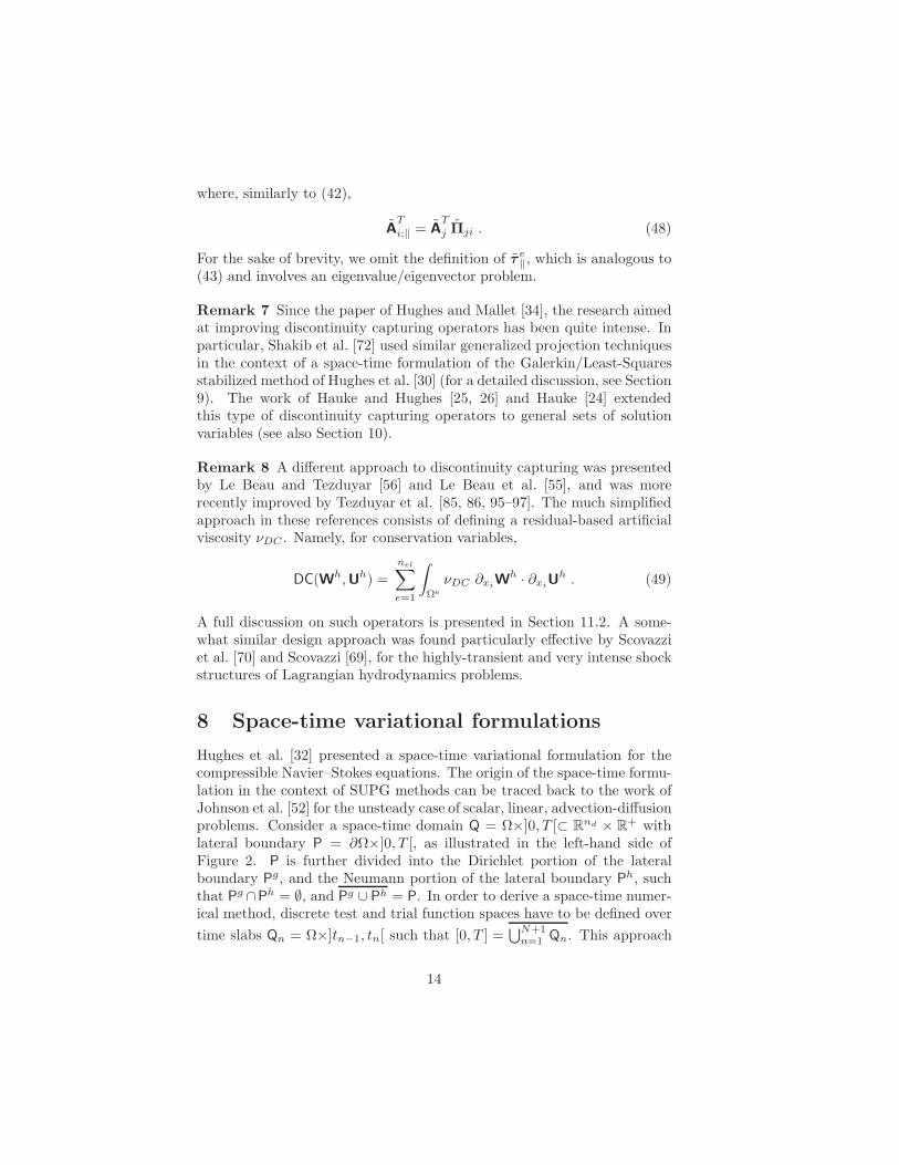
Remark 7 Since the paper of Hughes and Mallet [34], the research aimedat improving discontinuity capturing operators has been quite intense. Inparticular, Shakib et al. [72] used similar generalized projection techniquesin the context of a space-time formulation of the Galerkin/Least-Squaresstabilized method of Hughes et al. [30] (for a detailed discussion, see Section9). The work of Hauke and Hughes [25, 26] and Hauke [24] extendedthis type of discontinuity capturing operators to general sets of solutionvariables (see also Section 10).

Remark 8 A different approach to discontinuity capturing was presentedby Le Beau and Tezduyar [56] and Le Beau et al. [55], and was morerecently improved by Tezduyar et al. [85, 86, 95–97]. The much simplifiedapproach in these references consists of defining a residual-based artificialviscosity νDC . Namely, for conservation variables,

DC(Wh,Uh) =

nel∑

e=1

∫

Ωe

νDC ∂xiW

h · ∂xiU

h . (49)

A full discussion on such operators is presented in Section 11.2. A some-what similar design approach was found particularly effective by Scovazziet al. [70] and Scovazzi [69], for the highly-transient and very intense shockstructures of Lagrangian hydrodynamics problems.

8 Space-time variational formulations

Hughes et al. [32] presented a space-time variational formulation for thecompressible Navier–Stokes equations. The origin of the space-time formu-lation in the context of SUPG methods can be traced back to the work ofJohnson et al. [52] for the unsteady case of scalar, linear, advection-diffusionproblems. Consider a space-time domain Q = Ω×]0, T [⊂ R

nd × R+ with

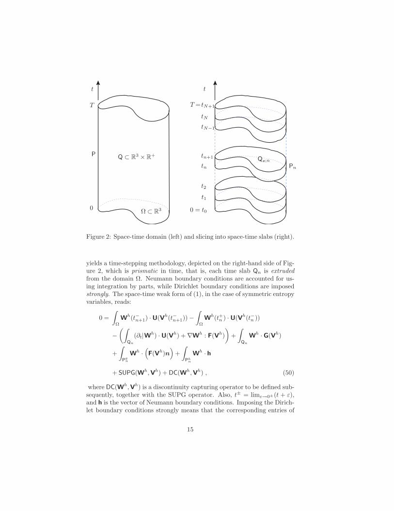
lateral boundary P = ∂Ω×]0, T [, as illustrated in the left-hand side ofFigure 2. P is further divided into the Dirichlet portion of the lateralboundary Pg, and the Neumann portion of the lateral boundary Ph, suchthat Pg ∩Ph = ∅, and Pg ∪ Ph = P. In order to derive a space-time numer-ical method, discrete test and trial function spaces have to be defined over

time slabs Qn = Ω×]tn−1, tn[ such that [0, T ] =⋃N+1

n=1 Qn. This approach

14

0 = t0

t1

t2

tn

tn+1

tN−1

tN

T = tN+1

Pn

Qx;n

Ω ⊂ R3

Q ⊂ R3 × R

+

0

T

t t

P

Figure 2: Space-time domain (left) and slicing into space-time slabs (right).

yields a time-stepping methodology, depicted on the right-hand side of Fig-ure 2, which is prismatic in time, that is, each time slab Qn is extrudedfrom the domain Ω. Neumann boundary conditions are accounted for us-ing integration by parts, while Dirichlet boundary conditions are imposedstrongly. The space-time weak form of (1), in the case of symmetric entropyvariables, reads:

0 =

∫

Ω

Wh(t−n+1) ·U(Vh(t−n+1))−

∫

Ω

Wh(t+n ) ·U(Vh(t−n ))

−

(∫

Qn

(∂t|Wh) ·U(Vh) +∇W

h : F(Vh)

)

+

∫

Qn

Wh ·G(Vh)

+

∫

Pgn

Wh ·(

F(Vh)n)

+

∫

Phn

Wh · h

+ SUPG(Wh,Vh) + DC(Wh,Vh) , (50)

where DC(Wh,Vh) is a discontinuity capturing operator to be defined sub-sequently, together with the SUPG operator. Also, t± = limε→0±(t + ε),and h is the vector of Neumann boundary conditions. Imposing the Dirich-let boundary conditions strongly means that the corresponding entries of

15

the vector Wh vanish at the Dirichlet boundary, where the boundary value

of the solution is enforced.

Remark 9 (Euler-Lagrange equations) The Euler-Lagrange equationsof the Galerkin part of the variational form (50) provide understanding ofthe nature of the variational formulation. They are obtained assumingthat the solution is sufficiently smooth, so that integration by parts can beperformed. If this is the case, (50) yields

0 =

∫

Qn

Wh ·(

∂tU(Vh) +∇· F(Vh) + Gh)

+

∫

Ω

Wh(t+n ) · [[U(Vh(tn))]]−

∫

Phn

Wh ·(

F(Vh)nx − h

)

, (51)

which enforces the Navier–Stokes equations on the interior of Qn, Neumannboundary conditions on the boundary Ph

n, initial conditions at time tn,through causality of the solution, that is, the weak continuity condition[[U(Vh(tn))]] = U(Vh(t+n ))−U(Vh(t−n )) = 0.

Remark 10 (Conservation properties) Global conservation of the for-mulation (50) is readily proved by choosing W

h constant over Qn, as-suming homogenous Neumann boundary conditions, and neglecting anysource/sink terms (Gh = 0). Hence (50) yields

∫

Ω

U(Vh(t−n+1)) =

∫

Ω

U(Vh(t−n )) , (52)

which expresses global conservation between time t−n+1 and t−n .

The first comprehensive study on space-time time integrators for the com-pressible Navier–Stokes was published in the work of Shakib and Hughes[71] and Shakib et al. [72], where first- and third-order time integratorswere analyzed and applied to a number of compressible flow computations.The first-order time integrator was obtained using a discontinuous-in-time,piecewise-constant interpolation for both the test and trial space, whilethe third-order time integrator was obtained using discontinuous-in-time,piecewise-linear interpolation. In general, a discontinuous Galerkin methodin time is of order 2k + 1, where k is the order of the interpolation.

It is also worth mentioning the fact that Petrov-Galerkin space-timeintegrators are also available, in which discontinuous polynomials of orderk are used for the test space (in time) and continuous polynomials of orderk+1 are used for the trial space (again, in time). This choice leads to meth-ods of accuracy 2k, and dates back to Hulme [42], Jamet [43], and Azizand Monk [3]. More recently, Johnson [51], French [17, 18], French and

16

Jensen [19], Estep and French [14], and French and Peterson [20] revivedthe interest in such integrators. The most common example is the methodobtained in the case k = 1, which resembles a mid-point integrator, andleads to the Crank-Nocholson method for linear problems. This approachwas successfully adopted by Scovazzi et al. [70] for explicit stabilized com-putations of Lagrangian shock-hydrodynamic flows and by Hoffman andJohnson [27] in adaptive Eulerian compressible flow computations.

9 The Galerkin/least-squares method

Hughes et al. [30] developed the Galerkin least/squares (GLS) stabilizationmethod as a generalization of the SUPG approach, and applied it to scalaradvection-diffusion problems in multiple dimensions and systems of sym-metric conservation laws. Shakib et al. [72] applied GLS to a space-timeformulation of the compressible Navier–Stokes equations, augmenting theright hand side of (52) with

SUPG(Wh,V) =

nel∑

e=1

∫

Qe

(LWh) · τ e(LVh) (53)

L = A0 ∂t + Ai ∂xi− ∂xi

(

Kij ∂xj

)

+ C (54)

τ e = A−1

0

(

C2+

(

∂ξ0

∂x0

)2

I +

(

∂ξi

∂xj

∂ξi

∂xk

)

AjAk

+

(

∂ξi

∂xk

∂ξj

∂xl

∂ξj

∂xm

∂ξi

∂xn

)

KklKmn

)(−1/2)

, (55)

and

DC(Wh,Vh) =

nel∑

e=1

∫

Qe

νDC(∇[t,ξ]Wh) · diag[A0](∇[t,ξ]V

h) , (56)

where I is the identity matrix, ξ is the coordinate in the element’s parentdomain, G

h = CVh, diag[A0] is a block-diagonal matrix in which the block

A0 is repeated as many times as necessary along the diagonal, and ∇[t,ξ] isa space-time generalized gradient which involves zeroth/first derivatives inspace and time, and second derivatives in space. For a precise definition of∇[t,ξ], the reader can refer to Shakib et al. [72], while it suffices to say thatthe proposed discontinuity capturing operator is acting along the directionof the Navier–Stokes operator, interpreted as a generalized gradient.

Remark 11 The GLS method was an important step in the developmentof stabilized methods for compressible flows since the stabilization term

17

can be proved to be strictly dissipative. This an important aspect, sincethe base Galerkin formulation augmented with the GLS term satisfies adiscrete entropy inequality, even in the inviscid limit. At the same time,when strong shocks are present, it was found important to introduce anadditional discontinuity capturing operator.

Remark 12 The expression for τ e is obtained with a methodology similarto [33] for (39), leveraging diagonalization of the Navier–Stokes system.

Remark 13 The artificial viscosity νDC is a function of appropriate normsof the residual, which yields a linear or quadratic dependence [72]. Theproposed approach stems from and extends the ideas in [34].

10 Computations with primitive variables:

Hauke and Hughes [25, 26]

During the mid-to-late 1990s, Hauke and Hughes developed compressibleSUPG formulations on sets of variables other than conservation or entropyvariables. These formulations were derived from formulations with entropyvariables, applying an additional change of variables:

A0 = A0∇YV , (57)

Ai = Ai∇YV , (58)

Kij = Kij∇YV , (59)

τe = ∇YV τ e . (60)

All the previous matrices are in general non-symmetric. Hauke and Hughes[26] compared entropy and conservation variables with density primitive

variables Y = [ρ, vT , θ]T , and pressure primitive variables Y = [p, vT , θ]T .The numerical results showed no significant differences in the case of com-pressible flow computations. However, only the pressure primitive variablesare applicable to computations in the incompressible limit, since the matrixJacobians A0, Ai, and Kij stay bounded as the speed of sound tends toinfinity.

Remark 14 Hauke and Hughes [25, 26] showed that the pressure primitivevariables were the pathway to design a generalized stabilized method, forcomputations at all Mach numbers. In this context, it is important tomention the contribution of Wong et al. [100], who proposed a scaling ofthe matrix τ

e with the Mach number, to avoid degradation of accuracy inthe nearly incompressible limit.

18

The GLS/SUPG stabilization term documented in [25, 26] reads

SUPG(Wh, Yh) =

nel∑

e=1

∫

Qen

(

LTW

h)

· τ e(LYh) , (61)

with

L = A0(Yh)∂t + Ai(Y

h)∂xi− ∂xi

(

Kij(Yh)∂xj

)

+ C , (62)

LT = AT

0 (Yh)∂t + A

T

i (Yh)∂xi− ∂xi

(

KT

ij(Yh)∂xj

)

+ CT

, (63)

where Gh = CY

h.

Remark 15 Another important contribution found in [25, 26] is the con-sistent definition of the stabilizing perturbation to the test function in thecase of non-symmetric systems. This result is obtained using the trans-formation ∇YV from entropy to non-symmetric variables, and confirms theinitial work of Tezduyar and Hughes [91, 92] and Hughes and Tezduyar[40] for conservation variables (see eq. (23)). This definition is consistentwith the the multi-scale framework (see, e.g., Hughes [28], Hughes et al.[29, 39], Scovazzi [69]).

Remark 16 In [25, 26] a simpler discontinuity capturing term DC(Wh, Yh)

was used, namely

DC(Wh, Yh) =

nel∑

e=1

∫

Ωe

νDCgij(∂xiW

h) · A0(Yh) ∂xj

Yh

, (64)

where

gij =

[

∂ξk

∂xi

∂ξk

∂xj

]−1

(65)

is the metric tensor. This definition proved robust in hypersonic computa-tions performed by Chalot and Hughes [10].

More recently Hauke [24] developed simplified forms of the stabilization anddiscontinuity capturing operators in the case of non-symmetric variables.

11 Stabilization and shock-capturing param-

eters

11.1 Stabilization parameters

For referential convenience, the original SUPG formulation of compressibleflows in conservation variables [40, 91, 92] will be called “(SUPG)82”. The

19

set of τs introduced in [40, 91, 92] in conjunction with (SUPG)82 will becalled “τ82”. The τ definition introduced in [94] automatically yields lowervalues for higher-order elements. The τ used in [56] with (SUPG)82 is aslightly modified version of τ82. The shock-capturing parameter used in[56] (defined with an expression in conservation variables, derived from theshock-capturing parameter designed for entropy variables) will be called“δ91” here. Subsequent minor modifications of τ82 took into account theinteraction between the shock-capturing and the (SUPG)82 terms in afashion similar to how it was done in [94] for advection–diffusion–reactionequations. Until recently, all these slightly modified versions of τ82 havealways been used with the same δ91, and we will categorize them here allunder the label “τ82-MOD”.

More recently, τs which are applicable to higher-order elements wereproposed in [16] in the context of advective-diffusive systems. Calculat-ing the τs based on the element-level matrices and vectors was introducedin [93] in the context of the advection–diffusion equation and the Navier–Stokes equations of incompressible flows. These definitions are expressedin terms of the ratios of the norms of the matrices or vectors. They auto-matically take into account the local length scales, advection field and theelement Reynolds number. Based on these definitions, a τ can be calculatedfor each element or for each degree-of-freedom of each element, or, as it wasproposed in [83, 87], for each integration point of each element. It was pro-posed in [84, 93] that the stabilization parameters to be used in advancingthe solution from time level n to n + 1 (including the parameter embed-ded in a stabilization term that resembles a discontinuity-capturing term)should be evaluated at time level n (i.e. based on the flow field alreadycomputed for time level n). This way we are spared from another levelof nonlinearity. The element-matrix-based τ definitions (and their degree-of-freedom versions) introduced in [93] were applied in [7] (and in [8]) to(SUPG)82, supplemented with the shock-capturing term with δ91.

Various options for calculating the stabilization parameters in the con-text of the (SUPG)82 formulation were introduced in [85, 86]. In thissection we describe those options. For this purpose, we first define theacoustic speed as c, and define the unit vector j as

j =∇ρh

‖ ∇ρh ‖. (66)

In computing τSUGN1 (advection-dominated limit of the stabilization param-eter we are starting to define) for each component of the test vector-functionW

h, the stabilization parameters τρSUGN1, τu

SUGN1 and τeSUGN1 (associated

with the mass, momentum and energy balance equations) are defined by

20

the following expression:

τρSUGN1 = τu

SUGN1 = τeSUGN1 =

(

nen∑

a=1

(

c |j · ∇Na|+ |vh · ∇Na|

)

)−1

. (67)

where nen is the number of element nodes, vh is the flow velocity, andNa is the shape functions associated with node a. In computing τSUGN2

(transient-dominated limit), the parameters τρSUGN2, τu

SUGN2 and τeSUGN2

are defined as follows:

τρSUGN2 = τu

SUGN2 = τeSUGN2 =

∆t

2. (68)

In computing τSUGN3 (diffusion-dominated limit), the parameter τuSUGN3 is

defined by using the expression

τuSUGN3 =

h2RGN

4ν, (69)

where

hRGN = 2

(

nen∑

a=1

|r · ∇Na|

)−1

, r =∇‖vh‖

‖ ∇‖vh‖ ‖. (70)

The parameter τeSUGN3 is defined as

τeSUGN3 =

(heRGN)2

4κe, (71)

where

heRGN = 2

(

nen∑

a=1

|re · ∇Na|

)−1

, re =∇θh

‖ ∇θh ‖. (72)

The parameters (τρSUPG)UGN, (τu

SUPG)UGN and (τe

SUPG)UGN are calculated from

their components by using the “r-switch” [93]:

(τρSUPG)UGN =

(

1

(τρSUGN1)r

+1

(τρSUGN2)r

)− 1r

, (73)

(τuSUPG)UGN =

(

1

(τuSUGN1)r

+1

(τuSUGN2)r

+1

(τuSUGN3)r

)− 1r

, (74)

(τeSUPG)UGN =

(

1

(τeSUGN1)r

+1

(τeSUGN2)r

+1

(τeSUGN3)r

)− 1r

, (75)

where, typically, r = 2.

21

11.2 New shock-capturing technology and the Y Zβ ap-proach

In the context of shock-capturing, the Discontinuity-Capturing DirectionalDissipation (DCDD) stabilization was introduced in [82, 84] for incom-pressible flows with sharp gradients. The DCDD takes effect where thereis a sharp gradient in the velocity field and introduces dissipation in thedirection of that gradient. The way the DCDD is added to the formula-tion precludes augmentation of the SUPG effect by the DCDD effect whenthe advection and discontinuity directions coincide. The DCDD involvesa second element length scale, which was also introduced in [82, 84] andis based on the solution gradient. This new element length scale is usedtogether with the element length scales defined earlier in [94]. Recognizingthis second element length as a diffusion length scale, new stabilizationparameters for the diffusive limit were introduced for incompressible flowsin [84, 86]. Partly based on the ideas underlying the new τs for incom-pressible flows, new ways of calculating the τs for compressible flows wereintroduced in [85, 86], and these new stabilization parameters were re-viewed in Section 11.1. More significantly, new ways of calculating theshock-capturing parameters for compressible flows were also introducedin [86]. The objective was to have shock-capturing parameters that aresimpler, and less costly to compute with, than δ91. Some versions of thesenew shock-capturing parameters are based on ideas underlying the DCDD.Other versions, which were categorized as “Y Zβ Shock-Capturing”, arebased on scaled residuals and are defined with options for smoother orsharper shocks. This approach is described next.

First, the “shock-capturing viscosity” νSHOC is defined as

νSHOC =∥

∥Y−1

Z∥

∥

(

nd∑

i=1

∥

∥

∥Y

−1∂xiU

h∥

∥

∥

2)β/2−1

(

hSHOC

2

)β

, (76)

where Y is a diagonal scaling matrix constructed from the reference valuesof the components of U:

Y =

(U1)ref 0 0 0 00 (U2)ref 0 0 00 0 (U3)ref 0 00 0 0 (U4)ref 00 0 0 0 (U5)ref

, (77)

Z = ∂tUh + Ai∂xi

Uh (78)

or

Z = Ahi ∂xi

Uh (79)

22

and

hSHOC = hJGN , (80)

hJGN = 2

(

nen∑

a=1

|j · ∇Na|

)−1

. (81)

The parameter β is set as β = 1 for smoother shocks and β = 2 for sharpershocks. In a variation of the expression given by Eq. (76), νSHOC is definedby the following expression:

νSHOC =∥

∥Y−1

Z∥

∥

(

nd∑

i=1

∥

∥

∥Y

−1∂xiU

h∥

∥

∥

2)β/2−1

∥

∥

∥Y

−1U

h∥

∥

∥

1−β(

hSHOC

2

)β

. (82)

The compromise between the β = 1 and β = 2 selections is defined as thefollowing averaged expression for νSHOC :

νSHOC =1

2

(

(νSHOC)β=1 + (νSHOC)β=2

)

. (83)

Versions of νSHOC that take into account the Mach number and shock in-tensity across a shock was proposed in [96, 97]. In that, νSHOC given byEqs. (76) and (82) are modified as follows:

νSHOC ← νSHOC

(

1 +

(

‖ ∇ρh ‖ hSHOC

ρref

)

< M1/bM − 1 >

)2/bF

, (84)

where M is the Mach number and “< · · · >” is the Macaulay bracket:

< x− y > =

0, x ≤ yx− y, x > y

. (85)

The reference density ρref is defined as

ρref = ρinf

(

ρsca

ρinf

)bR/2

, (86)

where ρinf is the density at the inflow and ρsca is a scaling density. In defin-ing ρsca, one of the options we consider is ρsca = ρinf. For flows with shocks,we also consider the options ρsca = ρ2 and ρsca = ρ2 − ρ1, where ρ1 andρ2 are the density values before and after a normal shock correspondingto the inflow Mach number. The parameters bM, bF and bR can each beset to 1 for smoother shocks and 2 for sharper shocks. Eq. (84), withoutthe exponent 2/bF, was originally introduced in [96]. With this expression,

23

the definition of the shock-capturing viscosity takes into account the Machnumber and shock intensity across a shock. The shock intensity is repre-

sented by the term(

‖ ∇ρh ‖ hSHOC

ρref

)

, which is a scaled measure of the jump

in density. The Mach number is represented by the term < M1/bM − 1 >,which becomes active for M > 1.

Based on Eq. (76), a separate νSHOC can be calculated for each compo-nent of the test vector-function W

h:

(νSHOC)I =∣

∣

(

Y−1

Z)

I

∣

∣

(

nd∑

i=1

∣

∣

∣

(

Y−1∂xi

Uh)

I

∣

∣

∣

2)β/2−1

(

hSHOC

2

)β

, I = 1, 2, . . . nd + 2. (87)

Similarly, a separate νSHOC for each component of Wh can be calculated

based on Eq. (82):

(νSHOC)I =∣

∣

(

Y−1

Z)

I

∣

∣

(

nd∑

i=1

∣

∣

∣

(

Y−1∂xi

Uh)

I

∣

∣

∣

2)β/2−1

∣

∣

∣

(

Y−1

Uh)

I

∣

∣

∣

1−β

(

hSHOC

2

)β

, I = 1, 2, . . . nd + 2. (88)

Given νSHOC, the shock-capturing term is defined as

SSHOC =

nel∑

e=1

∫

Ωe

∇Wh :(

κκκSHOC · ∇Uh)

dΩ , (89)

where κκκSHOC is defined as κκκSHOC = νSHOC I. As a possible alternative, it isdefined as κκκSHOC = νSHOC jj. If the option given by Eq. (87) or Eq. (88)is exercised, then νSHOC becomes an (nd + 2) × (nd + 2) diagonal matrix,and the matrix κκκSHOC becomes augmented from an nd × nd matrix to an(nd × (nd + 2))× ((nd + 2)× nd) matrix.

To preclude compounding, νSHOC can be modified as follows:

νSHOC ← νSHOC − switch(

τSUPG

(

j · vh)2

, τSUPG

(

|j · vh| − c)2

, νSHOC

)

, (90)

where the “switch” function is defined as the “min” function or as the“r-switch” used earlier in this section. For viscous flows, the above modifi-cation would be made separately with each of τρ

SUPG, τuSUPG and τe

SUPG, andthis would result in νSHOC becoming a diagonal matrix even if the optiongiven by Eq. (87) or Eq. (88) is not exercised.

24

A preliminary set of test computations with these new shock-capturingparameters were reported in [95] for inviscid supersonic flows. Those com-putations were limited to very simple 2D geometries and quadrilateralelements. A more comprehensive set of 2D test computations for invis-cid supersonic flows were reported in [96]. Those tests with the Y Zβshock-capturing involved different element types and mesh orientations.In [97], numerical experiments were carried out for inviscid supersonicflows around cylinders and spheres to evaluate the performance of the Y Zβshock-capturing in more challenging test problems. In those numerical ex-periments, in addition to comparing the Y Zβ results to those obtainedwith δ91, for 2D structured meshes, the Y Zβ result were compared to theresults obtained with the OVERFLOW code [6]. All these test compu-tations showed that, these new shock-capturing parameters are not onlymuch simpler than δ91, but also superior in accuracy.

In [66], the Y Zβ shock-capturing was used in combination with theVariable Subgrid Scale (V-SGS) method, which was formulated for com-pressible flows in conservation variables in [65]. The V-SGS method wasfirst introduced in [12] for the advection–diffusion–reaction equation andfor incompressible flows. It is based on an approximation of the classof SGS models derived from the Hughes Variational Multiscale (Hughes-VMS) method [28]. The results reported in [66] show that the Y Zβ shock-capturing yields better performance also when it is used in conjunctionwith the V-SGS method.

12 Stabilized ALE methods

Stabilized methods for compressible flows on arbitrary Lagrangian-Eulerian(ALE) meshes were initially developed by Masud [58], Rifai et al. [62, 63],for various engineering applications, among which fluid/structure interac-tion problems. These methods are easily implemented by modifying theadvective flux F

(c) in (7) as follows:

F(c) = U⊗ c , (91)

where c = v − v is the convective velocity across the moving mesh andv is the mesh velocity. The stabilization operators have to be modifiedaccordingly.

Remark 17 The ALE framework is useful for the design of stabilizedmethods in their most general form, and was recently adopted by Scov-azzi [67] and Scovazzi [68] to study the Galilean invariance properties ofSUPG operators.

25

13 Stabilized Lagrangian methods

Scovazzi et al. [70] and Scovazzi [69] successfully developed SUPG-stabilizedmethods for compressible hydrodynamics computations (characterized byhighly unsteady flows with Mach numbers in excess of 103) on Lagrangianmeshes (i.e., c = 0). Algorithms of shock hydrodynamics (hydrocodesin short) are traditionally developed on quadrilaterals/hexahedral meshesand, because of the piecewise-constant discretization of the thermodynamicfields, have never been successfully generalized to triangular/tetrahedralmeshes. The advantage of using simplex-type meshes is evident in terms ofautomatic mesh generation, multi-material interface reconstruction, multi-physics radiation-hydrodynamics applications.

The methodology developed in [70] represented the first example ofaccurate and robust computations on simplex-type meshes of shock hydro-dynamic flows, with comparable and sometimes superior quality to state-of-the-art hydrocodes on brick meshes. This approach is significantly differentfrom mainstream stabilized methods for compressible flows, and the readeris prompted to see [69, 70] for specific details. A brief description of themain features is presented next:

1. The set of solution variables is given by the vector Y = [ρ, vT , p]T .

2. An explicit predictor-multicorrector approach is adopted, since hy-drocodes typically involve explicit time integration. The time integra-tor is the second-order space-time Petrov-Galerkin method describedat the end of Section 8, and involves piecewise-linear, continuous trialfunctions in time, and piecewise-constant, discontinuous test func-tions in time. This methodology provides more compact storage andless computational burden with respect to the third-order algorithmproposed in [72].

3. To enhance performance and avoid either inverting matrices or solv-ing eigenvalue/eigenvector problems on each element, a very simplediagonal matrix τ is used. Variational multi-scale interpretations areembedded in the proposed design for τ [69]. This simple appraochperformed very well in highly transient flows.

4. The discontinuity operator was designed as an isotropic Laplace op-erator acting on the current configuration gradients of the solution.This property was found very important in the solution of highly tran-sient shock waves. The structure of the artificial-viscosity/discontinuity-capturing operator is isotropic in space, and somewhat similar to theY Zβ approach and (49).

26

5. In addition, and differently from any other discontinuity capturingapproach in SUPG methods, the work done by the artificial stresseswas introduced in the energy equation: This term was found crucialin the solution of piston-driven shock-wave problems.

14 Compressible turbulence

Compressible turbulence computations using pressure primitive variableswere studied by Jansen et al. [46] and Jansen [44], where κ− ε turbulencemodels were used to provide a cost-effective computational procedure. Inlater work of Hughes et al. [36, 37, 38], the variational multi-scale paradigmwas used to provide a large eddy simulation (LES) model of turbulence,and was later incorporated by Whiting et al. [99] in a stabilized finiteelement method for compressible flows. Jansen et al. [47] also developedgeneralized-α time integrators for compressible turbulence computations,with improved high-frequency dissipation.

At the same time, Corsini et al. [13], Rispoli et al. [64] developed anumber of residual-based eddy viscosity LES models aimed at stabilizedcompressible computations of turbo-machinery flows. The key idea in thiswork is the realization that a residual-based eddy viscosity dynamicallyadjusts to the conditions of the turbulent flow, and switches off for smooth(laminar) flow.

15 Summary

We reviewed 25 years of work on stabilized methods for compressible flows.We presented a unified view by tracking over time the main ideas thatinfluenced the field, and by showing how these ideas evolved within thedifferent research groups, from the origins until present times.

Acknowledgements

T.J.R. Hughes was partially supported by Sandia National Laboratoriesunder Contract No. 114166. G. Scovazzi was partially funded by the DOENNSA Advanced Scientific Computing Program and the Computer ScienceResearch Institute (CSRI) at Sandia National Laboratories. T.E. Tezduyarwas partially supported by NASA Johnson Space Center under Grant No.NAG9-1435. These sources of support are gratefully acknowledged by theauthors.

27

References

[1] Aliabadi, S. K., Ray, S. E., and Tezduyar, T. E. (1993). SUPG finiteelement computation of compressible flows with the entropy and conser-vation variables formulations. Computational Mechanics, 11:300–312.

[2] Aliabadi, S. K. and Tezduyar, T. E. (1993). Space–time finite ele-ment computation of compressible flows involving moving boundariesand interfaces. Computer Methods in Applied Mechanics and Engineer-ing, 107(1–2):209–223.

[3] Aziz, A. K. and Monk, P. (1989). Continuous finite elements in spaceand time for the heat equation. Mathematics of Computation, 52:255–274.

[4] Baba, K. and Tabata, M. (1981). On a conservative upwind finite ele-ment scheme for the convective diffusion equations. R.A.I.R.O., AnalyseNumerique, 27:277–282.

[5] Brooks, A. N. and Hughes, T. J. R. (1982). Streamline upwind /Petrov-Galerkin formulations for convection dominated flows with par-ticular emphasis on the incompressible Navier-Stokes equations. Com-puter Methods in Applied Mechanics and Engineering, 32:199–259.

[6] Buning, P. G., Jespersen, D. C., Pulliam, T. H., Klopfer, G. H., Chan,W. M., Slotnick, J. P., Krist, S. E., and Renze, K. J. (2000). OVER-FLOW User’s Manual, Version 1.8s, 28 November 2000. NASA LangleyResearch Center, Hampton, Virginia.

[7] Catabriga, L., Coutinho, A. L. G. A., and Tezduyar, T. E. (2005).Compressible flow SUPG parameters computed from element matrices.Communications in Numerical Methods in Engineering, 21:465–476.

[8] Catabriga, L., Coutinho, A. L. G. A., and Tezduyar, T. E. (2006).Compressible flow supg parameters computed from degree-of-freedomsubmatrices. Computational Mechanics, 38:334–343.

[9] Chalot, F. E. (2004). Industrial aerodynamics. In Stein, E., de Borst,R., and Hughes, T. J. R., editors, Encyclopedia of Computational Me-chanics. John Wiley & Sons.

[10] Chalot, F. E. and Hughes, T. J. R. (1994). A consistent equilibriumchemistry algorithm for hypersonic flows. Computer Methods in AppliedMechanics and Engineering, 112:25–40.

28

[11] Christie, I., Griffiths, D. F., and Sanz-Serna, J. M. (1981). Productapproximantion for non-linear problems in the finite element method.IMA Journal on Numerical Analysis, 1:253–266.

[12] Corsini, A., Rispoli, F., and Santoriello, A. (2005). A variationalmultiscale high-order finite element formulation for turbomachinery flowcomputations. Computer Methods in Applied Mechanics and Engineer-ing, 194:4797–4823.

[13] Corsini, A., Rispoli, F., Santoriello, A., and Tezduyar, T. E. (2006).Improved discontinuity-capturing finite element techniques for reactioneffects in turbulence computation. Computational Mechanics, 38:356–364.

[14] Estep, D. and French, D. A. (1994). Global error control for the contin-uous Galerkin finite element method for ordinary differential equations.R.A.I.R.O., 28:815–852.

[15] Fletcher, C. A. (1983). The group finite element formulation. Com-puter Methods in Applied Mechanics and Engineering, 37(2):225–244.

[16] Franca, L. P., Frey, S. L., and Hughes, T. J. R. (1992). Stabilizedfinite element methods: I. Application to the advective-diffusive model.Computer Methods in Applied Mechanics and Engineering, 95:253–276.

[17] French, D. A. (1993). A space-time finite element method for the waveequation. Computer Methods in Applied Mechanics and Engineering,107:145–157.

[18] French, D. A. (1999). Continuous Galerkin finite element methodsfor a forward-backward heat equation. Numerical Methods for PartialDifferential Equations, 15:491–506.

[19] French, D. A. and Jensen, S. (1994). Long time behaviour of arbitraryorder continuous time Galerkin schemes for some one-dimensional phasetransition problems. IMA Journal on Numerical Analysis, 14:421–442.

[20] French, D. A. and Peterson, T. E. (1996). A continuous space-timefinite element method for the wave equation. Mathematics of Computa-tion, 65:491–506.

[21] Godunov, S. K. (1961). An interesting class of quasilinear systems.Dokl. Akad. Nauk. SSSR, 139:521–523.

[22] Harten, A. (1983). On the symmetric form of systems of conservationlaws with entropy. Journal of Computational Physics, 49:151–164.

29

[23] Hauke, G. (1995). A unified approach to compressible and incompress-ible flows and a new entropy-consistent formulation of the κ-ε model.PhD thesis, Mechanical Engineering Department, Stanford University.

[24] Hauke, G. (2001). Simple stabilizing matrices for the computation ofcompressible flows in primitive variables. Computer Methods in AppliedMechanics and Engineering, 190:6881–6893.

[25] Hauke, G. and Hughes, T. J. R. (1994). A unified approach to com-pressible and incompressible flows. Computer Methods in Applied Me-chanics and Engineering, 113:389–396.

[26] Hauke, G. and Hughes, T. J. R. (1998). A comparative study ofdifferent sets of variables for solving compressible and incompressibleflows. Computer Methods in Applied Mechanics and Engineering, 153:1–44.

[27] Hoffman, J. and Johnson, C. (2004). Computability and adaptivity incfd. In Stein, E., de Borst, R., and Hughes, T. J. R., editors, Encyclopediaof Computational Mechanics. John Wiley & Sons.

[28] Hughes, T. J. R. (1995). Multiscale phenomena: Green’s functions, theDirichlet-to-Neumann formulation, subgrid-scale models, bubbles andthe origin of stabilized methods. Computer Methods in Applied Mechan-ics and Engineering, 127:387–401.

[29] Hughes, T. J. R., Feijoo, G., Mazzei, L., and Quincy, J.-B. (1998).The Variational Multiscale Method — a paradigm for computationalmechanics. Computer Methods in Applied Mechanics and Engineering,166:3–24.

[30] Hughes, T. J. R., Franca, L. P., and Hulbert, G. M. (1989). A newfinite element formulation for computational fluid dynamics: VIII. TheGalerkin/least-squares method for advective-diffusive equations. Com-puter Methods in Applied Mechanics and Engineering, 73:173–189.

[31] Hughes, T. J. R., Franca, L. P., and Mallet, M. (1986a). A new fi-nite element formulation for computational fluid dynamics: I. Symmetricforms of the compressible Euler and Navier-Stokes equations and the sec-ond law of thermodynamics. Computer Methods in Applied Mechanicsand Engineering, 54:223–234.

[32] Hughes, T. J. R., Franca, L. P., and Mallet, M. (1987). A new finiteelement formulation for computational fluid dynamics: VI. Convergenceanalysis of the generalized SUPG formulation for linear time-dependentmultidimensional advective-diffusive systems. Computer Methods in Ap-plied Mechanics and Engineering, 63:97–112.

30

[33] Hughes, T. J. R. and Mallet, M. (1986a). A new finite element for-mulation for computational fluid dynamics: III. The generalized stream-line operator for multidimensional advective-diffusive systems. ComputerMethods in Applied Mechanics and Engineering, 58:305–328.

[34] Hughes, T. J. R. and Mallet, M. (1986b). A new finite element formu-lation for computational fluid dynamics: IV. A discontinuity-capturingoperator for multidimensional advective-diffusive systems. ComputerMethods in Applied Mechanics and Engineering, 58:329–336.

[35] Hughes, T. J. R., Mallet, M., and Mizukami, A. (1986b). A newfinite element formulation for computational fluid dynamics: II. Be-yond SUPG. Computer Methods in Applied Mechanics and Engineering,54:341–355.

[36] Hughes, T. J. R., Mazzei, L., and Jensen, K. E. (2000). Large eddysimulation and the variational multiscale method. Computing and Visu-alization in Science, 3(47):147–162.

[37] Hughes, T. J. R., Mazzei, L., Oberai, A. A., and Wray, A. (2001a). Themultiscale formulation of large eddy simulation: decay of homogenousisotropic turbulence. Physics of Fluids, 13:505–512.

[38] Hughes, T. J. R., Oberai, A. A., and Mazzei, L. (2001b). Largeeddy simulation of turbulent channel flows by the variational multiscalemethod. Physics of Fluids, 13(6):1784–1799.

[39] Hughes, T. J. R., Scovazzi, G., and Franca, L. P. (2004). Multiscaleand stabilized methods. In Stein, E., de Borst, R., and Hughes, T. J. R.,editors, Encyclopedia of Computational Mechanics. John Wiley & Sons.

[40] Hughes, T. J. R. and Tezduyar, T. E. (1984). Finite element methodsfor first-order hyperbolic systems with particular emphasis on the com-pressible Euler equations. Computer Methods in Applied Mechanics andEngineering, 45:217–284.

[41] Hughes, T. J. R., Winget, J., Levit, I., and Tezduyar, T. E. (1983).New alternating direction procedures in finite element analysis basedupon EBE approximate factorizations. In Atluri, S. and Perrone, N., ed-itors, Computer Methods for Nonlinear Solids and Structural Mechanics,AMD-Vol.54, pages 75–109. ASME, New York.

[42] Hulme, B. L. (1972). Discrete Galerkin and related one-step methodsfor ordinary differential equations. Mathematics of Computation, 26-120:881–891.

31

[43] Jamet, P. (1980). Stability and convergence of a generalized Crank-Nicolson scheme on a variable mesh for the heat equation. SIAM Journalon Numerical Analysis, 17(4):530–539.

[44] Jansen, K. E. (1999). A stabilized finite element method for computingturbulence. Computer Methods in Applied Mechanics and Engineering,174:299–317.

[45] Jansen, K. E. and Hughes, T. J. R. (1995). A stabilized finite elementmethod for the Reynolds-averaged Navier-Stokes equations. Surveys onMathematics for Industry, 4:279–317.

[46] Jansen, K. E., Johan, Z., and Hughes, T. J. R. (1993). Implementationof a one-equation turbulence model within a stabilized finite element for-mulation of a symmetric advective-diffusive system. Computer Methodsin Applied Mechanics and Engineering, 105:405–433.

[47] Jansen, K. E., Whiting, C. H., and Hulbert, G. M. (2000). Ageneralized-α method for integrating the filtered Navier-Stokes equationswith a stabilized finite element method. Computer Methods in AppliedMechanics and Engineering, 190:305–319.

[48] Johan, Z., Mathur, K. K., Johonsson, S. L., and Hughes, T. J. R.(1992). A data parallel finite element method for computational fluiddynamics on the Connection Machine system . Computer Methods inApplied Mechanics and Engineering, 99:113–134.

[49] Johan, Z., Mathur, K. K., Johonsson, S. L., and Hughes, T. J. R.(1994a). An efficient communications strategy for finite element methodson the Connection Machine CM-5 system. Computer Methods in AppliedMechanics and Engineering, 113:363–387.

[50] Johan, Z., Mathur, K. K., Johonsson, S. L., and Hughes, T. J. R.(1994b). Scalability of finite element applications on distributed-memoryparallel computers. Computer Methods in Applied Mechanics and Engi-neering, 119:61–72.

[51] Johnson, C. (1993). Discontinuous Galerkin finite element methodsfor second order hyperbolic problems. Computer Methods in AppliedMechanics and Engineering, 107:117–129.

[52] Johnson, C., Navert, U., and Pitkaranta, J. (1984). Finite elementmethods for linear hyperbolic problems. Computer Methods in AppliedMechanics and Engineering, 45:285–312.

32

[53] Johnson, C. and Szepessy, A. (1987). On the convergence of a finite el-ement method for a nonlinear hyperbolic conservation law. Mathematicsof Computation, 49:427–444.

[54] Johnson, C., Szepessy, A., and Hansbo, P. (1990). On the conver-gence of shock-capturing streamline diffusion finite element methods forhyperbolic conservation laws. Mathematics of Computation, 54:107–129.

[55] Le Beau, G. J., Ray, S. E., Aliabadi, S. K., and Tezduyar, T. E. (1993).SUPG finite element computation of compressible flows with the entropyand conservation variables formulations. Computer Methods in AppliedMechanics and Engineering, 104:397–422.

[56] Le Beau, G. J. and Tezduyar, T. E. (1991a). Finite element computa-tion of compressible flows with the SUPG formulation. In Advances inFinite Element Analysis in Fluid Dynamics, FED-Vol.123, pages 21–27,New York. ASME.

[57] Le Beau, G. J. and Tezduyar, T. E. (1991b). Finite element solutionof flow problems with mixed-time integration. Journal of EngineeringMechanics, 117:1311–1330.

[58] Masud, A. (2006). Effects of mesh motion on the stability and con-vergence of ALE based formulations for moving boundary flows. Com-putational Mechanics, 38(4-5):430–439.

[59] Mittal, S., Aliabadi, S., and Tezduyar, T. (1999). Parallel computa-tion of unsteady compressible flows with the EDICT. ComputationalMechanics, 23:151–157.

[60] Mittal, S. and Tezduyar, T. (1998). A unified finite element formu-lation for compressible and incompressible flows using augumented con-servation variables. Computer Methods in Applied Mechanics and Engi-neering, 161:229–243.

[61] Moch, M. S. (1980). Systems of conservation laws of mixed type.Journal of Differential Equations, 37:70–88.

[62] Rifai, S. M., Buell, J. C., Johan, Z., and Hughes, T. J. R. (2000). Auto-motive design applications of fluid flow simulation on parallel computingplatforms. Computer Methods in Applied Mechanics and Engineering,184:449–466.

[63] Rifai, S. M., Johan, Z., Wang, W.-P., Grisval, J.-P., Hughes, T. J. R.,and Ferencz, R. M. (1999). Multiphysics simulation of flow-induced vi-brations and aeroelasticity on parallel computing platforms. ComputerMethods in Applied Mechanics and Engineering, 174:393–417.

33

[64] Rispoli, F., Corsini, A., and Tezduyar, T. E. (2007a). Finite elementcomputation of turbulent flows with the discontinuity-capturing direc-tional dissipation (DCDD). Computers and Fluids, 36:121–126.

[65] Rispoli, F. and Saavedra, R. (2006). A stabilized finite element methodbased on SGS models for compressible flows. Computer Methods in Ap-plied Mechanics and Engineering, 196:652–664.

[66] Rispoli, F., Saavedra, R., Corsini, A., and Tezduyar, T. E. (2007b).Computation of inviscid compressible flows with the V-SGS stabilizationand YZβ shock-capturing. International Journal for Numerical Methodsin Fluids, 54:695–706.

[67] Scovazzi, G. (2007a). A discourse on Galilean invariance and SUPG-type stabilization. Computer Methods in Applied Mechanics and Engi-neering, 196(4–6):1108–1132.

[68] Scovazzi, G. (2007b). Galilean invariance and stabilized methods forcompressible flows. International Journal for Numerical Methods in Flu-ids, 54(6–8):757–778.

[69] Scovazzi, G. (2007c). Stabilized shock hydrodynamics: II. Design andphysical interpretation of the SUPG operator for Lagrangian computa-tions. Computer Methods in Applied Mechanics and Engineering, 196(4–6):966–978.

[70] Scovazzi, G., Christon, M. A., Hughes, T. J. R., and Shadid, J. N.(2007). Stabilized shock hydrodynamics: I. A Lagrangian method. Com-puter Methods in Applied Mechanics and Engineering, 196(4–6):923–966.

[71] Shakib, F. and Hughes, T. J. R. (1991). A new finite element formu-lation for computational fluid dynamics: IX. Fourier analysis of space-time Galerkin/least-squares algorithms. Computer Methods in AppliedMechanics and Engineering, 87:35–58.

[72] Shakib, F., Hughes, T. J. R., and Johan, Z. (1991). A new finite el-ement formulation for computational fluid dynamics: X. The compress-ible Euler and Navier-Stokes equations. Computer Methods in AppliedMechanics and Engineering, 89:141–219.

[73] Spradley, L. W., Stalnaker, J. F., and Ratliff, A. W. (1980). Compu-tation of three-dimensional viscous flows with the Navier-Stokes equa-tions. AIAA-80-1348. AIAA 13th Fluid and Plasma Dynamics Confer-ence, Snowmass, Colorado.

34

[74] Szepessy, A. (1989). Convergence of a shock-capturing streamline dif-fusion finite element method for a scalar conservation law in two spacedimensions. Mathematics of Computation, 53:527–545.

[75] Tabata, M. (1977). A finite element approximation corrrespondingto the upwind finite differencing. Memoirs of Numerical Mathematics,4:47–63.

[76] Tabata, M. (1978). Uniform convergence of the upwind finite elementapproximation for semilinear parabolic problems. Journal of Mathemat-ics of Kyoto University, 18:327–351.

[77] Tabata, M. (1979). Some applications of the upwind finite elementmethod. Theoretical and Applied Mechanics, 27:277–282.

[78] Tabata, M. (1985). Symmetric finite element approximations forconvection-diffusion problems. Theoretical and Applied Mechanics,33:445–453.

[79] Tezduyar, T., Aliabadi, S., Behr, M., Johnson, A., Kalro, V., andLitke, M. (1996). Flow simulation and high performance computing.Computational Mechanics, 18:397–412.

[80] Tezduyar, T., Aliabadi, S., Behr, M., Johnson, A., and Mittal, S.(1993). Parallel finite-element computation of 3D flows. Computer,26(10):27–36.

[81] Tezduyar, T. E. (1992). Stabilized finite element formulations for in-compressible flow computations. Advances in Applied Mechanics, 28:1–44.

[82] Tezduyar, T. E. (2001). Adaptive determination of the finite elementstabilization parameters. In Proceedings of the ECCOMAS Computa-tional Fluid Dynamics Conference 2001 (CD-ROM), Swansea, Wales,United Kingdom.

[83] Tezduyar, T. E. (2002). Calculation of the stabilization parametersin SUPG and PSPG formulations. In Proceedings of the First South-American Congress on Computational Mechanics (CD-ROM), Santa Fe–Parana, Argentina.

[84] Tezduyar, T. E. (2003). Computation of moving boundaries and inter-faces and stabilization parameters. International Journal for NumericalMethods in Fluids, 43:555–575.

35

[85] Tezduyar, T. E. (2004a). Determination of the stabilization and shock-capturing parameters in SUPG formulation of compressible flows. InProceedings of European Congress on Computational Methods in AppliedSciences and Engineering ECCOMAS 2004, Jyaskyla, Finland.

[86] Tezduyar, T. E. (2004b). Finite element methods for fluid dynamicswith moving boundaries and iterfaces. In Stein, E., de Borst, R., andHughes, T. J. R., editors, Encyclopedia of Computational Mechanics,Volume 3: Fluids, chapter 17. John Wiley & Sons.

[87] Tezduyar, T. E. (2005). Calculation of the stabilization parameters infinite element formulations of flow problems. In Idelsohn, S. and Son-zogni, V., editors, Applications of Computational Mechanics in Struc-tures and Fluids, pages 1–19. CIMNE, Barcelona, Spain.

[88] Tezduyar, T. E., Aliabadi, S. K., Behr, M., and Mittal, S. (1994). Mas-sively parallel finite element simulation of compressible and incompress-ible flows. Computer Methods in Applied Mechanics and Engineering,119:157–177.

[89] Tezduyar, T. E., Behr, M., and Liou, J. (1992a). A new strategy forfinite element computations involving moving boundaries and interfaces– The deforming-spatial-domain/space-time procedure: I. The conceptand the preliminary numerical tests. Computer Methods in Applied Me-chanics and Engineering, 94:339–351.

[90] Tezduyar, T. E., Behr, M., Mittal, S., and Liou, J. (1992b). A newstrategy for finite element computations involving moving boundariesand interfaces – The deforming-spatial-domain/space-time procedure:II. Computation of free-surface flows, two-liquid flows, and flows withdrifting cylinders. Computer Methods in Applied Mechanics and Engi-neering, 94:353–371.

[91] Tezduyar, T. E. and Hughes, T. J. R. (1982). Developmentof time-accurate finite element techniques for first-order hyper-bolic systems with particular emphasis on the compressible Eulerequations. NASA Technical Report NASA-CR-204772, NASA.http://ntrs.nasa.gov/archive/nasa/casi.ntrs.nasa.gov/19970023187 1997034954.pdf.

[92] Tezduyar, T. E. and Hughes, T. J. R. (1983). Finite element formu-lations for convection dominated flows with particular emphasis on thecompressible Euler equations. In Proceedings of AIAA 21st AerospaceSciences Meeting, AIAA Paper 83-0125, Reno, Nevada.

[93] Tezduyar, T. E. and Osawa, Y. (2000). Finite element stabilizationparameters computed from element matrices and vectors. ComputerMethods in Applied Mechanics and Engineering, 190:411–430.

36

[94] Tezduyar, T. E. and Park, Y. J. (1986). Discontinuity capturingfinite element formulations for nonlinear convection-diffusion-reactionequations. Computer Methods in Applied Mechanics and Engineering,59:307–325.

[95] Tezduyar, T. E. and Senga, M. (2006). Stabilization and shock-capturing parameters in SUPG formulation of compressible flows. Com-puter Methods in Applied Mechanics and Engineering, 195:1621–1632.

[96] Tezduyar, T. E. and Senga, M. (2007). SUPG finite element computa-tion of inviscid supersonic flows with YZβ shock-capturing. Computers& Fluids, 36:147–159.

[97] Tezduyar, T. E., Senga, M., and Vicker, D. (2006). Computation ofinviscid supersonic flows around cylinders and spheres with the supg for-mulation and YZβ shock-capturing. Computational Mechanics, 38:469–481.

[98] Venkatakrishnan, V., Allmaras, S., Kamenetskii, D., and Johnson, F.(June 23-26, 2003). Higher order schemes for the compressible Navier-Stokes equations. AIAA 2003-3987. AIAA 16th Computational FluidDynamics Conference, Orlando, Florida.

[99] Whiting, C. H., Jansen, K. E., and Dey, S. (2003). Hierarchical basisfor stabilized finite element methods for compressible flows. ComputerMethods in Applied Mechanics and Engineering, 192:5167–5185.

[100] Wong, J. S., Darmofal, D. L., and Peraire, J. (2001). The solution ofthe compressible Euler equation at low Mach numbers using a stabilizedfinite element algorithm. Computer Methods in Applied Mechanics andEngineering, 190:5719–5737.

37