tutorial 3. modeling external compressible flonwb/lectures/goodpracticecfd/articles/tut03...tutorial...
TRANSCRIPT
Tutorial 3. Modeling External Compressible Flow
Introduction
The purpose of this tutorial is to compute the turbulent flow past a transonic airfoil ata nonzero angle of attack. You will use the Spalart-Allmaras turbulence model.
This tutorial demonstrates how to do the following:
• Model compressible flow (using the ideal gas law for density).
• Set boundary conditions for external aerodynamics.
• Use the Spalart-Allmaras turbulence model.
• Use Full Multigrid (FMG) initialization to obtain better initial field values.
• Calculate a solution using the pressure-based coupled solver.
• Use force and surface monitors to check solution convergence.
• Check the near-wall mesh resolution by plotting the distribution of y+.
Prerequisites
This tutorial is written with the assumption that you have completed Tutorial 1, andthat you are familiar with the ANSYS FLUENT navigation pane and menu structure.Some steps in the setup and solution procedure will not be shown explicitly.
Release 12.0 c© ANSYS, Inc. March 12, 2009 3-1
Modeling External Compressible Flow
Problem Description
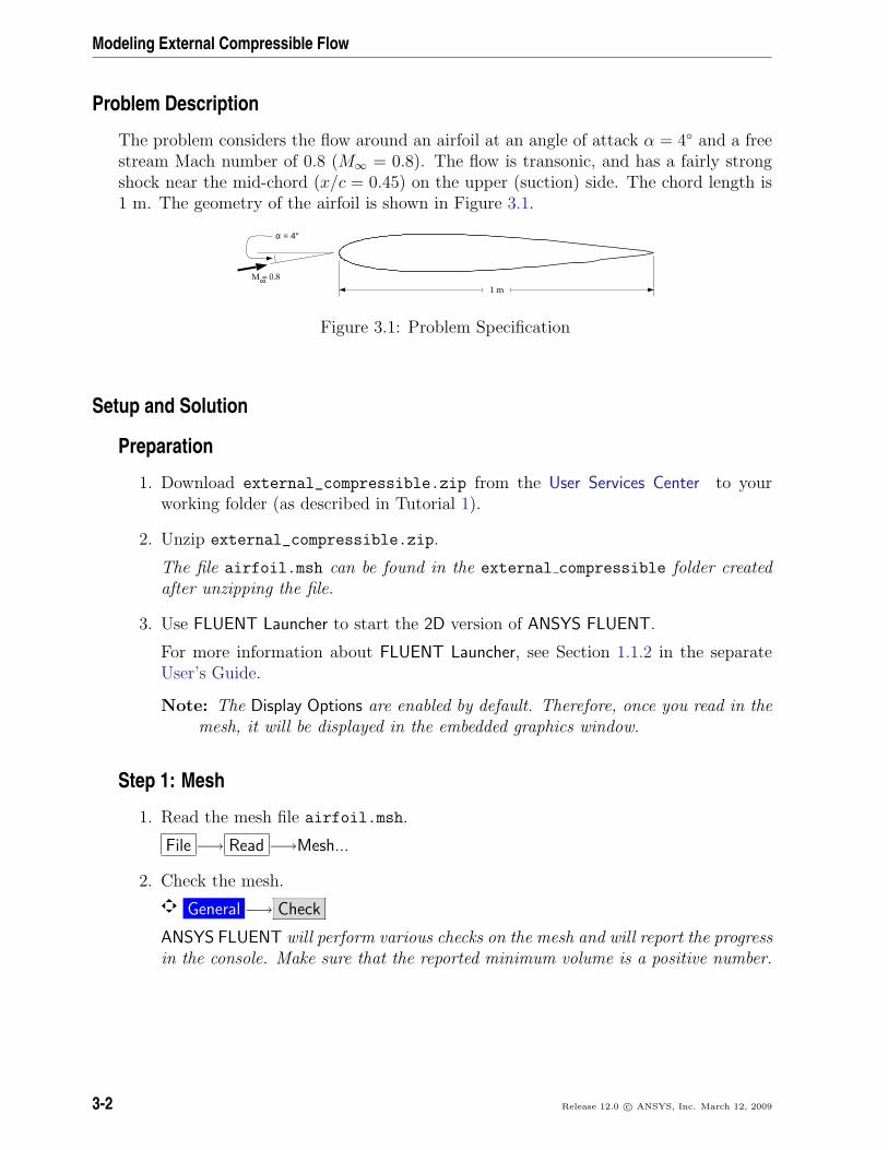
The problem considers the flow around an airfoil at an angle of attack α = 4◦ and a freestream Mach number of 0.8 (M∞ = 0.8). The flow is transonic, and has a fairly strongshock near the mid-chord (x/c = 0.45) on the upper (suction) side. The chord length is1 m. The geometry of the airfoil is shown in Figure 3.1.
M = 0.8∞
α = 4°
1 m
Figure 3.1: Problem Specification
Setup and Solution
Preparation
1. Download external_compressible.zip from the User Services Center to yourworking folder (as described in Tutorial 1).
2. Unzip external_compressible.zip.
The file airfoil.msh can be found in the external compressible folder createdafter unzipping the file.
3. Use FLUENT Launcher to start the 2D version of ANSYS FLUENT.
For more information about FLUENT Launcher, see Section 1.1.2 in the separateUser’s Guide.
Note: The Display Options are enabled by default. Therefore, once you read in themesh, it will be displayed in the embedded graphics window.
Step 1: Mesh
1. Read the mesh file airfoil.msh.
File −→ Read −→Mesh...
2. Check the mesh.
General −→ Check
ANSYS FLUENT will perform various checks on the mesh and will report the progressin the console. Make sure that the reported minimum volume is a positive number.
3-2 Release 12.0 c© ANSYS, Inc. March 12, 2009
Modeling External Compressible Flow
MeshFLUENT 12.0 (2d, pbns, lam)
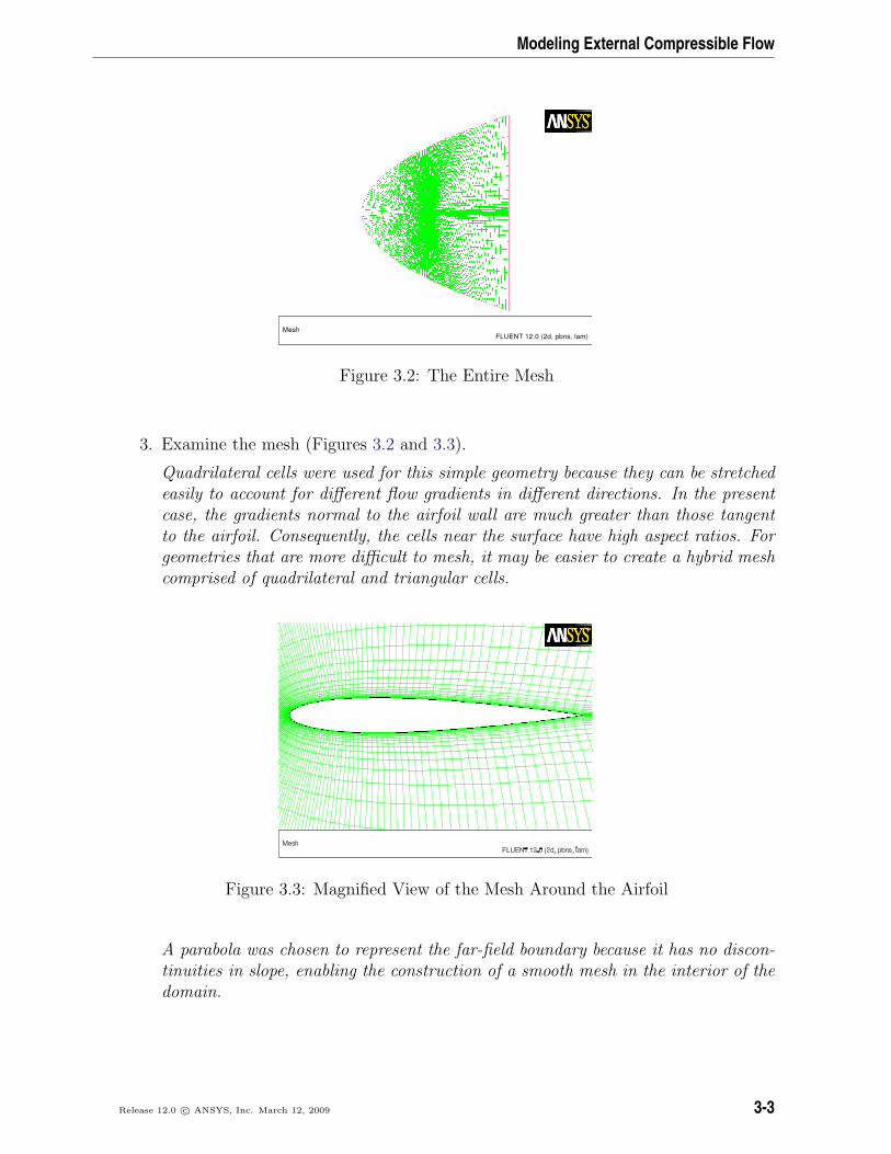
Figure 3.2: The Entire Mesh
3. Examine the mesh (Figures 3.2 and 3.3).
Quadrilateral cells were used for this simple geometry because they can be stretchedeasily to account for different flow gradients in different directions. In the presentcase, the gradients normal to the airfoil wall are much greater than those tangentto the airfoil. Consequently, the cells near the surface have high aspect ratios. Forgeometries that are more difficult to mesh, it may be easier to create a hybrid meshcomprised of quadrilateral and triangular cells.
Figure 3.3: Magnified View of the Mesh Around the Airfoil
A parabola was chosen to represent the far-field boundary because it has no discon-tinuities in slope, enabling the construction of a smooth mesh in the interior of thedomain.
Release 12.0 c© ANSYS, Inc. March 12, 2009 3-3
Modeling External Compressible Flow
Extra: You can use the right mouse button to probe for mesh information in thegraphics window. If you click the right mouse button on any node in themesh, information will be displayed in the ANSYS FLUENT console about theassociated zone, including the name of the zone. This feature is especiallyuseful when you have several zones of the same type and you want to distinguishbetween them quickly.
4. Reorder the mesh.
Mesh −→ Reorder −→Domain
This is done to reduce the bandwidth of the cell neighbor number and to speed upthe computations. This is especially important for large cases involving 1 million ormore cells. The method used to reorder the domain is the Reverse Cuthill-McKeemethod.
Step 2: General Settings
General
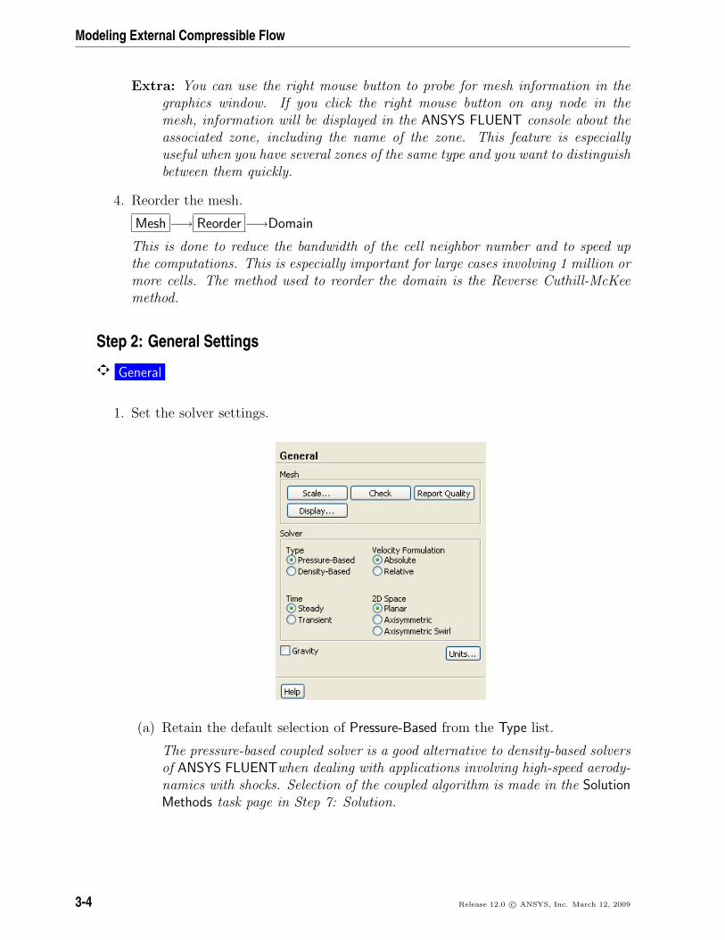
1. Set the solver settings.
(a) Retain the default selection of Pressure-Based from the Type list.
The pressure-based coupled solver is a good alternative to density-based solversof ANSYS FLUENTwhen dealing with applications involving high-speed aerody-namics with shocks. Selection of the coupled algorithm is made in the SolutionMethods task page in Step 7: Solution.
3-4 Release 12.0 c© ANSYS, Inc. March 12, 2009
Modeling External Compressible Flow
Step 3: Models
Models
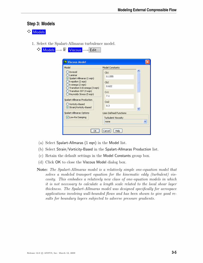
1. Select the Spalart-Allmaras turbulence model.
Models −→ Viscous −→ Edit...
(a) Select Spalart-Allmaras (1 eqn) in the Model list.
(b) Select Strain/Vorticity-Based in the Spalart-Allmaras Production list.
(c) Retain the default settings in the Model Constants group box.
(d) Click OK to close the Viscous Model dialog box.
Note: The Spalart-Allmaras model is a relatively simple one-equation model thatsolves a modeled transport equation for the kinematic eddy (turbulent) vis-cosity. This embodies a relatively new class of one-equation models in whichit is not necessary to calculate a length scale related to the local shear layerthickness. The Spalart-Allmaras model was designed specifically for aerospaceapplications involving wall-bounded flows and has been shown to give good re-sults for boundary layers subjected to adverse pressure gradients.
Release 12.0 c© ANSYS, Inc. March 12, 2009 3-5
Modeling External Compressible Flow
Step 4: Materials
Materials
The default Fluid Material is air, which is the working fluid in this problem. The defaultsettings need to be modified to account for compressibility and variations of the thermo-physical properties with temperature.
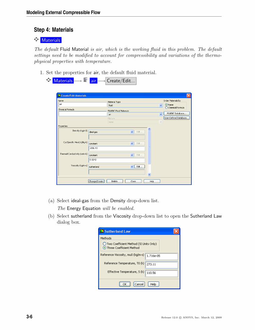
1. Set the properties for air, the default fluid material.
Materials −→ air −→ Create/Edit...
(a) Select ideal-gas from the Density drop-down list.
The Energy Equation will be enabled.
(b) Select sutherland from the Viscosity drop-down list to open the Sutherland Lawdialog box.
3-6 Release 12.0 c© ANSYS, Inc. March 12, 2009
Modeling External Compressible Flow
Scroll down the Viscosity drop-down list to find sutherland.
i. Retain the default selection of Three Coefficient Method in the Methodslist.
ii. Click OK to close the Sutherland Law dialog box.
The Sutherland law for viscosity is well suited for high-speed compressibleflows.
(c) Click Change/Create to save these settings.
(d) Close the Create/Edit Materials dialog box.
While Density and Viscosity have been made temperature dependent, Cp and ThermalConductivity have been left constant. For high-speed compressible flows, thermaldependency of the physical properties is generally recommended. For simplicity,Thermal Conductivity and Cp are assumed to be constant in this tutorial.
Step 5: Boundary Conditions
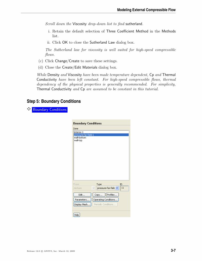
Boundary Conditions
Release 12.0 c© ANSYS, Inc. March 12, 2009 3-7
Modeling External Compressible Flow
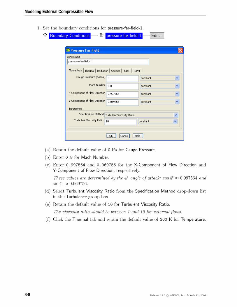
1. Set the boundary conditions for pressure-far-field-1.
Boundary Conditions −→ pressure-far-field-1 −→ Edit...
(a) Retain the default value of 0 Pa for Gauge Pressure.
(b) Enter 0.8 for Mach Number.
(c) Enter 0.997564 and 0.069756 for the X-Component of Flow Direction andY-Component of Flow Direction, respectively.
These values are determined by the 4◦ angle of attack: cos 4◦ ≈ 0.997564 andsin 4◦ ≈ 0.069756.
(d) Select Turbulent Viscosity Ratio from the Specification Method drop-down listin the Turbulence group box.
(e) Retain the default value of 10 for Turbulent Viscosity Ratio.
The viscosity ratio should be between 1 and 10 for external flows.
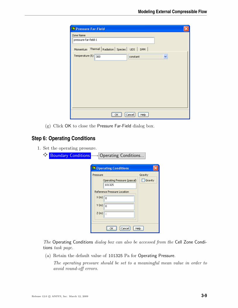
(f) Click the Thermal tab and retain the default value of 300 K for Temperature.
3-8 Release 12.0 c© ANSYS, Inc. March 12, 2009
Modeling External Compressible Flow
(g) Click OK to close the Pressure Far-Field dialog box.
Step 6: Operating Conditions
1. Set the operating pressure.
Boundary Conditions −→ Operating Conditions...
The Operating Conditions dialog box can also be accessed from the Cell Zone Condi-tions task page.
(a) Retain the default value of 101325 Pa for Operating Pressure.
The operating pressure should be set to a meaningful mean value in order toavoid round-off errors.
Release 12.0 c© ANSYS, Inc. March 12, 2009 3-9
Modeling External Compressible Flow
(b) Click OK to close the Operating Conditions dialog box.
For information about setting the operating pressure, see Section 8.14 in the separateUser’s Guide.
Step 7: Solution
Solution
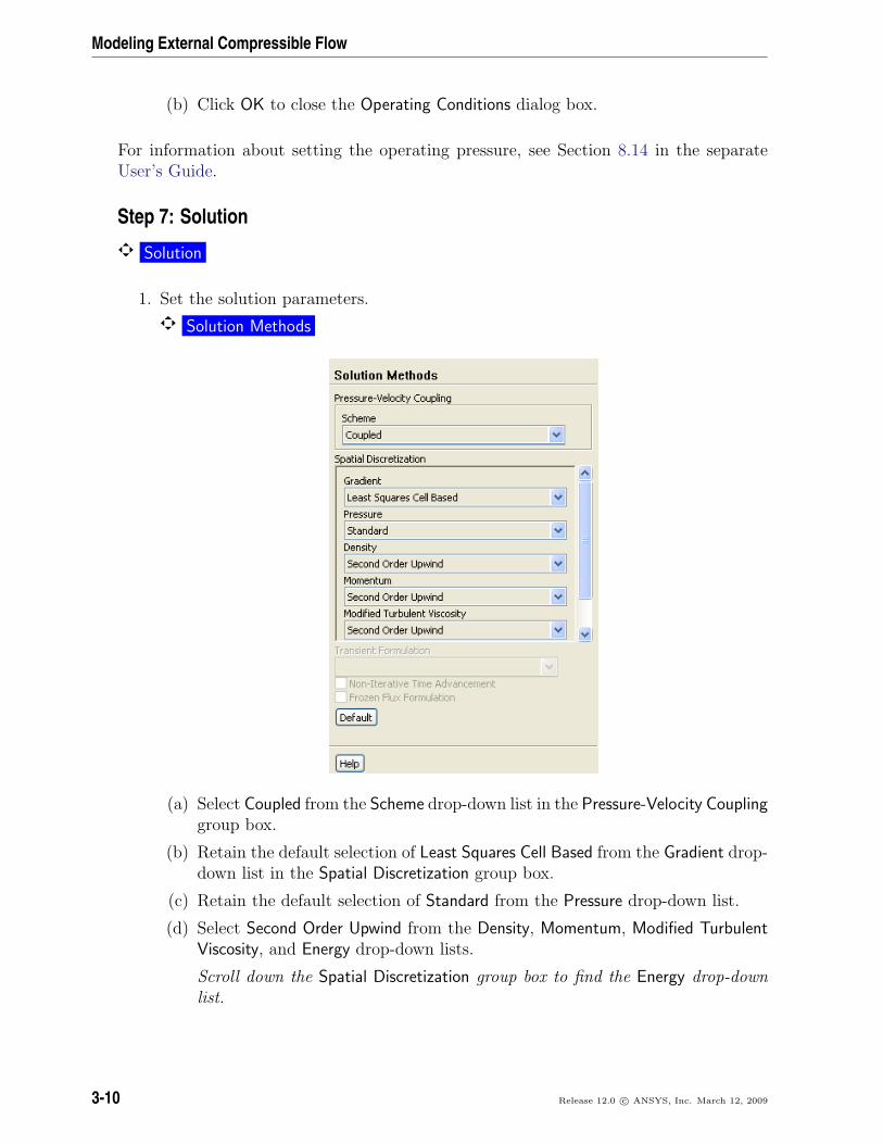
1. Set the solution parameters.
Solution Methods
(a) Select Coupled from the Scheme drop-down list in the Pressure-Velocity Couplinggroup box.
(b) Retain the default selection of Least Squares Cell Based from the Gradient drop-down list in the Spatial Discretization group box.
(c) Retain the default selection of Standard from the Pressure drop-down list.
(d) Select Second Order Upwind from the Density, Momentum, Modified TurbulentViscosity, and Energy drop-down lists.
Scroll down the Spatial Discretization group box to find the Energy drop-downlist.
3-10 Release 12.0 c© ANSYS, Inc. March 12, 2009
Modeling External Compressible Flow
The second-order scheme will resolve the boundary layer and shock more ac-curately than the first-order scheme.
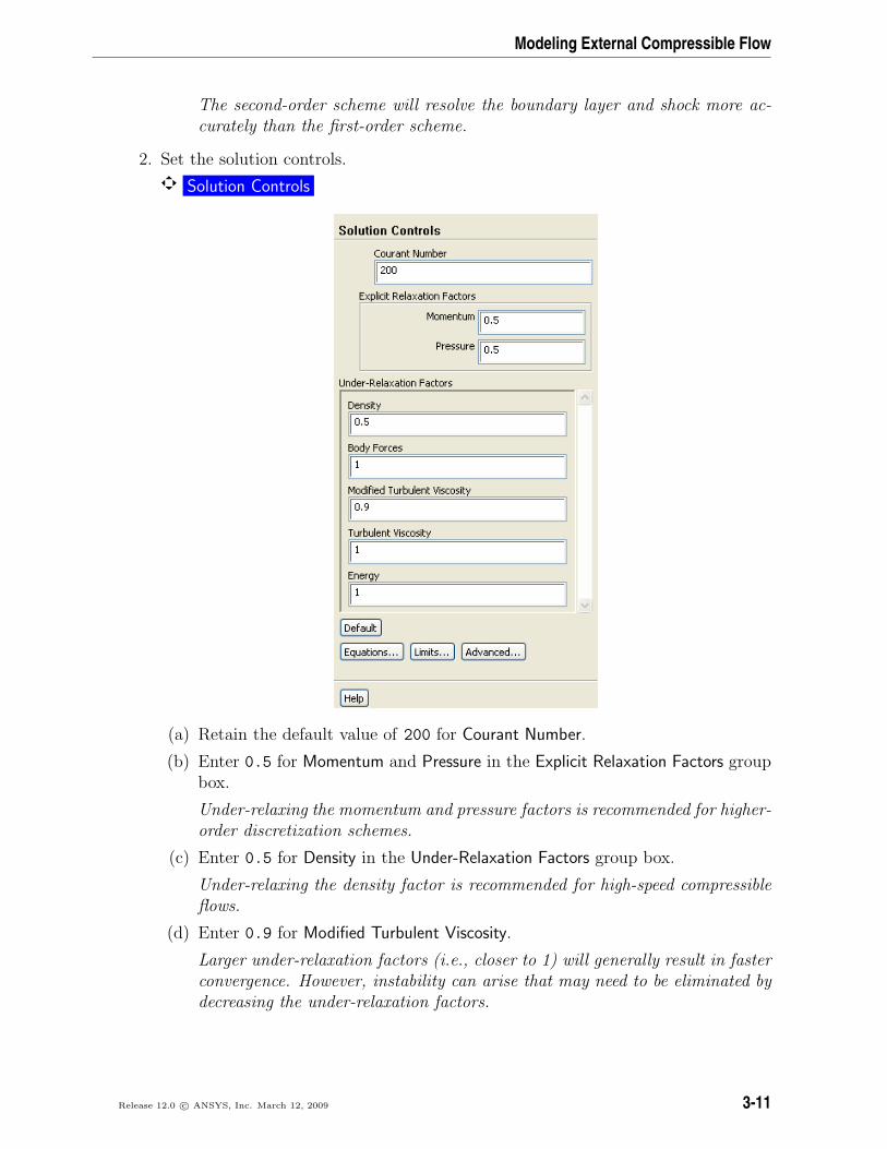
2. Set the solution controls.
Solution Controls
(a) Retain the default value of 200 for Courant Number.
(b) Enter 0.5 for Momentum and Pressure in the Explicit Relaxation Factors groupbox.
Under-relaxing the momentum and pressure factors is recommended for higher-order discretization schemes.
(c) Enter 0.5 for Density in the Under-Relaxation Factors group box.
Under-relaxing the density factor is recommended for high-speed compressibleflows.
(d) Enter 0.9 for Modified Turbulent Viscosity.
Larger under-relaxation factors (i.e., closer to 1) will generally result in fasterconvergence. However, instability can arise that may need to be eliminated bydecreasing the under-relaxation factors.
Release 12.0 c© ANSYS, Inc. March 12, 2009 3-11
Modeling External Compressible Flow
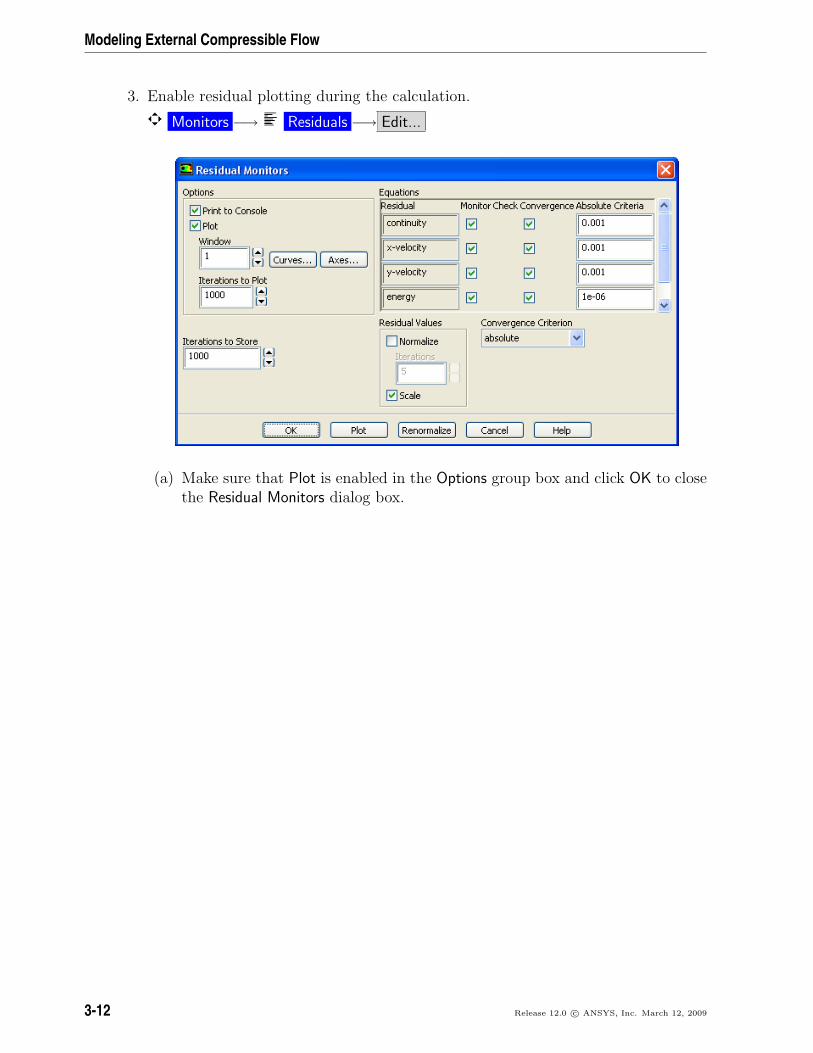
3. Enable residual plotting during the calculation.
Monitors −→ Residuals −→ Edit...
(a) Make sure that Plot is enabled in the Options group box and click OK to closethe Residual Monitors dialog box.
3-12 Release 12.0 c© ANSYS, Inc. March 12, 2009
Modeling External Compressible Flow
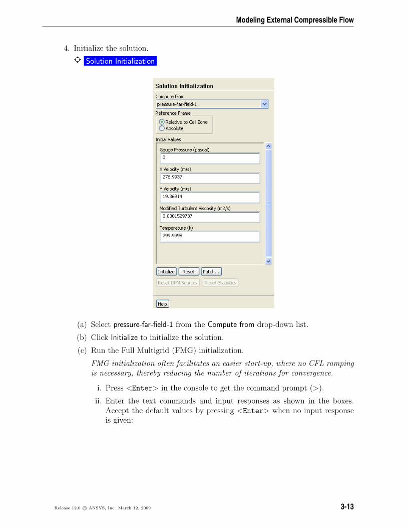
4. Initialize the solution.
Solution Initialization
(a) Select pressure-far-field-1 from the Compute from drop-down list.
(b) Click Initialize to initialize the solution.
(c) Run the Full Multigrid (FMG) initialization.
FMG initialization often facilitates an easier start-up, where no CFL rampingis necessary, thereby reducing the number of iterations for convergence.
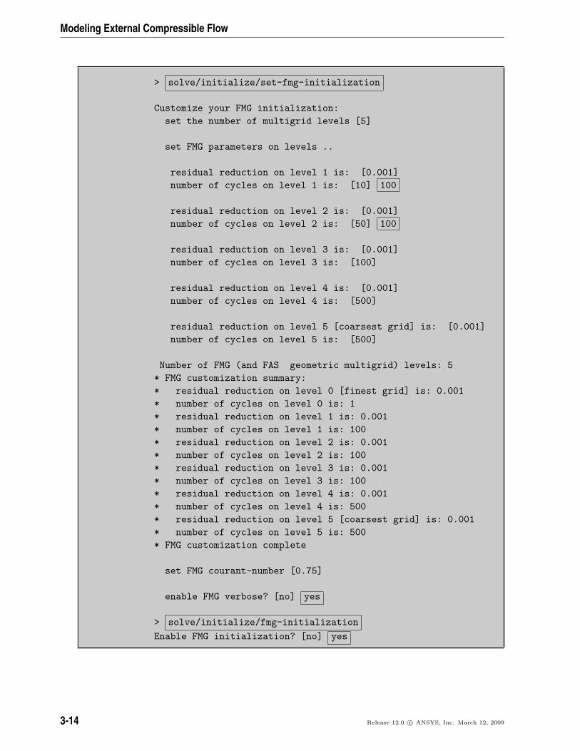
i. Press <Enter> in the console to get the command prompt (>).
ii. Enter the text commands and input responses as shown in the boxes.Accept the default values by pressing <Enter> when no input responseis given:
Release 12.0 c© ANSYS, Inc. March 12, 2009 3-13
Modeling External Compressible Flow
> solve/initialize/set-fmg-initialization
Customize your FMG initialization:set the number of multigrid levels [5]
set FMG parameters on levels ..
residual reduction on level 1 is: [0.001]number of cycles on level 1 is: [10] 100
residual reduction on level 2 is: [0.001]number of cycles on level 2 is: [50] 100
residual reduction on level 3 is: [0.001]number of cycles on level 3 is: [100]
residual reduction on level 4 is: [0.001]number of cycles on level 4 is: [500]
residual reduction on level 5 [coarsest grid] is: [0.001]number of cycles on level 5 is: [500]
Number of FMG (and FAS geometric multigrid) levels: 5* FMG customization summary:* residual reduction on level 0 [finest grid] is: 0.001* number of cycles on level 0 is: 1* residual reduction on level 1 is: 0.001* number of cycles on level 1 is: 100* residual reduction on level 2 is: 0.001* number of cycles on level 2 is: 100* residual reduction on level 3 is: 0.001* number of cycles on level 3 is: 100* residual reduction on level 4 is: 0.001* number of cycles on level 4 is: 500* residual reduction on level 5 [coarsest grid] is: 0.001* number of cycles on level 5 is: 500* FMG customization complete
set FMG courant-number [0.75]
enable FMG verbose? [no] yes
> solve/initialize/fmg-initialization
Enable FMG initialization? [no] yes
3-14 Release 12.0 c© ANSYS, Inc. March 12, 2009
Modeling External Compressible Flow
Note: Whenever FMG initialization is performed, it is important to inspect theFMG initialized flow field using postprocessing tools of ANSYS FLUENT. Mon-itoring the normalized residuals, which are plotted in the console window willgive you an idea of the convergence of the FMG solver. You should noticethat the value of the normalized residuals decreases. For information aboutFMG initialization, including convergence strategies, see Section 26.10 in theseparate User’s Guide.
5. Save the case and data files (airfoil.cas and airfoil.dat).
File −→ Write −→Case & Data...
It is good practice to save the case and data files during several stages of your casesetup.
6. Start the calculation by requesting 50 iterations.
Run Calculation
(a) Enter 50 for Number of Iterations.
(b) Click Calculate.
By performing some iterations before setting up the force monitors, you will avoidlarge initial transients in the monitor plots. This will reduce the axes range andmake it easier to judge the convergence.
Release 12.0 c© ANSYS, Inc. March 12, 2009 3-15
Modeling External Compressible Flow
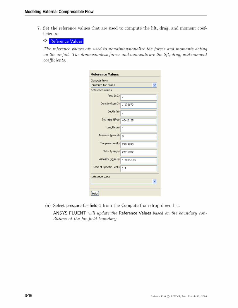
7. Set the reference values that are used to compute the lift, drag, and moment coef-ficients.
Reference Values
The reference values are used to nondimensionalize the forces and moments actingon the airfoil. The dimensionless forces and moments are the lift, drag, and momentcoefficients.
(a) Select pressure-far-field-1 from the Compute from drop-down list.
ANSYS FLUENT will update the Reference Values based on the boundary con-ditions at the far-field boundary.
3-16 Release 12.0 c© ANSYS, Inc. March 12, 2009
Modeling External Compressible Flow
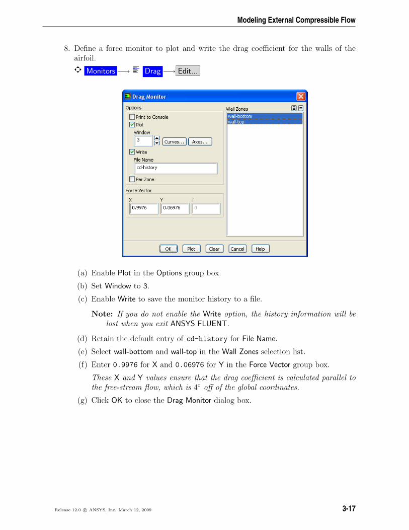
8. Define a force monitor to plot and write the drag coefficient for the walls of theairfoil.
Monitors −→ Drag −→ Edit...
(a) Enable Plot in the Options group box.
(b) Set Window to 3.
(c) Enable Write to save the monitor history to a file.
Note: If you do not enable the Write option, the history information will belost when you exit ANSYS FLUENT.
(d) Retain the default entry of cd-history for File Name.
(e) Select wall-bottom and wall-top in the Wall Zones selection list.
(f) Enter 0.9976 for X and 0.06976 for Y in the Force Vector group box.
These X and Y values ensure that the drag coefficient is calculated parallel tothe free-stream flow, which is 4◦ off of the global coordinates.
(g) Click OK to close the Drag Monitor dialog box.
Release 12.0 c© ANSYS, Inc. March 12, 2009 3-17
Modeling External Compressible Flow
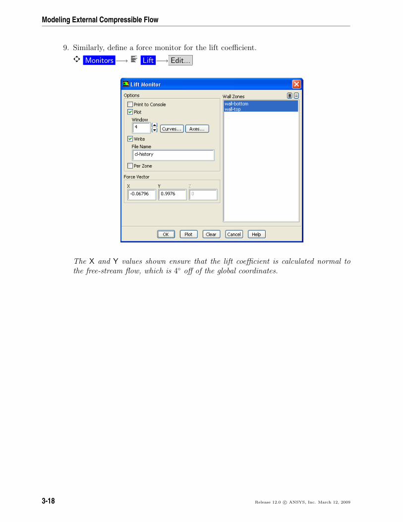
9. Similarly, define a force monitor for the lift coefficient.
Monitors −→ Lift −→ Edit...
The X and Y values shown ensure that the lift coefficient is calculated normal tothe free-stream flow, which is 4◦ off of the global coordinates.
3-18 Release 12.0 c© ANSYS, Inc. March 12, 2009
Modeling External Compressible Flow
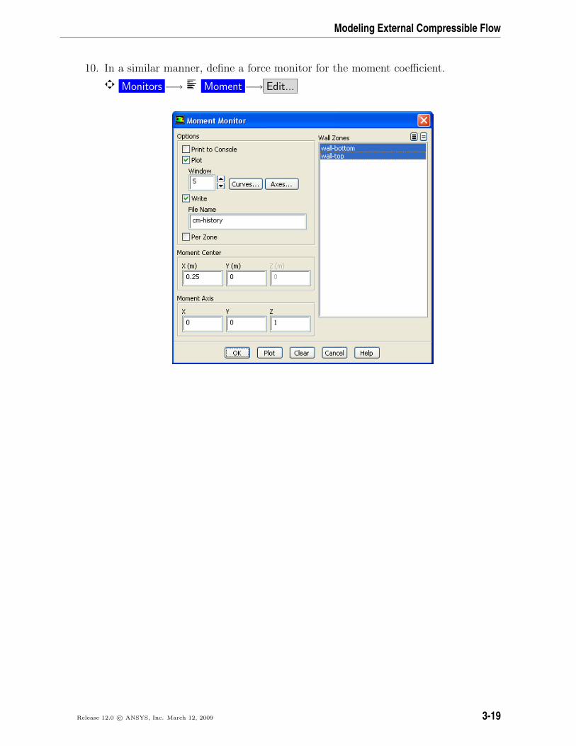
10. In a similar manner, define a force monitor for the moment coefficient.
Monitors −→ Moment −→ Edit...
Release 12.0 c© ANSYS, Inc. March 12, 2009 3-19
Modeling External Compressible Flow
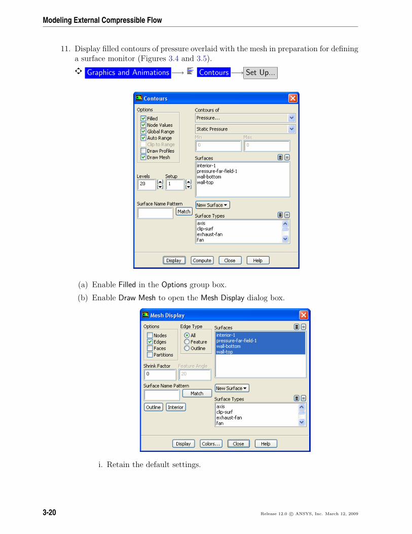
11. Display filled contours of pressure overlaid with the mesh in preparation for defininga surface monitor (Figures 3.4 and 3.5).
Graphics and Animations −→ Contours −→ Set Up...
(a) Enable Filled in the Options group box.
(b) Enable Draw Mesh to open the Mesh Display dialog box.
i. Retain the default settings.
3-20 Release 12.0 c© ANSYS, Inc. March 12, 2009
Modeling External Compressible Flow
ii. Close the Mesh Display dialog box.
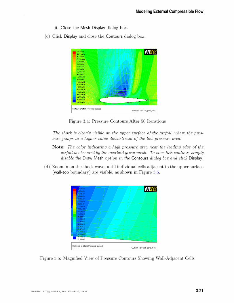
(c) Click Display and close the Contours dialog box.
Figure 3.4: Pressure Contours After 50 Iterations
The shock is clearly visible on the upper surface of the airfoil, where the pres-sure jumps to a higher value downstream of the low pressure area.
Note: The color indicating a high pressure area near the leading edge of theairfoil is obscured by the overlaid green mesh. To view this contour, simplydisable the Draw Mesh option in the Contours dialog box and click Display.
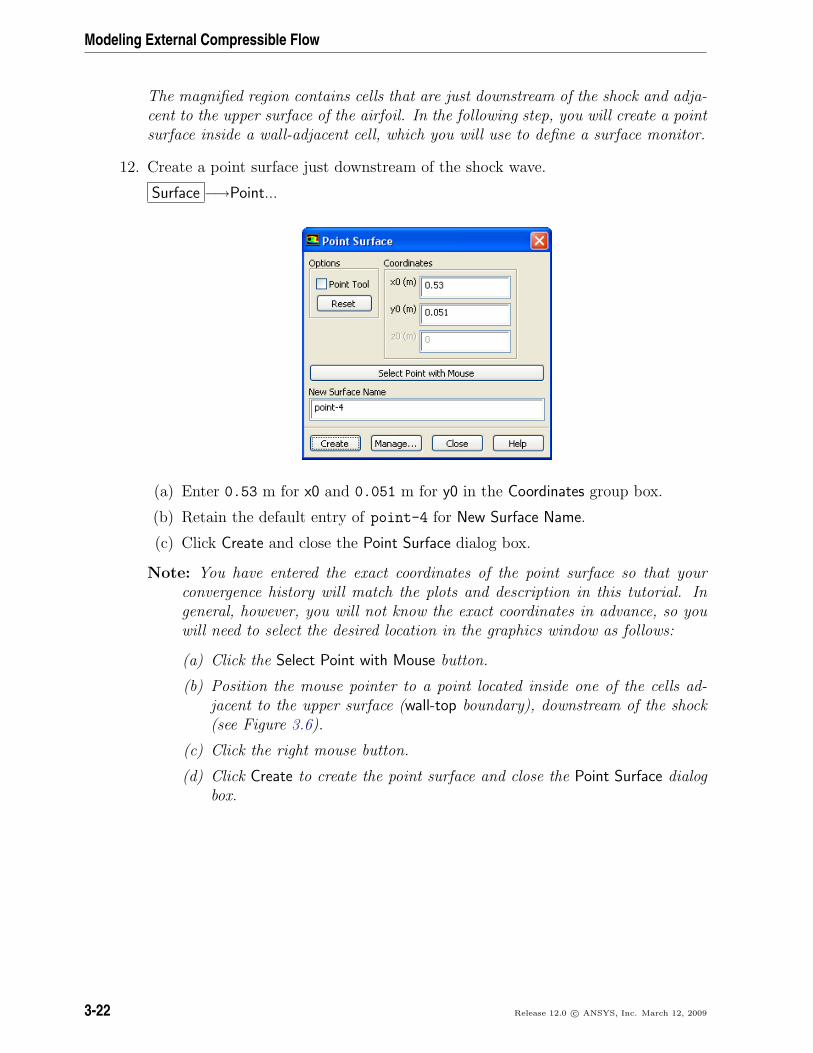
(d) Zoom in on the shock wave, until individual cells adjacent to the upper surface(wall-top boundary) are visible, as shown in Figure 3.5.
Contours of Static Pressure (pascal)FLUENT 12.0 (2d, pbns, S-A)
5.43e+044.87e+044.31e+043.76e+043.20e+042.65e+042.09e+041.53e+049.79e+034.23e+03-1.33e+0-6.89e+0-1.25e+0-1.80e+0-2.36e+0-2.91e+0-3.47e+0-4.03e+0-4.58e+0-5.14e+0-5.69e+0
Figure 3.5: Magnified View of Pressure Contours Showing Wall-Adjacent Cells
Release 12.0 c© ANSYS, Inc. March 12, 2009 3-21
Modeling External Compressible Flow
The magnified region contains cells that are just downstream of the shock and adja-cent to the upper surface of the airfoil. In the following step, you will create a pointsurface inside a wall-adjacent cell, which you will use to define a surface monitor.
12. Create a point surface just downstream of the shock wave.
Surface −→Point...
(a) Enter 0.53 m for x0 and 0.051 m for y0 in the Coordinates group box.
(b) Retain the default entry of point-4 for New Surface Name.
(c) Click Create and close the Point Surface dialog box.
Note: You have entered the exact coordinates of the point surface so that yourconvergence history will match the plots and description in this tutorial. Ingeneral, however, you will not know the exact coordinates in advance, so youwill need to select the desired location in the graphics window as follows:
(a) Click the Select Point with Mouse button.
(b) Position the mouse pointer to a point located inside one of the cells ad-jacent to the upper surface (wall-top boundary), downstream of the shock(see Figure 3.6).
(c) Click the right mouse button.
(d) Click Create to create the point surface and close the Point Surface dialogbox.
3-22 Release 12.0 c© ANSYS, Inc. March 12, 2009
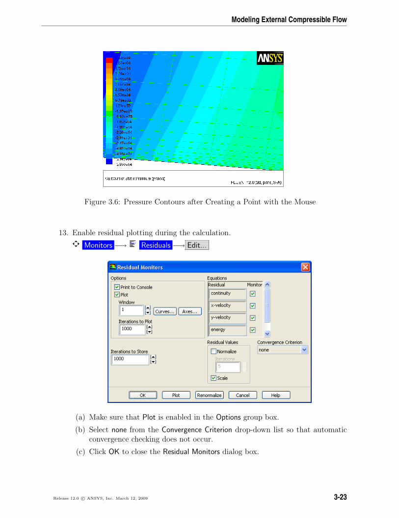
Modeling External Compressible Flow
Figure 3.6: Pressure Contours after Creating a Point with the Mouse
13. Enable residual plotting during the calculation.
Monitors −→ Residuals −→ Edit...
(a) Make sure that Plot is enabled in the Options group box.
(b) Select none from the Convergence Criterion drop-down list so that automaticconvergence checking does not occur.
(c) Click OK to close the Residual Monitors dialog box.
Release 12.0 c© ANSYS, Inc. March 12, 2009 3-23
Modeling External Compressible Flow
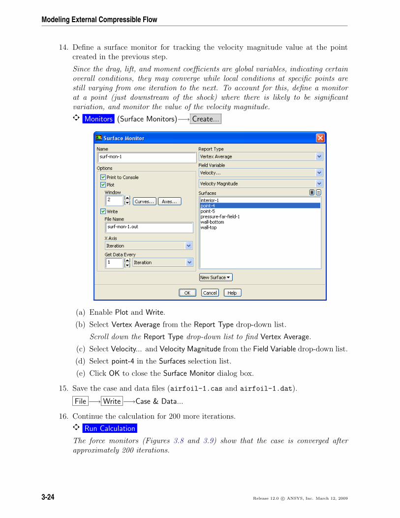
14. Define a surface monitor for tracking the velocity magnitude value at the pointcreated in the previous step.
Since the drag, lift, and moment coefficients are global variables, indicating certainoverall conditions, they may converge while local conditions at specific points arestill varying from one iteration to the next. To account for this, define a monitorat a point (just downstream of the shock) where there is likely to be significantvariation, and monitor the value of the velocity magnitude.
Monitors (Surface Monitors)−→ Create...
(a) Enable Plot and Write.
(b) Select Vertex Average from the Report Type drop-down list.
Scroll down the Report Type drop-down list to find Vertex Average.
(c) Select Velocity... and Velocity Magnitude from the Field Variable drop-down list.
(d) Select point-4 in the Surfaces selection list.
(e) Click OK to close the Surface Monitor dialog box.
15. Save the case and data files (airfoil-1.cas and airfoil-1.dat).
File −→ Write −→Case & Data...
16. Continue the calculation for 200 more iterations.
Run Calculation
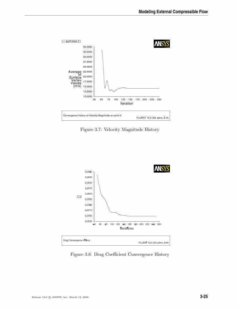
The force monitors (Figures 3.8 and 3.9) show that the case is converged afterapproximately 200 iterations.
3-24 Release 12.0 c© ANSYS, Inc. March 12, 2009
Modeling External Compressible Flow
Convergence history of Velocity Magnitude on point-4FLUENT 12.0 (2d, pbns, S-A)
Iteration
(m/s)ValuesVertex
Surfaceof
Average
250225200175150125100755025
35.0000
32.5000
30.0000
27.5000
25.0000
22.5000
20.0000
17.5000
15.0000
12.5000
10.0000
surf-mon-1
Figure 3.7: Velocity Magnitude History
Figure 3.8: Drag Coefficient Convergence History
Release 12.0 c© ANSYS, Inc. March 12, 2009 3-25

Modeling External Compressible Flow
Figure 3.9: Lift Coefficient Convergence History
Figure 3.10: Moment Coefficient Convergence History
17. Save the case and data files (airfoil-2.cas and airfoil-2.dat).
File −→ Write −→Case & Data...
3-26 Release 12.0 c© ANSYS, Inc. March 12, 2009
Modeling External Compressible Flow
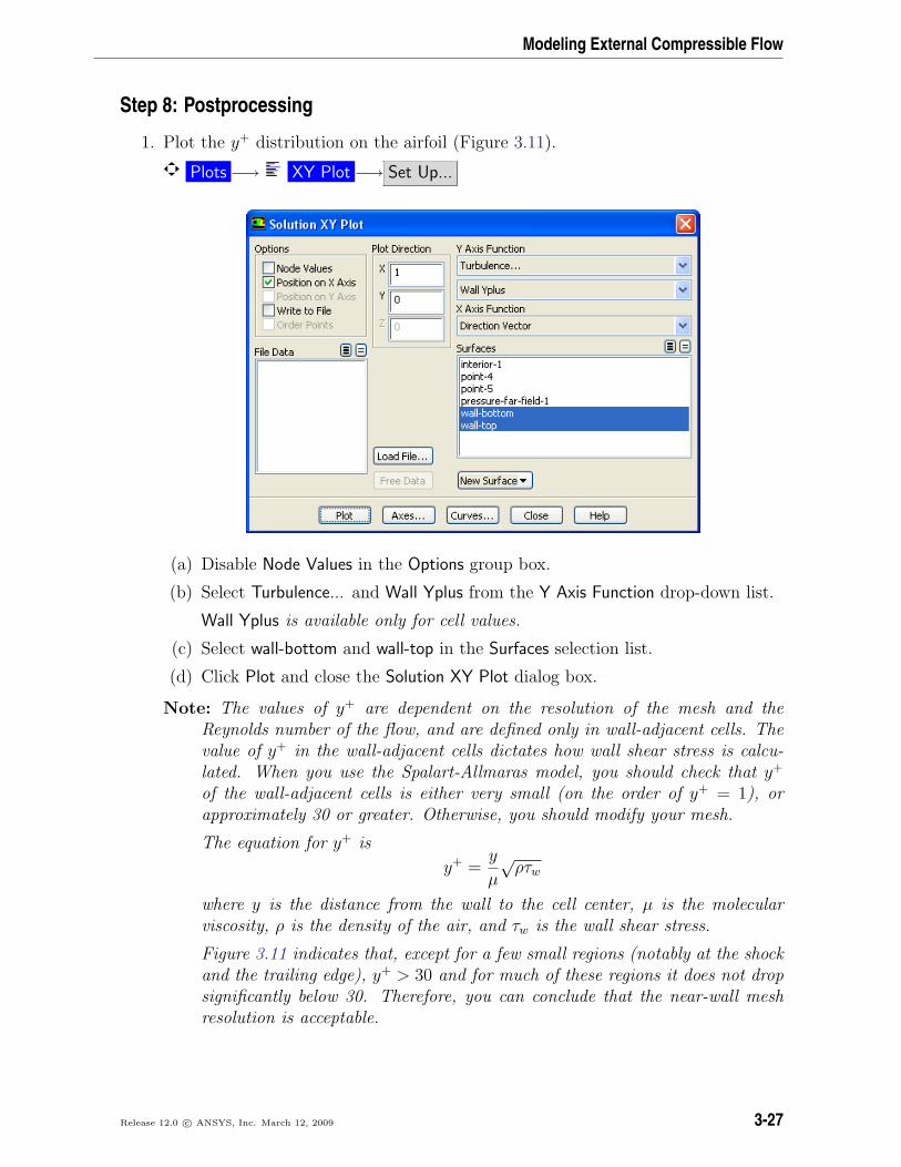
Step 8: Postprocessing
1. Plot the y+ distribution on the airfoil (Figure 3.11).
Plots −→ XY Plot −→ Set Up...
(a) Disable Node Values in the Options group box.
(b) Select Turbulence... and Wall Yplus from the Y Axis Function drop-down list.
Wall Yplus is available only for cell values.
(c) Select wall-bottom and wall-top in the Surfaces selection list.
(d) Click Plot and close the Solution XY Plot dialog box.
Note: The values of y+ are dependent on the resolution of the mesh and theReynolds number of the flow, and are defined only in wall-adjacent cells. Thevalue of y+ in the wall-adjacent cells dictates how wall shear stress is calcu-lated. When you use the Spalart-Allmaras model, you should check that y+
of the wall-adjacent cells is either very small (on the order of y+ = 1), orapproximately 30 or greater. Otherwise, you should modify your mesh.
The equation for y+ is
y+ =y
µ
√ρτw
where y is the distance from the wall to the cell center, µ is the molecularviscosity, ρ is the density of the air, and τw is the wall shear stress.
Figure 3.11 indicates that, except for a few small regions (notably at the shockand the trailing edge), y+ > 30 and for much of these regions it does not dropsignificantly below 30. Therefore, you can conclude that the near-wall meshresolution is acceptable.
Release 12.0 c© ANSYS, Inc. March 12, 2009 3-27
Modeling External Compressible Flow
Figure 3.11: XY Plot of y+ Distribution
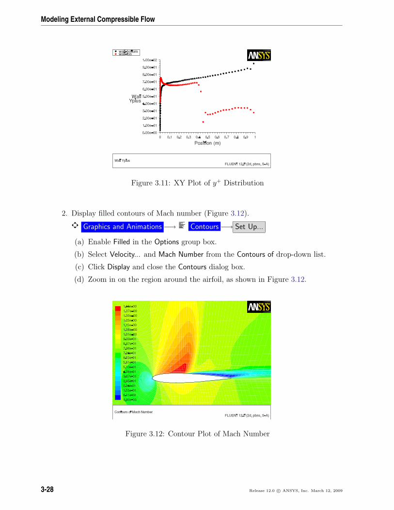
2. Display filled contours of Mach number (Figure 3.12).
Graphics and Animations −→ Contours −→ Set Up...
(a) Enable Filled in the Options group box.
(b) Select Velocity... and Mach Number from the Contours of drop-down list.
(c) Click Display and close the Contours dialog box.
(d) Zoom in on the region around the airfoil, as shown in Figure 3.12.
Figure 3.12: Contour Plot of Mach Number
3-28 Release 12.0 c© ANSYS, Inc. March 12, 2009
Modeling External Compressible Flow
Note the discontinuity, in this case a shock, on the upper surface of the airfoilin Figure 3.12 at about x/c ≈ 0.45.
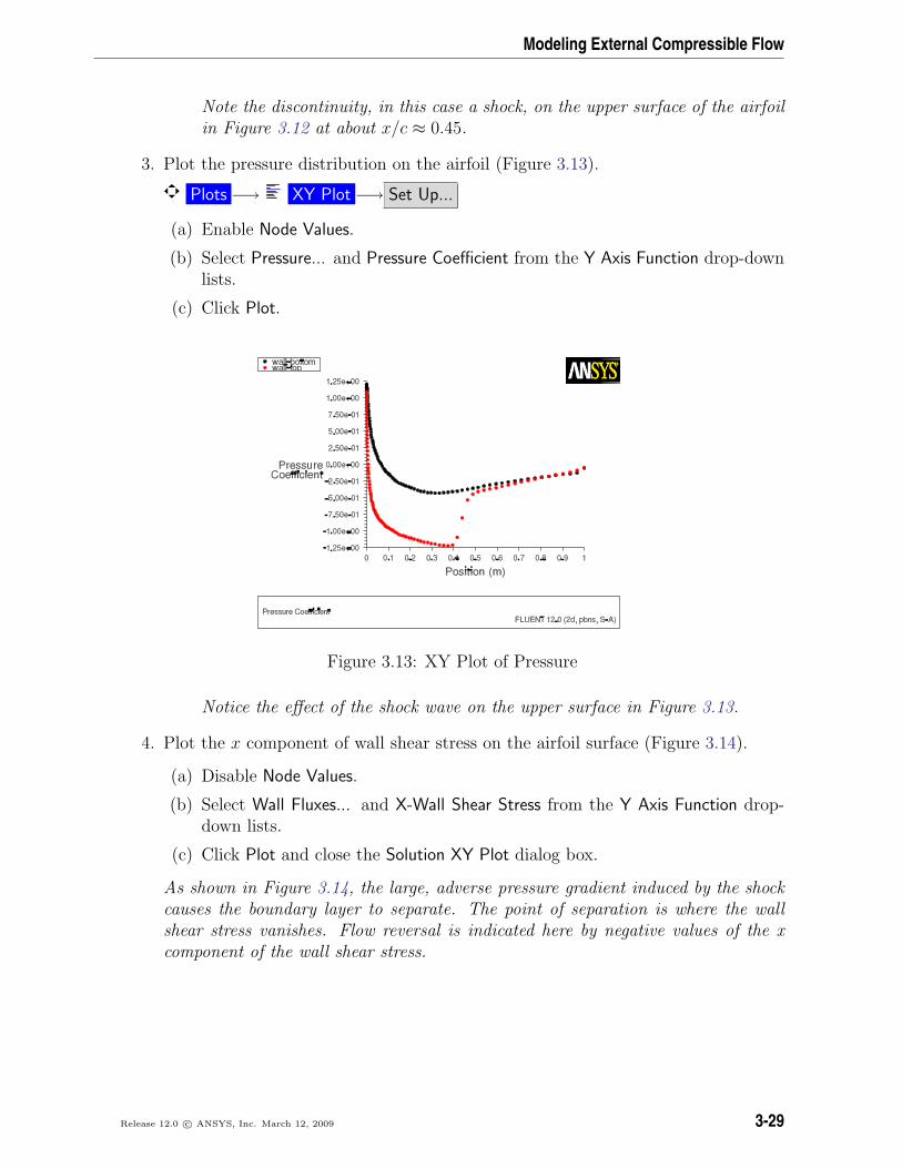
3. Plot the pressure distribution on the airfoil (Figure 3.13).
Plots −→ XY Plot −→ Set Up...
(a) Enable Node Values.
(b) Select Pressure... and Pressure Coefficient from the Y Axis Function drop-downlists.
(c) Click Plot.
Figure 3.13: XY Plot of Pressure
Notice the effect of the shock wave on the upper surface in Figure 3.13.
4. Plot the x component of wall shear stress on the airfoil surface (Figure 3.14).
(a) Disable Node Values.
(b) Select Wall Fluxes... and X-Wall Shear Stress from the Y Axis Function drop-down lists.
(c) Click Plot and close the Solution XY Plot dialog box.
As shown in Figure 3.14, the large, adverse pressure gradient induced by the shockcauses the boundary layer to separate. The point of separation is where the wallshear stress vanishes. Flow reversal is indicated here by negative values of the xcomponent of the wall shear stress.
Release 12.0 c© ANSYS, Inc. March 12, 2009 3-29
Modeling External Compressible Flow
Figure 3.14: XY Plot of x Wall Shear Stress
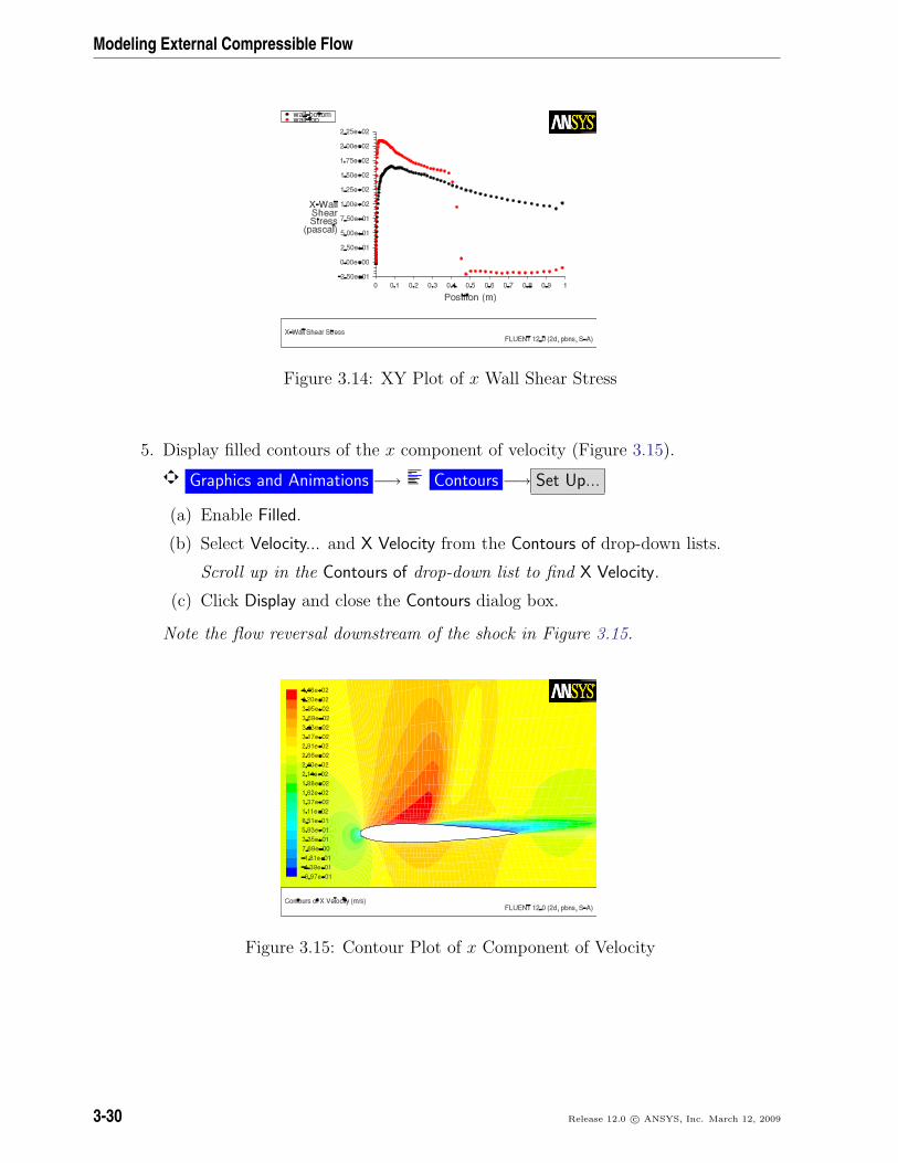
5. Display filled contours of the x component of velocity (Figure 3.15).
Graphics and Animations −→ Contours −→ Set Up...
(a) Enable Filled.
(b) Select Velocity... and X Velocity from the Contours of drop-down lists.
Scroll up in the Contours of drop-down list to find X Velocity.
(c) Click Display and close the Contours dialog box.
Note the flow reversal downstream of the shock in Figure 3.15.
Figure 3.15: Contour Plot of x Component of Velocity
3-30 Release 12.0 c© ANSYS, Inc. March 12, 2009
Modeling External Compressible Flow
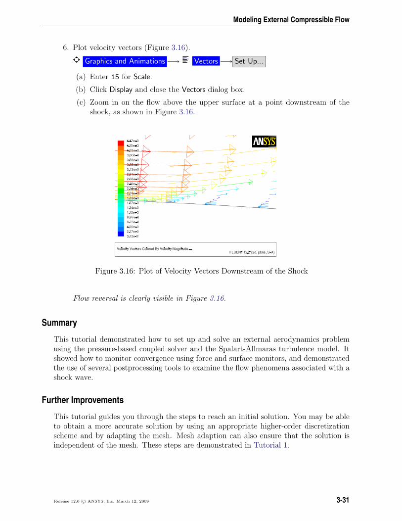
6. Plot velocity vectors (Figure 3.16).
Graphics and Animations −→ Vectors −→ Set Up...
(a) Enter 15 for Scale.
(b) Click Display and close the Vectors dialog box.
(c) Zoom in on the flow above the upper surface at a point downstream of theshock, as shown in Figure 3.16.
Figure 3.16: Plot of Velocity Vectors Downstream of the Shock
Flow reversal is clearly visible in Figure 3.16.
Summary
This tutorial demonstrated how to set up and solve an external aerodynamics problemusing the pressure-based coupled solver and the Spalart-Allmaras turbulence model. Itshowed how to monitor convergence using force and surface monitors, and demonstratedthe use of several postprocessing tools to examine the flow phenomena associated with ashock wave.
Further Improvements
This tutorial guides you through the steps to reach an initial solution. You may be ableto obtain a more accurate solution by using an appropriate higher-order discretizationscheme and by adapting the mesh. Mesh adaption can also ensure that the solution isindependent of the mesh. These steps are demonstrated in Tutorial 1.
Release 12.0 c© ANSYS, Inc. March 12, 2009 3-31

Modeling External Compressible Flow
3-32 Release 12.0 c© ANSYS, Inc. March 12, 2009