an efficient finite-volume scheme for modeling water ... · "an efficient finite-volume scheme...
TRANSCRIPT
Leon, A., M.S. Ghidaoui, A.R. Schmidt and M.H. Garcia. 2007. "An Efficient Finite-Volume Scheme for Modeling Water Hammer Flows." Journal of Water Management Modeling R227-21. doi: 10.14796/JWMM.R227-21.© CHI 2007 www.chijournal.org ISSN: 2292-6062 (Formerly in Contemporary Modeling of Urban Water Systems. ISBN: 0-9736716-3-7)
411
21 An Efficient Finite-Volume Scheme for
Modeling Water Hammer Flows Arturo S. León, Mohamed S. Ghidaoui, Arthur R. Schmidt and Marcelo H. García
The study of water hammer flows has great significance in a wide range of industrial and municipal applications including power plants, petroleum industries, water distribution systems, etc. The understanding of water hammer phenomena is also important in hydraulic conveyance systems such as stormwater and sanitary sewer systems. Although the latter two systems are generally designed based on gravity flow, in practice large variations in the inflow and outflow from these systems may result in the pressurization of the systems that, in turn, may produce water hammer phenomena. For modeling this type of flows, several numerical approaches have been proposed. The efficiency of a model is a critical factor for Real-Time Control (RTC), since several simulations are required within a control loop in order to optimize the control strategy, and small simulation time steps are needed to reproduce the rapidly varying hydraulics (León et al. 2006). RTC is becoming increasingly indispensable for industrial and municipal applications in general. For instance, in the case of water distribution systems, RTC facilitates delivery of safe, clean and high-quality water in the most expedient and economical manner.
Among the approaches proposed to solve the water hammer equations are the Method of Characteristics (MOC), Finite Differences (FD), Wave Characteristic Method (WCM), Finite Elements (FE), and Finite Volume (FV). In-depth discussions of these methods can be found in Chaudhry and

412 Finite-Volume Scheme for Modeling Water Hammer Flows
Hussaini 1985, Ghidaoui and Karney 1994, Szymkiewicz and Mitosek 2004, Zhao and Ghidaoui 2004, and Wood et al. 2005. Among these methods, MOC-based schemes are most popular because these schemes provide the desirable attributes of accuracy, numerical efficiency, programming simplicity, and ability to handle complex boundary conditions (e.g., Wylie and Streeter 1993; Ghidaoui et al. 2005; Zhao and Ghidaoui 2004). In fact, in a review of commercially available water hammer software packages, it is found that eleven out of fourteen software packages examined use MOC schemes (Ghidaoui et al. 2005).
Recently, FV Godunov-Type Schemes (GTS), which belong to the family of shock-capturing schemes, have been applied to water hammer problems with good success. The underlying idea of GTS is the Riemann problem that must be solved to provide fluxes between adjacent computational cells. The first application of GTS to water hammer problems is due to Guinot (2000), who presented first and second-order schemes based on Taylor series expansions of the Riemann invariants. He showed that his second-order scheme is largely superior to his first-order scheme, although the Taylor series development introduces an inevitable inaccuracy in the estimated pressure, especially in the case of low pressure-wave celerities. A second application is due to Hwang and Chung (2002), whose second-order accuracy scheme is based on the conservative form of the compressible flow equations. Although this scheme requires an iterative process to solve the Riemann problem, these authors state that their scheme requires a little more arithmetic operation and CPU time than the so-called Roe's scheme, but is able to get more accurate computational results than the latter scheme. Later, Zhao and Ghidaoui (2004) presented first and second-order schemes for solution of the non-conservative water hammer equations. They show that, for a given level of accuracy, their second-order GTS requires much less memory storage and execution time than either their first-order GTS or the fixed-grid MOC scheme with space-line interpolation. Although highly efficient, this chapter shows that the second-order scheme of Zhao and Ghidaoui (2004) has an overall accuracy of at most first-order.
The reason why the second-order scheme of Zhao and Ghidaoui (2004) has at most only first-order rate of convergence is because this scheme uses a second-order formulation solely at the internal cells, but not at the boundaries for which only a first-order formulation is used. This chapter focuses on the formulation and assessment of a second-order accurate (internal and boundary nodes) FV scheme for modeling water hammer flows. Unlike the scheme of Zhao and Ghidaoui (2004), the proposed approach uses the conservative form of the water hammer equations. To
Finite-Volume Scheme for Modeling Water Hammer Flows 413
achieve second-order accuracy at the internal cells in the proposed approach, the Monotone Upstream-centred Scheme for Conservation Laws (MUSCL) - Hancock method is used, which also was used by Zhao and Ghidaoui (2004). Thus, the only difference between the second-order scheme of Zhao and Ghidaoui and the proposed approach is in the order of accuracy used at the boundaries (first-order in the scheme of Zhao and Ghidaoui and second order in the proposed approach).
21.1 Governing Equations
The governing equations for water hammer flows are classically derived from the conservation of mass and momentum. For a pipe of constant diameter, the water hammer equations can be written in their vector conservative form as follows (e.g., Guinot 2003):
(21.1)
where the vector variable U, the flux vector F and the source term vector S may be written as:
(21.2)
Where: ρf = the fluid density, Af = the full cross-sectional area of the conduit,
Ω = ρf Af = the mass of fluid per unit length of conduit, Qm = Ωu = the mass discharge,
p = the pressure acting on the center of gravity of Af, g = the gravitational acceleration,
S0 = the slope of the conduit, and Sf = the slope of the energy line.
Equation 21.1 does not form a closed system in that the flow state is described using three variables: Ω, p and Qm. However, it is possible to eliminate the pressure variable by introducing the definition of the celerity of the pressure-wave (a), which relates p and Ω:

414 Finite-Volume Scheme for Modeling Water Hammer Flows
(21.3)
In Equation 21.3, “a” is computed as usual (using pipe properties). Integrating the differentials dΩ and dp (Af is constant) in Equation 21.3 leads to the following equation that relates p and Ω:
(21.4)
where pref is a reference pressure for which the density is known (ρf ref), and Ωref = ρf ref Af. The water density measured at a temperature of 4 degrees Celsius under atmospheric pressure conditions is 1000 kg/m3. Thus, the reference density and pressure when the liquid is water can be taken as 1000 kg/m3 and 101325 Pa, respectively. The flow variables used in this chapter are Ω and Qm. However, the engineering community prefers to use the piezometric head h and flow discharge Q. The latter variables can be determined from Ω and Qm as follows:
(21.5)
where h is measured from the conduit bottom. The absolute pressure head (H) in meters of water can be obtained as H = h + 10.33.
21.2 Formulation of Finite Volume Godunov-type Schemes
This method is based on writing the governing equations in integral form over an elementary control volume or cell, hence the general term of Finite Volume (FV) method. The computational grid or cell involves discretization of the spatial domain x into cells of length ∆x and the temporal domain t into intervals of duration ∆t. The ith cell is centered at node i and extends from i-1/2 to i+1/2. The flow variables (Ω and Qm) are defined at the cell centers i and represent their average value within each cell. Fluxes, on the other hand are evaluated at the interfaces between cells (i-1/2 and i+1/2). For the ith
Finite-Volume Scheme for Modeling Water Hammer Flows 415
cell, the integration of Equation 21.1 with respect to x from control surface i-1/2 to control surface i+1/2 yields:
(21.6)
where the superscripts n, n+1/2, and n+1 reflect the t, t+∆t/2, and t+∆t time levels, respectively. In Equation 21.6, the determination of U at the new time step n+1 requires the computation of the numerical flux (F 2/1
2/1++
ni ) at the cell
interfaces and the evaluation of the source terms within each cell. The source terms are introduced into the solution through time splitting using a second-order Runge-Kutta discretization (e.g., Zhao and Ghidaoui 2004, León et al. 2006). In the Godunov approach, the flux F 2/1
2/1++
ni is obtained by solving the
Riemann problem with constant states U ni and U n
i 1+ . This way of computingthe flux leads to a first-order accuracy of the numerical solution. To achieve second-order accuracy in space and time, the MUSCL-Hancock method is used in this chapter. For details about the MUSCL-Hancock method, see Toro 2001. In what follows, an efficient approximate Riemann solver for water hammer flows is proposed.
21.2.1 Riemann Solver for Water Hammer
In this type of flow, the pressure-wave celerity is constant and the order of magnitude of u is much smaller than a, so the convective term in the governing equations is neglected. The fact that u is much smaller than a means that the characteristics travel in opposite directions and the star region (*), which is an intermediate region between the left (L) and right (R) states, contains the location of the initial discontinuity. Thus, the flow variables in the star region are used to compute the flux. Simple estimates for Ω* and Qm* (neglecting convective terms in governing equations) can be obtained by solving the Riemann problem for the linearized hyperbolic system ∂U/∂t + ∂F(U)/∂x = 0 that yields:
(21.7)
416 Finite-Volume Scheme for Modeling Water Hammer Flows
(21.8)
The flux is obtained by plugging the estimated values of Ω* and Qm* into the expression for F in Equation 21.2.
21.3 Second-Order Accurate Boundary Conditions
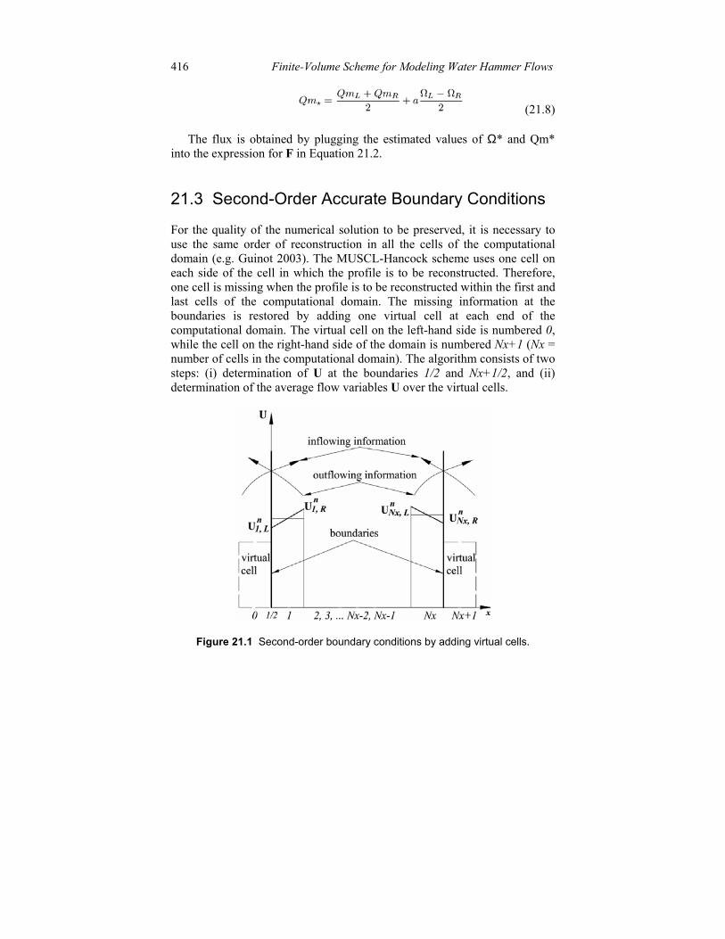
For the quality of the numerical solution to be preserved, it is necessary to use the same order of reconstruction in all the cells of the computational domain (e.g. Guinot 2003). The MUSCL-Hancock scheme uses one cell on each side of the cell in which the profile is to be reconstructed. Therefore, one cell is missing when the profile is to be reconstructed within the first and last cells of the computational domain. The missing information at the boundaries is restored by adding one virtual cell at each end of the computational domain. The virtual cell on the left-hand side is numbered 0, while the cell on the right-hand side of the domain is numbered Nx+1 (Nx = number of cells in the computational domain). The algorithm consists of two steps: (i) determination of U at the boundaries 1/2 and Nx+1/2, and (ii) determination of the average flow variables U over the virtual cells.
Figure 21.1 Second-order boundary conditions by adding virtual cells.

Finite-Volume Scheme for Modeling Water Hammer Flows 417
21.3.1 Determination of Flow Variables at the Boundaries
It is assumed that the average flow variables in the cells 0 to Nx+1 are known from the previous time step and that a second-order reconstruction has been carried out in the cells 1 and Nx (Figure 21.1). The unknown boundary flow variables (Ub) are determined using the theory of Riemann invariants. The reader is referred to Leveque 2002 for a deeper discussion on this theory. The generalized Riemann invariants for water hammer flows (neglecting convective terms) are given by (e.g. Guinot 2003):
(21.9)
Due to space limitations, only the procedure to compute the flux at the left-hand boundary is provided in this section. However, the algorithm is very similar for the right-hand boundary. The left-hand boundary (b) is connected to the left of the first cell (1,L) along the characteristic dx/dt = - am (Figure 21.2).
Figure21.2 Path of integration at left-hand boundary.
Thus, for the left-hand boundary, the second relationship of Equation 21.9 is integrated between b and 1,L, which integration leads to the following relation:
418 Finite-Volume Scheme for Modeling Water Hammer Flows
(21.10)
Another relationship is available from the boundary condition.
(21.11)
Depending on the type of boundary condition imposed, it may or may not be necessary to use an iterative technique to solve the system of Equations 21.10 and 21.11. For instance, let's consider that the pressure is prescribed at the left-hand boundary (pb). This is equivalent to prescribing a mass per unit length Ωb, computed from Equation 21.4.
(21.12)
Since Ωb is known, Qmb can be determined from Equation 21.10. Once Ωb, Qmb, and Af pb are known, the flux at the left-hand boundary Fb = F1/2 can be computed by using the flux relation in Equation 21.2.
21.3.2 Determination of U in the Virtual Cells
Virtual cells are used only to achieve second-order accuracy in the first and last cells of the computational domain. Therefore, they should maintain the conservation property of the FV scheme. The latter means that no unphysical perturbations into the computational domain may be introduced by the virtual cells. These constraints may be satisfied: (i) by assuming that the outflowing wave strengths in the virtual cells are the same as those at the boundaries, and (ii) by adjusting the inflowing wave strengths in the virtual cells in such a way that the fluxes in these cells are the same as those at the respective boundaries. For the left hand boundary, a simple formulation that satisfies these two conditions is given by (Guinot 2003):
(21.13)

Finite-Volume Scheme for Modeling Water Hammer Flows 419
Note that the inflowing and outflowing fluxes in the cell 0 are the same, which means that no perturbations are introduced from the virtual cells into the computational domain when updating the solution. Notice also that with this formulation, the outflowing information advected by the virtual cells is the same as that at the boundaries.
21.4 Evaluation of the Model
The numerical efficiency of the proposed scheme is tested against the second-order FV scheme of Zhao and Ghidaoui (2004), and the fixed-grid MOC scheme with space-line interpolation. These schemes are chosen for comparison because the first one is highly efficient and the second one currently is the most popular approach for modeling water hammer transients. Three test cases are considered in this section. These are:
1. Gradual and partial downstream gate closure in africtionless horizontal pipe.
2. Instantaneous downstream gate closure in a frictionlesshorizontal pipe.
3. Instantaneous downstream gate closure in a pipe withfriction.
The proposed approach is valid for pipes with and without friction. In the two first tests, frictionless pipes are used only because in such cases the physical dissipation is zero, so any dissipation or amplification in the results is solely due to the numerical scheme.
In the following sections, the number of grids, grid size and Courant number used in each example are indicated in the relevant figures and thus will not be repeated in the text. The CPU times that are reported in this chapter were averaged over three realizations and computed using a HP AMD Athlon ™ 64 processor 3200 + 997 MHz, 512 MB of Ram notebook.
21.4.1 Test 1
This test is used to compare the numerical efficiency of the proposed scheme with the second-order scheme of Zhao and Ghidaoui (2004) and the fixed-grid MOC scheme with space-line interpolation for smooth transients (i.e., flows that do not present discontinuities). It is recalled that these schemes are chosen for comparison because the first one is highly efficient and the second one currently is the most popular approach for modeling water

420 Finite-Volume Scheme for Modeling Water Hammer Flows
hammer transients. The test considers one horizontal frictionless pipe connected to an upstream reservoir and a downstream gate. Because of the absence of friction, any dissipation or amplification in the results is solely due to the numerical scheme. The length of the pipe is 10000 m and its diameter is 1.0 m, the pressure-wave celerity is 1000 m/s, the upstream reservoir constant head h0 is 200 m, and the initial steady-state discharge is 2.0 m3/s. The transient flow is obtained after a gradual and partial closure of the downstream gate. For simplicity, this gate is ideally operated in such a way that the flow discharge at the gate is given by the following relationship:
Notice that after a gate is partially closed, the flow discharge at the gate is not constant but oscillates with the same frequency of the water hammer flow until steady state is reached. In this test, for simplicity, after the gate is partially closed, a constant discharge is enforced at the gate, which in a real case would correspond, for instance, to fluctuating the opening of the gate with the same frequency as the water hammer flow. However, the results presented in this section are valid as long as the resulting flow corresponds to a smooth transient.
As suggested by Ghidaoui et al. (1998), the energy equation of Karney (1990) can be used to obtain a quantitative measure of numerical dissipation. The energy equation states that the total energy (sum of internal and kinetic) can only change as work is done on the fluid in the conduit or as energy is dissipated from it. In this test the friction is set to zero, so the rate of total energy dissipation is zero. Thus, any dissipation is solely due to the numerical artifacts. At the downstream boundary, fluid is exchanged with the environment across a pressure difference; therefore work is produced at this boundary. At the upstream boundary, the head at the reservoir is the same as the head after the transient flow has reached steady state. Thus, no work is produced at the upstream end of the pipe (see Karney 1990). Because work is produced at the downstream boundary, the total energy (sum of kinetic and internal) is not invariant with time. Rather it changes periodically with time.
Figure 21.3 shows relative energy traces for the schemes under consideration. The relative energy is expressed as (E - Es)/(E0p - Es), where E0p is the total energy after the flow discharge at the gate is constant

Finite-Volume Scheme for Modeling Water Hammer Flows 421
(e.g. first energy peak in Figure 21.3), Es is the total energy after flow has reached steady state (i.e., by numerical dissipation) and E is the total energy at any time. Figure 21.3 shows clearly a reduction in the relative energy as the gate is gradually closed until the flow discharge at the gate is constant (t = 20 s). For t > 20 s, the energy plot changes periodically with the same frequency of the water hammer flow. If numerical dissipation would be zero, the energy peaks in Figure 21.3 must be maintained. Thus, the numerical dissipation (numerical error) can be obtained as follows:
(21.14)
In this way, if E = E0p there is no numerical dissipation. Likewise, if E = Es (steady state), the numerical dissipation is 100 %. The evaluation of E is made at the ninth energy peak in Figure 21.3 (t ≈ 370 s).
Figure 21.3 Energy traces for test No 1 (Nx = 40 cells, ∆x = 250 m, Cr = 0.8).
To compare the efficiency of the schemes, the numerical dissipation is plotted against the number of grids on log-log scale and shown in Figure 21.4. In this figure, the reduction in numerical dissipation when the number of grids is increased can be approximated as piecewise linear (on log-log scale). Therefore, for a range of Nx, the relationship between
422 Finite-Volume Scheme for Modeling Water Hammer Flows
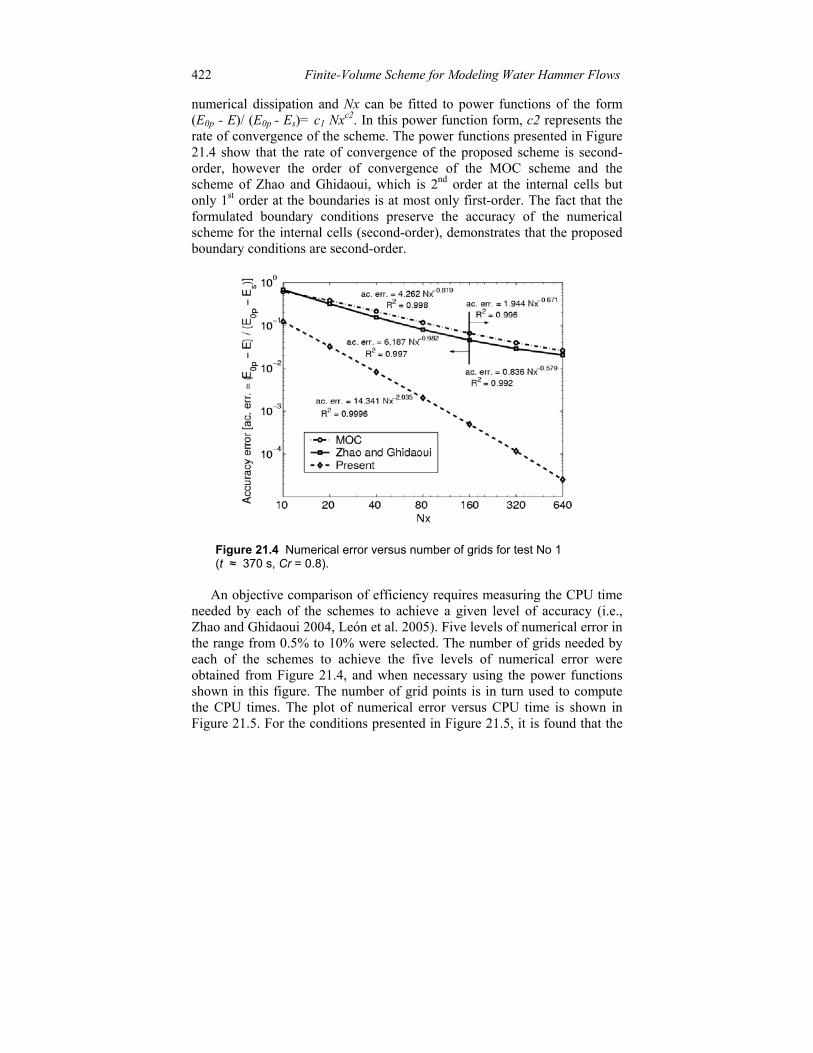
numerical dissipation and Nx can be fitted to power functions of the form (E0p - E)/ (E0p - Es)= c1 Nxc2. In this power function form, c2 represents the rate of convergence of the scheme. The power functions presented in Figure 21.4 show that the rate of convergence of the proposed scheme is second-order, however the order of convergence of the MOC scheme and the scheme of Zhao and Ghidaoui, which is 2nd order at the internal cells but only 1st order at the boundaries is at most only first-order. The fact that the formulated boundary conditions preserve the accuracy of the numerical scheme for the internal cells (second-order), demonstrates that the proposed boundary conditions are second-order.
Figure 21.4 Numerical error versus number of grids for test No 1 (t ≈ 370 s, Cr = 0.8).
An objective comparison of efficiency requires measuring the CPU time needed by each of the schemes to achieve a given level of accuracy (i.e., Zhao and Ghidaoui 2004, León et al. 2005). Five levels of numerical error in the range from 0.5% to 10% were selected. The number of grids needed by each of the schemes to achieve the five levels of numerical error were obtained from Figure 21.4, and when necessary using the power functions shown in this figure. The number of grid points is in turn used to compute the CPU times. The plot of numerical error versus CPU time is shown in Figure 21.5. For the conditions presented in Figure 21.5, it is found that the

Finite-Volume Scheme for Modeling Water Hammer Flows 423
proposed scheme is about 9 to 2100 times faster to execute than the MOC scheme, and 10 to 15200 times faster than the scheme of Zhao and Ghidaoui. The difference in efficiency between the proposed scheme and the other two schemes increases exponentially with the level of accuracy.
Figure 21.5 Relation between level of accuracy and CPU time for test No 1 (t = 370 s, Cr = 0.8).
21.4.2 Test 2
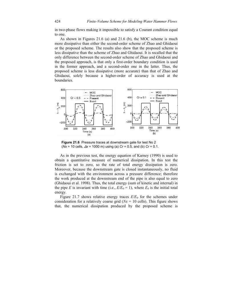
This test is used to compare the accuracy and numerical efficiency of the proposed scheme with the other schemes under consideration for strong transient flows (i.e., flows that do present discontinuities). The test rig is the same as the previous test, except that in this case, the transient flow is obtained after an instantaneous closure of the downstream gate. A portion of the simulated pressure traces for the resulting transient as simulated by the schemes under consideration using a coarse grid (Nx = 10 cells) for Cr = 0.5 and Cr = 0.1 are shown in Figures 21.6 (a) and 21.6 (b), respectively. Additional simulations were performed using a Cr = 1.0. As expected, all schemes under consideration have reproduced the analytical solution when Cr = 1.0 (For clarity, results are not shown). A very coarse grid was used only to illustrate better the benefit of the proposed scheme over the other schemes under consideration for Cr < 1.0. The reason of using low Courant numbers in the present test is because conduits in large systems tend to have different lengths and pressure wave celerities can be very different specially
424 Finite-Volume Scheme for Modeling Water Hammer Flows
in two-phase flows making it impossible to satisfy a Courant condition equal to one.
As shown in Figures 21.6 (a) and 21.6 (b), the MOC scheme is much more dissipative than either the second-order scheme of Zhao and Ghidaoui or the proposed scheme. The results also show that the proposed scheme is less dissipative than the scheme of Zhao and Ghidaoui. It is recalled that the only difference between the second-order scheme of Zhao and Ghidaoui and the proposed approach, is that only a first-order boundary condition is used in the former approach, and a second-order one in the latter. Thus, the proposed scheme is less dissipative (more accurate) than that of Zhao and Ghidaoui, solely because a higher-order of accuracy is used at the boundaries.
Figure 21.6 Pressure traces at downstream gate for test No 2 (Nx = 10 cells, ∆x = 1000 m) using (a) Cr = 0.5, and (b) Cr = 0.1.
As in the previous test, the energy equation of Karney (1990) is used to obtain a quantitative measure of numerical dissipation. In this test the friction is set to zero, so the rate of total energy dissipation is zero. Moreover, because the downstream gate is closed instantaneously, no fluid is exchanged with the environment across a pressure difference; therefore the work produced at the downstream end of the pipe is also equal to zero (Ghidaoui et al. 1998). Thus, the total energy (sum of kinetic and internal) in the pipe E is invariant with time (i.e., E/E0 = 1), where E0 is the initial total energy.
Figure 21.7 shows relative energy traces E/E0 for the schemes under consideration for a relatively coarse grid (Nx = 10 cells). This figure shows that, the numerical dissipation produced by the proposed scheme is
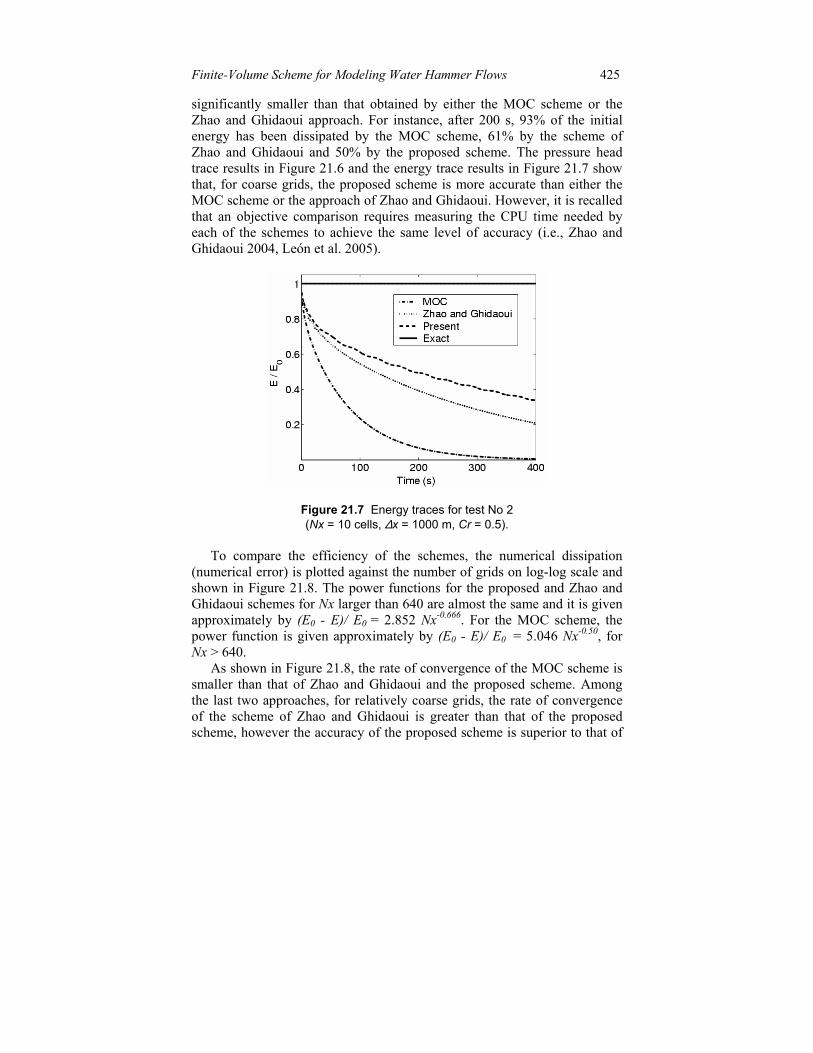
Finite-Volume Scheme for Modeling Water Hammer Flows 425
significantly smaller than that obtained by either the MOC scheme or the Zhao and Ghidaoui approach. For instance, after 200 s, 93% of the initial energy has been dissipated by the MOC scheme, 61% by the scheme of Zhao and Ghidaoui and 50% by the proposed scheme. The pressure head trace results in Figure 21.6 and the energy trace results in Figure 21.7 show that, for coarse grids, the proposed scheme is more accurate than either the MOC scheme or the approach of Zhao and Ghidaoui. However, it is recalled that an objective comparison requires measuring the CPU time needed by each of the schemes to achieve the same level of accuracy (i.e., Zhao and Ghidaoui 2004, León et al. 2005).
Figure 21.7 Energy traces for test No 2 (Nx = 10 cells, ∆x = 1000 m, Cr = 0.5).
To compare the efficiency of the schemes, the numerical dissipation (numerical error) is plotted against the number of grids on log-log scale and shown in Figure 21.8. The power functions for the proposed and Zhao and Ghidaoui schemes for Nx larger than 640 are almost the same and it is given approximately by (E0 - E)/ E0 = 2.852 Nx-0.666. For the MOC scheme, the power function is given approximately by (E0 - E)/ E0 = 5.046 Nx-0.50, for Nx > 640.
As shown in Figure 21.8, the rate of convergence of the MOC scheme is smaller than that of Zhao and Ghidaoui and the proposed scheme. Among the last two approaches, for relatively coarse grids, the rate of convergence of the scheme of Zhao and Ghidaoui is greater than that of the proposed scheme, however the accuracy of the proposed scheme is superior to that of

426 Finite-Volume Scheme for Modeling Water Hammer Flows
Zhao and Ghidaoui. For relatively fine grids, the rate of convergence of the scheme of Zhao and Ghidaoui converges to that of the proposed scheme, and the accuracy of the proposed scheme converges to that of Zhao and Ghidaoui. It was pointed out previously that the proposed scheme is less dissipative (more accurate) than that of Zhao and Ghidaoui, solely because a second-order boundary condition is used in the proposed approach and only a first-order boundary condition in the scheme of Zhao and Ghidaoui. The last two sentences imply that when a large number of grids is used, the effect of the order of accuracy used at the boundary condition becomes negligible.
Figure 21.8 Numerical error versus number of grids for test No 2 (t = 400 s, Cr = 0.5).
The reader can notice that the rate of convergence of the schemes under consideration is not even first-order (0.67 for the proposed and Zhao and Ghidaoui schemes and 0.50 for the MOC scheme). This is because of the presence of discontinuities in the solution (strong transients), in which case a second-order Total Variation Diminishing (TVD) method is at most first-order accurate at the discontinuity regions (i.e., LeVeque 1990). The maximum rate of convergence, which usually is used to name the order of accuracy of a scheme is achieved when applying the scheme to the solution of smooth transients. The order of rate of convergence of the proposed scheme for smooth transients is second order (Test 1). Thus, the proposed scheme is second-order away from discontinuity regions and automatically reverts to first-order at discontinuities.
Finite-Volume Scheme for Modeling Water Hammer Flows 427
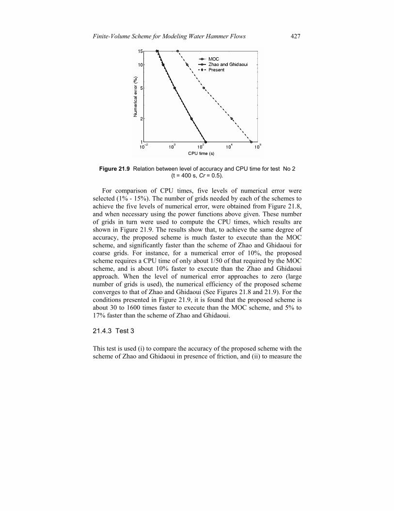
Figure 21.9 Relation between level of accuracy and CPU time for test No 2 (t = 400 s, Cr = 0.5).
For comparison of CPU times, five levels of numerical error were selected (1% - 15%). The number of grids needed by each of the schemes to achieve the five levels of numerical error, were obtained from Figure 21.8, and when necessary using the power functions above given. These number of grids in turn were used to compute the CPU times, which results are shown in Figure 21.9. The results show that, to achieve the same degree of accuracy, the proposed scheme is much faster to execute than the MOC scheme, and significantly faster than the scheme of Zhao and Ghidaoui for coarse grids. For instance, for a numerical error of 10%, the proposed scheme requires a CPU time of only about 1/50 of that required by the MOC scheme, and is about 10% faster to execute than the Zhao and Ghidaoui approach. When the level of numerical error approaches to zero (large number of grids is used), the numerical efficiency of the proposed scheme converges to that of Zhao and Ghidaoui (See Figures 21.8 and 21.9). For the conditions presented in Figure 21.9, it is found that the proposed scheme is about 30 to 1600 times faster to execute than the MOC scheme, and 5% to 17% faster than the scheme of Zhao and Ghidaoui.
21.4.3 Test 3
This test is used (i) to compare the accuracy of the proposed scheme with the scheme of Zhao and Ghidaoui in presence of friction, and (ii) to measure the
428 Finite-Volume Scheme for Modeling Water Hammer Flows
relative magnitude of numerical and physical dissipation. The wall friction is modeled using the modified formula of Brunone by Vítkovsky et al. (2000).
(21.15)
where fq is the Darcy-Weisbach friction factor, u denotes velocity, k is the Brunone’s friction coefficient, and sign(u) = +1 for u ≥ 0 or –1 for u < 0.
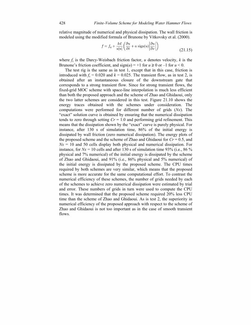
The test rig is the same as in test 1, except that in this case, friction is introduced with fq = 0.020 and k = 0.025. The transient flow, as in test 2, is obtained after an instantaneous closure of the downstream gate that corresponds to a strong transient flow. Since for strong transient flows, the fixed-grid MOC scheme with space-line interpolation is much less efficient than both the proposed approach and the scheme of Zhao and Ghidaoui, only the two latter schemes are considered in this test. Figure 21.10 shows the energy traces obtained with the schemes under consideration. The computations were performed for different number of grids (Nx). The “exact” solution curve is obtained by ensuring that the numerical dissipation tends to zero through setting Cr = 1.0 and performing grid refinement. This means that the dissipation shown by the “exact” curve is purely physical. For instance, after 130 s of simulation time, 86% of the initial energy is dissipated by wall friction (zero numerical dissipation). The energy plots of the proposed scheme and the scheme of Zhao and Ghidaoui for Cr = 0.5, and Nx = 10 and 50 cells display both physical and numerical dissipation. For instance, for Nx = 10 cells and after 130 s of simulation time 93% (i.e., 86 % physical and 7% numerical) of the initial energy is dissipated by the scheme of Zhao and Ghidaoui, and 91% (i.e., 86% physical and 5% numerical) of the initial energy is dissipated by the proposed scheme. The CPU times required by both schemes are very similar, which means that the proposed scheme is more accurate for the same computational effort. To contrast the numerical efficiency of these schemes, the number of grids needed by each of the schemes to achieve zero numerical dissipation were estimated by trial and error. These numbers of grids in turn were used to compute the CPU times. It was determined that the proposed scheme required 20% less CPU time than the scheme of Zhao and Ghidaoui. As is test 2, the superiority in numerical efficiency of the proposed approach with respect to the scheme of Zhao and Ghidaoui is not too important as in the case of smooth transient flows.
Finite-Volume Scheme for Modeling Water Hammer Flows 429
Figure 21.10 Energy traces showing both numerical and physical dissipation.
21.5 Conclusions
This chapter focuses on the formulation and assessment of a FV-based second-order accurate shock-capturing scheme for modeling water hammer flows. The key results are as follows:
1. Numerical tests show that the proposed second-orderformulation at boundary conditions (achieved by using virtual cells) is second-order. In addition, the proposed formulation maintains the conservation property of FV schemes and introduces no unphysical perturbations into the computational domain.
2. Numerical tests were performed for smooth (i.e., flowsthat do not present discontinuities) and sharp transients. The results show that the efficiency of the proposed scheme is superior to both the MOC scheme and the second-order FV scheme of Zhao and Ghidaoui.
3. The high efficiency of the proposed scheme is importantfor RTC of water hammer flows in large networks.
Acknowledgments
The first, third and fourth authors wish to thank the financial support of the Metropolitan Water Reclamation District of Greater Chicago (Research
430 Finite-Volume Scheme for Modeling Water Hammer Flows
Project Specification RPS-03). The second author wishes to thank the Research Grant Council of Hong Kong Grant No. HKUST6113/03E.
References Chaudhry, M. H., and Hussaini, M. Y. (1985). “Second-order accurate explicit finite-
difference schemes for water hammer analysis.” J. Fluids Eng., 107, 523-529. Ghidaoui, M. S., and Karney, B. W. (1994). “Equivalent differential equations in fixed-
grid characteristics method.” J. Hydraul. Eng., 120(10), 1159-1175. Ghidaoui, M. S., Karney, B. W., and McInnis, D. A. (1998). “Energy estimates for
discretization errors in water hammer problems.” J. Hydraul. Eng., 124(4), 384-393. Ghidaoui, M. S., Zhao M., McInnis, D. A., and Axworthy, D. H. (2005). “A review of
water hammer theory and practice.” Applied Mechanics Review, ASME, 58(1), 49-76.
Guinot, V. (2000). “Riemann solvers for water hammer simulations by Godunov method.” Int. J. Numer. Methods Eng., 49, 851-870.
Guinot, V. (2003). Godunov-type schemes, Elsevier Science B.V., Amsterdam, The Netherlands.
Hwang, Y-H., and Chung, N-M. (2002). “A fast Godunov method for the water hammer problem.” Int. J. Numer. Meth. Fluids, 40, 799-819.
Karney, B. W. (1990). “Energy relations in transient closed-conduit flow.” J. Hydraul. Eng., 116(10), 1180-1196.
León A. S., Ghidaoui, M. S., Schmidt, A. R., and García M. H. (2005). “Importance of numerical efficiency for real time control of transient gravity flows in sewers.” Proc., XXXI IAHR Congress, Seoul, Korea.
León A. S., Ghidaoui, M. S., Schmidt, A. R., and García M. H. (2006). “Godunov-type solutions for transient flows in sewers.” J. Hydraul. Eng., 132(8), 800-813.
LeVeque, R. J. (1990). Numerical methods for conservation laws, Birkhäuser Verlag Press, Basel.
LeVeque, R. J. (2002). Finite volume methods for hyperbolic problems, Cambridge University Press, Cambridge.
Szymkiewicz, R., and Mitosek, M. (2004). “Analysis of unsteady pipe flow using the modified finite element method.” Commun. in Numer. Meth. in Eng., 21(4), 183-199.
Toro, E. F. (2001). Shock-capturing methods for free-surface shallow flows, John Wiley and Sons, Chichester.
Vitkosky, J. P., Lambert, M. F., Simpson, A. R., and Bergant, A. (2000). “Advances in unsteady friction modeling in transient pipe flow.” Proc., 8th Int. Conf. on Pressure Surges, A. Anderson, ed., The Hague (NL), bHrGroup, 471-481.
Wood, D. J., Lingireddy, S., Boulos, P. F., Karney, B. W., and McPherson, D. L. (2005). “Numerical methods for modeling transient flow in distribution systems.” J. of the American Water Works Association, 97(7), 104-115.
Wylie, E. B., and Streeter, V. L. (1993). Fluid transient in systems, Prentice-Hall, Englewood Cliffs, N.J.
Zhao, M., and Ghidaoui M. S. (2004). “Godunov-type solutions for water hammer flows.” J. Hydraul. Eng., 130(4), 341-348