compressible flow modeling with combustion engine...
TRANSCRIPT
Master of Science Thesis in Electrical EngineeringDepartment of Electrical Engineering, Linköping University, 2017
Compressible FlowModeling with CombustionEngine Applications
Carl Vilhelmsson

Master of Science Thesis in Electrical Engineering
Compressible Flow Modeling with Combustion Engine Applications
Carl Vilhelmsson
LiTH-ISY-EX--17/5055--SE
Supervisor: Robin Holmbomisy, Linköpings University
Samuel AlfredssonVolvo Car Corporation
Marcus RubenssonVolvo Car Corporation
Examiner: Professor Lars Erikssonisy, Linköping University
Division of Vehicular SystemsDepartment of Electrical Engineering
Linköping UniversitySE-581 83 Linköping, Sweden
Copyright © 2017 Carl Vilhelmsson

Abstract
The high demands on low fuel consumption and low emissions on the combus-tion engines of both today, and the future, is highly dependent on advanced con-trol systems in order to fulfill these demands. The control systems and strategiesare based on models which describe the physical system. The more accuratlythe models describe the real world system, the more accurate the control will be,leading to better fuel economy and lower emissions.
This master’s thesis investigates and improves the mass flow model used for acompressible restriction, such as over the throttle valve, egr valve, or the waste-gate valve, for example. The standard model is evaluated and an improvement isproposed which does not assume isentropic flow. This seems to explain the devia-tion from the isentropic Ψ -function shown in earlier research such as (Andersson,2005). Furthermore a throttle valve is analyzed in ansys in order to show the gen-eration of entropy. The presence of pressure pulsations in a combustion engineis also evaluated, especially how they effect the otherwise assumed steady flowmodel. It is tested if a mean value pressure is sufficient or if one needs to take thepulsations in to account, and the result shows that a mean pressure is sufficient,at least for the throttle when typical intake manifold pulsations is present. Adynamic flow model is also derived which can be useful for pressure ratios closeto one. The dynamic flow model is based on the standard equation but with anextra dynamic term, however it is not implemented and tested due to complexityand time limitation. The proposed new non-isentropic flow model has provenpromising and can hopefully lead to lower emissions and better fuel economy.
iii


Acknowledgments
First of I would like to express my gratitude to Lars Eriksson at vehicular system,Linköping University and the air charge group at Volvo Car Corporation whichbrought this subject to my attention and gave me the opportunity to conduct thismaster’s thesis. Furthermore i would like to thank my supervisor at LinköpingUniversity, Robin Holmbom for his guidance and the productive discussions wehad. I also want to send a thank to my supervisors at Volvo Car Corporation,Samuel Alfredsson and Marcus Rubensson which have shown great interest andhave helped me a lot with supplying me with data and answering questions. Athank also goes out to Tobias Lindell working at the engine lab at Vehicular Sys-tems, Linköping University, helping me with for instance collecting data andinstalling new sensors on the engine rig.
Linköping, june 2017Carl Vilhelmsson
v


Contents
1 Introduction 11.1 Background . . . . . . . . . . . . . . . . . . . . . . . . . . . . . . . 11.2 Problem Formulation . . . . . . . . . . . . . . . . . . . . . . . . . . 21.3 Expected Results . . . . . . . . . . . . . . . . . . . . . . . . . . . . . 31.4 Outline . . . . . . . . . . . . . . . . . . . . . . . . . . . . . . . . . . 4
2 Related Research 52.1 Common Fluid Science . . . . . . . . . . . . . . . . . . . . . . . . . 52.2 Incompressible Flow Restriction . . . . . . . . . . . . . . . . . . . . 62.3 Compressible Flow Restriction . . . . . . . . . . . . . . . . . . . . . 62.4 Pressure Pulsations . . . . . . . . . . . . . . . . . . . . . . . . . . . 72.5 Applications for the Flow Model . . . . . . . . . . . . . . . . . . . . 9
2.5.1 Wastegate . . . . . . . . . . . . . . . . . . . . . . . . . . . . 92.5.2 Throttle and EGR . . . . . . . . . . . . . . . . . . . . . . . . 102.5.3 Turbo . . . . . . . . . . . . . . . . . . . . . . . . . . . . . . . 102.5.4 Cylinder Air Charge . . . . . . . . . . . . . . . . . . . . . . 11
3 Theory and Phenomena 133.1 Steady Isentropic Compressible Flow . . . . . . . . . . . . . . . . . 133.2 Steady Non-Isentropic Compressible Flow . . . . . . . . . . . . . . 163.3 Pulsating Pressure Ratio . . . . . . . . . . . . . . . . . . . . . . . . 203.4 Unsteady Isentropic Compressible Flow . . . . . . . . . . . . . . . 21
4 Approach 254.1 Steady Compressible Flow . . . . . . . . . . . . . . . . . . . . . . . 26
4.1.1 Approach . . . . . . . . . . . . . . . . . . . . . . . . . . . . . 264.1.2 Measurements . . . . . . . . . . . . . . . . . . . . . . . . . . 27
4.2 Unsteady Compressible Flow . . . . . . . . . . . . . . . . . . . . . 284.2.1 Approach . . . . . . . . . . . . . . . . . . . . . . . . . . . . . 284.2.2 Measurements . . . . . . . . . . . . . . . . . . . . . . . . . . 30
5 Results 315.1 Fixed Throttle Position . . . . . . . . . . . . . . . . . . . . . . . . . 31
vii

viii Contents
5.2 Normal and Extended Ψ -function . . . . . . . . . . . . . . . . . . . 325.2.1 Engine Measurements . . . . . . . . . . . . . . . . . . . . . 325.2.2 Flow Bench Measurements . . . . . . . . . . . . . . . . . . . 35
5.3 Pulsating Pressure Ratio . . . . . . . . . . . . . . . . . . . . . . . . 385.4 Throttle Valve ANSYS Analysis . . . . . . . . . . . . . . . . . . . . 425.5 Dynamic Compressible Flow . . . . . . . . . . . . . . . . . . . . . . 45
6 Conclusion 536.1 Summary . . . . . . . . . . . . . . . . . . . . . . . . . . . . . . . . . 536.2 Future Work . . . . . . . . . . . . . . . . . . . . . . . . . . . . . . . 55
6.2.1 Ψ -function . . . . . . . . . . . . . . . . . . . . . . . . . . . . 556.2.2 Dynamic Flow Model . . . . . . . . . . . . . . . . . . . . . . 55
A Calculations for Isentropic Compressible Flow 59
B Calculations for Non-isentropic Compressible Flow 63
C Calculations for Unsteady Compressible Flow 67
Bibliography 71
Contents ix
Parameters and Variables
Notation Description
p Pressure [pa]T Temperature [K]m Mass flow [kg/sec]R Gas constant air [-]γ Ratio of specific heats air [-]ρ Density [kg/m3]V Velocity [m/s]h Enthalpy [KJ/Kg]cp Specific heat constant pressure [kJ/kgK]cv Specific heat constant volume [kJ/kgK]s Entropy [kJ/kgK]
Abbreviations
Abbreviations Description
vcc Volvo Car Corporationvnt Variable Nozzle Turbinepid Proportional Integral Derivateivecfd Computational Fluid Dynamicsmvem Mean Value Engine Modelegr Exhaust Gas Recyclingmatlab Calculation programsimulink Simulation programansys Finite element method calculation programfiltfilt Filtering function in matlab
lsqcurvefit Least square function in matlab

x Contents

1Introduction
A short introduction to the problems and why it is interesting to investigate themfurther is presented in this chapter. The main goals and the primary expectedresults of the thesis along with the outline is also introduced here.
1.1 Background
Today’s vehicles have to be more and more environmentally friendly, one of themain effects a vehicle has on the environment is the release of greenhouse gasescoming from the burning of fossil fuel. To reduce this effect and save money theconsumer wants fuel efficient vehicles. In order to design and control these newengines, models for each component are required to be accurate and reliable inall driving situations. Some of these components are the different valves whichdirects flows in the engine, such as the throttle, egr, and wastegate. One aspectthat has not been investigated is the effect of pulsations for both low and highpressure ratios.
One example is the wastegate, a bypass valve that controls how much of theexhaust flow goes in to the turbocharger thereby boosting the engine with air lead-ing to better fuel economy. The wastegate flow model is not well developed dueto the harsh and unsteady conditions in the exhaust, making it hard to measurethe flow and get an accurate model for all working conditions. The model for thewastegate effects the whole engine simulation model. Some of the obvious bene-fits of having an accurate model is that together with a turbocharger model onecan apply a good feed forward to the boost control loop increasing driveability.An accurate model will estimate the exhaust manifold pressure more correctlywhich affect the calculations for volumetric efficiency, hence correct air fuel ratiowill be obtained and lower emissions achieved. This master’s thesis will addresssome different flow phenomena, pulsating and unsteady flow, low and high pres-
1
2 1 Introduction
sure ratios over restrictions and hopefully end up with an extended useful modelfor mass flow through a compressible restriction.
1.2 Problem Formulation
Accurate and faster engine control systems are one way to increase fuel economy,driveability, and decrease emissions. For this, better models of the different com-ponents in the engine are needed. The wastegate can be seen as a compressible re-striction, just as the throttle, and in some cases the egr-valve. There are two maintypes of egr systems, low pressure route, and high pressure route. High pressureroute can be seen as a compressible restriction but the low pressure route egr-valve have to be investigated further. There are several problems when tryingto model the wastegate and egr flow. When using the same analogy as for thethrottle, measuring the mass flow can not be done due to the heat which a regularmass flow meter can not handle, and for the egr the pulsating flow sometimesleads to back flow. The fact that the mass flow is split up between the turbine andthe wastegate makes the mass flow meter on the intake side of the engine unus-able in order to obtain the mass flow past the wastegate. The pulsations comingfrom the cylinder when an exhaust valve opens makes the pressure ratio over thewastegate not to be steady which is assumed in the throttle case. There might alsobe flow disturbances and circulations occurring due to the fact that wastegate andturbine is located so close to each other. Some previous works such as Andersson(2005),Hendricks et al. (1996) have shown that the model used, based on isen-tropic compressible flow does not correspond with measured data see figure 1.1.That model is then adapted to fit the measured data in many different ways, somedifferent ideas are proposed by for example (Hendricks et al., 1996)(ReshapingΨ (Π)-function with help of 2 parameters),(Andersson, 2005)(Uses gamma as tun-able parameter). The interesting part is why it differs from the theory, this willbe investigated further. To be carried out in this thesis are the following:
• 1: Repeat the measurements in (Andersson, 2005) showing that the CdΨ (Π) ,Ψ (Π).
• 2: Investigate with the help of CFD to why these phenomena occurs.
• 3: Investigate the effects pressure pulsations have on the model where theconditions otherwise are assumed steady.
• 4: Create an extended flow model, combining the model for an isentropiccompressible restriction with the previous investigations.
• 5: Investigate the improvements of the new extended model against thebasic model.

1.3 Expected Results 3
Figure 1.1: The original data measured by Per Andersson at vehicular sys-tem, Linköping University is shown in this figure. One can clearly see thedeviation between model and collected data. The original picture comesfrom (Andersson, 2005).
1.3 Expected Results
The main expected result of this thesis is an useful extended model for the massflow through a variable restriction, that can be used for improving the total en-gine model, which would lead to better and more accurate engine control. Thisis obtained by closer investigation of the different sub problems.
• 1: Reconstructed measurements from the work in (Andersson, 2005) show-ing that the theory for an isentropic compressible restriction do not matchthe measurements.
• 2: CFD simulations trying to explain why the deviation in the Ψ (Π)-functionoccurs.
• 3: Plots and data showing the effects a pulsating pressure have on the com-pressible flow model.
• 4: Flow through a variable restriction is measured for different pressuresin a test bench in order to eliminate the effects pulsations have on the massflow and furthermore evaluating what is causing the deviation.

4 1 Introduction
• 5: Taking the results from the previous stated excepted results and devel-oping a new extended mass flow model.
• 6: Presented measurements of the flow through a restriction and comparingthe new extended model against a basic model.
1.4 Outline
The main chapters of this thesis with a short description are as follows:
• Chapter 1 - IntroductionIntroduction to the problem, why it is desirable to solve and expected re-sults
• Chapter 2 - Related ResearchPresenting the literature studies made on the subject.
• Chapter 3 - Theory and PhenomenaDifferent theories and ideas are presented in what manner some problemsare to be solved.
• Chapter 4 - ApproachThis chapter describes how the different tests are to be carried out and whatdata is to be collected and why.
• Chapter 5 - ResultThis presents the results from the different problems and tests stated inprevious chapters.
• Chapter 6 - ConclusionThe conclusions which can be drawn are presented here along with someideas for future work.

2Related Research
Here some related research is presented which were part of the literature studiesconducted in order to form a better understanding of the subject of this master’sthesis. Information is also collected about both common fluid science and wherethese equations can be applied when modeling some engine components is pre-sented here.
2.1 Common Fluid Science
Fluid is the common name for gases and liquids, a fluid’s properties can for exam-ple be described by its viscosity, compression module, and density. These basicproperties are also dependent on the internal states of a fluid, such as pressureand temperature, but can in some cases for simplicity be considered as constants.There are three main governing equations within fluid science, the continuityequation which states the preservation of mass, the momentum equation whichis a form of newtons second law of motion, the energy equation which states thepreservation of energy. When considering a fluid flowing in a pipe one very use-ful dimensionless number is the Reynold’s number which is the relation betweeninertial forces and viscous forces. The Reynold’s number can describe the type offlow, if it is laminar, semi turbulent or fully developed turbulent flow, this is veryuseful when choosing the approach by which a problem is to be solved. Reynold’snumber is described in equation (2.1), where U is the relative fluid velocity, L isthe characteristic length and v is the dynamic viscosity. For a non-circular pipethe characteristic length (L) is the hydraulic diameter (dh), described in equation(2.2) where A is the area of the cross section and O is the circumference. Morebasic fluid science is presented in (Karl Storck, 2012).
5
6 2 Related Research
Re =Inertialf orces
V iscousf orces=ULv
(2.1)
dh =4AO
(2.2)
2.2 Incompressible Flow Restriction
An incompressible flow is a flow where the change in density of the fluid isvery small and can be neglected. Incompressible flow can be described with theBernoulli equation, if friction and compressibility effect are neglected. In (Çengelet al., 2012) the incompressible flow equation is derived from Newton’s secondlaw of motion. The inertia of the gas when reaching high velocities is the reasonthe flow is considered to be compressible, when the velocities are low the inertiacan be neglected, hence incompressible flow. Equations for such flows througha restriction are described in (Eriksson and Nielsen, 2014) both for laminar andturbulent flows. The long route egr-valve can perhaps be seen as an incompress-ible flow since the pressure drop over the valve is low, hence the gas velocity andinertia is low, however in (Klasén, 2016) a compressible flow model is used sinceit produced a slightly better fit to measured data.
2.3 Compressible Flow Restriction
A compressible flow is a flow where the density in the fluid changes significantlyand have to be considered. The flow equations for an isentropic compressiblerestriction with the shape of a converging nozzle, seen in figure 3.1a, are derivedin (Çengel et al., 2012). However, the assumption that these equations apply tothe shape of a throttle shown in figure 3.1b, and also the shapes of wastegate andin some cases EGR valves, are made in many automotive works. This assumptionmight be the reason for the deviation from measured data to theory. Assumingthe flow is isentropic, compressible, and adiabatic a model for the throttle is de-scribed in (Eriksson and Nielsen, 2014). Since it is in this thesis beneficial to havethe Ψ (Π) function normalized, to make it easier to compare with normalizeddata, the normalized model stated in (Andersson, 2005) is to be used. Here alsoa small linear region is added to fulfil the Lipschitz condition, and prevent oscil-lations. An indication that the linear region is to small is if oscillations in massflow occurs during simulations at steady state, stated in (Eriksson and Nielsen,2014).
Together with others, (Andersson, 2005) says that Cd , the discharge coefficient,are mainly dependent on two factors, pressure ratio Π and the valve angle α. Thearea dependent factor Cd(α) is hidden within the model for effective area, as in(Eriksson and Nielsen, 2014), Aef f (α) = Cd(α)A(α), which are determined usingmatlab function lsqcurvfit, hence there is no need to determine Cd(α) solely. Todetermine if the pressure ratio dependent factor of Cd(Π) is negligible, (Ander-sson, 2005) plots Cd(Π)Ψ (Π) together with only the Ψ (Π)-function and here a
2.4 Pressure Pulsations 7
deviation occurs which implies that Cd(Π) can not be ignored. His test is carriedout by setting a throttle valve at a fixed position and doing a sweep in pressureratio, which is done by controlling the engine speed. Furthermore the data isnormalized by dividing with the mean of the three biggest measured values foreach throttle angle, this to remove the area/angle dependent factor. Explained,the biggest values are assumed to be the same as Aef f (α) since Cd(Π)Ψ (Π) is onewhere the biggest values occurs, hence a division removes the effect of Aef f (α).Further explanation on how this is used is described in the approach chapter.
2.4 Pressure Pulsations
In the books (Ockendon, 2003) and (Lighthill, 2001) waves and compressible floware described in detail. Special interest for this thesis are longitudinal waves intubes which can be described using non-linear gas dynamic equations, (2.3). Theassumption that the variables only change along the length of the tube is made,for every cross section area the variables are thus the same. These equations areobtained by solving the governing equations, which are the continuity equation,momentum equation, and energy equation. These equations are described fur-ther in (Yang, 2015) and (Chalet et al., 2011).
∂ϕ
∂t+∂F(ϕ)∂x
= B (2.3a)
ϕ =
ρAρuA
ρ(e + 1
2u2)A
(2.3b)
F(ϕ) =
ρuA
(p + ρu2)A
ρu(e + 1
2u2 + pρ−1
)A
(2.3c)
B =
0p dAdx − ρFrρqeA
(2.3d)
These equations are preferable solved numerically, but analytical solution ex-ists, however they might only apply to specific conditions. One of those solutionsgives the linear acoustic wave equation (2.4), where only small fluctuations inthe thermodynamic properties, pressure and density are considered and all non-linear effects are negligible. The mean velocity is not taken into account, all thisconsidered, these equation are a good, if not perfect description for sound waveswhere all the considerations are true.
∂2pe∂x2 =
1
c20
∂2pe∂t2
(2.4)
8 2 Related Research
The aucustic wave equation is useful when considering sound in the engine,but might not be useful when modelling the high amplitude pressure pulsations,and varying gas speed in the exhaust or intake manifold. In the books mentionedabove there are also models for waves propagating through restrictions, apply-ing the analogy to electrical impedance and inductance. In (Lighthill, 2001) theinductance is described carefully, and some examples for various geometries aregiven, it is to be solved with numerical integration of the Laplace equation forthat specific geometry, or approximated. Which in the case of a variable restric-tion makes it very inconvenient, a map for different areas, pressure ratio overrestriction, and flow would have to be made to get the correct inductance for allcases. This makes the inductance approach, at least in this case, very inconve-nient but for a non-variable restriction and known waves it is useful. Howeverin (Kiwan et al., 2016) an unsteady compressible flow equation is derived whichtakes the inertia of the gas into account, hence making it possible to take the pul-sations and transients into account. This unsteady compressible flow equationseems to estimate the flow much more accurate than the steady compressibleflow equation in (Çengel et al., 2012). (Kiwan et al., 2016) validates the modelagainst "GT power", which is an engine simulation program and not real worlddata, however "GT power" is well recognized among engine manufacturers.
In a combustion engine it is two main type of waves, expansion wave, andcompression wave, the expansion wave is a wave of lower pressure such as inthe intake manifold and the compression wave is a wave of higher pressure suchas in the exhaust manifold. When these waves enters a larger volume or cavitya part of the wave is reflected backwards but as the opposite wave, detailed de-scription in (Lighthill, 2001). For example, a low pressure wave in the intakerunner excited by the opening of the intake valve enters the larger manifold cav-ity and this causes a part of the wave energy to reflect back into the runner asa compression wave. This effect is used when engine designers tune the lengthof the runners so that the reflected compression wave enters the cylinder just be-fore the intake valves are closing. In many works the waves effect are neglectedand only some mean value model is used, however in (Stockar et al., 2016) a wayof modelling the transients and waves are proposed which uses the one dimen-sional wave equations and a reduction methodology to make the equations moremanageable. This wave description together with the unsteady compressible re-striction equation in (Kiwan et al., 2016) can be useful to both model the wavesand calculate their effects on the flow through a restriction. In (Semlitsch et al.,2014) an in depth analysis of the flow leaving the cylinders through the exhaustvalves are made, the approach is numerical with finite elements which do notdirectly help this thesis, but a wider understanding of the different events underwhich gas enters the exhaust manifold are described. There are two main partsunder which gases evacuates the cylinder, the blow-down phase, which occurswhen the exhaust valve first opens and the pressure in the cylinder are rapidlyblown out until pcyl = pem. Part two is when the upward motion of the piston ispushing out the remaining exhaust gases. This is also described in (Eriksson andNielsen, 2014) where the different events also can be seen in a p − V diagram.
The frequencies of the pulsations are shown in previous works such as (Macián

2.5 Applications for the Flow Model 9
et al., 2004) and (Liang and Holmbom, 2016), where measurements of pressurehave been made and proven to be the same as that of the exhaust valves open-ings (2.5). There will also be resonance frequencies due to the exhaust manifoldvolume and length of pipe.
ωp =2RPM
602π (2.5)
In (Thomasson and Eriksson, 2015) a model for the pressure waves in theexhaust manifold are developed, this model assumes exhaust valve as a com-pressible restriction and calculates the cylinder pressure trace. When the exhaustvalves opens the cylinder pressure and temperature are used to calculate the rateof mass flow to the exhaust manifold, hence leading to pressure pulsations in thevolume.
2.5 Applications for the Flow Model
The use of an extended flow model taking the pulsations and dynamic behav-ior into account have many applications where such conditions are present, thisthesis focuses on the valves related to combustion engines such as the throttle,wastegate, and egr valves. In this section a short introduction of the differentvalves, and improvements an accurate flow model can have is described.
2.5.1 Wastegate
When modeling a valve such as the wastegate valve there are two main parts, thesignal to position model, and the position to flow model. More about modelling,both with a system identification approach and a physical modelling approachare described in (Ljung and Glad, 2004).
Flow Model
The flow model is using the above described compressible flow through restric-tion equations, where the Aef f (α) and Cd(Π) are to be found. This assumesthat the discharge coefficient can be divided into two parts one angle depen-dent and one pressure ratio dependent, Cd(α,Π) = Cd(α)Cd(Π). Starting of withthe modelling of the Cd(Π)Ψ (Π)-function one can chose between some differentapproaches described in for example (Andersson, 2005), and (Hendricks et al.,1996). However the idea is the same, normalizing the function to remove areadependent factor and then fitting Cd(Π) so that Cd(Π)Ψ (Π) agrees with measure-ments. When Cd(Π)Ψ (Π) are modeled, the approach in (Eriksson and Nielsen,2014) can be used to model the Aef f using lsqcurvfit to parametrize some poly-nomial function. Measurements are obviously made in order to obtain the datafor fitting the models.

10 2 Related Research
Position Model
The modelling of the positioning in such a valve as the wastegate are carefullydescribed in (Thomasson et al., 2013) with help of, for example (Mehmood et al.,2010) to model the aerodynamic force. First a model for signal to wastegate ac-tuator are made with slow ramps to describe the statics and then steps are madeto evaluate the time constant, there are different time constants depending onif pressure is rising or falling. Furthermore according to Newton’s second lawof motion a force balance is set up (2.6), which is the model for the wastegate’sposition.
xm = Famb − xb − Fact − Ff r − Fsb − Faero (2.6)
An approach by which the different forces are identified is described, firstby static experiment to remove the influence of dynamic friction and the mass,when they are identified steps are made and the mass (m) and dynamic damping(b) are fitted using lsqcurvfit. The aerodynamic force is modeled in (Mehmoodet al., 2010) for a VNT-system but the approach may be the same. The aerody-namic force is mainly dependent on the pressure difference between the exhaustmanifold and the following exhaust. Previous forces are calculated with engineoff to remove the influence of aerodynamic force, when engine is turned on thedifference between the expected static position and the real position are due toaerodynamic force which then can thus be determined. A model for the vacuumtank and pump is also proposed in (Thomasson et al., 2013). However assumingthat the vacuum pump can keep the pressure constant, a vacuum reference pres-sure will suffice. A model for the wastegate position is needed in order to obtain agood feed forward to the turbo control, and be able to evaluate the improvementsof a better flow model.
2.5.2 Throttle and EGR
The throttle and egr valves are very similar in the design but have different pur-poses, throttle controlling the air flow into the engine and the EGR controllinghow much exhaust gases are recycled. Both valves are however butterfly valvescontrolled with a servo motor, the design can be seen in figure 3.1b. The posi-tioning system of these valves are much simpler to model than the positioning ofthe wastegate valve since they are actuated by, in most cases, a closed loop servomotor. In (Eriksson and Nielsen, 2014) a first order system is proposed for thethrottle reference signal to position, a simple step response is sufficient to obtainthe gain and time constant. The flow modeling is furthermore the same as for thewastegate, however a different polynomial function for the effective area (Aef f )might be used to capture the different shape characteristics.
2.5.3 Turbo
The boost pressure control system are greatly dependent on estimation and mod-elling of the turbocharger, which in turn needs an accurate estimation of mass

2.5 Applications for the Flow Model 11
flow through the turbine driving the turbo charger. The difficulty lies here in es-timating how the total mass flow is divided among the turbine and the wastegatepath. If accurate models for wastegate signal to boost pressure are presented afast control system can be developed. First when designing a control system forthe boost pressure, models for the compressor, turbine, and connecting shaft isneeded. In (Eriksson and Nielsen, 2014) basic models for compressor, turbine,and shaft are described, in (Leufvén and Eriksson, 2013) an extension of thesemodels are proposed that is choke and surge capable. Furthermore in (Llamasand Eriksson, 2017) a new way of fitting the data to the models is described,where not the model error is minimized, instead the orthogonal distance to themodel is minimized. In (Leufven and Eriksson, 2016) turbo compressor modelsare extended for low pressure ratios. There are many different approaches onhow to develop a turbo control system depending on such as what sensors areavailable and how much effort is put into the design. In (Eriksson and Nielsen,2014) a static feed forward from a look up table, together with a second orderengine speed dependent system is used. The look up table is the static gain fromwastegate position to boost pressure for different engine speeds, and the secondorder systems are identified with help of step responses, also for different enginespeeds. The regulator parameters, which also are engine speed dependent, aretuned using IMC. In (Criscuolo et al., 2011) a similar approach is made, howeverit is for a two stage sequential turbocharging system and the supply voltage iscompensated for. In (Liang and Holmbom, 2016) a structure where the systemis modeled in different stages are made, here sensors for turbo speed and waste-gate position is supplied. Different solutions are proposed on how to model thesystem for requested boost pressure to requested turbo speed, a look up table,non-linear static compensator, or physical modeling. The turbo speed is thencontrolled instead of controlling the boost pressure directly. Static errors are re-moved by a feedback controller from boost pressure to requested turbo speed.The system from wastegate to turbo speed is then identified by doing step re-sponses and assuming first order system. This way parts of the system can bemodeled separately, and hopefully leading to a better and more complete defini-tive model, due to the fact that less characteristics of different parts are over-looked. In common for most turbo controllers are that they consists of some sortof PID-controller, however there are exceptions, such as in (Liang and Holmbom,2016) where a state feedback is used with an integrating part. Common is alsothe use of kalman filters to estimate states which are of interest. More generalcontrol theory can be read about in (Glad and Ljung, 2006), (Glad and Ljung,2003), and (Martin Enqvist and Strömberg, 2014), for example.
2.5.4 Cylinder Air Charge
The total air mass flow to the cylinder are described in (Andersson, 2005) (2.7),here for one cylinder, which then is used to calculate the correct amount of fuelto be injected. The volumetric efficiency ηvol-function are described in manydifferent works and in many different ways, it is usually a function which isparametrized with regards to engine speed and intake manifold pressure, some

12 2 Related Research
models are proposed in (Eriksson and Nielsen, 2014).
CAC = ηvolpimVdRimTim
(2.7)
There is also the approach of physical modeling where effects as charge cool-ing, residual gases, and fuel enrichment are taken into account. One such model(2.8) are described in (Andersson, 2005), here it is only two tuning parameters,and the ηvol-function is not present.
CAC =pim
Rim
(Tim − C1
1−λ2
λ2
)Cηvol(rc −
(pempim
) 1γe
)Vd(
1 + 1λ( AF )s
)(rc − 1)
(2.8)
A sensitivity function for how the exhaust pressure pem effects the CAC is alsoderived from (2.8) in (Andersson, 2005), which is a good tool when evaluatinghow much the improved estimations of pem due to better wastegate flow model,effects the CAC. In order to compare the improvements of the flow model a base-line exhaust pressure model is required which also is presented in (Andersson,2005).
3Theory and Phenomena
In this chapter the theory and governing equations behind the models used in thismaster’s thesis are presented. The assumptions made when deriving the modelsare explained and ways of improving and investigating why some errors occurare described here.
3.1 Steady Isentropic Compressible Flow
Similar derivation is made in a lots of previous works, one example (Çengel et al.,2012), but the derivation is also presented her in order for the reader to get a bet-ter understanding. In steady flow, a flow where the fluid properties can changefrom point to point, but for every point they do not change with time. The conser-vation of energy equation, with help of the enthalpy describing internal energycan be applied, assuming no work or heat is transfered out, or in to the system.The following equation can be stated:
h1 +V 2
12
+ gz1 = h2 +V 2
22
+ gz2 (3.1)
For an ideal gas the enthalpy is only dependant on the temperature, when assum-ing that the specific heat constant pressure (cp) is a constant, hence the followingequation applies:
h2 − h1 = cp(T2 − T1) (3.2)
Studying the figure 3.1 and assuming that it is only small changes in potential en-ergy, (z1 − z2 ≈ 0). Also assuming that the inlet velocity is very low relative to theexit velocity V 2
2 − V21 ≈ V
22 Combining this assumption with previous equations
(3.1) and (3.2) following equation is obtained:
13
14 3 Theory and Phenomena
� �2
T1
�.
T2
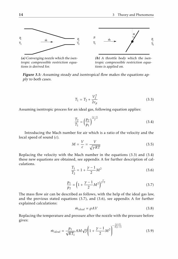
(a) Converging nozzle which the isen-tropic compressible restriction equa-tions is derived for.
��2
T1
�.
α
T2
(b) A throttle body which the isen-tropic compressible restriction equa-tions is applied on.
Figure 3.1: Assuming steady and isentropical flow makes the equations ap-ply to both cases.
T1 = T2 +V 2
22cp
(3.3)
Assuming isentropic process for an ideal gas, following equation applies:
T2
T1=
(p2
p1
) (γ−1)γ
(3.4)
Introducing the Mach number for air which is a ratio of the velocity and thelocal speed of sound (c).
M =Vc
=V√γRT
(3.5)
Replacing the velocity with the Mach number in the equations (3.3) and (3.4)these new equations are obtained, see appendix A for further description of cal-culations.
T1
T2= 1 +
γ − 12
M2 (3.6)
p1
p2=
(1 +
γ − 12
M2) γγ−1
(3.7)
The mass flow air can be described as follows, with the help of the ideal gas law,and the previous stated equations (3.7), and (3.6), see appendix A for furtherexplained calculations:
mideal = ρAV (3.8)
Replacing the temperature and pressure after the nozzle with the pressure beforegives:
mideal =p1√RT1
AM√γ
1 +γ − 1
2M2
−(γ+1)
2(γ−1)
(3.9)

3.1 Steady Isentropic Compressible Flow 15
Substituting the Mach number with pressure ratio (Π), see appendix A, addingthe discharge coefficient (Cd(α,Π)) which we assume is depending on the throt-tle angle and pressure ratio. Also changing the area factor (A) to a function ofthrottle angle (A(α)) seen in figure 3.1b. This sets up for a useful function whenapplied to a variable nozzle, valve, or throttle.
m =p1√RT1
A(α)Cd(α,Π)
√2γγ − 1
(Π
2γ −Π
γ+1γ
)︸ ︷︷ ︸
Ψ (Π)
(3.10)
Where Π is the ratio of pressure over the nozzle if flow is going from pressure oneto pressure two, otherwise the pressure and temperature in the equation have tobe switched so that the ones upstream are used in equation (3.10). Assumingonly one direction of mass flow the pressure ratio are defined as follows:
Π =
p2p1
if p2 < p1
1 otherwise(3.11)
The critical pressure ratio is at the maximum of the Ψ (Π)-function, this happenswhen the speed of sound is reached in the nozzle, this occurs for pressure ratios:
Π =( 2γ + 1
) γγ−1
(3.12)
Using the critical pressure ratio in the Ψ -function we state the normalized Ψ *-function as follows:
Ψ ∗(Π) =
√2γγ−1
(Π
2γ −Π
γ+1γ
)√
2γγ−1
( 2γ+1
) 2γ−1−(
2γ+1
) γ+1γ−1
(3.13)
Applying the linear region in order to fulfil the Lipschitz condition and preventoscillations for pressure ratios near one when simulating, also setting the valuesunder the critical pressure ratios to one. This in order for the model to work in alpossible conditions.
Ψ (Π) =
1 if 0 < Π ≤
(2γ+1
) γγ−1
Ψ ∗(Π) if(
2γ+1
) γγ−1
< Π ≤ Πlin
Ψ ∗(Πlin) Π−1Πlin−1 if Πlin < Π ≤ 1
(3.14)
This function can be seen in the figure 3.2 where the linearized limit is set toΠlin = 0.99 and γ = 1.4.

16 3 Theory and Phenomena
0.2 0.3 0.4 0.5 0.6 0.7 0.8 0.9 1 1.1
Π
0
0.2
0.4
0.6
0.8
1
Ψ*
Normalized Ψ*(Π ) - function
Figure 3.2: Here the Ψ -function for an isentropical compressible nozzle canbe seen with both linearized area for pressure ratios over 0.99, and for pres-sure ratios below the critical ratio the function are set to one.
3.2 Steady Non-Isentropic Compressible Flow
Previous calculations of the expansion and acceleration were based on equation(3.4) which assumes the generated entropy to be zero. Entropy is a state property,entropy is the quantity of microscopic disorder in a system, more informationabout entropy can be found in (Çengel et al., 2012). The change of entropy isdefined as follows:
dS =(dQT
)(3.15)
For an ideal gas where the specific heats are assumed constants, the change inentropy can be described as follows for any process:
s2 − s1 = cv lnT2
T1+ Rln
V1
V2(3.16a)
s2 − s1 = cplnT2
T1− Rln
p2
p1(3.16b)
If the process is assumed to be isentropic (s2 − s1 = 0) the equation (3.16b)gives the previous stated equation (3.4). In figure 3.3, a diagram of the isentropicprocess is shown together with a more accurate process which is called the actualprocess. A logical explanation to the loss of kinetic energy which can be seen inthe diagram is the fact that the molecules bounce and collide lowering the overall
3.2 Steady Non-Isentropic Compressible Flow 17
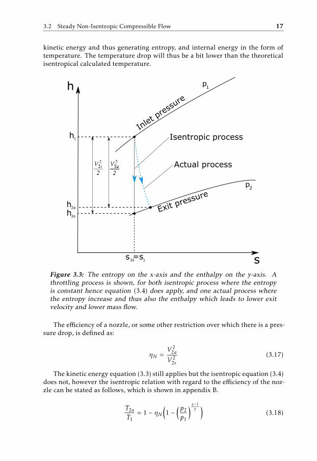
kinetic energy and thus generating entropy, and internal energy in the form oftemperature. The temperature drop will thus be a bit lower than the theoreticalisentropical calculated temperature.
s
h p1
p2
Isentropic process
Actual process
h1
h2a
h2s
s2s=s
1
Inle
t pre
ssur
e
Exit pressu
re
Figure 3.3: The entropy on the x-axis and the enthalpy on the y-axis. Athrottling process is shown, for both isentropic process where the entropyis constant hence equation (3.4) does apply, and one actual process wherethe entropy increase and thus also the enthalpy which leads to lower exitvelocity and lower mass flow.
The efficiency of a nozzle, or some other restriction over which there is a pres-sure drop, is defined as:
ηN =V 2
2a
V 22s
(3.17)
The kinetic energy equation (3.3) still applies but the isentropic equation (3.4)does not, however the isentropic relation with regard to the efficiency of the noz-zle can be stated as follows, which is shown in appendix B.
T2a
T1= 1 − ηN
(1 −
(p2
p1
) γ−1γ
)(3.18)
18 3 Theory and Phenomena
This new governing equation leads to a different result for the mass flowwhich in this case takes the isentropic efficiency into account, the calculationsare shown in appendix B and the resulting equation below. The pressure ratio iscorrected to make the calculations easier, this corrected pressure ratio (or moreaccurate the temperature ratio) is called ΠηN and is defined in both appendix Band equation (3.19).
ΠηN = 1 − ηN(1 −
(p2
p1
) γ−1γ
)(3.19)
mf ull =p1√RT1
A(α)Cd
√2γγ − 1
(Π
2(γ−1)ηN −Π
(γ+1)(γ−1)ηN
) ηN(ηN − 1) 1
ΠηN+ 1
γγ−1
(3.20)
Ψ =
√2γγ − 1
(Π
2(γ−1)ηN −Π
(γ+1)(γ−1)ηN
) ηN(ηN − 1) 1
ΠηN+ 1
γγ−1
(3.21)
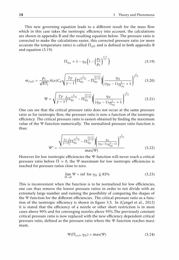
One can see that the critical pressure ratio does not occur at the same pressureratio as for isentropic flow, the pressure ratio is now a function of the isentropicefficiency. The critical pressure ratio is easiest obtained by finding the maximumvalue of the Ψ -function numerically. The normalized pressure ratio function isthus:
Ψ ∗ =
√2γγ−1
(Π
2(γ−1)ηN −Π
(γ+1)(γ−1)ηN
) ηN(ηN−1) 1
ΠηN+1
γγ−1
max(Ψ )(3.22)
However for low isentropic efficiencies the Ψ -function will never reach a criticalpressure ratio before Π ≈ 0, the Ψ -maximum for low isentropic efficiencies isreached for pressure ratios close to zero.
limΠ→0
Ψ = inf for ηN / 85% (3.23)
This is inconvenient when the function is to be normalized for low efficiencies,one can thus remove the lowest pressure ratios in order to not divide with anextremely large number and ruining the possibility of comparing the shapes ofthe Ψ -function for the different efficiencies. The critical pressure ratio as a func-tion of the isentropic efficiency is shown in figure 3.5. In (Çengel et al., 2012)it is stated that the efficiency of a nozzle or other short restriction is in mostcases above 90% and for converging nozzles above 95%.The previously constantcritical pressure ratio is now replaced with the new efficiency dependent criticalpressure ratio, defined as the pressure ratio where the Ψ -function reaches maxi-mum.
Ψ (Πcrit , ηN ) = max(Ψ ) (3.24)
3.2 Steady Non-Isentropic Compressible Flow 19
Ψ (Π) =
1 if 0 < Π ≤ Πcrit
Ψ ∗(Π) if Πcrit < Π ≤ Πlin
Ψ ∗(Π) Π−1Πlin−1 if Πlin < Π ≤ 1
(3.25)
0.2 0.3 0.4 0.5 0.6 0.7 0.8 0.9 1 1.1
Π
0
0.2
0.4
0.6
0.8
1
Ψ*
Normalized Ψ*(Π ) - function for different isentropic efficiencies
ηN
=100%
ηN
=95%
ηN
=90%
ηN
=85%
ηN
=80%
Figure 3.4: Here the Ψ -function for various isentropical efficiencies over anozzle can be seen with both linearized area for pressure ratios over 0.99.Also for pressure ratios below the critical ratio the function are set to one.

20 3 Theory and Phenomena
0.85 0.9 0.95 1
Isentropic efficiency ηN [-]
0.3
0.35
0.4
0.45
0.5
0.55
Critical pre
ssure
ratio Π
[-]
Figure 3.5: Here the critical pressure ratio is shown as a function of theisentropic efficiency, worth noting is that for efficiencies below 85% thereis no critical pressure ratio since the extended Ψ -function does not have amaximum value here as stated in equation (3.23)
3.3 Pulsating Pressure Ratio
The use of a mean pressure ratio when calculating the momentarily mass flowcan be one factor that effects the deviating shape of the Ψ -function. Since theΨ -function is non-linear the assumption that the average pressure ratio can beused to calculate the mean Ψ -function value is incorrect but might be sufficient.The assumption is explained in figure 3.6.
Ψ =
Ψ (mean(Π)) assumption which is used.mean(Ψ (Π)) correct way.
(3.26)
For pulsating flows this assumption would in theory distort the Ψ -functionin the same way as is shown in (Andersson, 2005) where the real Ψ -values is abit under the theoretical Ψ -function. However if the intake pulsations is largeenough to explain the deviation or if it is the isentropic efficiency which causesthis effect needs to be investigated further.

3.4 Unsteady Isentropic Compressible Flow 21
0.6 0.7 0.8 0.9 1
Figure 3.6: If the pressure ratio is pulsating between the two outer dashedlines and the mean pressure ratio is the dotted line, using the mean pressureratio to calculate the Ψ -value one gets the upper dot on the Ψ -function line.The correct way to calculate the average Ψ -value is for every time step cal-culate the Ψ -function value and then take the average of these. The lowerdot is thus obtained, the difference is shown in equation (3.26)
3.4 Unsteady Isentropic Compressible Flow
Using Newton’s second law of motion on a fluid particle in an unsteady com-pressible flow, and neglecting the gravity, which often can be done assumingsmall height differences in the flow, one gets the 1-D linear momentum equation,derivation shown in appendix C.
1ρ
∂p
∂x+ v
∂v∂x
+∂v∂t
= 0 (3.27)

22 3 Theory and Phenomena
Assuming isentropic processes in the flow the isentropical relation between den-sity and pressure, can be used to substitute the density in equation (3.27) with astagnation/inlet density and pressure.
ρ
ρ0=
( pp0
) 1γ
(3.28)
1ρ0
(p0
p
) 1γ ∂p
∂x+ v
∂v∂x
+∂v∂t
= 0 (3.29)
Applying the equation to a restriction in a pipe, the assumption that the variablesonly change with the length of the pipe but is the same for every cross section areais to be made. The flow is thus uniform, and have only one dimension, hence theabove equation (3.29) applies. The equation also assumes isentropic flow, this ismotivated by the small effect the isentropic efficiency have when pressure ratiois close to one, where this model is intended for use. Further integrating theequation from the start of the pipe x0 where the pressure is p0 to xt and pressurept , t, indicating the throat of the valve. Also assuming that the inlet velocity isnegligible v0 ≈ 0 the integration becomes:
p1γ
0ρ0
xt∫x0
1
p1γ
dp +v2t
2+
xt∫x0
∂v∂tdx = 0 (3.30)
Further simplifications and assumptions of the equation above, shown in ap-pendix C, gives an unsteady compressible mass flow equation where an extradynamic term is added to the previous steady equation. Similar assumptionsand calculations as in appendix C are made in (Kiwan et al., 2016)
A2ef f C
2d
p20
T0R
2γγ − 1
(Π
2γ −Π
γ+1γ
)= m2 + AdynA
2ef f C
2d
2p0
T0RΠ
2γ∂m∂t
(3.31)
In order to deal with the possibility of reversing mass flows some comparisonsare to be made in order to determine in which direction the pressure ratio forcesthe flow. The flow does not necessary flow from high pressure to low pressuresince the inertia of the flow can force flow from low to high pressure.
po =
p1 if p1 ≥ p2
p2 if p1 < p2(3.32)
To =
T1 if p1 ≥ p2
T2 if p1 < p2(3.33)
Π =
p2p1
if p1 ≥ p2p1p2
if p1 < p2(3.34)

3.4 Unsteady Isentropic Compressible Flow 23
The mass flow direction is of interest and needs to be determined, the equa-tion only states the magnitude. To ensure this effect is described the steady partof the equation have to change sign when the flow is driven from p2 to p1 if thepositive flow is defined from p1 to p2. The mass flow square are to be dividedinto two parts, one with absolute sign, to prevent the square from removing thesign dependency.
sign(p1 − p2)A2ef f C
2d
p20
T0R
2γγ − 1
(Π
2γ −Π
γ+1γ
)= m|m| + AdynA2
ef f C2d
2p0
T0RΠ
2γ∂m∂t
(3.35)


4Approach
In this chapter the approach used when taking measurements and how the modelparameters are calculated is presented. The valves which the previous presentedmodels are intended for are the ones in a combustion engine, where the dynamicone is intended for low pressure ratios such as when a long route egr system isused. The system is presented in figure 4.1.
Throttle
Wastegate
Long-Route EGR valve
Oxygen sensor
Mass flow sensor
Air filter
Turbine
Compressor
Intercooler
Long-route EGR system
Follwing exhaust system
Intake manifold Exhaust manifold
Cylinders
Figure 4.1: Here a schematic air path system is shown for a turbocharged en-gine with long route egr system, long route egr is shown within the dashedline. The oxygen sensor shown is just an example on how the flow past thelong route egr can be estimated.
25
26 4 Approach
4.1 Steady Compressible Flow
In this section the approach and how the measurements are taken for the steadynon-isentropic model is presented.
4.1.1 Approach
To validate the theoretical calculations and formulas in the two sections regard-ing steady compressible flow in the theory chapter, the approach and some thoughtsare described in the following section. The goal is to validate the Ψ -functionagainst real measured data not only theoretically , however the Ψ -function is nota measurable state, some calculations is needed. To start of the isentropical effi-ciency needs to be determined. This is done by doing measurements on a throttleduring steady flow and using the following formula, where all the states are easilymeasured in the part rightmost, except T2a. The temperature at the throat of thevalve cant be measured since it is a very local temperature and after the valve thegenerated speed causes turbulence and temperature rise. The temperature needsto be determined analytical using ANSYS or the efficiency is to be approximatedplotting the Ψ -function and using lsqcurvefit to chose the isentropic efficiencythat minimizes the error in the model.
ηN =V 2
2a
V 22s
=T1 − T2a
T1 − T2s=
T1 − T2a
T1 − T1
(p2p1
) (γ−1)γ
(4.1)
To determine if the efficiency can be seen as a constant, or if it is pressure ratiodependent, or perhaps throttle angle dependent, measurements need to be done.This is done different pressure ratios, and throttle angles, only then the depen-dency can be determined. The isentropic efficiency can also be input temperaturedependent (T1), however since it is hard to generate a wide range of input tem-peratures this will only be investigated for the temperatures which is naturallyobtained when making the tests for different pressure ratios, and angles.
The mass flow function is as stated before, here with the addition of an angle,and pressure ratio dependent Cd .
m =p1√RT1
A(α)Cd(α,Π)Ψ (Π, ηN ) (4.2)
The angle dependant Cd part can be assumed to be absorbed by the A(α) whichcombined is called Aef f (α).
m =p1√RT1
Aef f (α)Cd(Π)Ψ (Π, ηN ) (4.3)
First of assuming that the isentropic efficiency is high enough so that there willbe a critical pressure ratio in the Ψ -function. For pressure ratios below the criti-cal pressure ratio the Ψ -function will thus be one, as defined before. Setting thethrottle at a fixed position will make the effective area Aef f a constant. Making

4.1 Steady Compressible Flow 27
sweeps in the pressure ratio for fixed throttle angle, and normalizing with the val-ues obtained for pressure ratios below the critical pressure ratio, C∗d(Π)Ψ ∗(Π, ηN )can be extracted.
p1√RT1
Aef f (α)Cd(Π)Ψ (Π, ηN )p1√RT1
Aef f (α) Cd(Π < Πcrit)Ψ (Π < Πcrit , ηN )︸ ︷︷ ︸Assumed one for the lowest pressure ratios
=m
m(Π < Πcrit)= C∗d(Π)Ψ ∗(Π, ηN )
(4.4)In short terms, the mass flow is measured and divided with the mean value of themaximum mass flows, which occurs below the critical pressure ratio, thus the nor-malized C∗d(Π)Ψ ∗(Π, ηN )-function is obtained. The theoretical Ψ -function cannow be compared with C∗d(Π)Ψ ∗(Π, ηN ) in order to determine if Cd(Π) can beneglected, this is done both for isentropic Ψ -function (ηN = 100%), and for thenon-isentropic Ψ -function which uses isentropic efficiency. This to determineif the Ψ -function taking the efficiency into account can explain the deviationsbetween the isentropic Ψ -function and C∗d(Π)Ψ ∗(Π), shown in for example (An-dersson, 2005) where the Cd(Π) can not be neglected. When the Ψ -function havebeen calculated the effective area function can easily be determined, using someassumed polynomial expression and lsqcurvefit to decide the coefficients. Thepolynomial which is used are proposed in (Eriksson and Nielsen, 2014) and is de-scribed in equation (4.5) where ai are the coefficients which are to be determined.
Aef f = a0 + a1α + a2α2 (4.5)
4.1.2 Measurements
Since the derived equations assume that the flow is steady, no change with time,and in the intake manifold of an engine there is plenty of pulsations coming fromthe intake valves the measurements are thus preferable made in a flow benchwhere there no pulsations are generated. This to ensure that the phenomenawhich causes the deviation in the theoretical Ψ -function from the measurementsin (Andersson, 2005) is not caused by the pulsations. Signals to be measured aretemperature and pressure, before and after the throttle, the mass flow past thethrottle, and throttle angle. This is done for various fixed throttle angles and forevery angle a wide range of pressure ratios. The flow test is carried out at Volvoin their flow bench and a picture of the setup is shown in figure 4.2.
When deciding the Aef f (α)-function the measurements are done for variousthrottle angles from the idle opening, to fully open, and for some various pres-sure ratios that the flow bench can mange to produce when throttle is fully open.Same signals are to be collected in this case.

28 4 Approach
Figure 4.2: Here a standard Volvo throttle housing is mounted with sensorsin the flow bench at VCC, a loss free cone is used to reduce inlet turbulence.
4.2 Unsteady Compressible Flow
In this section the theoretical approach by which the dynamic compressible massflow model parameters can be calculated is presented. Suggestions on how themeasurements are to be conducted is also described.
4.2.1 Approach
The approach in which the dynamic compressible flow function is determined ispartly the same as for the static equation. The effective area Aef f and isentropicefficiency is determined just as for the static function. However the efficiencymight be neglected due to the fact that the Ψ -function for pressure ratios close

4.2 Unsteady Compressible Flow 29
to one is almost the same regardless of the efficiency, and the dynamic functionmain use is for pressure ratios close to one where the pulsating effects are largeand one needs to account for backflow. If one needs a model for a valve whichboth should work for low pressure ratios where the efficiency needs to be takeninto account, and for pressure ratios close to one where the dynamic effects cantbe ignored, the previous derived compressible flow equation with regard to ef-ficiency can replace the static part of the dynamic flow equations otherwise theoriginal Ψ -function can be used.
The similarity between the unsteady compressible flow equation and a firstorder system is striking, the difference is the square of the mass flow term. Thesquare term can however easily be linearized around m0, here the static term isreplaced with ζ and the dynamic term with φ.
ζ = m2 + Adynφdmdt
(4.6)
Variable change:
∆m = m − m0 (4.7)
And for mass flows close to m0:
m2 ≈ m20 + 2m0∆m (4.8)
ζ = m20 + 2m0∆m + Adynφ
d∆mdt
(4.9)
Laplace transforming gives the first order system:
ζ − m20
2m0 + sAdynφ= ∆m (4.10)
The time constant is thus as follows and the Adyn can be determined by makingsteps in mass flow rate for different plate angles and at different linearized massflow magnitudes.
Adynφ
2m0= τ (4.11)
Adyn =2m0τφ
(4.12)
To determine which variables that affect the dynamic area function further in-vestigations on how a number of parameters, such as mass flow, pressure ratio,temperature and so on, affect the measured values for Adyn. This in order todetermine if Adyn can be considered a constant or is dependant on some otherparameter and a function can be determined.
30 4 Approach
4.2.2 Measurements
The data that is to be collected needs to be highly resolved in order to capturethe pulsations coming from the filling and emptying of the cylinders. Whenevaluating the dynamic model on the throttle side a regular mass flow metercan be used, as long as it samples fast enough. However for the long route egrvalve which the dynamic model is intended to be used for the mass flow can notbe measured directly. One way to estimate the mass flow over the long routeegr valve is to measure the oxygen level on the intake side of the engine afterthe mixing point of the fresh air and exhaust gases, see figure 4.1. Defining thepercentage of oxygen in a gas as:
O2% =mOmtot
(4.13)
Assuming that the percentage of oxygen in both fresh air and exhaust gas isknown the precentage of oxygen after the mixing point can be described as:
O2% =O2%air mair + O2%exhaustmEGR
mair + mEGR(4.14)
Thus the mass flow over the egr valve can be described using a mass flow sensorand an oxygen sensor.
mEGR = mairO2%air − O2%
O2% − O2%EGR(4.15)
This approach is however problematic since oxygen sensors is not fast enough tomeasure the pulsations which occurs twice per engine revolution in the intakemanifold. A high resolved air mass flow sensor can be used instead and the dy-namic model thus have to be evaluated on the throttle instead of the egr valve.

5Results
Here the results of this master’s thesis is presented. For example the measureddata both from an engine and a flow bench against standard and extended modelis shown. The simulation results from both ansys and simulink is also pre-sented.
5.1 Fixed Throttle Position
In order to eliminate the area dependant factor when calculating the Ψ -functionmeasurements are made for fixed throttle positions, thus the effective area canbe seen as a constant and eliminated. Measurements are made for three differentthrottle angles, however for the throttle angle at 5 degrees only a very small rangeof pressure ratios was possible to archive due to the limitations in the enginesworking range. These measurements are made on an engine thus the intake pul-sations is present. One can clearly see the deviation between the measured andtheoretical values in figure 5.1, just as in (Andersson, 2005).
31

32 5 Results
0.2 0.3 0.4 0.5 0.6 0.7 0.8 0.9 1 1.1
Π
0
0.2
0.4
0.6
0.8
1
Ψ*
Normalized Ψ*(Π ) - function
Ψ -function
5 deg throttle
10 deg throttle
20 deg throttle
Figure 5.1: The Simulation model used to calculate the normalized Ψ -valuesfor different pressure ratios with the effect of intake manifold pulsations.
5.2 Normal and Extended Ψ -function
Using data where the pressure before and after the throttle, temperature beforethe throttle, mass flow past the throttle, and throttle angle are measured duringstationary conditions makes it possible to evaluate the Ψ -function. Furthermorethe isentropic flow equation is used and compared with the non isentropic flowequation in order to determine if an improvement is achieved.
5.2.1 Engine Measurements
These measurements are made on an engine, thus the pulsations are present, andthe deviation in the Ψ -function can not definitely be explained by the efficiency,it can also be the pulsations effecting the flow. In figure 5.2 the isentropic flowequation is used, and in figure 5.3 the non-isentropic flow equation is used andthe optimal efficiency is determined using lsqcurvefit. In order to eliminate theeffective area term from the model the effective area is modeled and then substi-tuted in order to obtain the Ψ -function. In figure 5.4 the difference between thefit of the normal and extended Ψ -function is shown along with the calculatedΨ -values from the data.

5.2 Normal and Extended Ψ -function 33
0 5 10 15 20 25 30 35 40
alpha [deg]
0
0.5
1
1.5
2
2.5
3
Effective a
rea [m
3]
×10-4 Normal Ψ - function
Measured
Modelled
(a) Measured and modelled effective areawhen the isentropic Ψ -function is used.
0.2 0.3 0.4 0.5 0.6 0.7 0.8 0.9
Π [-]
0
1
2
3
4
5
6
7
8
9
10
rela
tive e
rror
[%]
Normal Ψ - function
(b) Relative effective area error when theisentropic Ψ -function is used.
Figure 5.2: Effective area model when the isentropic Ψ -function is used. Themean relative error is in this case 2.89%
0 5 10 15 20 25 30 35 40
alpha [deg]
0
0.5
1
1.5
2
2.5
3
Effective a
rea [m
3]
×10-4 Extended Ψ - function
Measured
Modelled
(a) Measured and modelled effective areawhen the non-isentropic Ψ -function isused.
0.2 0.3 0.4 0.5 0.6 0.7 0.8 0.9
Π [-]
0
1
2
3
4
5
6
7
8
9
10
rela
tive e
rror
[%]
Extended Ψ - function
(b) Relative effective area error when thenon-isentropic Ψ -function is used.
Figure 5.3: Effective area model when the non-isentropic Ψ -function is used,the efficiency which minimizes the relative error is 96.5%. The mean relativeerror is in this case 2.69% which is a 7% decrease in relative error.

34 5 Results
0.2 0.3 0.4 0.5 0.6 0.7 0.8 0.9 1 1.1
Π
0
0.2
0.4
0.6
0.8
1
Ψ*
Normalized Ψ*(Π ) - function and calculated Ψ - data
Ψ Data
ηN
=96.5%
ηN
=100%
Figure 5.4: The normalized Ψ -data points is here shown together with boththe standard 100% isentropic efficiency equation and with 96.5% efficiency,which is obtained using lsqcurvefit.
0.2 0.3 0.4 0.5 0.6 0.7 0.8 0.9 1
Π [-]
0
2
4
6
8
10
12
rela
tive e
rror
[%]
Reltive error for the standard Ψ - function
(a) Relative error when the standard Ψ -function is used, the mean relative erroris here 4.16 %.
0.2 0.3 0.4 0.5 0.6 0.7 0.8 0.9 1
Π [-]
0
2
4
6
8
10
12
rela
tive e
rror
[%]
Reltive error for the extended Ψ - function
(b) Relative error when the extended Ψ -function is used, the mean relative error ishere 2.92 %.
Figure 5.5: Pressure ratios above 0.95 is removed due to the linear region inthe model which have a big relative error and thus only makes it harder tocompare the improvement in the model. The total improvement in relativeerror is over 30% for the extended model.

5.2 Normal and Extended Ψ -function 35
5.2.2 Flow Bench Measurements
These measurements are made with a flow bench, thus pulsations are not present,and the deviation in the Ψ -function can with these results with certainty excludethe pulsations as the deviating factor.
0.2 0.3 0.4 0.5 0.6 0.7 0.8 0.9 1 1.1
Π
0
0.2
0.4
0.6
0.8
1
Ψ*
Normalized Ψ*(Π ) - function with measured data
Theory
α=2
α=5
α=10
α=15
α=20
α=30
Figure 5.6: The isentropic normalized Ψ -function is here shown togetherwith the data collected in the flow bench for various throttle angles. Onecan see that the efficiency is varying with the throttle angle and the figureindices that a smaller opening have higher efficiency.
The data collected in the flow bench is used to calculate the efficiency for everyfixed area opening using lsqcurvefit, the result is shown in figure 5.7. The errorbetween the measured values and the non-isentropic Ψ -function when the esti-mated efficiency is used is very small, more details of the relative error is shownin figure 5.8. Using a non-pressure dependant efficiency can be motivated by thesmall differences in relative error over the Π-range. Also the area dependant ef-fect on the isentropic efficiency can perhaps be neglected, the only big deviationin efficiency is for a throttle opening of 5 degrees.
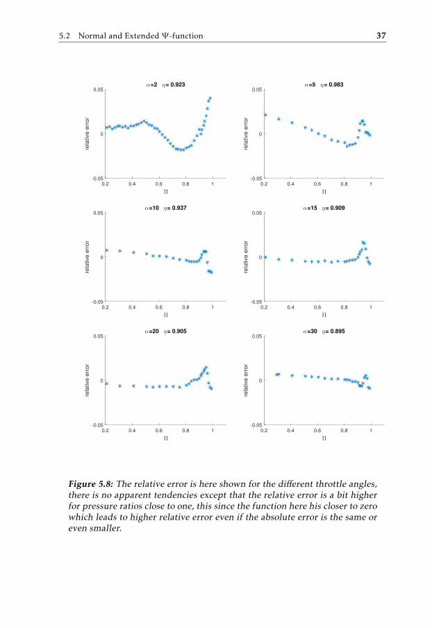
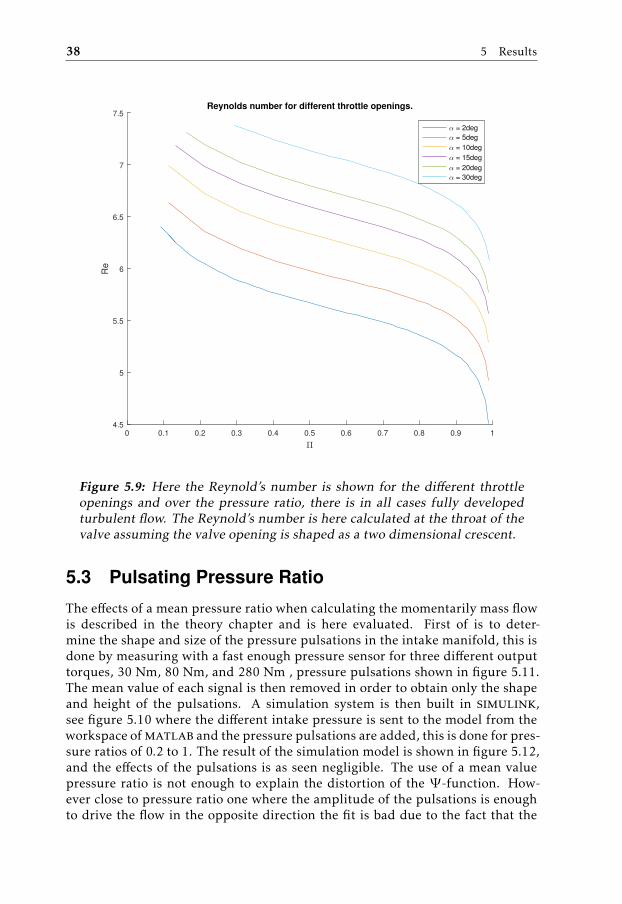
The Reynold’s number can be calculated using equation (5.1). The resultswhen calculating the Reynold’s number can be seen in figure 5.9. For a fluid flow-ing in circular pipe the critical Reynold’s number where the flow is shifting fromlaminar to turbulent is said to be around 2000 < Re < 4000 and if there is someobstacle or a rough surface in the tube turbulent flow will evolve much faster,
36 5 Results
0.2 0.4 0.6 0.8 1
Π
0
0.2
0.4
0.6
0.8
1
Ψ*
α=2 η= 0.923
0.2 0.4 0.6 0.8 1
Π
0
0.2
0.4
0.6
0.8
1
Ψ*
α=5 η= 0.983
0.2 0.4 0.6 0.8 1
Π
0
0.2
0.4
0.6
0.8
1
Ψ*
α=10 η= 0.937
0.2 0.4 0.6 0.8 1
Π
0
0.2
0.4
0.6
0.8
1
Ψ*
α=15 η= 0.909
0.2 0.4 0.6 0.8 1
Π
0
0.2
0.4
0.6
0.8
1
Ψ*
α=20 η= 0.905
0.2 0.4 0.6 0.8 1
Π
0
0.2
0.4
0.6
0.8
1
Ψ*
α=30 η= 0.895
Figure 5.7: The isentropic Ψ -function is the dashed line, the measured val-ues from the flow bench is the blue line, and the red line is the non-isentropicΨ -function when the efficiency is estimated using lsqcurvefit.
(Karl Storck, 2012). The flow is according to the calculated Reynold’s numberfully developed turbulent in all the cases.
Re =LUv
=dh
mρA
v=
4mOρ
v=
4mRTOp2
v(5.1)
5.2 Normal and Extended Ψ -function 37
0.2 0.4 0.6 0.8 1
Π
-0.05
0
0.05re
lative e
rror
α=2 η= 0.923
0.2 0.4 0.6 0.8 1
Π
-0.05
0
0.05
rela
tive e
rror
α=5 η= 0.983
0.2 0.4 0.6 0.8 1
Π
-0.05
0
0.05
rela
tive e
rror
α=10 η= 0.937
0.2 0.4 0.6 0.8 1
Π
-0.05
0
0.05
rela
tive e
rror
α=15 η= 0.909
0.2 0.4 0.6 0.8 1
Π
-0.05
0
0.05
rela
tive e
rror
α=20 η= 0.905
0.2 0.4 0.6 0.8 1
Π
-0.05
0
0.05
rela
tive e
rror
α=30 η= 0.895
Figure 5.8: The relative error is here shown for the different throttle angles,there is no apparent tendencies except that the relative error is a bit higherfor pressure ratios close to one, this since the function here his closer to zerowhich leads to higher relative error even if the absolute error is the same oreven smaller.
38 5 Results
0 0.1 0.2 0.3 0.4 0.5 0.6 0.7 0.8 0.9 1
Π
4.5
5
5.5
6
6.5
7
7.5R
eReynolds number for different throttle openings.
α = 2deg
α = 5deg
α = 10deg
α = 15deg
α = 20deg
α = 30deg
Figure 5.9: Here the Reynold’s number is shown for the different throttleopenings and over the pressure ratio, there is in all cases fully developedturbulent flow. The Reynold’s number is here calculated at the throat of thevalve assuming the valve opening is shaped as a two dimensional crescent.
5.3 Pulsating Pressure Ratio
The effects of a mean pressure ratio when calculating the momentarily mass flowis described in the theory chapter and is here evaluated. First of is to deter-mine the shape and size of the pressure pulsations in the intake manifold, this isdone by measuring with a fast enough pressure sensor for three different outputtorques, 30 Nm, 80 Nm, and 280 Nm , pressure pulsations shown in figure 5.11.The mean value of each signal is then removed in order to obtain only the shapeand height of the pulsations. A simulation system is then built in simulink,see figure 5.10 where the different intake pressure is sent to the model from theworkspace ofmatlab and the pressure pulsations are added, this is done for pres-sure ratios of 0.2 to 1. The result of the simulation model is shown in figure 5.12,and the effects of the pulsations is as seen negligible. The use of a mean valuepressure ratio is not enough to explain the distortion of the Ψ -function. How-ever close to pressure ratio one where the amplitude of the pulsations is enoughto drive the flow in the opposite direction the fit is bad due to the fact that the

5.3 Pulsating Pressure Ratio 39
used model cant handle back flow.
Figure 5.10: The Simulation model used to calculate the normalized Ψ -values for different pressure ratios with the effect of intake manifold pul-sations.

40 5 Results
-400 -300 -200 -100 0 100 200 300 400
Crank Angle [deg]
3.5
4
4.5
5
Inta
ke
Pre
ssu
re [
Pa
]
×104
-400 -300 -200 -100 0 100 200 300 400
Crank Angle [deg]
7
7.5
8
8.5
9
Inta
ke
Pre
ssu
re [
Pa
]
×104
-400 -300 -200 -100 0 100 200 300 400
Crank Angle [deg]
1.55
1.6
1.65
1.7
1.75
Inta
ke
Pre
ssu
re [
Pa
]
×105
Figure 5.11: Intake manifold pressure pulsations for three different engineloads, first is 30 Nm where the amplitude is 10 kPa, second 80 Nm where theamplitude is 14 kPa, and last 280 Nm where the amplitude is 16 kPa. Thevertical lines shows where the intake valve closes for each cylinder.

5.3 Pulsating Pressure Ratio 41
0.2 0.3 0.4 0.5 0.6 0.7 0.8 0.9 1
Π
0
0.2
0.4
0.6
0.8
1
Ψ*
Normalized Ψ*(Π ) - function with simulated data
Theoretical Ψ -function
Torque 30Nm
Torque 80Nm
Torque 280Nm
Figure 5.12: The theoretical Ψ -function along with the calculated Ψ -function for the three different engine load pressure pulsations. The devi-ation from the theory close to pressure ratio one is due to the fact that thepulsations causes pressure ratio to go above one which leads to back flowwhich is not taken into account in the model. The deviation from theorydue too pulsations is to small and can not explain the quite large deviationshown in (Andersson, 2005)
42 5 Results
5.4 Throttle Valve ANSYS Analysis
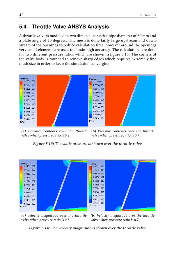
A throttle valve is modeled in two dimensions with a pipe diameter of 60 mm anda plate angle of 20 degrees. The mesh is done fairly large upstream and down-stream of the openings to reduce calculation time, however around the openingsvery small elements are used to obtain high accuracy. The calculations are donefor two different pressure ratios which are shown in figure 5.13. The corners ofthe valve body is rounded to remove sharp edges which requires extremely finemesh size in order to keep the simulation converging.
(a) Pressure contours over the throttlevalve when pressure ratio is 0.8.
(b) Pressure contours over the throttlevalve when pressure ratio is 0.7.
Figure 5.13: The static pressure is shown over the throttle valve.
(a) velocity magnitude over the throttlevalve when pressure ratio is 0.8.
(b) Velocity magnitude over the throttlevalve when pressure ratio is 0.7.
Figure 5.14: The velocity magnitude is shown over the throttle valve.
5.4 Throttle Valve ANSYS Analysis 43
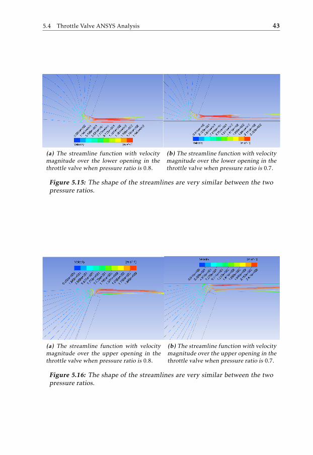
(a) The streamline function with velocitymagnitude over the lower opening in thethrottle valve when pressure ratio is 0.8.
(b) The streamline function with velocitymagnitude over the lower opening in thethrottle valve when pressure ratio is 0.7.
Figure 5.15: The shape of the streamlines are very similar between the twopressure ratios.
(a) The streamline function with velocitymagnitude over the upper opening in thethrottle valve when pressure ratio is 0.8.
(b) The streamline function with velocitymagnitude over the upper opening in thethrottle valve when pressure ratio is 0.7.
Figure 5.16: The shape of the streamlines are very similar between the twopressure ratios.
44 5 Results
10 20 30 40 50 60 70
entropy [J/K]
2.65
2.7
2.75
2.8
2.85
2.9
2.95
enth
alp
y [J/K
g]
×105 h-s diagram for the lower stream lines
(a) The throttling process for the loweropening in the valve, this for a pressure ra-tio of 0.7.
10 20 30 40 50 60 70
entropy [J/K]
2.65
2.7
2.75
2.8
2.85
2.9
2.95
enth
alp
y [J/K
g]
×105 h-s diagram for the upper stream lines
(b) The throttling process for the upperopening in the valve, this for a pressure ra-tio of 0.7.
15 20 25 30 35 40 45 50 55
entropy [J/K]
2.76
2.78
2.8
2.82
2.84
2.86
2.88
2.9
2.92
2.94
2.96
enth
alp
y [J/K
g]
×105 h-s diagram for the lower stream lines
(c) The throttling process for the loweropening in the valve, this for a pressure ra-tio of 0.8.
15 20 25 30 35 40 45 50 55
entropy [J/K]
2.76
2.78
2.8
2.82
2.84
2.86
2.88
2.9
2.92
2.94
2.96
enth
alp
y [J/K
g]
×105 h-s diagram for the upper stream lines
(d) The throttling process for the upperopening in the valve, this for a pressureratio of 0.8. Here the flow simulated doesnot seem to be fully developed.
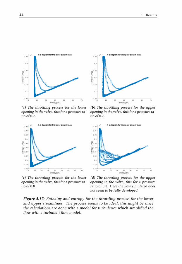
Figure 5.17: Enthalpy and entropy for the throttling process for the lowerand upper streamlines. The process seems to be ideal, this might be sincethe calculations are done with a model for turbulence which simplified theflow with a turbulent flow model.

5.5 Dynamic Compressible Flow 45
5.5 Dynamic Compressible Flow
A regular mas flow meter measures the air mass flow through the pipe with thehelp of a platinum wire. A current is sent through the wire, the more mass flowthe more the wire will be cooled which leads to lower resistance and the otherway around for lower mass flows. The mass flow can thus be measured after thesensor has been calibrated towards a known flow in a flow bench. The dynamicmeasurements is carried out in the engine-lab at ISY with one millisecond sam-pling of the new mass flow sensor which uses a thin film to measure the varyingresistance instead of a platinum wire as before. The film reacts much faster tochanges than the wire due to the greater area to mass ratio which cools or heatsthe film faster then the wire. The raw measured signals for the mass flow canbe seen in figure 5.18 and the related intake manifold pressure in figure 5.19.The measured boost pressure (pressure before the throttle) can be consideredconstant since it only oscillates with the resolution of the digital pressure sensor,0.08 kPa.
0 2 4 6 8 10
Time [s]
1.5
2
2.5
3
Hz [1/s
]
Mean Π = 0.3
0 2 4 6 8 10
Time [s]
2.8
2.9
3
3.1
3.2
3.3
Hz [1/s
]
Mean Π = 0.5
0 2 4 6 8 10
Time [s]
1.5
2
2.5
3
3.5
4
Hz [1/s
]
Mean Π = 0.64
Raw measured MAF-sensor signal
0 2 4 6 8 10
Time [s]
2
2.5
3
3.5
4
Hz [1/s
]
Mean Π = 0.79
Figure 5.18: The measured air mass flow signal for four different loads andthus pressure ratios, the frequency needs to be converted to mass flow withthe help of the calibration line for this particular sensor. The sudden spikesin the data is probably measurement errors due to bad connections in thewiring.

46 5 Results
0 2 4 6 8 10
Time [s]
29
29.5
30
30.5
31
31.5
Pre
ssure
[kP
a]
Mean Π = 0.3
0 2 4 6 8 10
Time [s]
49
50
51
52
53
Pre
ssure
[kP
a]
Mean Π = 0.5
0 2 4 6 8 10
Time [s]
63
64
65
66
67
68
Pre
ssure
[kP
a]
Mean Π = 0.64
Raw measured intake manifold pressure
0 2 4 6 8 10
Time [s]
77
78
79
80
81
82
Pre
ssure
[kP
a]
Mean Π = 0.79
Figure 5.19: Here the intake manifold pressure for the four different casescan be seen, in the case of pressure ratio 0.5 some load change happens atthe end. Here the data is cleaner and needs no pre-filtering as in the massflow case.
The data from the mass flow sensor is pre-filtered by replacing the values thatdeviate too much from the previous values in the time series with the previousvalue, this removes the sudden spikes that can be seen in the raw air mass flowsensor signal. Furthermore both intake manifold pressure signal and the massflow signal is filtered with a butterworth filter and the filtfilt function in mat-lab, which is a no phase shifting filter. After filtering the frequency from themass flow sensor, the frequency is converted to actual mass flow air in grams persecond using the given calibration line supplied by VCC, shown in figure 5.20.The filtered and the raw signal for the mass flow can be seen in figure 5.21 whichis zoomed so it is possible to see the difference, where the zoom position is ran-domly chosen. The same case for the pressure in the intake manifold can be seenin figure 5.22.
Furthermore the pressure signal is applied to the static non-isentropic com-pressible flow equation with an isentropic efficiency of 95%, the effective areafunction is calculated from data taken in the flow bench see figure 5.23. The re-sulting modelled mass flow is then compared to the measured and the result canbe seen in figure 5.24, the mean flow was corrected by a very small portion just

5.5 Dynamic Compressible Flow 47
1 2 3 4 5 6 7 8 9 10
Frequency [Hz]
-50
0
50
100
150
200
250
300
350
400M
ass F
low
[g
/s]
Calibration line converting [Hz] to [g/s]
Figure 5.20: The calibration line converting the measured frequency to airmass flow in grams per second, this particular mass flow meter can evenhandle back flows thus presenting a negative value.
so that the mean flow of both signals is at the same level which makes it easierto compare. The phase difference between the model and the measured values isdue to the distance from measured pressure to measured mass flow which causesa time delay. However in order to implement the dynamic flow equation to pre-dict the instantaneous flow past the throttle the measurements should have beendone without any turbo or intercooler which disturbs the flow. A spectral analysisis made and the result is shown in figure 5.25

48 5 Results
4.6 4.62 4.64 4.66 4.68 4.7 4.72
Time [s]
3.15
3.2
3.25
Mass flo
w [g/s
]
Mean Π = 0.3
2.95 3 3.05 3.1 3.15
Time [s]
5.6
5.65
5.7
5.75
5.8
5.85
Mass flo
w [g/s
]
Mean Π = 0.5
5.06 5.08 5.1 5.12 5.14 5.16 5.18
Time [s]
7.4
7.5
7.6
7.7
7.8
Mass flo
w [g/s
]
Mean Π = 0.64
Filtered measured mass flow air.
3.46 3.48 3.5 3.52 3.54 3.56 3.58
Time [s]
9.2
9.4
9.6
9.8
Mass flo
w [g/s
]
Mean Π = 0.79
Figure 5.21: Here the filtered mass flow signal can be seen together withthe raw signal, the blue line is the filtered signal and the red is the raw data.After pre-filtering and filtering the data is converted from frequency to massflow.
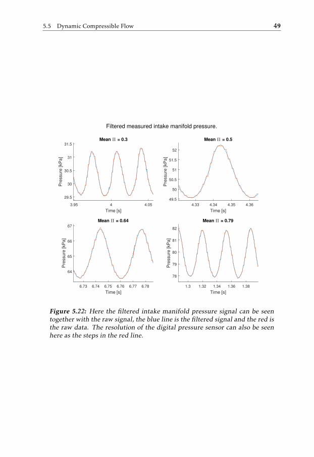
5.5 Dynamic Compressible Flow 49
3.95 4 4.05
Time [s]
29.5
30
30.5
31
31.5
Pre
ssure
[kP
a]
Mean Π = 0.3
4.33 4.34 4.35 4.36
Time [s]
49.5
50
50.5
51
51.5
52
Pre
ssure
[kP
a]
Mean Π = 0.5
6.73 6.74 6.75 6.76 6.77 6.78
Time [s]
64
65
66
67
Pre
ssure
[kP
a]
Mean Π = 0.64
Filtered measured intake manifold pressure.
1.3 1.32 1.34 1.36 1.38
Time [s]
78
79
80
81
82
Pre
ssure
[kP
a]
Mean Π = 0.79
Figure 5.22: Here the filtered intake manifold pressure signal can be seentogether with the raw signal, the blue line is the filtered signal and the red isthe raw data. The resolution of the digital pressure sensor can also be seenhere as the steps in the red line.

50 5 Results
0 5 10 15 20 25 30 35 40
alpha [α]
0
0.5
1
1.5
2
2.5
3
3.5
4
Eff
ectiv a
rea
[m
2]
×10-4 Effectiv area measured in flow bench
Figure 5.23: Here is the measured effective area shown, this line is usedwhen calculating the flow from the pulsating intake manifold pressure.

5.5 Dynamic Compressible Flow 51
3.7 3.8 3.9 4
Time [s]
3.15
3.2
3.25
Ma
ss f
low
[g
/s]
Mean Π = 0.3
3.1 3.15 3.2
Time [s]
5.65
5.7
5.75
5.8
5.85
Ma
ss f
low
[g
/s]
Mean Π = 0.5
7.3 7.35 7.4 7.45
Time [s]
7.4
7.5
7.6
7.7
7.8
Ma
ss f
low
[g
/s]
Mean Π = 0.64
Filtered measured mass flow air plotted against modelled massflow.
3.7 3.75 3.8 3.85
Time [s]
9.2
9.4
9.6
9.8
Ma
ss f
low
[g
/s]
Mean Π = 0.79
Figure 5.24: Here the measured mass flow signal, blue line, together withthe modelled mass flow, red line, is shown. When pressure ratio is belowthe critical pressure ratio the model indicates a constant flow, the pulsationsfor the lowest pressure ratio is thus induced by the compressor and the in-tercooler volume. It is in this case impossible to distinguish the mass flowpulsations coming from the flow past the throttle or the pulsations inducedfrom the speed of the turbo.
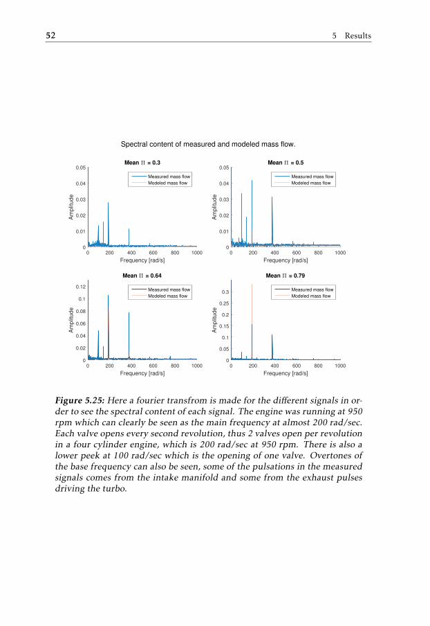
52 5 Results
0 200 400 600 800 1000
Frequency [rad/s]
0
0.01
0.02
0.03
0.04
0.05
Am
plit
ude
Mean Π = 0.3
Measured mass flow
Modeled mass flow
0 200 400 600 800 1000
Frequency [rad/s]
0
0.01
0.02
0.03
0.04
0.05
Am
plit
ude
Mean Π = 0.5
Measured mass flow
Modeled mass flow
0 200 400 600 800 1000
Frequency [rad/s]
0
0.02
0.04
0.06
0.08
0.1
0.12
Am
plit
ude
Mean Π = 0.64
Measured mass flow
Modeled mass flow
Spectral content of measured and modeled mass flow.
0 200 400 600 800 1000
Frequency [rad/s]
0
0.05
0.1
0.15
0.2
0.25
0.3
Am
plit
ude
Mean Π = 0.79
Measured mass flow
Modeled mass flow
Figure 5.25: Here a fourier transfrom is made for the different signals in or-der to see the spectral content of each signal. The engine was running at 950rpm which can clearly be seen as the main frequency at almost 200 rad/sec.Each valve opens every second revolution, thus 2 valves open per revolutionin a four cylinder engine, which is 200 rad/sec at 950 rpm. There is also alower peek at 100 rad/sec which is the opening of one valve. Overtones ofthe base frequency can also be seen, some of the pulsations in the measuredsignals comes from the intake manifold and some from the exhaust pulsesdriving the turbo.
6Conclusion
In this chapter the conclusion and summary of this master’s thesis is presented,along with some suggestions for future work.
6.1 Summary
This master’s thesis have focused on the standard isentropic adiabatic compress-ible flow equation for a nozzle and evaluated how well the assumptions madewhen deriving the equation fits the conditions for a throttle in a combustion en-gine. Already in (Andersson, 2005) and among others, measurements shows thatsome of the assumptions made when deriving the standard compressible equa-tion might have been too much of a simplification. Such measurements havebeen done in this master’s thesis as well and the same effect has been found. Herefollows a short list of the assumptions which were investigated.
• The first assumption which was investigated was the usage of a mean pres-sure ratio when calculating the mass flow. Typical intake manifold pul-sations were measured with fast sampling sensors and the resulting pres-sure ratio was inserted into a simulink model which calculated the meanmass flow and presented a Ψ -function. This was done for three differentengine loads, thus three different amplitudes of the pulsations. The resultshows that for typical intake manifold pulsations the resulting Ψ -functiondo not deviate as much as shown in (Andersson, 2005). The deviation isalso largest at pressure ratios close to one which is the opposite as the mea-surements shows in (Andersson, 2005), thus the assumption that the flowis steady is good enough, at least for the throttle. However where pressureratio is close to one and the pulsations are larger this assumption leads tomodeling errors, such as for the long route egr valve.
53
54 6 Conclusion
• The second assumption is that the flow is both adiabatic and isentropic, adi-abatic means no heat exchange with the surrounding, and isentropic meansconstant entropy. Both these assumptions correlates to the internal energyof the gas and are therefore lumped into one assumption, this since it needsextensive tests to show where the energy is coming from if it exchanges en-ergy with the surrounding or energy is generated within. Where the energyis coming from is not that interesting, the interesting part is how it affectsthe flow. Instead of this assumption an efficiency term is introduced, whichcan simplified be described as the amount of useful enthalpy drop dividedby the ideal enthalpy drop over the valve. A new equation is derived withthis in mind, in appendix B, the results are promising and the deviation inthe ideal Ψ -function can be explained by this. The ANSYS analysis indi-cates a generation of entropy in the streamlines close to the wall, howeverno generation of entropy is seen in the other streamlines which does not goalong with the results from the equation and the good fit to the data. Thiscan be explained by the simplification ANSYS does when calculating turbu-lent flow, due to lack in computational power and knowledge about ANSYSfluent the simulation were not complex enough to capture the generationof entropy. However the model fits well to the data taken in a flow benchand the efficiency term is around 92.5% which is in line with what is statedin (Çengel et al., 2012).
• The third assumption is that the effective area function Aef f (α) only de-pends on the throttle plate angle α and is not dependant on the pressureratio Aef f (α,Π). Due to the difficulty in pinpointing where in the modelthe deviation is coming from, if it is the Ψ -function or the area functionthis has only been investigated by looking at the streamlines in the ANSYSsimulation. The streamlines in the ANSYS analysis does not indicate thatthe streamlines are contracting at higher pressure ratios, however here isa lot of uncertainties due to the lack of computational power once againwhich could not simulate pressure ratios below 0.7. Due to the limitationsand large uncertainties in this method it is not investigated further whenthe second assumption seems to be the problem in the model.
The improved model which does not assume adiabatic and isentropic flowhave improved the modeling accuracy by decreasing the relative error for boththe effective area function by 7% and for the Ψ -function by 32%. The dataused here is 236 different stationary operating points for the Volvo engine in theengine-lab, a so called engine map.
Furthermore this master’s thesis introduces a dynamic flow model which uti-lizes the 1-D momentum equation to add an extra dynamic term to the regularmass flow model. The dynamic equation handles back flow by shifting the sign ofthe flow and replacing pressure and temperature with the upstream pressure andtemperature. The model is intended for places where the pressure ratio is closeto one and there is large pulsations, meaning the pulsating effect is not negligiblehere. This occurs in for example the exhaust and more specific the long routeegr valve. However due to the harsh conditions in the exhaust and not being

6.2 Future Work 55
able to measure the flow over such a valve the measurements where taken on athrottle. The pulsations are not as big here and there is an intercooler and a turboinfluencing the measurements in-between of the throttle and the fast samplingMAF-sensor the connection between the dynamic flow model and the measureddata was never made. The spectrum of the signals where investigated but in orderto implement and finding the terms in the dynamic model more work is needed.
6.2 Future Work
The time spent on this thesis has unfortunate come to an end, however this in-triguing subject leaves if possible more to think about now than before the workstarted. The two main working directions in the future is proposed here.
6.2.1 Ψ -function
In order to be certain that the reason for the deviation in the standard Ψ -functionis the generation of entropy further analysis is needed. This can preferable bedone by someone who have more knowledge in ANSYS fluent and have access toa super computer. This will show if there is a generation of entropy or if it is someother effect, however this might not be of interest since the new model correlateswell with the data. Investigations if it is sufficient to assume the efficiency to beseen as a constant or if there is a need for an efficiency function, some work havebeen done in this thesis on this subject but more is perhaps needed.
6.2.2 Dynamic Flow Model
The dynamic flow model needs to be investigated further, for example how thecoefficients should be extracted from measurements and how the measurementsshould be done, both practical and in theory in order to easily obtain the coef-ficients needed for an implementation of the model. Another solution is alsoto model the dynamics of the system between measuring point and the throttlevalve, which makes it possible to estimate the instantaneous flow past the throt-tle. When this is done the model can be evaluated. Measurements are preferabledone under such conditions for which the model is intended, as in a long routeegr system of a combustion engine. However the model is hopefully a good start-ing point when modeling the pulsating and back flowing behaviour of valvessuch as the long route egr.


Appendix

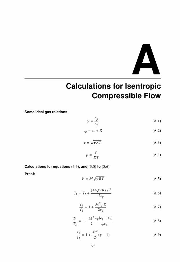
ACalculations for Isentropic
Compressible Flow
Some ideal gas relations:
γ =cpcv
(A.1)
cp = cv + R (A.2)
c =√γRT (A.3)
ρ =p
RT(A.4)
Calculations for equations (3.3), and (3.5) to (3.6).
Proof:V = M
√γRT (A.5)
T1 = T2 +(M
√γRT2)2
2cp(A.6)
T1
T2= 1 +
M2γR
2cp(A.7)
T1
T2= 1 +
M2
2
cp(cp − cv)
cvcp(A.8)
T1
T2= 1 +
M2
2(γ − 1) (A.9)
59
60 A Calculations for Isentropic Compressible Flow
T1
T2= 1 +
γ − 12
M2 (A.10)
Calculations for equations (3.3), (3.4), and (3.5) to (3.7).
Proof:T1
T2= 1 +
γ − 12
M2 (A.11)
T2
T1=
(p2
p1
) (γ−1)γ
(A.12)
1 +γ − 1
2M2
−1
=(p2
p1
) (γ−1)γ
(A.13)
1 +γ − 1
2M2
−1(p1
p2
) (γ−1)γ
= 1 (A.14)
(p1
p2
) (γ−1)γ
=
1 +γ − 1
2M2
(A.15)
p1
p2=
1 +γ − 1
2M2
γγ−1
(A.16)
Calculations for equations (3.6), (3.7), and (3.8) to (3.9).
Proof:
mideal = ρAV =p2
RT2AV =
p2
RT2AM
√γRT2 =
p2√RT2
AM√γ (A.17)
mideal =
p1
1 + γ−12 M2
−γγ−1
√√RT1
1 + γ−12 M2
−1AM√γ (A.18)
mideal =p1√RT1
AM√γ
1 +γ − 1
2M2
−γγ−1
1 +γ − 1
2M2
12
(A.19)
mideal =p1√RT1
AM√γ
1 +γ − 1
2M2
−(γ+1)
2(γ−1)
(A.20)

61
Calculations for equation (3.9) to (3.10).
Proof:Π =
(p2
p1
)(A.21)
M =Vc
=
√2cp(T1 − T2)√
γRT2(A.22)
M =
√√2cpγR
Π− γ−1γ − 1
(A.23)
M =
√√ 2cpcpcv
(cp − cv)
Π− γ−1γ − 1
(A.24)
M =
√√ 2γ − 1
Π− γ−1γ − 1
(A.25)
mideal =p1√RT1
A√γ
√√ 2γ − 1
Π− γ−1γ − 1
1 +γ − 1
22
γ − 1
Π− γ−1γ − 1
−(γ+1)
2(γ−1)
(A.26)
mideal =p1√RT1
A√γ
√√ 2γ − 1
Π− γ−1γ − 1
Π− γ−1γ
−(γ+1)
2(γ−1)
(A.27)
mideal =p1√RT1
A√γ
√√ 2γ − 1
Π− γ−1γ − 1
Πγ+12γ
(A.28)
mideal =p1√RT1
A
√√ 2γγ − 1
Π− γ−1γ − 1
Πγ+1γ
(A.29)
m =p1√RT1
A
√2γγ − 1
(Π
2γ −Π
γ+1γ
)(A.30)


BCalculations for Non-isentropic
Compressible Flow
Proof:
ηN =V 2
2a
V 22s
(B.1)
ηN =T1 − T2a
T1 − T2s(B.2)
ηN =T1 − T2a
T1 − T1
(p2p1
) γ−1γ
(B.3)
ηN =1 − T2a
T1
1 −(p2p1
) γ−1γ
(B.4)
T2a
T1= 1 − ηN + ηN
(p2
p1
) γ−1γ
︸ ︷︷ ︸The effective pressure quota ΠηN
(B.5)
Substituting the velocity in equation (3.3) is done the same way as for isen-tropic flow.
T1
T2a= 1 +
γ − 12
M2 (B.6)
Substituting the temperature with velocity in equation (3.18) is done as fol-lows.
63

64 B Calculations for Non-isentropic Compressible Flow
Proof:T2a
T1= 1 − ηN
(1 −
(p2
p1
) γ−1γ
)(B.7)
1 +γ − 1
2M2
−1
= 1 − ηN(1 −
(p2
p1
) γ−1γ
)(B.8)
1ηN− 1
ηN
1 + γ−12 M2
= 1 −
(p2
p1
) γ−1γ
(B.9)
1 − 1ηN
+1
ηN
1 + γ−12 M2
=
(p2
p1
) γ−1γ
(B.10)
ηN
1 + γ−12 M2
− 1 + γ−12 M2
+ 1
ηN
1 + γ−12 M2
=
(p2
p1
) γ−1γ
(B.11)
(p1
p2
) γ−1γ
=
ηN
1 + γ−12 M2
(ηN − 1)
1 + γ−12 M2
+ 1
(B.12)
(p1
p2
)=
ηN
1 + γ−12 M2
(ηN − 1)
1 + γ−12 M2
+ 1
γγ−1
(B.13)
(p1
p2
)=
1 +γ − 1
2M2
γγ−1
ηN
(ηN − 1)
1 + γ−12 M2
+ 1
γγ−1
︸ ︷︷ ︸New part of formula with regard to efficiency
(B.14)
Furthermore the same approach as for isentropic mass flow is used, howeverthe pressure quota when calculating the Mach number are to be replaced withthe effective pressure quota ΠηN .

65
M =
√√ 2γ − 1
1ΠηN
− 1
(B.15)
For simplicity the Mach number in the new term in equation (B.14) is substi-tuted first.
Proof: ηN
(ηN − 1)
1 + γ−12 M2
+ 1
γγ−1
(B.16)
ηN
(ηN − 1)
1 + γ−12
2γ−1
1ΠηN− 1
+ 1
γγ−1
(B.17)
ηN(ηN − 1) 1
ΠηN+ 1
γγ−1
(B.18)
The mass flow calculations without the new term is:
Proof:
mpart =p1√RT1
A√γ
√√ 2γ − 1
Π−1ηN − 1
1 +γ − 1
22
γ − 1
Π−1ηN − 1
−(γ+1)
2(γ−1)
(B.19)
mpart =p1√RT1
A√γ
√√ 2γ − 1
Π−1ηN − 1
Π−1ηN
−(γ+1)
2(γ−1)
(B.20)
mpart =p1√RT1
A√γ
√√ 2γ − 1
Π−1ηN − 1
Π (γ+1)(γ−1)ηN
(B.21)
mpart =p1√RT1
A
√2γγ − 1
(Π
2(γ−1)ηN −Π
(γ+1)(γ−1)ηN
)(B.22)
Adding the previous calculated part the full equation for the mass flow withregard to the isentropic efficiency is obtained.
mf ull =p1√RT1
A
√2γγ − 1
(Π
2(γ−1)ηN −Π
(γ+1)(γ−1)ηN
) ηN(ηN − 1)( 1
ΠηN+ 1)
γγ−1
(B.23)

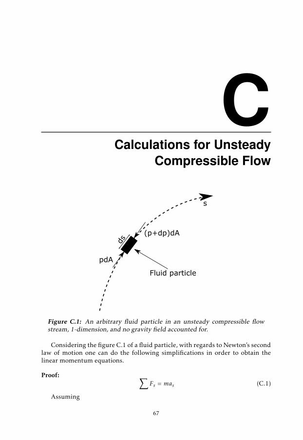
CCalculations for Unsteady
Compressible Flow
ds
pdA
(p+dp)dA
s
Fluid particle
Figure C.1: An arbitrary fluid particle in an unsteady compressible flowstream, 1-dimension, and no gravity field accounted for.
Considering the figure C.1 of a fluid particle, with regards to Newton’s secondlaw of motion one can do the following simplifications in order to obtain thelinear momentum equations.
Proof: ∑Fs = mas (C.1)
Assuming
67

68 C Calculations for Unsteady Compressible Flow
pdA − (p + dp)dA = m(∂vds∂sdt
+∂v∂t
)(C.2)
− dpdA = ρdsdA(∂v∂sv +
∂v∂t
)(C.3)
1ρ
∂p
∂x+ v
∂v∂x
+∂v∂t
= 0 (C.4)
Which is how the 1-D linear momentum equation in fluid mechanics is com-monly presented. Now substituting the density with the isentropic relation thefollowing calculations can be made.
ρ
ρ0=
( pp0
) 1γ
(C.5)
1ρ0
(p0
p
) 1γ ∂p
∂x+ v
∂v∂x
+∂v∂t
= 0 (C.6)
Furthermore integrating and assuming that v0 ≈ 0.
p1γ
0ρ0
xt∫x0
1
p1γ
dp +v2t
2+
xt∫x0
∂v∂tdx = 0 (C.7)
Replacing the velocity with mass flow.
v =mρA
=mρ0A
(p0
p
) 1γ
(C.8)
p1γ
0ρ0
xt∫x0
1
p1γ
dp +m2
2ρ20A
2t
(p0
pt
) 2γ
+p
1γ
0ρ0
xt∫x0
1A∂∂t
mp
1γ
dx = 0 (C.9)
p1γ
0ρ0
γ
γ − 1
(pγ−1γt − p
γ−1γ
0
)+
m2
2ρ20A
2t
(p0
pt
) 2γ
+p
1γ
0ρ0
xt∫x0
1A∂∂t
mp
1γ
dx = 0 (C.10)
Assuming that the dependency of x on m(x), and p(x) are negligible in the integralterm, the integral can be simplified. Same assumptions is made in (Kiwan et al.,2016) and the result is promising.
p1γ
0ρ0
γ
γ − 1
(pγ−1γt − p
γ−1γ
0
)+
m2
2ρ20A
2t
(p0
pt
) 2γ
+p
1γ
0ρ0
∂∂t
mp
1γ
0
xt∫x0
dxA
= 0 (C.11)

69
Substituting the density with ρ0 = p0T0R
and and pressure with Π = ptp0
.
p1γ
0γ
γ − 1
(pγ−1γt − p
γ−1γ
0
)+m2T0R
2p0A2t
(p0
pt
) 2γ
+ p1γ
0∂∂t
mp
1γ
0
xt∫x0
dxA
= 0 (C.12)
γ
γ − 1
(pγ−1γt − p
γ−1γ
0
)+m2T0R
2A2t
(p 1−γγ
0
p2γt
)+∂∂t
mp
1γ
0
xt∫x0
dxA
= 0 (C.13)
p20Π
2γ
γ
γ − 1
(Π
γ−1γ − 1
)+m2T0R
2A2t
+ Π2γ p
γ+1γ
0∂∂t
mp
1γ
0
xt∫x0
dxA
= 0 (C.14)
p20A
2t
T0R
2γγ − 1
(Π
2γ −Π
γ+1γ
)= m2 +
2A2t
T0RΠ
2γ p
γ+1γ
0∂∂t
mp
1γ
0
xt∫x0
dxA
(C.15)
If the last term, containing the dynamics of the flow, in above equation (C.15) isneglected, and At is replaced by some area function of the valve opening Aef f (α)and Cd is introduced to account for unknown losses the steady compressible ori-fice equation is acquired.
Aef f Cdp0√T0R
√2γγ − 1
(Π
2γ −Π
γ+1γ
)= m (C.16)
Since the geometry in the valve changes depending on the opening angle it ismore convenient to replace the integral therm with a dynamic area function, Adynwhich have to be determined by dynamic tests. Assuming that the change of p0with time is negligible compared to the mass flow change of time, the p0 termcan be extracted from the time derivative. Resulting in the following equationfor unsteady, compressible, isentropic, adiabatic, mass flow, similar to the steadycompressible equation but with a term for the inertia of the gas.
A2ef f C
2d
p20
T0R
2γγ − 1
(Π
2γ −Π
γ+1γ
)= m2 + AdynA
2ef f C
2d
2p0
T0RΠ
2γ∂m∂t
(C.17)

Bibliography
Per Andersson. Air Charge Estimation in Turbocharged Spark Ignition Engines.PhD thesis, Linköpings Universitet, December 2005. Cited on pages iii, 2, 3, 6,9, 11, 12, 20, 27, 31, 41, and 53.
David Chalet, Alexandre Mahe, Jérôme Migaud, and Jean-François Hetet. Afrequency modelling of the pressure waves in the inlet manifold of internalcombustion engine. Applied Energy, 88(9):2988 – 2994, 2011. ISSN 0306-2619. URL http://www.sciencedirect.com/science/article/pii/S0306261911002066. Cited on page 7.
Ivan Criscuolo, Oskar Leufven, Andreas Thomasson, and Lars Eriksson. Model-based boost pressure control with system voltage disturbance rejection. InIFAC World Congress, Milano, Italy, 2011. Cited on page 11.
Lars Eriksson and Lars Nielsen. Modeling and Control of Engines and Drivelines.John Wiley & Sons, 2014. Cited on pages 6, 8, 9, 10, 11, 12, and 27.
Torkel Glad and Lennart Ljung. Reglerteori : flervariabla och olinjära metoder.Lund : Studentlitteratur, 2003, 2003. ISBN 9144030037. Cited on page 11.
Torkel Glad and Lennart Ljung. Reglerteknik : grundläggande teori. Lund :Studentlitteratur, 2006, 2006. ISBN 9144022751. Cited on page 11.
Elbert Hendricks, Alain Chevalier, Michael Jensen, Spencer C. Sorenson, DaveTrumpy, and Joe Asik. Modelling of the intake manifold filling dynamics. InSAE Technical Paper. SAE International, 02 1996. doi: 10.4271/960037. URLhttp://dx.doi.org/10.4271/960037. Cited on pages 2 and 9.
Ingerid Andersson Dan Loyd Karl Storck, Matts Karlsson. Formelsamling itermo- och fluiddynamik. Institutionen för ekonomisk och industriell utveck-ling Tekniska högskolan vid Linköpings universitet, 2012. Cited on pages 5and 36.
Rani Kiwan, Anna G. Stefanopoulou, Jason Martz, Gopichandra Surnilla,Imtiaz Ali, and Daniel Joseph Styles. Effects of differential pressure
71
72 Bibliography
measurement characteristics on low pressure-egr estimation error in si-engines*. IFAC-PapersOnLine, 49(11):722 – 729, 2016. ISSN 2405-8963. URL http://www.sciencedirect.com/science/article/pii/S2405896316314550. 8th {IFAC} Symposium on Advances in AutomotiveControl {AAC} 2016Norrköping, Sweden, 20—23 June 2016. Cited on pages 8,22, and 68.
Erik Klasén. Modeling and estimation of long route EGR mass flow in a tur-bocharged gasoline engine. Master’s thesis, Linköping University, SE-581 83Linköping, 2016. Cited on page 6.
Oskar Leufven and Lars Eriksson. Measurement, analysis and modeling of cen-trifugal compressor flow for low pressure ratios. International Journal of En-gine Research, 153(2):153–168, February 2016. Cited on page 11.
Oskar Leufvén and Lars Eriksson. A surge and choke capable com-pressor flow model—validation and extrapolation capability. Con-trol Engineering Practice, 21(12):1871 – 1883, 2013. ISSN 0967-0661. URL http://www.sciencedirect.com/science/article/pii/S0967066113001354. Cited on page 11.
Bohan Liang and Robin Holmbom. Boost control with turbo speed sensor andelectric wastegate. Master’s thesis, Linköping University, SE-581 83 Linköping,2016. Cited on pages 9 and 11.
James Lighthill. Waves in fluids. Cambridge mathematical library. Cambridge :Cambridge Univ. Press, 2001, 2001. ISBN 0521010454. Cited on pages 7 and 8.
Lennart Ljung and Torkel Glad. Modellbygge och simulering. Lund : Studentlit-teratur, 2004, 2004. ISBN 9144024436. Cited on page 9.
X. Llamas and L. Eriksson. Parameterizing compact and extensible compressormodels using orthogonal distance minimization. Journal of Engineering forGas Turbines and Power, 139(1), 2017. ISSN 15288919. Cited on page 11.
V Macián, J M Luján, V Bermúdez, and C Guardiola. Exhaust pressure pulsationobservation from turbocharger instantaneous speed measurement. Measure-ment Science and Technology, 15(6):1185, 2004. URL http://stacks.iop.org/0957-0233/15/i=6/a=020. Cited on page 8.
Svante Gunnarsson Peter Lindskog Lennart Ljung Johan Löfberg Tomas McK-elvey Anders Stenman Martin Enqvist, Torkel Glad and Jan-Erik Strömberg.IndustriellReglerteknik Kurskompendium. Bokakademin Linköping, 2014.Cited on page 11.
A. Mehmood, S. Laghrouche, and M. El Bagdouri. Nonlinear modeling of the{VNT} pneumatic actuator with aero-dynamic force. {IFAC} ProceedingsVolumes, 43(7):518 – 523, 2010. ISSN 1474-6670. URL http://www.sciencedirect.com/science/article/pii/S1474667015368816.6th {IFAC} Symposium on Advances in Automotive Control. Cited on page 10.

Bibliography 73
H. Ockendon. Waves and compressible flow. Texts in applied mathematics: v. 47.New York ; London : Springer, 2003., 2003. ISBN 038740399X. Cited on page7.
Bernhard Semlitsch, Yue Wang, and Mihai Mihăescu. Flow effects dueto pulsation in an internal combustion engine exhaust port. En-ergy Conversion and Management, 86:520 – 536, 2014. ISSN 0196-8904. URL http://www.sciencedirect.com/science/article/pii/S0196890414005597. Cited on page 8.
Stephanie Stockar, Marcello Canova, Baitao Xiao, Julia Buckland, and WenDai. Modeling for estimation of wave action in multi-cylinder turbocharged{SI} engines. IFAC-PapersOnLine, 49(11):708 – 713, 2016. ISSN 2405-8963. URL http://www.sciencedirect.com/science/article/pii/S2405896316314537. 8th {IFAC} Symposium on Advances in AutomotiveControl {AAC} 2016Norrköping, Sweden, 20—23 June 2016. Cited on page 8.
Andreas Thomasson and Lars Eriksson. Effects of pulsating flow on mass flow bal-ance and surge margin in parallel turbocharged engines. In The 56th Confer-ence on Simulation and Modelling (SIMS 56), Linköping, Sweden, 2015. Citedon page 9.
Andreas Thomasson, Oskar Leufvén, Ivan Criscuolo, and Lars Eriksson. Mod-eling and validation of a boost pressure actuation system, for a series sequen-tially turbocharged {SI} engine. Control Engineering Practice, 21(12):1860 –1870, 2013. ISSN 0967-0661. URL http://www.sciencedirect.com/science/article/pii/S0967066113000063. Cited on page 10.
Zhenyi Yang. Exhaust pressure waves in diesel engines and the impacts on af-tertreatment sprays. 2015. Cited on page 7.
Yunus A. Çengel, Robert H. Turner, John M. Cimbala, and Mehmet Kano?lu. Fun-damentals of thermal-fluid sciences. Singapore : McGraw-Hill, c2012., 2012.ISBN 9780071325110. Cited on pages 6, 8, 13, 16, 18, and 54.