riemann problem for dissociating hydrogen gas...the riemann problem of gasdynamics is very important...
TRANSCRIPT
POLITECNICO DI MILANO
Facoltà di Ingegneria IndustrialeCorso di Laurea in Ingegneria Aeronautica
Riemann problem for dissociatinghydrogen gas
Relatore: Prof. Luigi Quartapelle
Enrico Rinaldi 729906
Anno Accademico 2009/2010

Contents
1 Introduction 3
2 Thermodynamics of hydrogen gas at equilibrium 5
2.1 Helmholtz potential . . . . . . . . . . . . . . . . . . . . . . . . . . 5
2.2 Equilibrium dissociation . . . . . . . . . . . . . . . . . . . . . . . 5
2.3 Energy equation of state . . . . . . . . . . . . . . . . . . . . . . . . 6
2.4 Entropy equation of state . . . . . . . . . . . . . . . . . . . . . . . 7
2.5 Thermodynamic properties . . . . . . . . . . . . . . . . . . . . . . 7
2.5.1 Pressure . . . . . . . . . . . . . . . . . . . . . . . . . . . . . 8
2.5.2 Specific heats . . . . . . . . . . . . . . . . . . . . . . . . . . 8
2.5.3 Sound speed . . . . . . . . . . . . . . . . . . . . . . . . . . 12
2.5.4 Fundamental derivative of gasdynamics . . . . . . . . . . . .12
3 Simplified hydrogen model 15
3.1 Dissociation equation and equilibrium properties . . . .. . . . . . 15
3.2 Comparison between the models . . . . . . . . . . . . . . . . . . . 17
4 Riemann problem for dissociating gas 21
4.1 Eigenstructure of Euler equations . . . . . . . . . . . . . . . . . .. 21
4.2 Linear degeneracy and genuine nonlinearity . . . . . . . . . .. . . 22
4.3 Contact discontinuity . . . . . . . . . . . . . . . . . . . . . . . . . 23
4.4 Rarefaction wave . . . . . . . . . . . . . . . . . . . . . . . . . . . 24
4.5 Shock wave . . . . . . . . . . . . . . . . . . . . . . . . . . . . . . 25
4.6 Structure of the Riemann problem . . . . . . . . . . . . . . . . . . 27
5 Results 31
5.1 Hugoniot curves . . . . . . . . . . . . . . . . . . . . . . . . . . . . 31
5.2 Shock waves . . . . . . . . . . . . . . . . . . . . . . . . . . . . . . 32
5.3 Rarefaction waves . . . . . . . . . . . . . . . . . . . . . . . . . . . 36
5.4 Mixed solution . . . . . . . . . . . . . . . . . . . . . . . . . . . . 39
iii
iv Contents
6 Conclusions 41
A Partition functions for molecular and atomic hydrogen 43
A.1 The hydrogen molecule . . . . . . . . . . . . . . . . . . . . . . . . 44
A.1.1 Translation . . . . . . . . . . . . . . . . . . . . . . . . . . . 44
A.1.2 Rotation . . . . . . . . . . . . . . . . . . . . . . . . . . . . . 44
A.1.3 Vibration . . . . . . . . . . . . . . . . . . . . . . . . . . . . 45
A.1.4 Roto-vibration . . . . . . . . . . . . . . . . . . . . . . . . . 46
A.1.5 Electrons . . . . . . . . . . . . . . . . . . . . . . . . . . . . 49
A.1.6 Complete partition function for the molecule . . . . . . .. . 49
A.2 The hydrogen atom . . . . . . . . . . . . . . . . . . . . . . . . . . 50
References 51
List of Figures v
List of Figures
1 Specific heats for the RVD gas model (1) . . . . . . . . . . . . . . . 9
2 Specific heats for the RVD gas model (2) . . . . . . . . . . . . . . . 10
3 Specific heats for ortho-, para- and normal hydrogen . . . . . .. . . 11
4 Sound speed for the RVD gas model . . . . . . . . . . . . . . . . . 12
5 Fundamental derivative of gasdynamics for the RVD gas model . . . 13
6 RVD-VD-HC comparison onα . . . . . . . . . . . . . . . . . . . . 17
7 RVD-VD-HC comparison on the pressure . . . . . . . . . . . . . . 18
8 RVD-VD-HC comparison oncv . . . . . . . . . . . . . . . . . . . . 19
9 RVD-VD comparison oncv . . . . . . . . . . . . . . . . . . . . . . 19
10 RVD-VD-HC comparison on the sound speed . . . . . . . . . . . . 20
11 Hugoniot curves and dissociation coefficient after the shock . . . . . 32
12 Two shock waves with partial dissociation . . . . . . . . . . . . .. 34
13 Two shock waves in the low temperature range . . . . . . . . . . . .35
14 Two rarefaction waves with partial dissociation . . . . . . .. . . . 37
15 Two rarefaction waves in the low temperature range . . . . . .. . . 38
16 Riemann probelm with both shock and rarefaction wave . . . .. . . 40
17 Harmonic vs Morse potential . . . . . . . . . . . . . . . . . . . . . 46
18 Roto-vibrational eigenvalues: numerical comparisons .. . . . . . . 47
19 Roto-vibrational eigenvalues: experimental data comparison . . . . 47
20 Cutoff curve for roto-vibrational spectrum . . . . . . . . . . .. . . 48

vi List of Figures

List of Tables vii
List of Tables
1 Morse parameters for H2 molecule . . . . . . . . . . . . . . . . . . 48

viii List of Tables
Sommario
L’obiettivo di questa tesi è lo studio del problema di Riemann della gasdinamica inun gas diatomico che dissocia. L’attenzione sarà concentrata sul gas di idrogeno.Nonostante l’idrogeno non sia coinvolto nelle tipiche correnti ipersoniche nellefasi di rientro atmosferico, la scelta è comunque giustificata dalle sue numeroseapplicazioni tecnologiche. Inoltre, diversi studi di carattere astrofisico coinvol-gono il gas idrogeno che attraversa un ampio intervallo di temperature fino allaionizzazione.
Da un punto di vista termodinamico l’idrogeno è molto interessante a causa delvalore piuttosto elevato della suatemperatura rotazionaleche consente agli effettidovuti alle rotazioni molecolari di manifestarsi a temperature non troppo basse.
In questo lavoro è stato utilizzato un modello termodinamico recentemente in-trodotto da Quartapelle e Muzzio [1] (si veda anche [2]) che tiene correttamente inconto l’accoppiamento tra rotazioni e vibrazioni anarmoniche della molecola H2,descritte tramite il potenziale di Morse [3]. Inoltre, la dissociazione molecolareviene rappresentata come un aspetto puramente termodinamico che avviene in se-guito a rotazioni o vibrazioni non più sostenibili, abbandonando quindi lalegge diazione di massaspesso impiegata per determinare la composizione all’equilibriodi una miscela. L’attenzione di questa tesi è rivolta all’introdurre questo concettonella risoluzione del problema di Riemann. I risultati ottenuti verranno confrontaticon quelli forniti da un modello termodinamico semplificatoche considera le ro-tazioni completamente eccitate. L’analisi non sarà limitata solamente ai valoridi temperatura elevati ai quali avviene la dissociazione, ma si rivolgerà anche aldominio delle basse temperature alle quali la distinzione tra i due modelli termodi-namici diventa marcata. Sebbene già in condizioni di dissociazione le differenze trai risultati forniti dai due modelli inducano all’utilizzo di quello completo, quandolo sguardo si sposta sulle basse temperature la scelta diventa obbligata.
Il capitolo 2 descrive il modello termodinamico completo per l’idrogeno, cheinclude l’accoppiamento tra rotazioni e vibrazioni della molecola e la sua disso-ciazione (RVD). Sono inoltre derivate le espressioni di tutte le proprietà termod-inamiche necessarie nella soluzione del problema di Riemann, come funzioni ditemperaturaT e volume specificov.
Il capitolo 3 richiama i principi fondamentali di due modelli semplificati, en-trambi caratterizzati da un trattamentoclassicodelle rotazioni. Il primo modellocondivide con quello completo le vibrazioni anarmoniche e la dissociazione (VD)mentre il secondo è basato su oscillazioni armoniche e utilizza la legge di azionedi massa per determinare la composizione del gas. Sono inoltre effettuati dei con-fronti sulle proprietà termodinamiche più importanti ottenuti con i vari modelli.
1
2 Sommario
Il capitolo 4 è la parte più originale del lavoro ed è dedicataallo studio delproblema di Riemann per un gas diatomico che dissocia. In primo luogo sonoevidenziati i tratti essenziali del problema di Riemann, come prensentato in [4]. Inseguito si fornisce una nuova e completa formulazione del problema, estesa al gasin presenza di dissociazione. Quest’ultima rende il problema matematico più com-plicato e richiede la soluzione di sistemi non lineari all’interno del ciclo principaleche determina gli stati sinistro e destro sulla discontinuità di contatto. In partico-lare, sia la soluzione dell’onda d’urto che dell’onda di rarefazione richiedono dirisolvere un sistema formato da due equazioni che sono l’equazione che definisce ilcoefficiente di dissociazione e, rispettivamente, l’equazione di Rankine–Hugonioto la condizione di entropia costante.
Nel capitolo 5 sono presentati e commentati i risultati più significativi deiproblemi di Riemann analizzati. Particolare attenzione è dedicata alle situazioniin cui la dissociazione gioca un ruolo importante, quindi alle alte temperature. Perverificare l’accuratezza dei risultati è effettuato un confronto tra quelli ottenuti conil modello RVD e VD. Inoltre, nel caso delle onde d’urto, è possibile confrontarele soluzioni con i dati forniti dalla NASA [5]. Infine viene analizzata la regione dibasse temperature sia per le onde d’urto che di rarefazione,in modo da evidenziarele differenze che scaturiscono da un differente trattamento delle rotazioni.
Il capitolo 6 riassume il lavoro fatto e le conclusioni che sipossono trarre,proponendo infine possibili sviluppi futuri.
Infine l’appendice A presenta le espressioni delle funzionidi partizione utiliz-zate nei modelli RVD e VD.
1 Introduction
The Riemann problem of gasdynamics is very important in the study of nonlinearwaves in compressible flows and it is also fundamental in the development offinite volume methods in which it occurs at every interface between two grid cells.Generally, theRiemann problem forgases with simple thermodynamicproperties isstudied. On theotherhand, taking into account moleculardissociation is mandatoryfor hypersonic flows in which the rise in temperature after the shock front leads toa modification in the chemical composition of the gas.
The aim of this work is to study the Riemann problem in a diatomic gas in thepresence of dissociation. The focus will be on the hydrogen gas. Even if the hy-drogen is not involved in typical hypersonic flows in the re-entry phase, the choiceis justified by its many technological applications (a typical Riemann problem ofgeneral interest involving hydrogen gas could be the failure of a pipe). Besidesthat, many astrophysical investigations involve the hydrogen gas encompassing awide range of temperatures up to ionization.
From a thermodynamical viewpoint, the hydrogen gas is very interesting be-cause of the fairly large value of itsrotational temperature, so that the peculiareffects of molecular rotations can manifest at not too smalltemperatures. An orig-inal and recent thermodynamic model due to Quartapelle and Muzzio [1] (see also[2]) which properly takes into account effects of rotationsand the dissociation ofthe molecule H2 will be used. The focus of the present work will be the inclusionof the dissociation as a purely thermodynamic aspect in the Riemann problem,abandoning thelaw of mass actioncommonly employed to determine the compo-sition of the gas. Furthermore, the Riemann problem in the low temperature regionwill be analyzed in order to understand the improvements stemming from the com-plete model with a coupled treatment of rotations and anharmonic vibrations, withrespect to a simplified model which considers fully excited rotations.
Chapter 2 describes the complete thermodynamic model for the hydrogen gasincluding the rotations and vibrations of the molecules andtheir dissociation (RVD)into atoms, as presented in [1, 2]. The expressions of all thethermodynamicproperties of the gas needed for formulating the Riemann problem are derived asfunctions of the temperatureT and the specific volumev.
Chapter 3 recalls the basic elements of two simplified models, both character-ized by fully excited molecular rotations. The first model shares with the completeone the anharmonic vibrations and dissociation (VD) while the second approxi-mate model is based on harmonic oscillations (HC) but must becomplemented bythe chemical law of mass action to account for molecular dissociation.
Chapter 4 is most the original contribution of the work and isdevoted to the
3
4 Chapter 1 Introduction
study of the Riemann problem for a dissociating diatomic ideal gas. First, thefundamental features of the Riemann problem of the gasdynamics are oulined, aspresented in [4]. Then a new and complete formulation of thisproblem in thecontext of a dissociating ideal gas is presented. The presence of the dissociationcoefficient makes actually the mathematical problem more difficult than for anondissociating gas and may require to solve nonlinear systems within the externalcycle which determines the states on the two sides of the contact discontinuity. Inparticular, the solution of either the rarefaction wave or the shock wave is obtainedfrom nonlinear systems of two equations representing the dissociation equation andthe condition of constant entropy or the Rankine–Hugoniot equation, respectively.
In chapter 5 the most important results of the Riemann problems are presentedand discussed. Particular attention is payed to situationsin which the dissociationplays an important role, thus high temperature values are considered. In order toverify the accuracy of the solutions, a comparison between the results obtainedby means of RVD and VD models is made. For the case of the shock waves, acomparison with data provided by NASA [5] is also possible. Finally, the domainof low temperatures is analyzed for either shock or rarefaction waves to underlinethe differences resulting from different treatment of rotations.
Chapter 6 summarizes all the work done and the results obtained, and proposessome future developments.
Finally, appendix A presents the expressions of the partition functions used forthe RVD and VD models.
2 Thermodynamics of hydrogen gas at equilibrium
This chapter recalls the basic elements of the thermodynamic model due to Quar-tapelle and Muzzio described in [1] and detailed in the appendix RV of the lecturenotes [2]. The model describes a dissociating diatomic ideal gas under the assump-tion of thermodynamic equilibrium. The internal motion of the diatomic moleculesis characterized by a complete coupling between rotations and anharmonic vibra-tions, as described in appendix A.
First the Helmholtz potential is introduced and the condition for equilibriumdissociation is considered to define the dissociation coefficientα of the diatomicgas, which is uniquely determined by the temperatureT and the specific volumev. Next, the Helmholtz potential is used to derive the equations of state for energy,entropy and other relevant thermodynamic properties, as functions ofT andv.
2.1 Helmholtz potential
As is well known, the Helmholtz potential (also referred to as Helmholtz freeenergy) is a thermodynamic potential obtained by performing a Legendre transformon the fundamental relation in the energetic representation1 in order to haveT andVas independent variables. The expression of the free energyfor the gas consideredis:
F (T, V, NH2, NH) = −NH2
kBT lneZH2
(T, V )
NH2
− NH kBT lneZH(T, V )
NH
, (2.1)
with the partition functionsZH2(T, V ) andZH(T, V ) expressed by equations (A.15)
and (A.16), respectively. Here “e” denotes the base of the natural logarithm andNH2
andNH the number of the molecules H2 and atoms H. The free energy (2.1) isa fundamental thermodynamic relation and all the thermodynamic properties of thegas can be obtained from it. Moreover, the minimum ofF defines the equilibriumcomposition of the gas which undergoes a chemical transformation.
2.2 Equilibrium dissociation
Following Zel’dovich and Raizer [8], the equilibrium composition of the gas stemsfrom two constraints which express the stationarity ofF and the conservation of
1E = E(S, V, N) with E, S, V and N = (N1, N2, . . . ) denoting respectively the internalenergy, the entropy, the volume and the total number of particles. For a complete description of thefundamental relation in both energetic and entropic form and its mathematical properties we referto [6, 7].
5
6 Chapter 2 Thermodynamics of hydrogen gas at equilibrium
the atomic constituents of the gas mixture through the relation 2NH2+ NH = NH,
whereNH denotes the (fixed) total number of constituents present either as freeatoms H or as atomic components of the molecules H2. Using this two conditionsleads to:
N2H
NH2
=Z2
H
ZH2
. (2.2)
Let us now introduce the dissociation coefficientα:
α ≡ NH2− NH2
NH2
, (2.3)
from which we can find:
NH2= (1 − α)NH2
and NH = 2αNH2. (2.4)
Substituting the partition functions (A.15) and (A.16) into the equilibriumequation (2.2) and using the relationships (2.4), gives:
α2
1 − α=
1
4
Z2H(T, V )
ZH2(T, V )
1
NH2
=t3/2 e−td/t
znucrv (t)
v
v∗d≡ β(t, v), (2.5)
with v = V / [mH2NH2
], t = T/Tv, znucrv (t) = e−De/kBTZnuc
rv (T ) andZnucrv (T ) given
by equation (A.12), and where we have introduced the constants:
1
v∗d=
(2IH + 1)2
4√
2
(g0H)2H5/2
g0H2
T 3/2v
(2πkB)3/2 u5/2
h3,
td =nmax
2 + 1/nmax,
with H the hydrogen mass in atomic unit,u = 1.660 × 10⁻²⁷ kg, and the otherquantities defined in appendix A. Solving equation (2.5) forαgives the equilibriumdissociation coefficient of the gas:
α(t, v) =1
2β(t, v)
[
√
1 + 4/β(t, v) − 1]
. (2.6)
2.3 Energy equation of state
The internal energy of the mixture is defined by the standard relation:
E = F (T, V, NH2, NH) − T
∂F (T, V, NH2, NH)
∂T, (2.7)
2.4 Entropy equation of state 7
with F given by equation (2.1). A direct calculation provides the dimensionlessspecific internal energyǫ ≡ e/[RH2
Tv] of the dissociating gas as a function oftandα:
ǫf(t, α) =3
2(1 + α) t+ (1 − α) [ǫrv(t) − td],
where the superscriptf underlines thatǫf is the energy of thefrozenmixture, namelya function also ofα as an independent variable. Moreover,ǫrv(t) = xrv(t)/zrv(t) isthe roto-vibrational contribution to the internal energy,with xrv(t) ≡ z′rv(t) t
2. Atthermodynamic equilibrium, the dissociation coefficient is given by (2.6), so thatthe specific energy depends on both the independent variables t andv:
ǫ(t, v) =3
2[1 + α(t, v)] t+ [1 − α(t, v)] [ǫrv(t) − td]. (2.8)
2.4 Entropy equation of state
The entropy is defined from the Helmholtz free energyF by:
S = −∂F (T, V, NH2, NH)
∂T. (2.9)
A direct calculation provides the dimensionless specific entropyσ ≡ s/RH2of the
dissociating gas as a function oft, v andα:
σf(t, v, α) = (1 + α)
[
5
2+
3
2ln t+ ln
(
v
v∗d
)]
+ (1 − α)σrv(t) + Υ (α) + σ0,
whereσ0 is the entropy in a reference state,σrv(t) = xrv(t)t zrv(t)
+ ln zrv(t) is the roto-vibrational contribution to the entropy andΥ (α) ≡ −2α lnα− (1− α) ln(1− α)is the contribution due to the mixing of the molecular and atomic species.
Taking into account the equilibrium dissociation leads to the entropy equationof state:
σ(t, v) = [1 + α(t, v)]
[
5
2+
3
2ln t+ ln
(
v
v∗d
)]
+ [1 − α(t, v)]σrv(t) + Υ (α(t, v)) + σ0.
(2.10)
2.5 Thermodynamic properties
From the explicit expression of the Helmholtz potential andof the equations ofstate for energy and entropy, any other thermodynamic property of the gas can bederived. Since we are interested in the equilibrium properties, hereinafter we willalways considerα = α(t, v) avoiding to write the independent variablest andv.
8 Chapter 2 Thermodynamics of hydrogen gas at equilibrium
2.5.1 Pressure
The pressure function can be obtained from the Helmholtz potential by means of
P = −kBT∂F (T, V, NH2
, NH)
∂V. (2.11)
A direct calculation leads to:
P (T, v) = (1 + α)RH2
T
v. (2.12)
It is useful to express the derivatives of the scaled pressure p = P/[RH2Tv] with
respect tot andv:
∂p(t, v)
∂t= (1 + α + tαt)
1
v,
∂p(t, v)
∂v= − (1 + α− vαv)
t
v2,
whereαt andαv denote the partial derivatives ofα(t, v). The pressure derivativesare now used to derive other thermodynamic properties that will be employed inthe solution of the Riemann problem to be discussed in chapter 4.
2.5.2 Specific heats
First, we consider the specific heat at constant volume, which is defined as thepartial derivative of the specific internal energy with respect to the temperature:
cv(T, v) =∂e(T, v)
∂T=∂ef(T, α)
∂T+∂ef(T, α)
∂ααT (T, v). (2.13)
Substituting the expressions of the derivatives of the internal energy yields:
cv(t, v)
RH2
=3
2(1 + α) + (1 − α) ǫ′rv(t) +
[
3
2t− [ǫrv(t) − td]
]
αt (2.14)
where ǫ′rv(t) = [zrv(t) yrv(t) − xrv(t)] / [t zrv(t)]2 with yrv(t) = t2 x′rv(t). The
specific heat at constant pressure is defined as follows
cP = cv − T
(
∂v
∂T
)2
P
/ (
∂v
∂P
)
T
,
where the derivative(∂v/∂T )P is obtained from the pressure equation of stateP = P (T, v) by implicit differentiation. For the case of the dissociating diatomicideal gas considered, it yields:
cP (t, v) = cv(t, v) +(1 + α + tαt)
2
1 + α− vαv. (2.15)
2.5 Thermodynamic properties 9
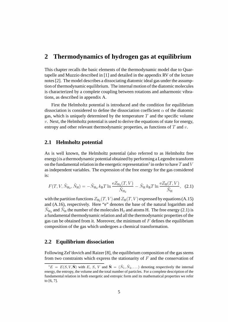
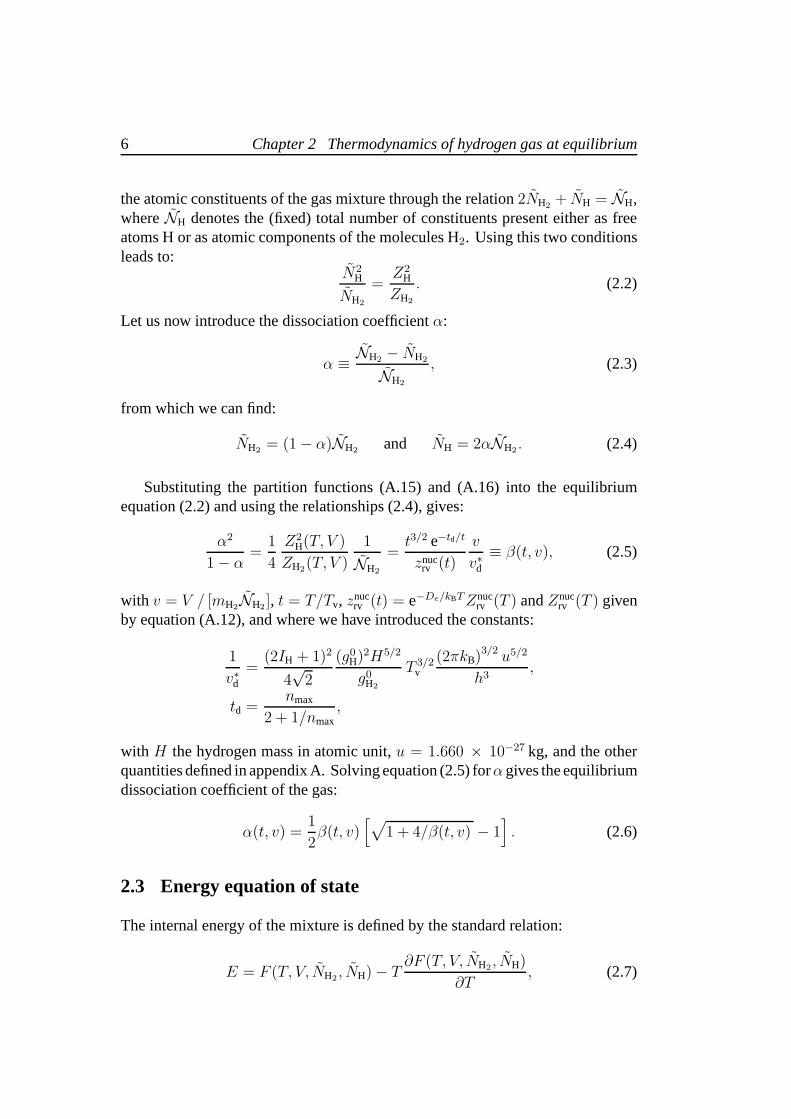
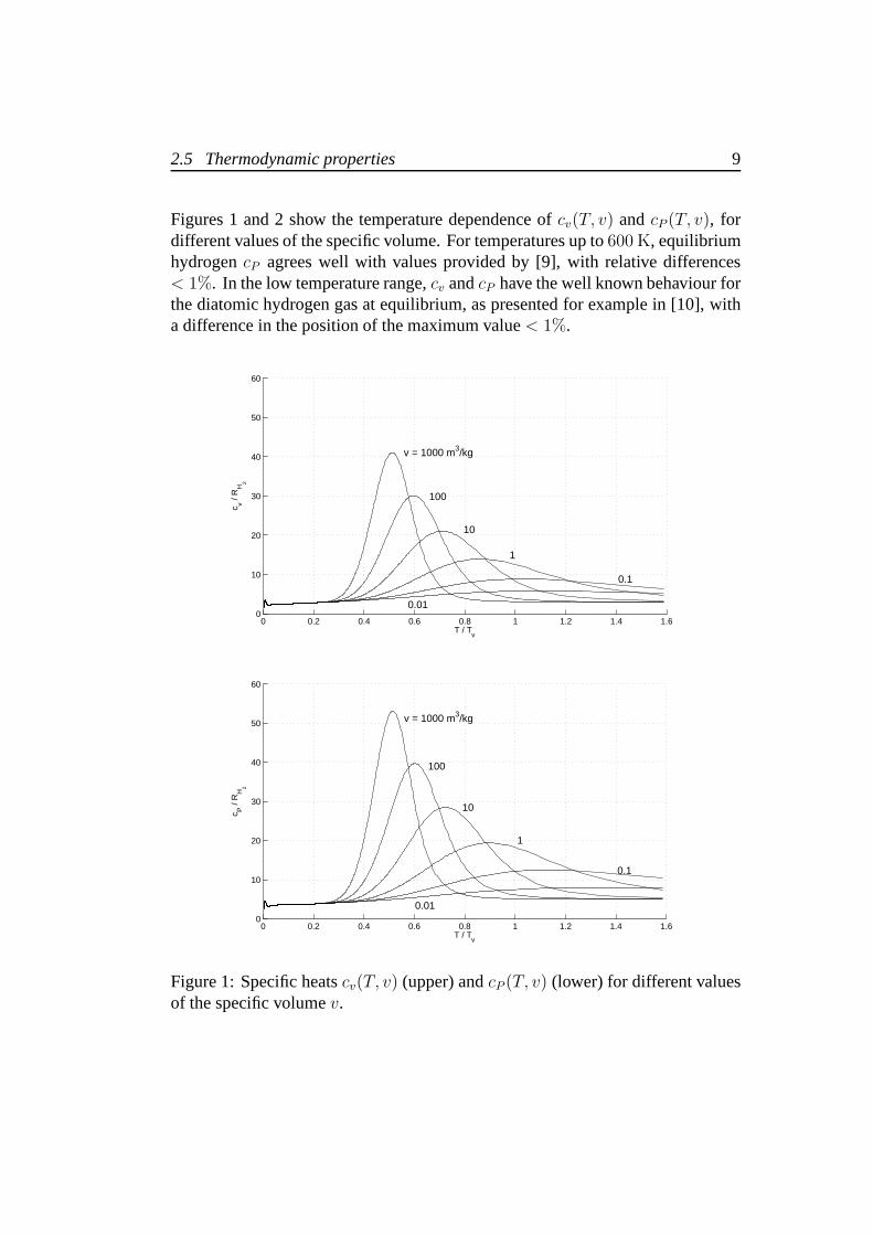
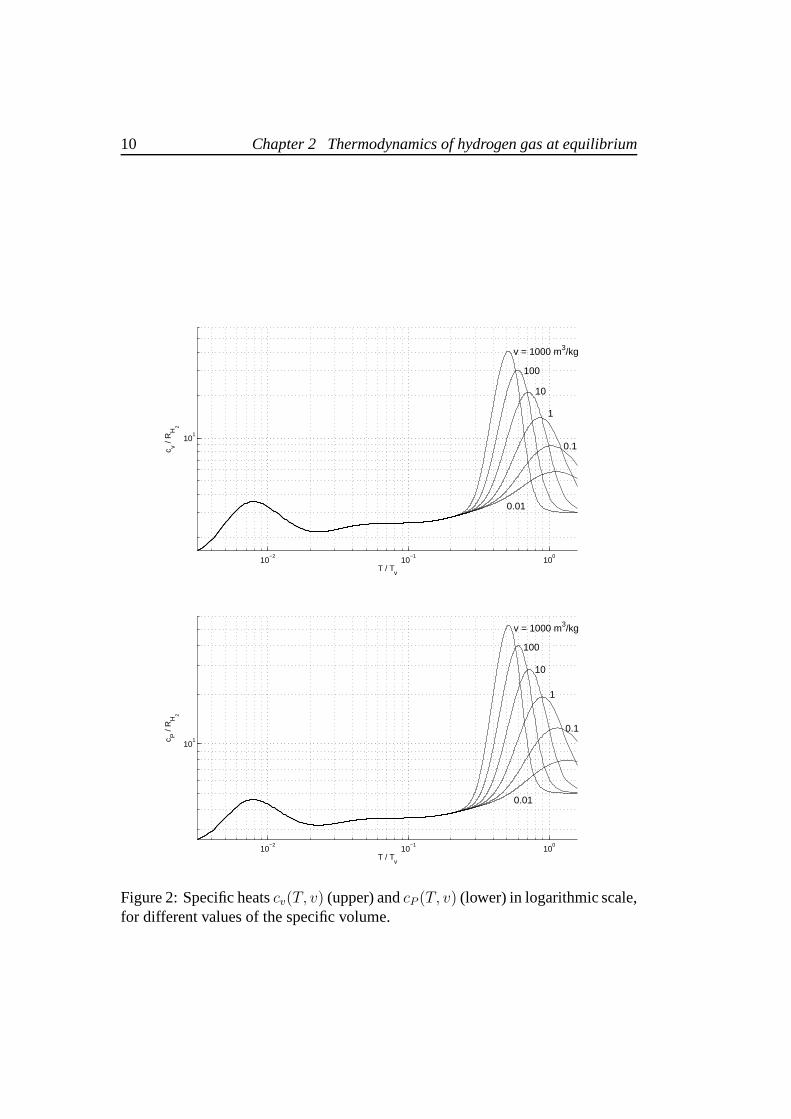
Figures 1 and 2 show the temperature dependence ofcv(T, v) andcP (T, v), fordifferent values of the specific volume. For temperatures upto 600 K, equilibriumhydrogencP agrees well with values provided by [9], with relative differences< 1%. In the low temperature range,cv andcP have the well known behaviour forthe diatomic hydrogen gas at equilibrium, as presented for example in [10], witha difference in the position of the maximum value< 1%.
0 0.2 0.4 0.6 0.8 1 1.2 1.4 1.60
10
20
30
40
50
60
T / Tv
c v / R
H2
v = 1000 m3/kg
100
10
1
0.1
0.01
0 0.2 0.4 0.6 0.8 1 1.2 1.4 1.60
10
20
30
40
50
60
T / Tv
c P /
RH
2
v = 1000 m3/kg
100
10
1
0.1
0.01
Figure 1: Specific heatscv(T, v) (upper) andcP (T, v) (lower) for different valuesof the specific volumev.
10 Chapter 2 Thermodynamics of hydrogen gas at equilibrium
10−2
10−1
100
101
T / Tv
c v / R
H2
v = 1000 m3/kg
100
10
1
0.1
0.01
10−2
10−1
100
101
T / Tv
c P /
RH
2
v = 1000 m3/kg
100
10
1
0.1
0.01
Figure 2: Specific heatscv(T, v) (upper) andcP (T, v) (lower) in logarithmic scale,for different values of the specific volume.
2.5 Thermodynamic properties 11
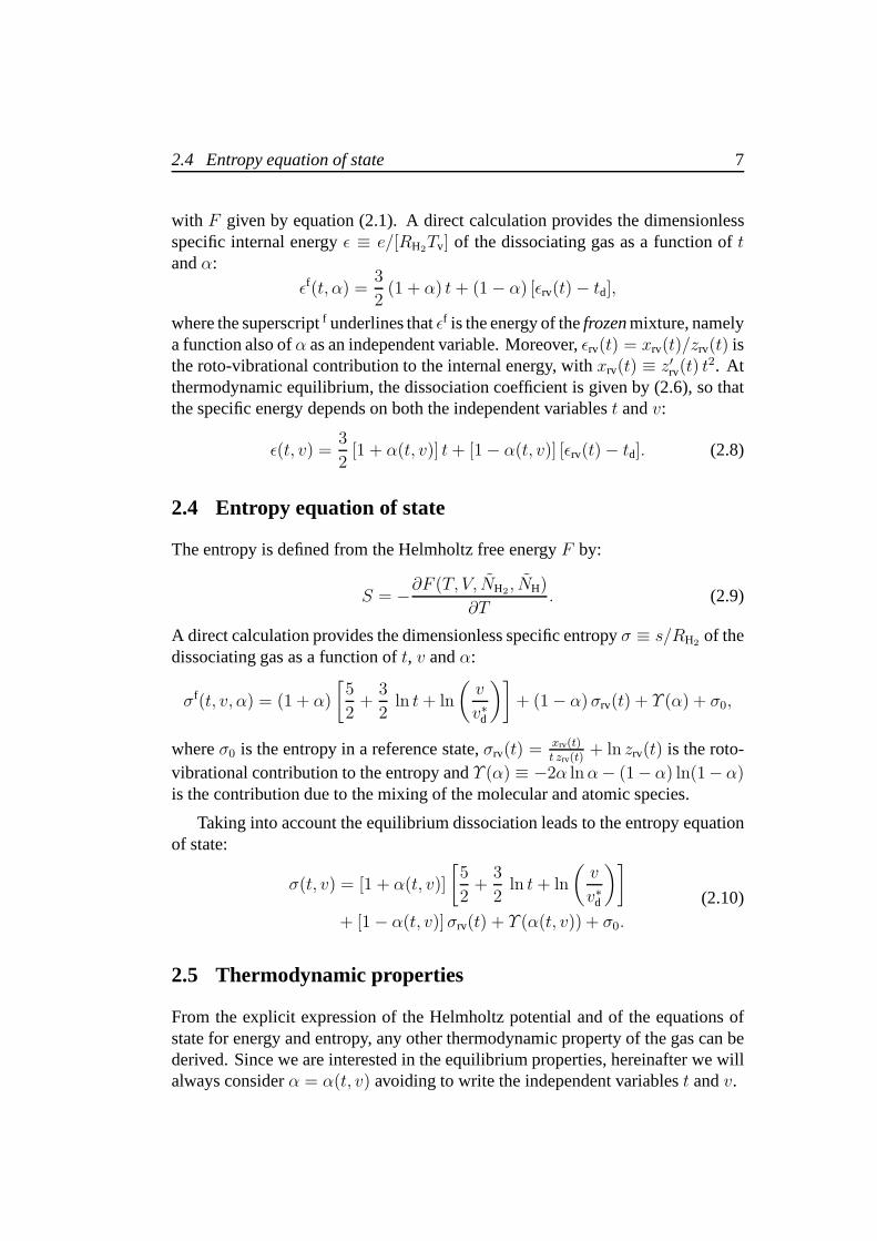
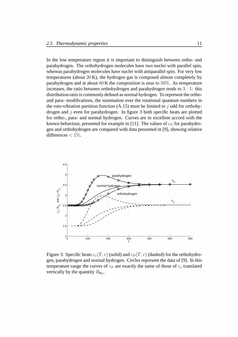
In the low temperature region it is important to distinguishbetween ortho- andparahydrogen. The orthohydrogen molecules have two nucleiwith parallel spin,whereas parahydrogen molecules have nuclei with antiparallel spin. For very lowtemperatures (about20 K), the hydrogen gas is composed almost completely byparahydrogen and at about80 K the composition is near to50%. As temperatureincreases, the ratio between orthohydrogen and parahydrogen tends to3 : 1: thisdistribution ratio is commonly defined as normal hydrogen. To represent the ortho-and para- modifications, the summation over the rotational quantum numbers inthe roto-vibration partition function (A.15) must be limited toj odd for orthohy-drogen andj even for parahydrogen. In figure 3 both specific heats are plottedfor ortho-, para- and normal hydrogen. Curves are in excellent accord with theknown behaviour, presented for example in [11]. The values of cP for parahydro-gen and orthohydrogen are compared with data presented in [9], showing relativedifferences< 1%.
0 100 200 300 400 500 6001
1.5
2
2.5
3
3.5
4
4.5
T
c v / R
H2 a
nd c
P /
RH
2
normal hydrogen
orthohydrogen
parahydrogen
cP
cv
Figure 3: Specific heatscv(T, v) (solid) andcP (T, v) (dashed) for the orthohydro-gen, parahydrogen and normal hydrogen. Circles represent the data of [9]. In thistemperature range the curves ofcP are exactly the same of those ofcv translatedvertically by the quantityRH2
.
12 Chapter 2 Thermodynamics of hydrogen gas at equilibrium
2.5.3 Sound speed
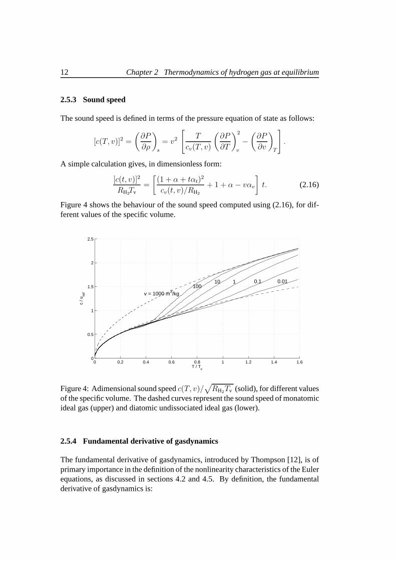
The sound speed is defined in terms of the pressure equation ofstate as follows:
[c(T, v)]2 =
(
∂P
∂ρ
)
s
= v2
[
T
cv(T, v)
(
∂P
∂T
)2
v
−(
∂P
∂v
)
T
]
.
A simple calculation gives, in dimensionless form:
[c(t, v)]2
RH2Tv
=
[
(1 + α+ tαt)2
cv(t, v)/RH2
+ 1 + α− vαv
]
t. (2.16)
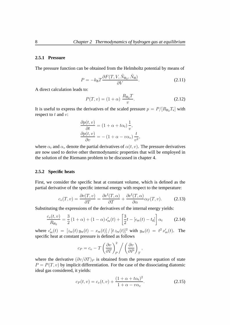
Figure 4 shows the behaviour of the sound speed computed using (2.16), for dif-ferent values of the specific volume.
0 0.2 0.4 0.6 0.8 1 1.2 1.4 1.60
0.5
1
1.5
2
2.5
T / Tv
c / u
ref v = 1000 m3/kg
10010 1 0.1 0.01
Figure 4: Adimensional sound speedc(T, v)/√
RH2Tv (solid), for different values
of the specific volume. The dashed curves represent the soundspeed of monatomicideal gas (upper) and diatomic undissociated ideal gas (lower).
2.5.4 Fundamental derivative of gasdynamics
The fundamental derivative of gasdynamics, introduced by Thompson [12], is ofprimary importance in the definition of the nonlinearity characteristics of the Eulerequations, as discussed in sections 4.2 and 4.5. By definition, the fundamentalderivative of gasdynamics is:
2.5 Thermodynamic properties 13
Γ = 1 − v
c
∂c(s, v)
∂v.
The derivative of the sound speed functionc = c(s, v) with respect tov can bedetermined in terms of those of the available functionc = c(T, v) by remindingthat c(s, v) = c(T (s, v), v) and by employing the chain rule, to give
(
∂c
∂v
)
s
=∂c(T (s, v), v)
∂v=
(
∂c
∂T
)
v
(
∂T
∂v
)
s
+
(
∂c
∂v
)
T=T (s,v)
.
The partial derivative ofT at constant entropy is evaluated by the implicit differ-entiation theorem which gives
(
∂c
∂v
)
s
= −(
∂c
∂T
)
v
(
∂s
∂v
)
T
/ (
∂s
∂T
)
v
+
(
∂c
∂v
)
T
.
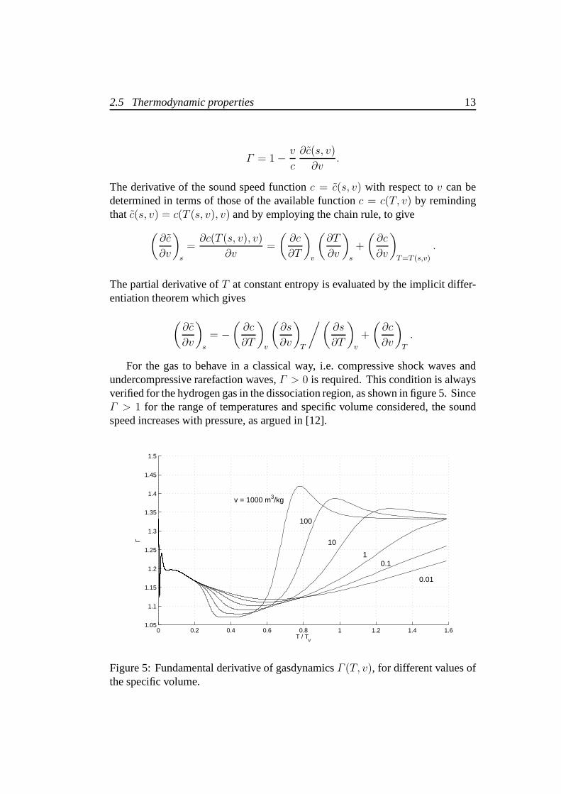
For the gas to behave in a classical way, i.e. compressive shock waves andundercompressive rarefaction waves,Γ > 0 is required. This condition is alwaysverified for the hydrogen gas in the dissociation region, as shown in figure 5. SinceΓ > 1 for the range of temperatures and specific volume considered, the soundspeed increases with pressure, as argued in [12].
0 0.2 0.4 0.6 0.8 1 1.2 1.4 1.61.05
1.1
1.15
1.2
1.25
1.3
1.35
1.4
1.45
1.5
T / Tv
Γ
v = 1000 m3/kg
100
10
10.1
0.01
Figure 5: Fundamental derivative of gasdynamicsΓ (T, v), for different values ofthe specific volume.

14 Chapter 2 Thermodynamics of hydrogen gas at equilibrium
3 Simplified hydrogen model
In this chapter a simplified thermodynamic model for a dissociating diatomic idealgas is described. Differently from chapter 2, rotations arenow taken as fully ex-cited and completely uncoupled from vibrations which are instead still representedthrough the Morse potential. Thus, equation (A.14) will be used to express the par-tition function of the hydrogen molecule H2, whereas for the atom H the expressionremains the same of the previous model (equation (A.16)).
Following the same steps of the previous chapter, we will derive expressionsfor the equations of state for energy, entropy and other relevant thermodynamicproperties of the gas. In order to underline the differencesresulting from differenttreatment of rotations, this simplified model will be compared with the previousone. A further comparison will be made with a chemical model (HC) of the mixtureH–H2 based on thelaw of mass action.
3.1 Dissociation equation and equilibrium properties
Dissociation equation
Using the stationarity of the Helmholtz free energy and the conservation of theatomic constituents of the gas leads to:
α2
1 − α=
√te−td/t
z(t)
v
vd≡ B(t, v), (3.1)
wherez(t) = e−De/kBTZv(T ) with Zv(T ) the vibrational partition function (A.10)and we have introduced the constant:
1
vd=
(g0H)2H5/2
2√
2 g0H2
Tr
√
Tv(2πkB)3/2u5/2
h3.
As a consequence, the dissociation coefficient is again uniquely determined by(3.1) as a function oft andv, so that at equilibriumα = α(t, v):
α(t, v) =1
2B(t, v)
[
√
1 + 4/B(t, v) − 1]
. (3.2)
15
16 Chapter 3 Simplified hydrogen model
Energy and entropy equations of state
Using the definitions of the internal energy (2.7) and entropy (2.9), the fundamentalrelation can be expressed in the parametric form:
ǫ(t, v) =1
2(5 + α)t+ (1 − α)[ǫv(t) − td],
σ(t, v) =1
2(5 + α)(1 + ln t) + (1 − α)σv(t)
+ (1 + α)
[
1 + ln
(
v
vd
)]
+ Υ (α) + σ0,
(3.3)
whereǫv(t) = x(t)/z(t) with x(t) = z′(t) t2 andσv(t) = x(t)t z(t)
+ln z(t) denote thecontributions to the internal energy and entropy due to vibrations, whileΥ (α) =−2α lnα− (1 − α) ln(1− α) is the contribution to the entropy due to the mixingof the molecular and atomic species andσ0 represents the entropy in a referencestate.
Pressure
The pressure function and its derivatives with respect tot andv are exactly thesame introduced in chapter 2 withα given by the equation (3.1).
Specific heats
Starting from their definitions we obtain, in adimensional form:
cv(t, v)
RH2
=1
2(5 + α) + (1 − α)ǫ′v(t) +
[
t
2− [ǫv(t) − td]
]
αt,
cP (t, v)
RH2
= cv(t, v) +(1 + α+ t αt)
2
1 + α− v αv.
(3.4)
Sound speed and fundamental derivative of gasdynamics
As for the pressure, the sound speed and the fundamental derivative of gasdynamicsare the same introduced in chapter 2, withα given by equation (3.1) andcv byequation (3.4).
3.2 Comparison between the models 17
3.2 Comparison between the models
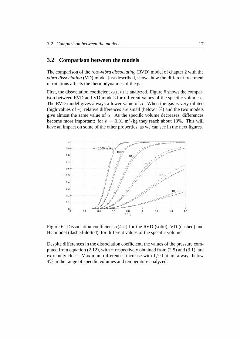
The comparison of theroto-vibra dissociating(RVD) model of chapter 2 with thevibra dissociating(VD) model just described, shows how the different treatmentof rotations affects the thermodynamics of the gas.
First, the dissociation coefficientα(t, v) is analyzed. Figure 6 shows the compar-ison between RVD and VD models for different values of the specific volumev.The RVD model gives always a lower value ofα. When the gas is very diluted(high values ofv), relative differences are small (below5%) and the two modelsgive almost the same value ofα. As the specific volume decreases, differencesbecome more important: forv = 0.01 m3/kg they reach about13%. This willhave an impact on some of the other properties, as we can see inthe next figures.
0 0.2 0.4 0.6 0.8 1 1.2 1.4 1.60
0.1
0.2
0.3
0.4
0.5
0.6
0.7
0.8
0.9
1
v = 1000 m3/kg100
10
1
0.1
0.01
T / Tv
α
Figure 6: Dissociation coefficientα(t, v) for the RVD (solid), VD (dashed) andHC model (dashed-dotted), for different values of the specific volume.
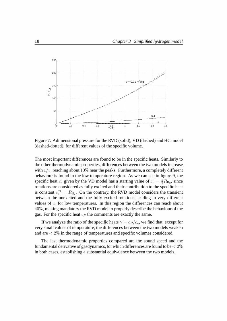
Despite differences in the dissociation coefficient, the values of the pressure com-puted from equation (2.12), withα respectively obtained from (2.5) and (3.1), areextremely close. Maximum differences increase with1/v but are always below4% in the range of specific volumes and temperature analyzed.
18 Chapter 3 Simplified hydrogen model
0 0.2 0.4 0.6 0.8 1 1.2 1.4 1.60
50
100
150
200
250
1
0.1
v = 0.01 m3/kg
T / Tv
P /
Pre
f
Figure 7: Adimensional pressure for the RVD (solid), VD (dashed) and HC model(dashed-dotted), for different values of the specific volume.
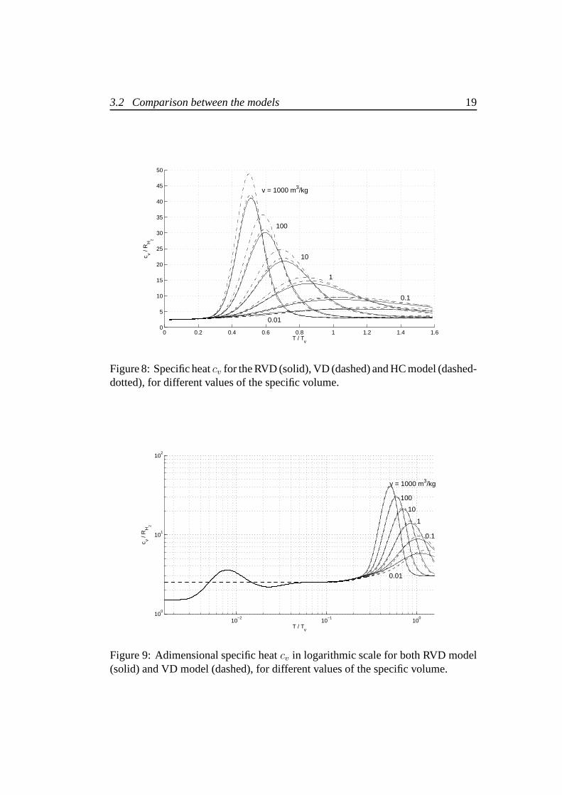
The most important differences are found to be in the specificheats. Similarly tothe other thermodynamic properties, differences between the two models increasewith 1/v, reaching about10% near the peaks. Furthermore, a completely differentbehaviour is found in the low temperature region. As we can see in figure 9, thespecific heatcv given by the VD model has a starting value ofcv = 5
2RH2
, sincerotations are considered as fully excited and their contribution to the specific heatis constantcrot
v = RH2. On the contrary, the RVD model considers the transient
between the unexcited and the fully excited rotations, leading to very differentvalues ofcv for low temperatures. In this region the differences can reach about40%, making mandatory the RVD model to properly describe the behaviour of thegas. For the specific heatcP the comments are exactly the same.
If we analyze the ratio of the specific heatsγ = cP/cv, we find that, except forvery small values of temperature, the differences between the two models weakenand are< 2% in the range of temperatures and specific volumes considered.
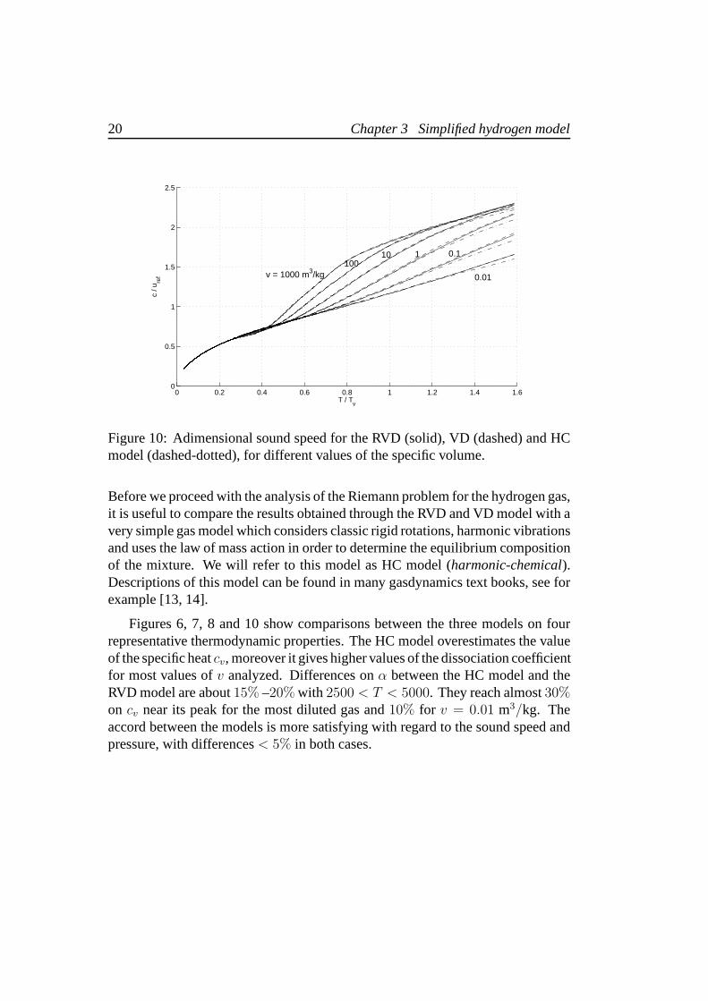
The last thermodynamic properties compared are the sound speed and thefundamental derivative of gasdynamics, for which differences are found to be< 2%in both cases, establishing a substantial equivalence between the two models.
3.2 Comparison between the models 19
0 0.2 0.4 0.6 0.8 1 1.2 1.4 1.60
5
10
15
20
25
30
35
40
45
50
v = 1000 m3/kg
100
10
1
0.1
0.01
T / Tv
c v / R
H2
Figure 8: Specific heatcv for the RVD (solid), VD (dashed) and HC model (dashed-dotted), for different values of the specific volume.
10−2
10−1
100
100
101
102
v = 1000 m3/kg
100
10
1
0.1
0.01
T / Tv
c v / R
H2
Figure 9: Adimensional specific heatcv in logarithmic scale for both RVD model(solid) and VD model (dashed), for different values of the specific volume.
20 Chapter 3 Simplified hydrogen model
0 0.2 0.4 0.6 0.8 1 1.2 1.4 1.60
0.5
1
1.5
2
2.5
v = 1000 m3/kg100
10 1 0.1
0.01
T / Tv
c / u
ref
Figure 10: Adimensional sound speed for the RVD (solid), VD (dashed) and HCmodel (dashed-dotted), for different values of the specificvolume.
Before we proceed with the analysis of the Riemann problem for the hydrogen gas,it is useful to compare the results obtained through the RVD and VD model with avery simple gas model which considers classic rigid rotations, harmonic vibrationsand uses the law of mass action in order to determine the equilibrium compositionof the mixture. We will refer to this model as HC model (harmonic-chemical).Descriptions of this model can be found in many gasdynamics text books, see forexample [13, 14].
Figures 6, 7, 8 and 10 show comparisons between the three models on fourrepresentative thermodynamic properties. The HC model overestimates the valueof the specific heatcv, moreover it gives higher values of the dissociation coefficientfor most values ofv analyzed. Differences onα between the HC model and theRVD model are about15% –20% with 2500 < T < 5000. They reach almost30%on cv near its peak for the most diluted gas and10% for v = 0.01 m3/kg. Theaccord between the models is more satisfying with regard to the sound speed andpressure, with differences< 5% in both cases.

4 Riemann problem for dissociating gas
In this chapter the Riemann problem of gasdynamics will be analyzed. It is aninitial value problem for the system of Euler equations withparticular initial con-ditions. The variables are characterized by a jump in their initial values, and areuniform on the left side and on the right side of a discontinuity; the two differentstates will be referred to as theleft stateand theright state. Since there is noreference length in the problem statement, the solution is self similar, namely it isconstant along any ray of thex-t plane. In general the solution consists of threewaves:shockor rarefaction wavesandcontact discontinuity, possibly of vanishingintensity. The intermediate wave is always a contact discontinuity while each ofthe two external waves can be either a shock or a rarefaction wave depending on theinitial conditions. The solution of the Riemann problem is very important in thesimulation of compressible flows since the Riemann problem is the starting pointto formulatefinite volume methodswhere it is solved at every interface betweentwo grid cells and at every time level.
Following Quartapelle et al. [4], we will first analyze the eigenstructure of theEuler equations which leads to the determination of the mathematical and physicalnature of the three different waves. Then a suitable formulation of the equationswhich describe the shock and the rarefaction wave for the case of the dissociatinggas will be introduced and the solution technique will be presented.
4.1 Eigenstructure of Euler equations
The Riemann problem of gasdynamics is formulated starting from the Euler equa-tions written in quasi-linear form and with the energy balance equation replacedby the entropy transport equation under the assumption thatany dissipative phe-nomena can be disregarded. The resulting system of hyperbolic equations ofgasdynamics assumes the form:
∂w
∂t+ A(w)
∂w
∂x= 0
with vectorw and matrixA(w) defined as follows:
w =
v
u
s
and A(w) =
u −v 0
v
(
∂P
∂v
)
s
u v
(
∂P
∂s
)
v
0 0 u
.
21
22 Chapter 4 Riemann problem for dissociating gas
Here v denotes the specific volume,u the velocity,s the specific entropy andP = P (s, v) is the pressure equation of state of the gas considered. The eigenvaluesof A(w) represent the speed at which information travels in the fluidand are theeigenvalues of the characteristic equation:
|A(w) − λ(w)I| = 0.
which gives:
λ1(w) = u− c(s, v), λ2(w) = u, λ3(w) = u+ c(s, v),
with c(s, v) = [∂P (s, ρ)/∂ρ]1/2 denoting the sound speed of the fluid. Theseeigenvalues are indipendent from the choice of the variables used to formulate theEuler system: using for example the densityρ instead of the specific volumevwould have led to exactly the same values ofλi.
To understand the nonlinear nature of the Euler system we have to computethe eigenvectors associated with the three eigenvalues. The eigenvectors are easilyfound to be:
r1(w) =
v
c(s, v)
0
, r2(w) =
−(
∂P∂s
)
v
0(
∂P∂v
)
s
, r3(w) =
v
−c(s, v)
0
.
4.2 Linear degeneracy and genuine nonlinearity
Every eigenvalueλi(w) defines a scalar field in the space of vectorsw = (v, u, s)T
and every eigenvectorri(w) defines a vector field in the same three-dimensionalspace. At the same time, the gradient of the eigenvalue∇
wλi(w) defines an-
other vector field. The linear or nonlinear nature of the waveassociated to eacheigenvalue depends on a simple geometrical relationship between the field of theeigenvector and that of the gradient of the corresponding eigenvalue, expressedby the scalar productr(w) · ∇
wλ(w). If this product never vanishes, then the
eigenvalue is said to begenuinely nonlinearwhile if it is always zero than theeigenvalue islinearly degenerate. For the Euler equations we can observe thatthe second eigenvalue is always linearly degenerate and that the first and thirdeigenvalues are found to be such that:
r1(w) · ∇wλ1(w) = cΓ and r3(w) · ∇
wλ3(w) = −cΓ,
whereΓ is the fundamental derivative of gasdynamics. As already shown inchapter 2, the functionΓ never vanishes for the gas considered here.

4.3 Contact discontinuity 23
4.3 Contact discontinuity
We first analyze the contact discontinuity. Let us consider awave travelling at aspeed given by the second eigenvalue of the Euler equations and determine thechange of the variables inside such a wave. This means to find the vector functionw = w(q) solution to the ordinary differential system:
dw
dq= α(q) r2(w),
with q a parameter which represents the indipendent variable andα(q) an arbitraryfunction whose choice fixes a parameterization of the solution. In terms of thecomponents ofr2(w), we have:
dv
dq= −α(q)
∂P (s, v)
∂s,
du
dq= 0,
ds
dq= α(q)
∂P (s, v)
∂v.
So, the velocity is constant through the contact discontinuity. Moreover, the ratioof the first and third equations gives
dv
ds= −∂P (s, v)
∂s
/
∂P (s, v)
∂v.
Let us now define a function of three independent variables:
Φ(s, v, P ) ≡ P (s, v) − P,
so that the equationΦ(s, v, P ) = 0 implicitly defines a functionv = v(s, P ). Thederivative ofv(s, P ) with respect to entropy is obtained by means of the theoremof partial derivation of the implicit functions:
(
∂v
∂s
)
P
= −∂Φ(s, v, P )
∂s∂Φ(s, v, P )
∂v
= −∂P (s, v)
∂s∂P (s, v)
∂v
.
Since this expression coincides withdv/ds along the contact discontinuity, thepressure is constant along the wave considered, whereasv and any other thermo-dynamic variable different from pressure can experience a jump in its values.
To summarize, the characteristic of the contact discontinuity is the constancy ofboth velocity and pressure; as we will see, these conditionswill be used to formulatethe Riemann problem as a system of two nonlinear equations with unknowns thevalues of the temperature on both sides of the wave.
24 Chapter 4 Riemann problem for dissociating gas
4.4 Rarefaction wave
We now analyze the rarefaction wave. Let us consider a wave linking a giveninitial state(vi, ui, si)
T with the states belonging to theintegral curves, which areby definition the curves tangent in every point to the direction of agiven eigenvector.In other words, an integral curve is the solution of the ordinary differential equationssystem
dw
dq= α(q) r1|3(w),
with initial conditionw(0) = wi = (vi, ui, si)T. For genuinely nonlinear eigen-
vectors, it is possible to use the eigenvalue as the parameter q = ξ = λ1|3(w(ξ))of the curve. The derivative of this relation with respect toξ gives α(ξ) =±1/[c(s, v)Γ (s, v)]. The system becomes:
dw
dξ=
±r1|3(w)
c(s, v)Γ (s, v), (4.1)
and must be solved with the initial conditionw(ξi) = wi, with ξi = λ1|3(wi).Substituting the expression ofr1|3(w), the equation of the third component of(4.1) says that the rarefaction wave is isentropic.
Reminding the thermodynamic models introduced in chapters2 and 3, we canwrite in dimensionless form:
σf(t, v, α(t, v)) = σi,
whereσi = σf(ti, vi, αi) andαi the solution ofα2i + β(ti, vi)(αi − 1) = 0. The
determination of the isentropic trasformation of the gas with specific entropyσi
requires to solve a nonlinear system of two equations:
φ(t, v, α, σi) = σf(t, v, α) − σi = 0
ψ(t, v, α) = α2 + β(t, v)(α− 1) = 0(4.2)
which, for any fixedt, gives the solutionv = vrar(t, σi) andα = αrar(t, σi) alongthe isentrope passing through(ti, vi). Thus, the solution of the rarefaction wavefor the case of the dissociating gas is more complicated thanfor the polytropicideal gas and requires the solution of the system (4.2) by means of the Newtonmethod. The pressure is provided immediately by the equation of state:
P rar(T ; i) = P (T, vrar(T, σi)).
The system (4.1) is reduced to only two equations and it is possible to obtain a directrelationship between velocity and specific volume by takingthe ratio between the
4.5 Shock wave 25
two first equations. The first order differential equation isseparable and can beintegrated to obtain:
urar1|3(v; i) = ui ±
∫ v
vi
c(si, v′)
v′dv′.
As we have seen in the description of the thermodynamics of the dissociatinghydrogen gas, the most convenient independent variable used to define all theother properties is the temperature. So, takenT as the independent variable, wehave:
P rar(T ; i) = P (si, T ),
urar1|3(T ; i) = ui ±
∫ T
Ti
c(si, T′)
vrar(T ′; i)
dvrar(T ′; i)
dT ′dT ′.
(4.3)
The derivativedvrar/dT can be evaluated by using the differentiation rule for im-plicit functions:
dvrar
dT= −
∂(φ, ψ)
∂(T, α)
∂(φ, ψ)
∂(v, α)
= −∂φ
∂T
∂ψ
∂α− ∂φ
∂α
∂ψ
∂T∂φ
∂v
∂ψ
∂α− ∂φ
∂α
∂ψ
∂v
. (4.4)
Finally, we must notice that, when the solution of the Riemann problem consistsof two rarefaction waves, for particular values of the initial velocities it is possiblethe formation of a region of vacuum behind the wave’s tails. This circumstanceis identified by the vanishing of the temperature on the contact discontinuity. Wecan define a relative velocityνvacuum:
νvacuum= −∫ Tℓ
0
c(sℓ, T )
vrar(T ; l)
dvrar(T ; l)
dTdT −
∫ Tr
0
c(sr, T )
vrar(T ; r)
dvrar(T ; r)
dTdT (4.5)
such that, forνrℓ = ur − uℓ ≥ νvacuum, a region of vacuum occurs.
4.5 Shock wave
In this section the solution of the shock wave is obtained. Ingeneral the shockmoves with a speedσ 6= 0 with respect to the system of reference in whichthe Riemann problem is defined. The solution is achieved using the Rankine–Hugoniot jump conditionsf(w) − f(wi) = σ[w − wi], with f(w) the flux ofthe hyperbolic system in the conservative form andw = (ρ,m = ρu, Et)T. It
26 Chapter 4 Riemann problem for dissociating gas
is convenient to move to the frame of reference of the shock inwhich the fluidvelocity isU = u − σ, so that a steady-state version of the Rankine–Hugoniotconditions is obtained, namely:
Ui/vi = U/v,
U2i
/
vi + Pi = U2/
v + P,
12U2
i + ei + Pivi = 12U2 + e+ Pv.
Combining the three equations leads to the purely thermodynamic relation:
e(P, v) − ei + 12(Pi + P )(v − vi) = 0,
which definesP = PRH(v; i) implicitly.
Using the definition of themass velocityJ =u− ui
v − vi, it is possible to obtain
the expression of the velocity behind the shock
uRH1|3(v; i) = ui ∓
√
−[
PRH(v; i) − Pi
]
(v − vi)
in which the subscript1|3 refers to the first and third eigenvalue of the Euler equa-tions and the signs∓ are determined by the propertyΓ > 0 which guarantees thatthe wave is compressive.
Similarly to the rarefaction wave, it is convenient to formulate the solution of theshock wave in terms of the temperature. Reminding the thermodynamic relationsof the dissociating gas, the Rankine–Hugoniot equation becomes, in dimensionlessform:
ǫf(t, α) − ǫi + 12
[
pi + pf(t, v, α)]
(v − vi) = 0,
wereǫi = ǫf(ti, αi),pi = pf(ti, vi, αi) andαi the solution ofα2i +β(ti, vi)(αi−1) =
0. The determination of the solution of the shock wave requires to solve a nonlinearsystem of two equations:
φ(t, v, α, σi) = ǫf(t, α) − ǫi + 12
[
pi + pf(t, v, α)]
(v − vi) = 0,
ψ(t, v, α) = α2 + β(t, v)(α− 1) = 0,(4.6)
which, for any fixedt, gives the solutionvRH = v(t; i) andα = α(t; i) behind theshock. The pressure is provided immediately by the equationof state:
PRH(T ; i) = P (T, vRH(T ; i)). (4.7)
4.6 Structure of the Riemann problem 27
Now the velocity after the shock wave is easily expressed in the form
uRH1|3(T ; i) = ui ∓
√
−[
PRH(T ; i) − Pi
][
vRH(T ; i) − vi
]
. (4.8)
The derivativedvRH/dT can be evaluated by using the differentiation rule forimplicit functions:
dvRH
dT= −
∂φ
∂T
∂ψ
∂α− ∂φ
∂α
∂ψ
∂T∂φ
∂v
∂ψ
∂α− ∂φ
∂α
∂ψ
∂v
. (4.9)
4.6 Structure of the Riemann problem
Finally, the characteristics of the contact discontinuitydescribed in section 4.3 canbe exploited to formulate the equations representing the Riemann problem.
We will denote byu1(T ; l) andP (T ; l) respectively the velocity and the pres-sure after the wave which connects the left statel = (Tℓ, Pℓ, uℓ)
T with a genericstate characterized by a temperatureT . The analytical form of the two functionsu = u1(T ; l) andP = P (T ; l) depends on the nature of the wave that can beeither a shock wave (T > Tℓ) or a rarefaction wave (T < Tℓ). Similarly,u3(T ; r)andP (T ; r) denote respectively the velocity and the pressure after thewave whichconnects the right stater = (Tr, Pr, ur)
T with a generic state characterized by atemperatureT . We can summarize the form ofu1(T ; l) andu3(T ; r) as follows:
u1(v; l) ≡
urar1 (T ; l) if T < Tℓ
uRH1 (T ; l) if T > Tℓ
and u3(v; r) ≡
urar3 (T ; r) if T < Tr
uRH3 (T ; r) if T > Tr
with the superscriptsrar andRH denoting the solution of the rarefaction wave orthe shock wave given by equations (4.3) and (4.8). As alreadyseen, the functionsdefining the velocities depend on the eigenvalues1 and3. Conversely, the functionsdefining the pressure are indipendent from the eigenvalue and are:
P (v; l) ≡
P rar(v; l) if T < Tℓ
PRH(v; l) if T > Tℓ
and P (v; r) ≡
P rar(v; r) if T < Tr
PRH(v; r) if T > Tr
with P rar andPRH given by equations (4.3) and (4.7) respectively. To solve theRiemann problem requires to determine the valuesT ⋆
ℓ , T ⋆r , P ⋆ andu⋆ which char-
acterize the states on the two sides of the contact discontinuity. To simplify thenotation we will refer to the two unknowns asT ≡ T ⋆
ℓ andW ≡ T ⋆r . To guarantee
28 Chapter 4 Riemann problem for dissociating gas
the property of equality of the values of velocity and pressure on the two sides ofthe contact discontinuity,T andW must be the solutions of the nonlinear systemof two equations:
{
u1(T ; l) = u3(W ; r),
P (T ; l) = P (W ; r),
which can be written also as:{
φ(ℓ,r)(T,W ) = 0,
ψ(ℓ,r)(T,W ) = 0,
whereφ(ℓ,r)(T,W ) = u1(T ; l)−u3(W ; r) andψ(ℓ,r)(T,W ) = P (T ; l)−P (W ; r).This system can be solved numerically with a Newton method, which needs toevaluate the Jacobian matrix:
∂(φ(ℓ,r), ψ(ℓ,r))
∂(T,W )≡
du1(T ; l)
dT−du3(W ; r)
dW
dP (T ; l)
dT−dP (W ; r)
dW
. (4.10)
For the case of the gas considered2, the expressions of the elements of the Jacobianmatrix, when the wave is a rarefaction wave, are the following:
durar1|3(T ; i)
dT= ± c(si, T )
vrar(T ; i)dvrar(T ; i)
dT
and
dP rar(T ; i)dT
=dP (T, vrar(T ; i))
dT=∂P (T, v)
∂T+∂P (T, v)
∂v
dvrar(T ; i)dT
.
The derivativedvrar(T ; i)/dT is given by equation (4.4). On the other hand, whenthe wave is a shock wave, the derivatives are:
dPRH(T ; i)dT
=dP (T, vRH(T ; i))
dT=∂P (T, v)
∂T+∂P (T, v)
∂v
dvRH(T ; i)dT
and
duRH1|3(T ; i)
dT= ±
dPRH(T ; i)dT
[
vRH(T ; i) − vi
]
+dvRH(T ; i)
dT
[
PRH(T ; i) − Pi
]
2√
−[PRH(T ; i) − Pi][vRH(T ; i) − vi],
2As well as for any mixture of nonpolytropic gases.

4.6 Structure of the Riemann problem 29
wheredvRH(T ; i)/dT is given by equation (4.9).
The existence and uniqueness of the solution of the Riemann problem can bedemonstrated under the assumption that∂e(P, v)/∂v > 0. In this case the Newtonmethod will converge to the solution provided the initial guess is close enough tothe solution: taking the initial guess as the arithmetic mean of the two initial valuesTℓ andTr is simple and turns out to be also effective.

30 Chapter 4 Riemann problem for dissociating gas

5 Results
In this chapter the Hugoniot curves for the hydrogen gas are first analyzed to high-light the consequences of the dissociation. Then, results of some Riemann problemin the presence of dissociation and in the low temperature region are presented anddiscussed. Three different kinds of solutions are considered: symmetrical solu-tions with either two rarefaction waves or two shock waves, and mixed solutionswith one rarefaction wave and one shock wave. A comparison between the resultsobtained by means of the RVD and VD models is made. Initial conditions for everyRiemann problem are suggested by the analysis of chapter 3, in order to underlinedifferences between the models for certain initial thermodynamic data, as well asto verify their equivalence for other initial data. Finally, for the case of the shockwaves, a comparison with results provided in [5] is made.
5.1 Hugoniot curves
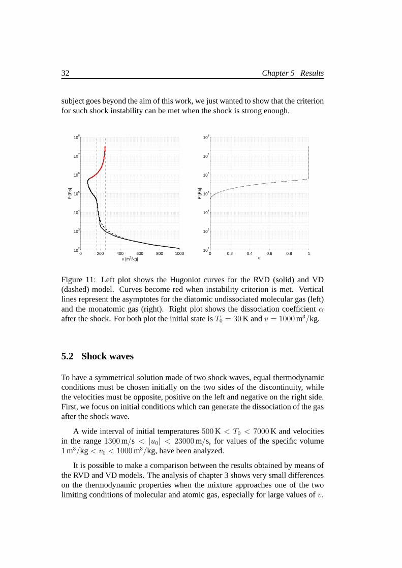
The Hugoniot curveor Hugoniot adiabatis fundamental in the study of shockwaves. It is the locus of all the thermodynamic states(v, P ) which may be con-nected by a single shock to an initial state(v0, P0).
Starting from a small value of pressure (and so of temperature), the Hugoniotcurve first tends to the vertical asymptote pertaining to thediatomic undissociatedideal gas. When pressure increases further, dissociation occurrs and makes thecurve cross the diatomic gas asymptote. Then, for higher pressures, the Hugoniotcurve reaches a minimum value ofv, after which the curve has an inversion whenthe dissociation is complete. Finally, the curve tends to the vertical asymptote of themonatomic gas, but from the left side instead of from the right. Figure 11 shows theadiabats for the RVD and VD model. They agree quite well, except for small valuesof the pressure after the shock. This will determine differences in the solution ofthe Riemann problem with two shock waves in the low temperature region. Thedissociation coefficientα after the shock increases with the shock strength becausethe increment in temperature prevails over the diminishingspecific volume.
Furthermore, referring to Bates and Montgomery [15], it is interesting to no-tice that, if the shock is strong enough, an exotic mechanismknown asacousticemissioncould manifests. This is a shock wave instability which doesnot implyan anomalous behaviour of the shock sinceΓ is always positive. It requires theslope of the Hugoniot curve to be within a critical range. Figure 11 confirms thisoccurrence for the hydrogen gas when the shock wave is such toconnect an initiallow temperature state to completely dissociated conditions. The analysis of thiskind of instability is very important in the study of the implosion ofinertial con-finement fusion of pellet materials, for which the hydrogen is used. However, this
31
32 Chapter 5 Results
subject goes beyond the aim of this work, we just wanted to show that the criterionfor such shock instability can be met when the shock is strongenough.
0 200 400 600 800 100010
2
103
104
105
106
107
108
v [m3/kg]
P [P
a]
0 0.2 0.4 0.6 0.8 110
2
103
104
105
106
107
108
α
P [P
a]
Figure 11: Left plot shows the Hugoniot curves for the RVD (solid) and VD(dashed) model. Curves become red when instability criterion is met. Verticallines represent the asymptotes for the diatomic undissociated molecular gas (left)and the monatomic gas (right). Right plot shows the dissociation coefficientαafter the shock. For both plot the initial state isT0 = 30 K andv = 1000 m3/kg.
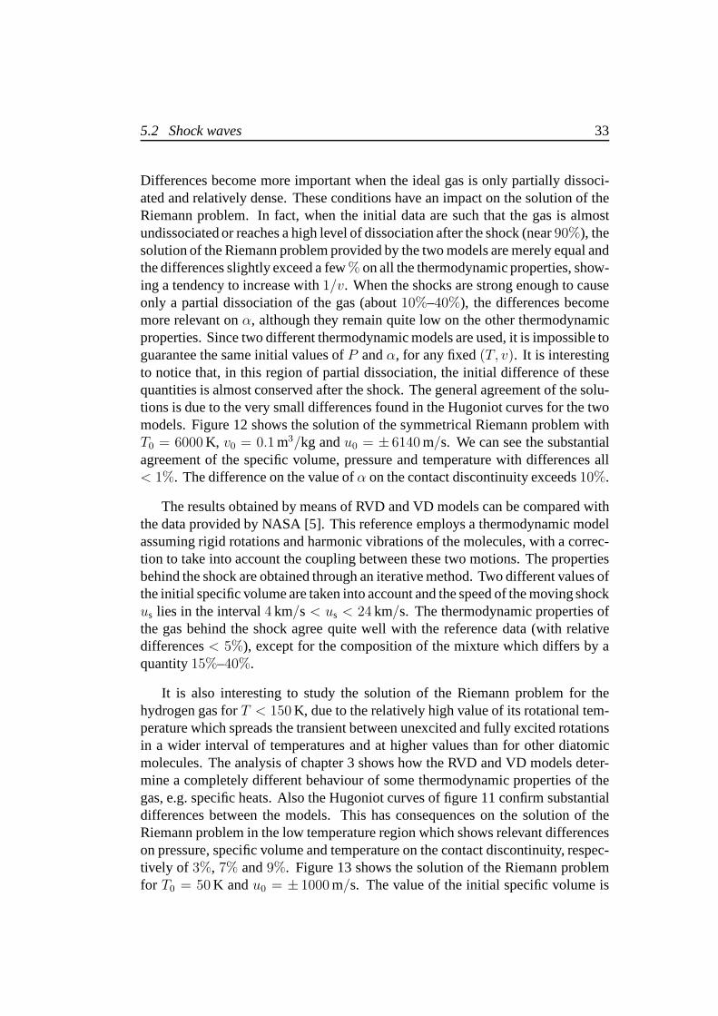
5.2 Shock waves
To have a symmetrical solution made of two shock waves, equalthermodynamicconditions must be chosen initially on the two sides of the discontinuity, whilethe velocities must be opposite, positive on the left and negative on the right side.First, we focus on initial conditions which can generate thedissociation of the gasafter the shock wave.
A wide interval of initial temperatures500 K < T0 < 7000 K and velocitiesin the range1300 m/s < |u0| < 23000 m/s, for values of the specific volume1 m3/kg< v0 < 1000 m3/kg, have been analyzed.
It is possible to make a comparison between the results obtained by means ofthe RVD and VD models. The analysis of chapter 3 shows very small differenceson the thermodynamic properties when the mixture approaches one of the twolimiting conditions of molecular and atomic gas, especially for large values ofv.
5.2 Shock waves 33
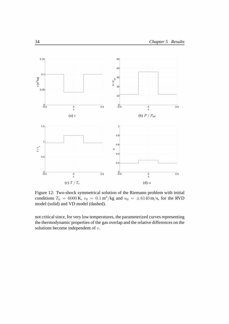
Differences become more important when the ideal gas is onlypartially dissoci-ated and relatively dense. These conditions have an impact on the solution of theRiemann problem. In fact, when the initial data are such thatthe gas is almostundissociated or reaches a high level of dissociation afterthe shock (near90%), thesolution of the Riemann problem provided by the two models are merely equal andthe differences slightly exceed a few% on all the thermodynamic properties, show-ing a tendency to increase with1/v. When the shocks are strong enough to causeonly a partial dissociation of the gas (about10%–40%), the differences becomemore relevant onα, although they remain quite low on the other thermodynamicproperties. Since two different thermodynamic models are used, it is impossible toguarantee the same initial values ofP andα, for any fixed(T, v). It is interestingto notice that, in this region of partial dissociation, the initial difference of thesequantities is almost conserved after the shock. The generalagreement of the solu-tions is due to the very small differences found in the Hugoniot curves for the twomodels. Figure 12 shows the solution of the symmetrical Riemann problem withT0 = 6000 K, v0 = 0.1 m3/kg andu0 = ± 6140 m/s. We can see the substantialagreement of the specific volume, pressure and temperature with differences all< 1%. The difference on the value ofα on the contact discontinuity exceeds10%.
The results obtained by means of RVD and VD models can be compared withthe data provided by NASA [5]. This reference employs a thermodynamic modelassuming rigid rotations and harmonic vibrations of the molecules, with a correc-tion to take into account the coupling between these two motions. The propertiesbehind the shock are obtained through an iterative method. Two different values ofthe initial specific volume are taken into account and the speed of the moving shockus lies in the interval4 km/s< us < 24 km/s. The thermodynamic properties ofthe gas behind the shock agree quite well with the reference data (with relativedifferences< 5%), except for the composition of the mixture which differs byaquantity15%–40%.
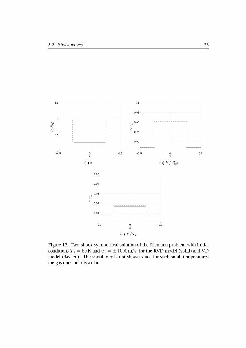
It is also interesting to study the solution of the Riemann problem for thehydrogen gas forT < 150 K, due to the relatively high value of its rotational tem-perature which spreads the transient between unexcited andfully excited rotationsin a wider interval of temperatures and at higher values thanfor other diatomicmolecules. The analysis of chapter 3 shows how the RVD and VD models deter-mine a completely different behaviour of some thermodynamic properties of thegas, e.g. specific heats. Also the Hugoniot curves of figure 11confirm substantialdifferences between the models. This has consequences on the solution of theRiemann problem in the low temperature region which shows relevant differenceson pressure, specific volume and temperature on the contact discontinuity, respec-tively of 3%, 7% and9%. Figure 13 shows the solution of the Riemann problemfor T0 = 50 K andu0 = ± 1000 m/s. The value of the initial specific volume is
34 Chapter 5 Results
−0.5 0 0.50
0.05
0.1
0.15
x
v [m
3 /kg]
(a)v
−0.5 0 0.50
10
20
30
40
50
x
P /
Pre
f(b) P / Pref
−0.5 0 0.50
0.5
1
1.5
x
T /
T v
(c) T / Tv
−0.5 0 0.50
0.2
0.4
0.6
0.8
1
x
α
(d) α
Figure 12: Two-shock symmetrical solution of the Riemann problem with initialconditionsT0 = 6000 K, v0 = 0.1 m3/kg andu0 = ± 6140 m/s, for the RVDmodel (solid) and VD model (dashed).
not critical since, for very low temperatures, the parameterized curves representingthe thermodynamic properties of the gas overlap and the relative differences on thesolutions become independent ofv.
5.2 Shock waves 35
−0.5 0 0.50
0.5
1
1.5
x
v [m
3 /kg]
(a)v
−0.5 0 0.50
0.02
0.04
0.06
0.08
0.1
x
P /
Pre
f
(b) P / Pref
−0.5 0 0.50
0.01
0.02
0.03
0.04
0.05
x
T /
T v
(c) T / Tv
Figure 13: Two-shock symmetrical solution of the Riemann problem with initialconditionsT0 = 50 K andu0 = ± 1000 m/s, for the RVD model (solid) and VDmodel (dashed). The variableα is not shown since for such small temperaturesthe gas does not dissociate.
36 Chapter 5 Results
5.3 Rarefaction waves
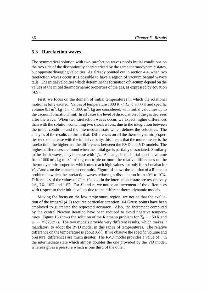
The symmetrical solution with two rarefaction waves needs initial conditions onthe two side of the discontinuity characterized by the same thermodynamic states,but opposite diverging velocities. As already pointed out in section 4.4, when tworarefaction waves occur it is possible to have a region of vacuum behind wave’stails. The initial velocities which determine the formation of vacuum depend on thevalues of the initial thermodynamic properties of the gas, as expressed by equation(4.5).
First, we focus on the domain of initial temperatures in which the rotationalmotion is fully excited. Values of temperature1000 K < T0 < 9000 K and specificvolume0.1 m3/kg< v < 1000 m3/kg are considered, with initial velocities up tothe vacuum formation limit. In all cases the level of dissociation of the gas decresesafter the wave. When two rarefaction waves occur, we expect higher differencesthan with the solution containing two shock waves, due to theintegration betweenthe initial condition and the intermediate state which defines the velocities. Theanalysis of the results confirms that. Differences on all thethermodynamic proper-ties tend to increase with the initial velocity, this means that the more intense is therarefaction, the higher are the differences between the RVDand VD models. Thehighest differences are found when the initial gas is partially dissociated. Similarlyto the shock waves, they increase with1/v. A change in the initial specific volumefrom 1000 m3/kg to 0.1 m3/kg can triple or more the relative differences on thethermodynamic properties which now reach high values not only for α but also forP ,T andv on the contact discontinuity. Figure 14 shows the solution of a Riemannproblem in which the rarefaction waves reduce gas dissociation from40% to 10%.Differences of the values ofT , v,P andα in the intermediate state are respectively2%, 7%, 10% and14%. ForP andα, we notice an increment of the differenceswith respect to their initial values due to the different thermodynamic models.
Moving the focus on the low temperature region, we notice that the evalua-tion of the integral (4.3) requires particular attention:64 Gauss points have beenemployed to guarantee the requested accuracy. Also, the increment computedby the central Newton iteration have been reduced to avoid negative tempera-tures. Figure 15 shows the solution of the Riemann problem for T0 = 150 K andu0 = ∓ 820 m/s. The two models provide very different results, which makes itmandatory to adopt the RVD model in this range of temperatures. The relativedifference on the temperature is about35%. If we observe the specific volume andpressure, differences are much greater. The RVD model provides a value ofv inthe intermediate state which almost doubles the one provided by the VD model,whereas gives a pressure which is one third of the other.
5.3 Rarefaction waves 37
−0.5 0 0.50
1
2
3
4
5
6
7
8
x
v [m
3 /kg]
(a)v
−0.5 0 0.50
2
4
6
8
10
12
14
16
18
x
P /
Pre
f
(b) P / Pref
−0.5 0 0.50
0.5
1
1.5
x
T /
T v
(c) T / Tv
−0.5 0 0.50
0.2
0.4
0.6
0.8
1
x
α
(d) α
Figure 14: Two-rarefaction symmetrical solution of the Riemann problem withinitial conditionsT0 = 7500 K, u0 = ∓ 23000 m/s andv = 0.1 m3/kg, for theRVD model (solid) and VD model (dashed). The choice ofu0 is such that the gascan encompass the most critical values ofα.

38 Chapter 5 Results
−0.5 0 0.50
0.5
1
1.5
x
v [m
3 /kg]
(a)v
−0.5 0 0.50
0.05
0.1
0.15
0.2
0.25
0.3
x
P /
Pre
f
(b) P / Pref
−0.5 0 0.50
0.005
0.01
0.015
0.02
0.025
0.03
x
T /
T v
(c) T / Tv
Figure 15: Two-rarefaction symmetrical solution of the Riemann problem withinitial conditionsT0 = 150 K, u0 = ∓ 820 m/s andv = 0.1 m3/kg, for the RVDmodel (solid) and VD model (dashed).
5.4 Mixed solution 39
5.4 Mixed solution
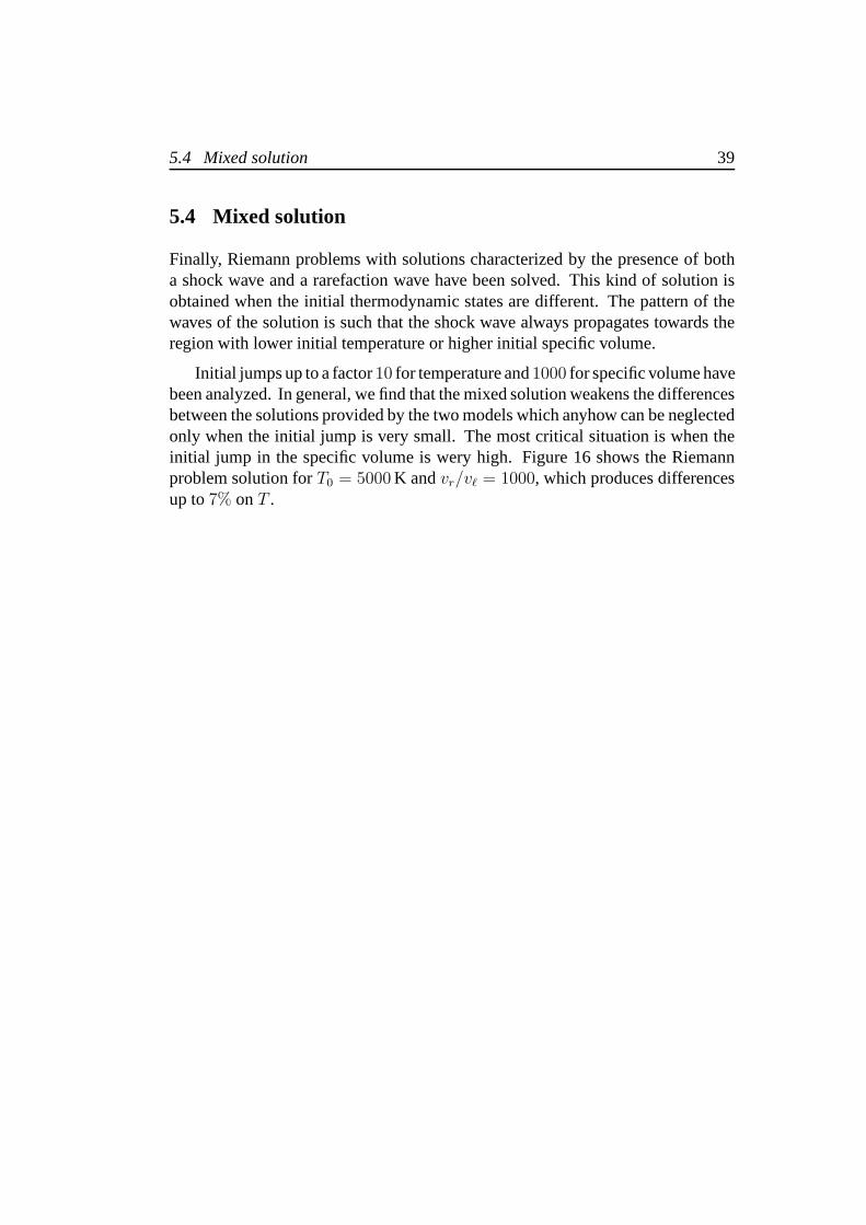
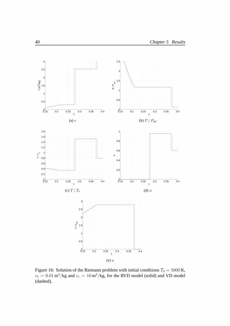
Finally, Riemann problems with solutions characterized bythe presence of botha shock wave and a rarefaction wave have been solved. This kind of solution isobtained when the initial thermodynamic states are different. The pattern of thewaves of the solution is such that the shock wave always propagates towards theregion with lower initial temperature or higher initial specific volume.
Initial jumps up to a factor10 for temperature and1000 for specific volume havebeen analyzed. In general, we find that the mixed solution weakens the differencesbetween the solutions provided by the two models which anyhow can be neglectedonly when the initial jump is very small. The most critical situation is when theinitial jump in the specific volume is wery high. Figure 16 shows the Riemannproblem solution forT0 = 5000 K andvr/vℓ = 1000, which produces differencesup to7% onT .
40 Chapter 5 Results
0.15 0.2 0.25 0.3 0.35 0.40
0.5
1
1.5
2
2.5
3
x
v [m
3 /kg]
(a)v
0.15 0.2 0.25 0.3 0.35 0.40
0.5
1
1.5
2
2.5
xP
/ P
ref
(b) P / Pref
0.15 0.2 0.25 0.3 0.35 0.40
0.2
0.4
0.6
0.8
1
1.2
1.4
1.6
1.8
x
T /
T v
(c) T / Tv
0.15 0.2 0.25 0.3 0.35 0.40
0.2
0.4
0.6
0.8
1
x
α
(d) α
0.15 0.2 0.25 0.3 0.35 0.40
0.5
1
1.5
2
2.5
3
x
u / u
ref
(e)u
Figure 16: Solution of the Riemann problem with initial conditionsT0 = 5000 K,vℓ = 0.01 m3/kg andvr = 10 m3/kg, for the RVD model (solid) and VD model(dashed).
6 Conclusions
This work conducted a comparison between a completely consistent thermody-namic model (RVD) and two simplified ones (VD and HC) for a mixture consist-ing of a diatomic molecular gas that can dissociate into atomic constituents. Thecomplete model differs from the others on the treatment of molecular rotations andvibrations, which are completely coupled. The hydrogen gashave been analyzed,because of the high value of its rotational temperature. Thethermodynamic prop-erties provided by the complete model have been compared with [9] to verify theiraccuracy in the low temperature domain in which it gives a completely differentdescription with respect to the simplified models. Also important differences havebeen found when the gas is only partially dissociated (up toα ≃ 0.4), this isemphasized for small values of the specific volume.temperature to
Then, starting from Quartapelle et al. [4], a new formulation of the Riemannproblem of gasdynamics for the dissociating gas has been introduced. The pres-ence of the dissociation requires to solve an additional nonlinear problem to havethe solution of either the rarefaction wave or the shock wave, which is now com-putationally more expensive. The Riemann problem has been analyzed for thegas models considered from very small values of the temperature up to completedissociation and the results obtained by means of the RVD andVD models havebeen compared. Results for values of temperature for which the rotational motionof the molecule is fully excited, i.e.T > 300 K, have been considered. Reflectingthe initial thermodynamic comparison, the most important differences have beenfound when the gas is only partially dissociated after the shock or the rarefactionwave. In this case, the choice of the complete model is mandatory to have the cor-rect solution. The analysis of the low temperature region underlines the importanceof choosing the complete model which guarantees the correctdescription of theroto-vibrational molecular motion. For very small temperatures, the RVD and VDmodels can provide completely different results, especially when two rarefactionwaves occur.
Future work should be directed on the confirmation of the numerical resultsby shock tube experiments as well as on the improvement of thecomputationalefficiency of the solution by a Roe’s linearization [16] of the Riemann problem forthe dissociating gas to be introduced in the numerical solution schemes by finitevolumes. Further work could be aimed at extending the thermodynamic modelin order to have a description of an air model valid for hypersonic aerodynamicstudies. The application of a H2 model which allows ionization possibly in thecontext of relativistic flows represents also a challenge worth of being accepted.
41

42 Chapter 6 Conclusions
A Partition functions for molecular and atomic hy-drogen
In this appendix the partition functions used to derive the properties of both molec-ular and atomic hydrogen are introduced. In general the partition function is ex-pressed by:
Z(β, V, N) =∑
j
e−Ejβ , (A.1)
whereβ = 1/(kBT ) with kB = 1.38065 × 10⁻²³ J/K denoting the Boltzmannconstant,N the number of the particles contained in the volumeV andEj thetotal energy of the whole system in the microscopic statej, the summation beingextended to all of the possible states of the system. When a system is composed ofnoninteracting material particles, such as the molecules of an ideal gas, the energyof the system is the sum over the energies of all of its particles. As a consequence,the partition function can be factorized in elementary partition functions of theconstituent elements. In particular, for a system ofN indistinguishable identicalparticles, the partition function becomesZ(β, V, N) = [Z(β, V )]N/N !, whereZ(β, V ) is the partition function of a single molecule.
The energy levels of each single molecule are the eigenvalues of the timeindependent Schrödinger equation for the whole molecule:
Hψ = Eψ, (A.2)
in which ψ is the wavefunction andH denotes the hamiltonian operator whichcomprises the total energy of the molecule.
Assuming that the energy of the particle has independent additive contributions,the partition function of the single molecule will assume the factorized form:
Z(β, V ) =∏
m
Zm(β, V ) (A.3)
In the following, we will give the expression of the partition function of eachcontribution used express the partition function of the whole molecule H2 and atomH.
43
44 Appendix A Partition functions for molecular and atomic hydrogen
A.1 The hydrogen molecule
A.1.1 Translation
As is well known3, the translational partition function of a free particle is:
Ztr(T, V ) =
(
2πmkBT
h2
)3/2
V, (A.4)
wherem denotes the mass of the particle andh = 6.626068 × 10⁻³⁴ m2 kg/s thePlanck constant.
A.1.2 Rotation
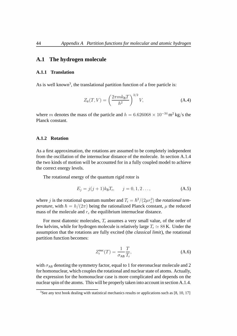
As a first approximation, the rotations are assumed to be completely independentfrom the oscillation of the internuclear distance of the molecule. In section A.1.4the two kinds of motion will be accounted for in a fully coupled model to achievethe correct energy levels.
The rotational energy of the quantum rigid rotor is
Ej = j(j + 1)kBTr, j = 0, 1, 2 . . . , (A.5)
wherej is the rotational quantum number andTr = ~2/(2µr2
e) therotational tem-perature, with ~ = h/(2π) being the rationalized Planck constant,µ the reducedmass of the molecule andre the equilibrium internuclear distance.
For most diatomic molecules,Tr assumes a very small value, of the order offew kelvins, while for hydrogen molecule is relatively largeTr ≃ 88 K. Under theassumption that the rotations are fully excited (theclassical limit), the rotationalpartition function becomes:
Znucr (T ) =
1
σAB
T
Tr, (A.6)
with σAB denoting the symmetry factor, equal to 1 for eteronuclear molecule and 2for homonuclear, which couples the rotational and nuclear state of atoms. Actually,the expression for the homonuclear case is more complicatedand depends on thenuclear spin of the atoms. This will be properly taken into account in section A.1.4.
3See any text book dealing with statistical mechanics results or applications such as [8, 10, 17]
A.1 The hydrogen molecule 45
A.1.3 Vibration
The simplest way to describe the vibrational motion of a diatomic molecule isusing the harmonic oscillator model whose potential isV (r) = 1
2k(r − re)
2, withk denoting the elastic constant andr the distance between atomic nuclei. A closedform solution for the vibrational eigenvalues can be achieved:
En =
(
n+1
2
)
~ω0, n = 0, 1, 2 . . . , (A.7)
with ω0 =√
k/µ , which are a uniform infinite ladder with separation~ω0.This model is satisfactory just for small deviations from equilibrium bond length,whereas for larger oscillations the parabolic approximation of the potential must beabandoned. TheMorse potential, introduced in [3], provides a much more realisticdescription of molecular potential:
V (r) = De
[
(
1 − e−(r−re)/λ)2 − 1
]
, for r > 0, (A.8)
whereDe is the potential minimum depth,r− re the displacement from the equi-librium distancere andλ is a length scale of the Morse potential curve. The threeparameters depend on the molecule. The Schrödinger equation with the Morsepotential can be solved analytically and leads to the eigenvalues:
En = −De+De
[
2 −(
n+1
2
)
χe
](
n +1
2
)
χe, n = 0, 1, 2 . . . , nmax, (A.9)
whereχe = ~/(λ√
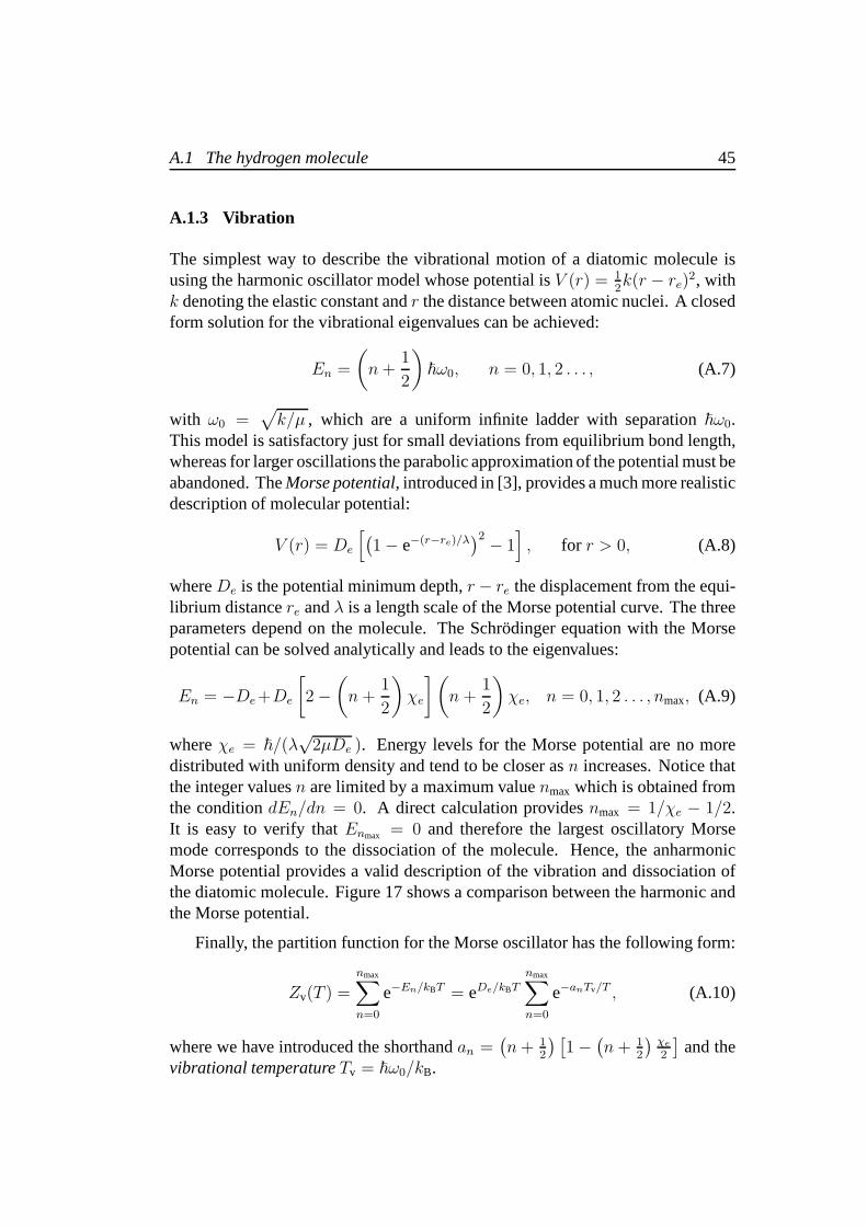
2µDe ). Energy levels for the Morse potential are no moredistributed with uniform density and tend to be closer asn increases. Notice thatthe integer valuesn are limited by a maximum valuenmax which is obtained fromthe conditiondEn/dn = 0. A direct calculation providesnmax = 1/χe − 1/2.It is easy to verify thatEnmax = 0 and therefore the largest oscillatory Morsemode corresponds to the dissociation of the molecule. Hence, the anharmonicMorse potential provides a valid description of the vibration and dissociation ofthe diatomic molecule. Figure 17 shows a comparison betweenthe harmonic andthe Morse potential.
Finally, the partition function for the Morse oscillator has the following form:
Zv(T ) =
nmax∑
n=0
e−En/kBT = eDe/kBTnmax∑
n=0
e−anTv/T , (A.10)
where we have introduced the shorthandan =(
n+ 12
) [
1 −(
n+ 12
)
χe
2
]
and thevibrational temperatureTv = ~ω0/kB.
46 Appendix A Partition functions for molecular and atomic hydrogen
0 0.5 1 1.5 2 2.5 3 3.5 4 4.5 5−1.5
−1
−0.5
0
0.5
r / re
V /
De
and
En /
De
n = 0n = 1
n = 2
n = 3
n = 0n = 1
n = 2n = 3
Figure 17: Potential curves and energy levels for the harmonic (red dashed) andMorse (black solid) oscillators.
A.1.4 Roto-vibration
Till now rotational and vibrational degrees of freedom havebeen considered ascompletely independent. Overcoming this assumption is mandatory for hydrogenmolecule due to the relatively high value of its rotational temperature.
The Schrödinger equation for rotational and vibrational anharmonic motionmust be solved. No closed form solution exists, but many approximation tech-niques4 can give mathematical expressions of the eigenvaluesEn,j which nowdepend on both rotational and vibrational quantum numbers.The most usefulexpression of theroto-vibrationaleigenvalues is the one presented by Harris andBertolucci [22]:
En,j
De= +
[
1 − j(j + 1)(κ2χe)2]
j(j + 1)(κχe)2
− 1 +[
2 −(
n+ 12
)
χe
] (
n + 12
)
χe
− 3j(j + 1)(
n+ 12
)
(1 − κ)(κχe)3,
(A.11)
whereκ = λ/re, which combines good accuracy and easy usage for our aim.
4Some examples can be found in [18, 19, 20, 21].
A.1 The hydrogen molecule 47
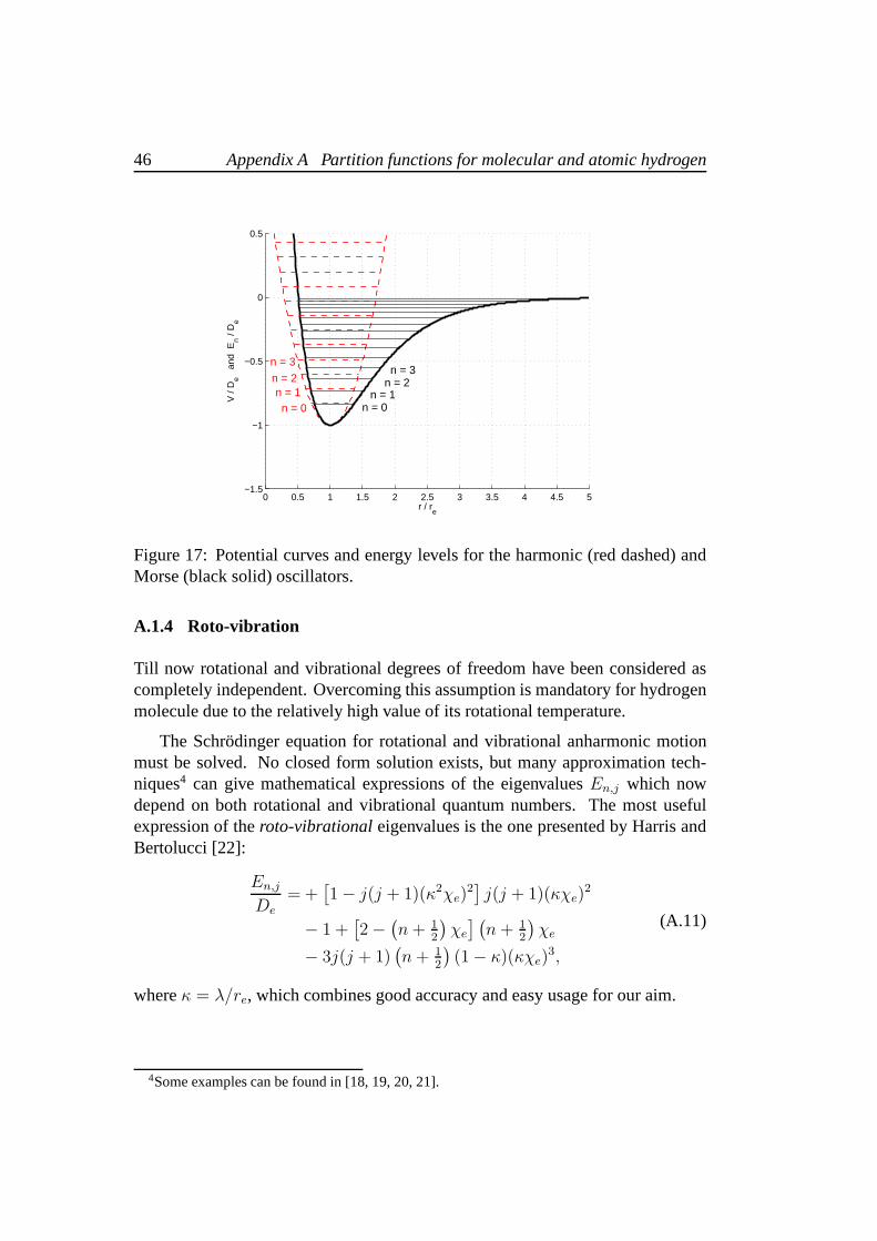
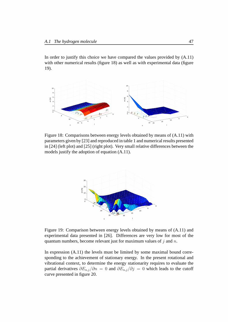
In order to justify this choice we have compared the values provided by (A.11)with other numerical results (figure 18) as well as with experimental data (figure19).
01
23
45
0
5
10
15
0
2
4
6
8
10
3.5
2.53
j
2
1
1.5
2.52
0.5
1.5
n
err
[%]
05
1015
20
0
5
10
0
2
4
6
8
10
j
123
n
456
err
[%]
Figure 18: Comparisons between energy levels obtained by means of (A.11) withparameters given by [23] and reproduced in table 1 and numerical results presentedin [24] (left plot) and [25] (right plot). Very small relative differences between themodels justify the adoption of equation (A.11).
05
1015
20
0
5
10
15
0
10
20
30
j
251520
5
105
10
n
10
5
5
1520
err
[%]
Figure 19: Comparison between energy levels obtained by means of (A.11) andexperimental data presented in [26]. Differences are very low for most of thequantum numbers, become relevant just for maximum values ofj andn.
In expression (A.11) the levels must be limited by some maximal bound corre-sponding to the achievement of stationary energy. In the present rotational andvibrational context, to determine the energy stationarityrequires to evaluate thepartial derivatives∂En,j/∂n = 0 and∂En,j/∂j = 0 which leads to the cutoffcurve presented in figure 20.

48 Appendix A Partition functions for molecular and atomic hydrogen
Table 1: Morse parameters used for the case of the hydrogen molecule H2.
state µ [amu] λ [Å] re [Å] κ = λ/re χe De [cm−1]
X1∑+
g 0.504 0.525 0.741 0.7085 0.0571 38318
Unlike any other diatomic molecule, for which the cutoff is always due to unsus-tainable vibrations, H2 dissociates mainly for unsustainable rotations.
0 2 4 6 8 10 12 14 16 18 200
5
10
15
20
25−1e−19
n
j
unsustainable rotations
unsustainable vibrations
Figure 20: Countour lines of the energy levels and cutoff curve of the roto-vibrationspectrum for the hydrogen molecule H2.
In order to express the roto-vibrational partition function of hydrogen molecule,we have to take into account the coupling between rotation and the nuclear stateof atoms in the case of the homonuclear molecule, more complicated than theone expressed in equation (A.6). Following the analysis of Kubo [10], they arecoupled through the Fermi statistics since hydrogen nucleiare Fermi particles withhalf numbered spin. The coupling for the case of the homonuclear molecule is dueto symmetry requirement for the nuclear-rotational wave function, in particular itmust chance its sign when two Fermi particles are interchanged. The argumentleads to the following expression for the nuclear-roto-vibration partition functionfor the hydrogen molecule:
Znucrv (T ) = eDe/kBT (2IH + 1)
Jmax∑
j=0
(IH + δj)(2j + 1)e−bj/t
Nj∑
n=0
e−ajn/t (A.12)
whereIH = 12
is the hydrogen atom spin number,t = T/Tv is the adimensional tem-
A.1 The hydrogen molecule 49
perature,ajn =
[
1 − (n + 12)χe
2− 3j(j + 1)(1 − κ)κχe
TrTv
]
(n + 12), bj = bjTr/Tv
with bj = [1 − j(j + 1)(κ2χe)2] j(j + 1) andδj a function which is equal to 1 for
j odd and 0 forj even.
A.1.5 Electrons
Since the electronic energy levels are largely spaced, the electronic partition func-tion is assumed to contain only the term corresponding to theground molecularstate:
Zel(T ) = g0e−E0/kBT . (A.13)
A.1.6 Complete partition function for the molecule
Neglecting the simplest molecule model which consists in consider classical rota-tions and the harmonic oscillator, we focus on two differentmodels which differon how rotations are taken into account.
The first model considers the rotational degree of fredom fully excited, henceuses equation (A.6). This avoids the problem of coupling therotational and internalpartition function, as outlined at the end of A.1.2. Thus, the partition function forthe whole molecule is:
ZH2(T, V ) = Zel
H2(T )Z tr
H2(T, V )Z r, nuc
H2(T )Zv
H2(T )
= g0H2
e−E0,H2/kBT
(
2πmH2kBT
h2
)3/2
VT
2T rH2
eDe/kBT
nmax∑
n=0
e−an/t.
(A.14)
The second and more physically consistent model considers the complete couplingbetween rotations and vibrations. The partition function for the whole moleculeis:
ZH2(T, V ) = Zel
H2(T )Z tr
H2(T, V ) Z rv, nuc
H2(T )
= g0H2
e−E0,H2/kBT
(
2πmH2kBT
h2
)3/2
V eDe/kBT (2IH + 1)
Jmax∑
j=0
(IH + δj)(2j + 1)e−bj/t
Nj∑
n=0
e−ajn/t.
(A.15)
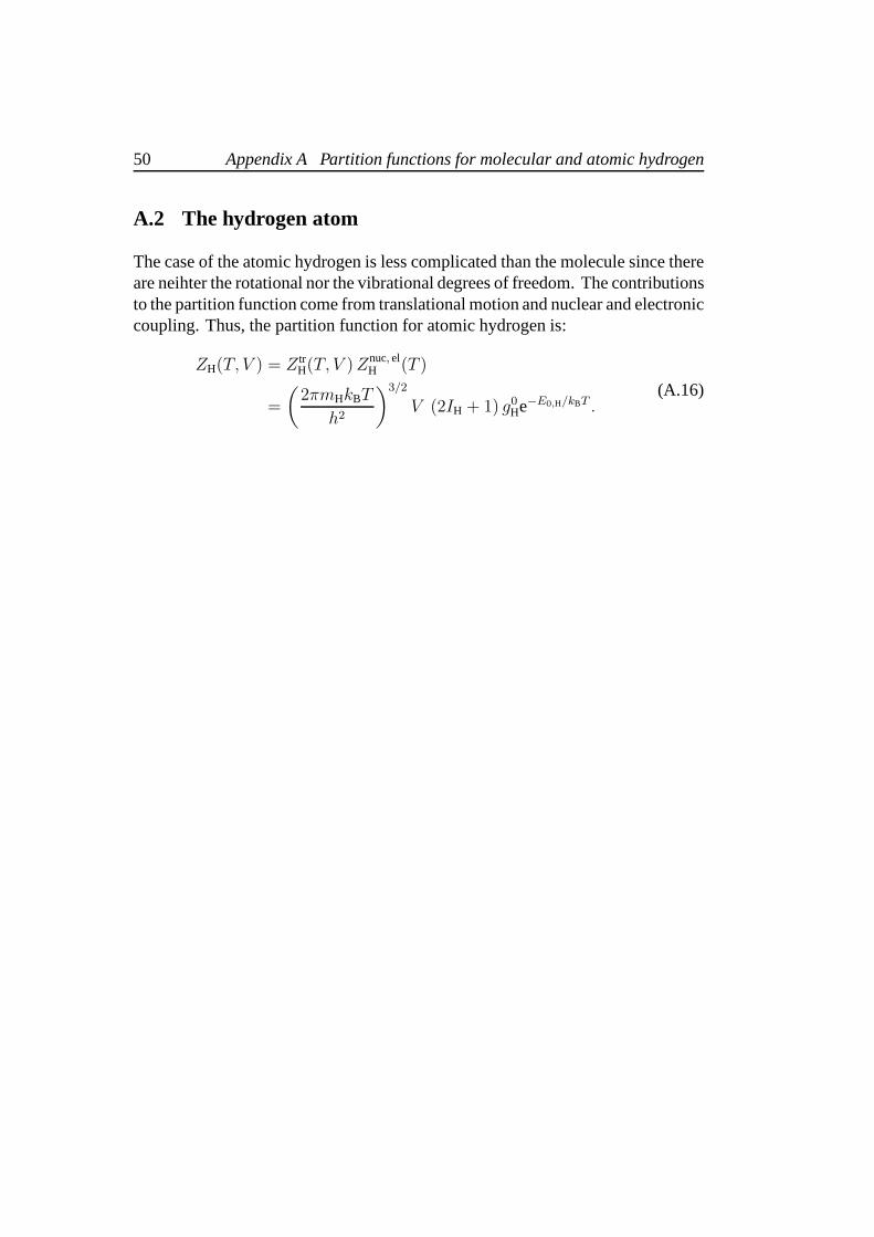
50 Appendix A Partition functions for molecular and atomic hydrogen
A.2 The hydrogen atom
The case of the atomic hydrogen is less complicated than the molecule since thereare neihter the rotational nor the vibrational degrees of freedom. The contributionsto the partition function come from translational motion and nuclear and electroniccoupling. Thus, the partition function for atomic hydrogenis:
ZH(T, V ) = Z trH(T, V )Znuc, el
H (T )
=
(
2πmHkBT
h2
)3/2
V (2IH + 1) g0He−E0,H/kBT .
(A.16)
References
[1] L. Quartapelle and A. Muzzio.Hydrogen ideal gas thermodynamics withdissociation. Unpublished, 2010.
[2] L. Quartapelle and F. Auteri.Fluidodinamica. Unpublished.
[3] P.M. Morse. Diatomic molecules according to the wave mechanics. II. Vi-brational levels. Physical Review, 34:57–64, 1929.
[4] L. Quartapelle, L. Castelletti, A. Guardone, and G. Quaranta. Solution ofthe Riemann problem of classical gasdynamics.Journal of ComputationalPhysics, 190:118–140, 2003.
[5] C.G. Miller III and S.E. Wilder. Table and charts of equilibrium normal-shock properties for pure hydrogen with velocities to70 km/s, 1976. LangleyResearch Center, NASA.
[6] H.B. Callen. Thermodynamics and an Introduction to Thermostatistics.John Wiley & Sons, Second edition, 1985.
[7] L. Galgani and A. Scotti. On subadditivity and convexityproperties of ther-modynamic functions. Pure and Applied Chemistry, 22:229–235, 1970.
[8] Y.B. Zel’dovich and Y.P. Raizer. Physics of Shock Waves and High-Temperature Hydrodynamic Phenomena. Dover Publication, Dover edition,2002.
[9] R.J. Le Roy, S.G. Chapman, and F.R.W. McCourt. Accurate thermodynamicproperties of the six isotopomers of diatomic hydrogen.Journal of PhysicalChemistry, 94:923–929, 1990.
[10] R. Kubo. Statistical Mechanics. North Holland, 1965.
[11] J.W. Leachman, R.T. Jacobsen, S.G. Penoncello, and E.W. Lemmon. Funda-mental equations of state for parahydrogen, normal hydrogen, and orthohy-drogen. Journal of Physical and Chemical Reference Data, 38(9):721–748,2009.
[12] P.A. Thompson. A fundamental derivative in gasdynamics. The Physics ofFluids, 14(9):1843–1849, 1971.
[13] W.G. Vincenti and C.H. Kruger. Introduction to Physical Gas Dynamics.Krieger Publishing Company, 1975.
51
52 References
[14] J.D. Anderson Jr. Hypersonic and High Temperature Gas Dynamics. AIAAEducation, Second edition, 2006.
[15] J.W. Bates and D.C. Montgomery. Some numerical studiesof exotic shockwave behaviour. Physics of Fluids, 11(2):462–475, 1999.
[16] P.L. Roe. Approximate Riemann solvers, parameter vectors, and differenceschemes. Journal of Computational Physics, 43(2):357–372, 1981.
[17] P. Atkins and R. Friedman. Molecular Quantum Mechanics. Oxford Uni-versity Press, 2005.
[18] C. Berkdemir and J. Han. Any l-state solutions of the Morse potentialthrough the Pekeris approximation and Nikiforov–Uvarov method. Chem-ical Physics Letters, 409:203–207, 2005.
[19] S.M. Ikhdair. Rotation and vibration of diatomic molecule in the spatially-dependent mass Schrödinger equation with generalized q-deformed Morsepotential. Chemical Physics, 361:9–17, 2009.
[20] I. Nasser, M.S. Abdelmonem, H. Bahlouli, and A.D. Alhaidari. The rotatingMorse potential model for diatomic molecules in the tridiagonal J-matrixrepresentation. Journal of Physics B, 40:4245–4257, 2007.
[21] E. Castro, J.L. Paz, and P. Martin. Analytical approximations to the eigen-values of the Morse potential with centrifugal terms.Journal of MolecularStructure, 769:15–18, 2006.
[22] D.C. Harris and M.D. Bertolucci. Symmetry and Spectroscopy. DoverPubblications, 1989.
[23] G.V. Yukhnevich. On application of the Morse potentialfor Evaluating anhar-monic vibrations of polyatomic molecules withXHn-complexes. DokladyPhysics, 372(3):322–325, 2000.
[24] D.M. Bishop and S. Shih. An effective Schrödinger equation for the rovi-bronic energies ofH2 andD2. Journal of Chemical Physics, 64(1):162–169,1976.
[25] D.A. Morales. Energy eigenstates of the rotating Morseoscillator using theshifted1/N expansion. Chemical Physics Letters, 161(3):253–258, 1989.
[26] H.W. Woolley, R.B. Scott, and F.G. Brickwedde. Compilation of the ThermalProperties of Hydrogen in its Various Isotopic and Ortho-Para Modifications.Journal of Research of the National Bureau of Standards, 41:379–475, 1948.
References 53
[27] R.J. LeVeque. Numerical Methods for Conservation Laws. Birkhauser,Second edition, 2008.
[28] L.D. Landau and E.M. Lifshitz. Fluid Mechanics. Butterworth-Heinemann,Second edition, 1987.
[29] F.J. Gordillo-Vázquez and J.A. Kunc. Statistical-mechanical calculationsof thermal properties of diatomic gases. Journal of Applied Physics,84(9):4693–4703, 1998.
[30] J.P. Killingbeck, A. Grosjean, and G. Jolicard. The Morse potential withangular momentum. Journal of Chemical Physics, 116(1):447–448, 2002.