spreadsheet modeling of optimum maintenance …€¦ · study case. the optimum preventive...

Spreadsheet modeling of optimum maintenancestrategy for marine machinery in wear-outphase subject to distance between ports as oneof the maintenance constraints

K. B. Artanal, K. Ishida2lGraduate student, Kobe University of Mercantile Marine, Japan2Department of Electro Mechanical and Energy Engineering,Kobe Universi@ of Mercantile Marine, Japan

Abstract

This paper addresses a method in determining the optimum maintenanceschedule for components in wear-out phase, The optimum interval betweenmaintenance for a certain component is optimized based upon the minimum totalcost (the objective fimction) resulted by decision on either that component needsto be replaced by a new one or only requires a preventive maintenance action.That decision is determined by verifying the reliability and availability index ofthat component at each maintenance time. Premium Solver Platform (PSP) isutilized to model the optimization problem. The model takes a finite and equalinterval between maintenance, and the increase of operation cost andmaintenance cost due to deterioration of components is taken into account. Ananalysis on a liquid ring primer (LRP) of a bilge system of a ship is taken as thestudy case. The optimum preventive maintenance schedule is directed to bringinto agreement with the decision that has been taken on the ship’s general surveyschedule,

1 Introduction

The emergence on practical method to set an optimum marine machinerymaintenance program is becoming crucial with the trend of many small shippingcompanies buying second hand ships, doing minimum modification to comply

© 2002 WIT Press, Ashurst Lodge, Southampton, SO40 7AA, UK. All rights reserved.Web: www.witpress.com Email [email protected] from: Maritime Engineering and Ports III, CA Brebbia & G Sciutto (Editors).ISBN 1-85312-923-2

226 MaritimeEngineering& Ports III

with the modem regulation, and treating the machinery as if they are new ones.As a result, an impressive increase on the operating cost as well as themaintenance cost become apparent.

The optimization of maintenance decision making can be defined as anattempt to resolve the conflicts of a decision situation in such a way that thevariables under the control of the decision-maker take their best possible value[1]. One of the controllable variables in the case of machinery maintenance is theinterval between maintenance, The optimum value is achieved when the workingarea of the optimization problem, which is set by constraints, is satisfied. Chiang[2] and Zhang [3] employ MARKOV model to set the reliability and availabilityas the constraints on determination of the optimal maintenance policy and failurefrequency, This approach is only applicable to system or components havingconstant hazard rate, wherein the probability of making transition between twostates remains constant. In the case of wear out components, the reliability of thecomponent hardly achieves the same performance as the condition of theprevious maintenance, It is not a wise decision, therefore, to disregard thedecreasing performance of the component in the optimization model.

In the case where there is uncertainty in the value of the distributionparameter, a Bayesian approach could be used to formally express the uncertainparameters as proposed by Sheu [4] and Apeland [5], If the random variable ofanalyzed data is on hand, the Maximum Likelihood Estimation (MLE) can beused to obtain the distribution parameter, as used in this paper on the liquid ringprimer of a bilge system of a ship,

This paper is aimed to provide a practical method in constructing an optimummarine machinery maintenance schedule. Spreadsheet modeling is one of thealternatives, and will be adopted in this paper. This method needs no painfhl andexhaustive effort to produce programming codes, especially when the problemand optimization model have been well defined [6]. In this paper, non linearprogramming (NLP) can express the problem, and Generalized ReducedGradient (GRG) method can be effectively used to work with the NLPsproblems, as used by the Premium Solver Platform (PSP).

2 Problem description

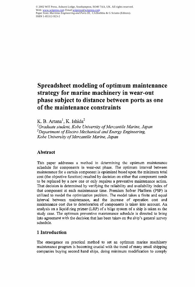
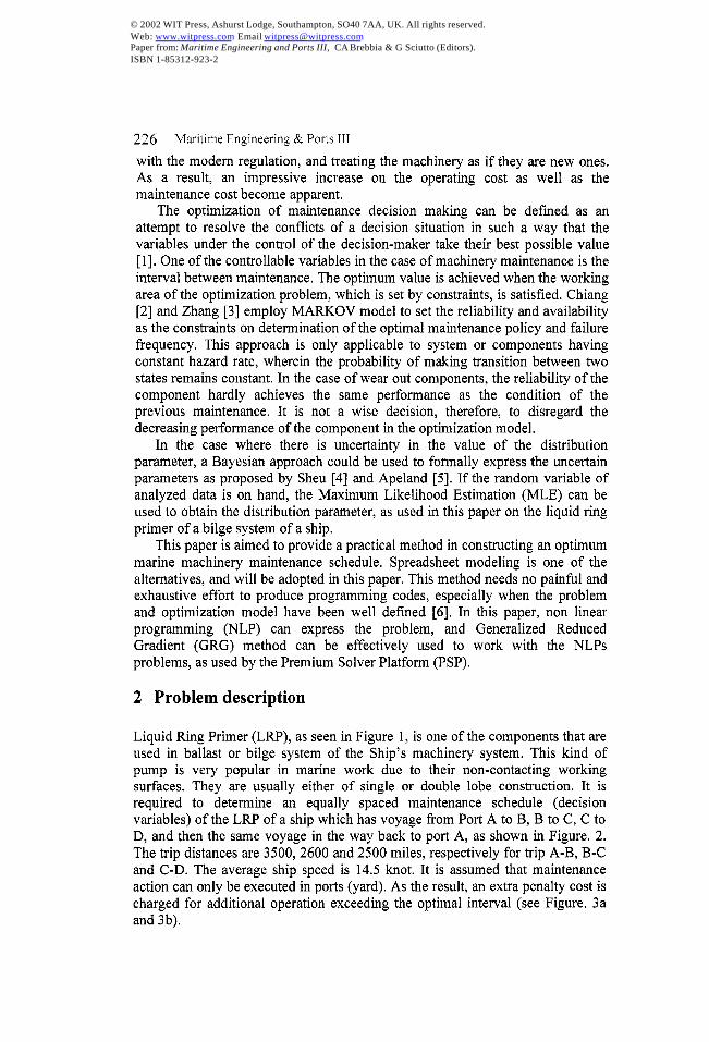
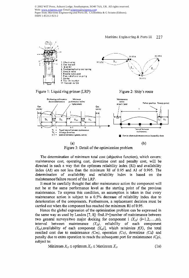
Liquid Ring Primer (LRP), as seen in Figure 1, k one of the components that areused in ballast or bilge system of the Ship’s machinery system. This kind ofpump is very popular in marine work due to their non-contacting workingsurfaces. They are usually either of single or double lobe construction. It isrequired to determine an equally spaced maintenance schedule (decisionvariables) of the LRP of a ship which has voyage tlom Port A to B, B to C, C toD, and then the same voyage in the way back to port A, as shown in Figure, 2.The trip distances are 3500,2600 and 2500 miles, respectively for trip A-B, B-Cand C-D. The average ship speed is 14.5 knot. It is assumed that maintenanceaction can only be executed in ports (yard). As the result, an extra penalty cost ischarged for additional operation exceeding the optimal interval (see Figure. 3aand 3b).


Maritime Engineering & Ports III 22’7

,.y= 4

1/” ,31.. L>

1 Check vabe2 Coolilgooll3, Impelkr4. Mechanka lpu~psealsprng5. Needkvake6 Need kva be seat7 Pum P shaftand coupling8 Spri7g9 Vacuum breaker10 Vacuum sw tih

Figure 1: Liquid ring primer (LRP) Figure 2: Ship’s route

Decreasing perf.onnance Mininwndue to deterioration perfonnanc. before

‘n” / /mp’aceme”’ ::.,Urwy

,------- +,,,,:,...,,,, ...,... ,. ,,, ,,./ Trl ~ Tr2 e Trn.l g Trn

‘\ <1 , “ .

>,

0 ------- ~ ➤n-l n T

Tr = Equal interval b.tw.e” tnai”te”a”ceTd = Average downtimeo.T = l“terwi betwe” 2 general wrvey

Maintenanceaction

at POl’t/ yardFailure position Penalty period

k,,

Int.rval between3

tnainte”a”ce

❑ Port i“ where tnaintena”ce action is powibly done

(a) (b)Figure 3: Detail of the optimization problem

The determination of minimum total cost (objective fimction), which covers:maintenance cost, operating cost, downtime cost and penalty cost, will bedirected in such a way that the optimum reliability index (RI) and availabilityindex (AI) are not less than the minimum RI of 0.95 and AI of 0.995, Thedetermination of availability and reliability index is based on themaintenance/failure record of the LRP.

It must be carefidly thought that after maintenance action the component willnot be at the same performance level as the starting point of the previousmaintenance. To express this condition, an assumption is taken in that everymaintenance action is subject to a 0.5°/0 decrease of reliability index due todeterioration of the components, Furthermore, a replacement decision must becarried out when the component has reached the minimum RI of 0,95.

Hence the global expression of the optimization problem can be expressed inthe same way as used by Lasdon [7, 8]: fmd X=[number of maintenance betweentwo general surveys/two major docking for component i (Xl) (i=l ,2,.,. .,m),interval between maintenance (X,J, reliability of each component(XJ,availability of each component (’J], which minimize ~(X), the totalresulted cost due to maintenance (Cm), operation (Co), downtime (Cd) andpenalty due to extra operation to reach the subsequent port for maintenance (Cp),subject to:

Minimum Xlis optimum Xli s Maximum Xli (la)


228 Maritime Engineering & Ports III

Minimum Xjis optimum Xzi< Maximum X2i (lb)Minimum Xji < optimum Xji < Maximum X3i (lC)Minimum X4i< optimum X4iS Maximum X4i (id)X,i = Integer (le)

The total cost between two general surveys will be a fimction of the intervalbetween maintenance (C(Tr))and can be written as

C(Tr)= Cm+Co+Cd+Cp (2)

where Cm, Co, Cd and Cp are the total maintenance cost, total operating cost,total cost as result of downtime and total penalty cost respectively, for allcomponents under evaluation as a function of Tr, between two general surveys.

Tr

Cm=~ni.f

Cumi (t)dt (3)isl o

Tr

co= : (ni + 1).fcUOi (t)dt (4)/=1 o

ni = number of maintenance of iti component between two general surveyCumi(zj = maintenance cost of ithcomponent per unit time (hour) at time tafter

the last maintenanceni+l = number of interval between two general surveysCuoi(fl = operating cost of i’hcomponent per unit time (hour) at time tafter the

last maintenance111

Cd= ~ ni .Cudi (5)icl

Cudi = cost as a result of downtime of ithcomponent between two generalsurveys

?}1

Cp = ~Tpi.Cupi (6)i=l

Tpi = accumulation of extra operating time of ithcomponent to reach thesubsequent port for maintenance within two general surveys

Cllpi = unit penalty cost of iti componentEquation (2) therefore can be written as

Tr Tr

C(T~) = ~ ni . fcumi (t)dt +(ni +1).~uoi (t)dt +ni.Cudi +tTpi .Cupi (7)j=l o 0

Due to component’s deterioration, the maintenance cost and operating costper hour are assumed increase exponentially with use of the form ofl

Cumi (t)= Ai - Bi .eXp(-kj .t) (8)

CUOi (t)= Ej - Fi . exp(-li .t) (9)

where (A-B), (E-F) may be interpreted as the maintenance cost and operatingcost per unit time (hour) if no deterioration occurs. k, 1 are growthfactor/constant which specifies the shape of the curve. Substituting equation (8)


Maritime Engineering & Ports III 229

and (9) to (7) gives the complete declaration of the total cost (objective f unction)as below:

111

C(Tr) = ~ niAiTri +m(e~p(-kiTri )-1)+ (n, +l)E,Tri +icl ki

(ni +l)Fi~, (exp(-l,Tri )-l)+ ni.(kz’i + Tpi.Czqi

where the ;utputidecision variable ni can be expressed by (see Figure. 3a):

T – Trini =

Tri +Tdi

(10)

(11)

If it is assumed that the component’s downtime (Tc# is constant, then theproblem becomes minimization of total cost (C(Tr)) by applying the optimumequally interval maintenance program (Tr).

3 Model construction

The basic format of the offered optimization process can be seen in Figure. 4,Input consists of all parameters, which will be used in the entirely of theoptimization process, For a very complex problem, those parameters can beclassified into several directories so as to make the fault identification easier.Moreover, the use of directories will also make the optimization process easier,since it will design the optimization process and the relationship between eachdirectory become clearer, In this particular problem, input comprises distancebetween port, average ship speed, unit downtime cost, unit penalty cost,reliability reduction factor, component’s failure rate, etc.

All basic calculations for the optimization process (eqn (3-9)) are located inthe “equation folder”, The results of each equation were continuously updatedsince the optimization process in the “constraints” and “output” will alwaysaffect the variables employed on the equation, The equation coversdetermination of operating cost, maintenance cost, number of repair beforereplacement, replacement schedule, position of maintenance, position of end trip,penalty time, etc.

Constraints, which are the considerations to be fulfilled (eqn (lb- 1e)), becomethe director of this optimization process. A minimum or maximum value is set togive the working area of the optimization process. The optimum values arelocated in the center of the form and it will change, as the constraints arechanged. Determination of the minimum or maximum value absolutely dependson the characteristic of the constraints.

Output (equation (1a)) has characteristics, which are nearly the same as theconstraints except that the output are set from decision variables (optimizationresult), which are different with the equation that adopted in the constraints. Themaximum and minimum values are also set to direct the optimization process.



Figure 4: Basic format of the optimization process

All optimization methods have the same pattern in which they formed to fmdeither a maximum or minimum solution of the objective Iimction. Equation (10)shows the expression of the total cost that is the objective fimction of thisparticular problem.

There are several strategies in transferring the model into spreadsheet form.Ragsdale [9] and Monahan [10] can be referred for detail information on thismatter.

4 Data analysis

The maximum likelihood estimate (MLE) method is widely used to obtainparameters of certain distribution if a set of random variable of the analyzed datais available, This paper only considers four distributions: 2-parameterexponential distribution, normal distribution, 2-parameter Weibull distributionand 3-parameter Weibull distribution, The normal distribution is chosen basedupon central limit theorem assumption. The exponential distribution is selecteddue to its failure characteristic represent the usefbl life period in a bath-up curve,While the Weibull distribution is selected due to the flexibility of thedetermination of the parameter that can well de~cribed the failure pattern of thedata that might be laid either on useful life period or wear out period, These fouralternatives are examined to ensure that the LRP’s components being analyzedoperate at wear-out phase, and relevant reliability fimction can be appliedaccordingly.

The input of failure modeling of the LRP is time to failure (TTF), andrecorded based upon its maintenance record. The parameters for eachdistribution are determined by using MLE method. PC-based software was usedto speed up the calculation for obtaining the parameters. The distributionsresulted from a set of LRP time to failure are then compared to choose the fittestone based upon the likelihood value of the MLE. Table 1 shows the results ofMLE analysis and the value of parameters of each distribution that represents


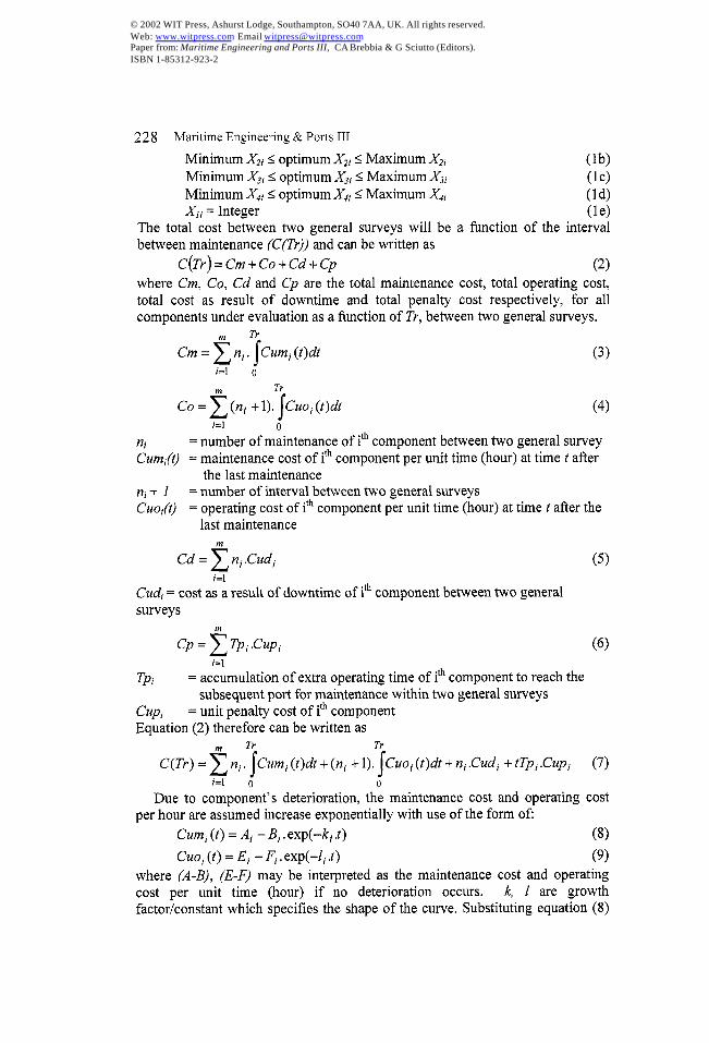
Maritime Engineering & Ports III 231each set TTF data of the LRP and Figure, 6 shows the Reliability and pdf curveof the 5(five) fust components of the liquid ring primer (LRP).

Table 1. MLE evaluation results and Weibull parameter

Components Likelihood value for each Weibull parameter valuesdistribution under evaluation

normal Exp, Weibull Weibull Beta Eta (hrs) Gamma1. Check valve -921,24 -867,5 -866,99 -866.95 4.1661 5747.46 -554.4462. Cooling coil -894,19 -861,7 -861,04 -860.45 2,9047 3974,25 -529,6753. Impeller -819,43 -772,3 -771.96 -771,99 3.939 2162.15 04, Mech, pump seal spr. -848,46 -847.5 -835.93 -836.07 1,6172 2,039,86 05. Needle valve -952.92 -937,1 -932.53 -932,65 2.0326 6236.13 06, Needle valve aeat -892,26 -880,2 -875,83 -875.71 2.092 3605,09 -283.277. Pump ahafl & coupl, -1001,93 -1021,4 -1000.2 -1000,25 1,2511 9031,01 08. Spring -976,23 -963,6 -957.61 -957,63 1,9885 7935.05 09. Vacuum breaker -1029.46 -1041.9 -1023.7 -1024,64 1,4478 12482,50 010, Vacuum switch -1024,49 -983.71 -983,89 -981.98 3,0503 13799,61 -1156.38

As shown in Table 1, the components are clearly in the wear-out periods,since their likelihood values lean toward either 2-parameter Weibull distributionor 3-parameter Weibull distribution (bold type values mean prefemeddistribution) and their shape parameter are greater than 1 (~>1) [11, 12]. Figure.5 shows that for components having value (3>1, then the pdf is zero at t=yincreases as t toward the mean life and decrease thereafter. It is also shown thatthe Weibull reliability tlmction starts at the value of 1 at t=y, and decreasesthereafter for t>y, As ttends toward infinity, then the reliability function headedfor O.For wear-out cases the R(O decreases as tincreases, and for the same valueof (3, component having greater q decreases less sharply than the one havingsmaller value of ~.

The Weibull distribution, in which all of the LRP’s components fit with, isone of the most widely used distributions in reliability engineering. It is becausethe distribution is able to model a great variety of data by adjusting the value ofshape parameter ~. The pdf of three-parameter of Weibull distribution is givenby

0001

D0000

D0000

00001

: 0000s

: 00005

g D00C4m-/ 00003

‘ 0000100001

1,0

0,9

0s

07

03

02

01

(12)

.S000 14600 3$700 55600 76400 97000 I 2E.4 1 4E+4 ao m iwc w 35m.oO

ml,

[1] H 05% @7S4 207! ?SS4 4461 Chwk ‘ialk.)[1] M KC4 q.39m 63.$0, 7-S2$ 6751 0001”, Od[3] #-3 %R2 q.11S9 S6S3 F-99 63% Omdhrl[4] !-1 SS72 w2Cd4 M46 c-992W. :;;:;;SyO[s] $-19442 @267 S648 F-996%

Figure 5: Reliability curve andpdf curve of five (5)

5s0 m 764UQ 97W m 1.1E+a 1.3SE+4

TM

first components of LRP



where

!3= shape parameter, P >0q = scale parameter, T >0y = location parameter, y < fust time to failureThe reliability i?mction of the Weibull distribution can be written as

-[-1(-y D

R(t) = e vand its failure rate can be written as

If YD= O,then the two-parameter of Weibull distribution is obtained.The mean time to failure (MTTF) of Weibull pdf is given by

(13)

(14)

(15)

where r[(l/~)+1 ] is the gamma function evaluated at the value of [(1/~)+1 ],The availability of the component then can be expressed as

Availability =tiTTF

MTTF i- MTTR(16)

Aside from the failure (TTF) data. cost data also need further verification.Based on the data collection process, ‘only the maintenance cost and operationcost of the LRP are available. Due to the fact that it is required to fmd the effectof the each component’s deterioration to the total cost, then we adopt weightingmethod to distribute the total cost into its component’s cost constituents [13, 14],

5 Model analysis

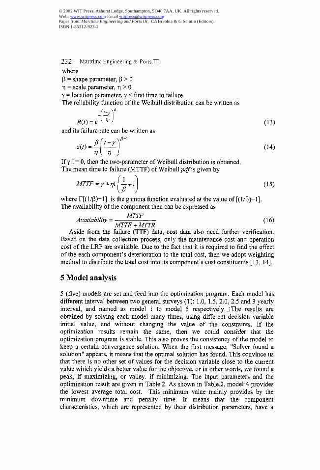
5 (five) models are set and feed into the optimization program. Each model hasdifferent interval between two general surveys (T): 1.0, 1.5, 2.0,2,5 and 3 yearlyinterval, and named as model 1 to model 5 respectively. LThe results areobtained by solving each model many times, using different decision variableinitial value, and without changing the value of the constraints. If theoptimization results remain the same, then’ we could consider that theoptimization program is stable. This also proves the consistency of the model tokeep a certain convergence solution. When the first message, “Solver found asolution” appears, it means that the optimal solution has found. This convince usthat there is no other set of values for the decision variable close to the currentvalue which yields a better vaIue for the objective, or in other words, we found apeak, if maximizing, or valley, if minimizing, The input parameters and theoptimization result are given in Table,2. As shown in Table.2, model 4 providesthe lowest average total cost. This minimum value mainly provides by theminimum downtime and penalty time. It means that the componentcharacteristics, which are represented by their distribution parameters, have a



better agreement with the equally-interval between maintenance for a 2,5 yearlygeneral survey.

Table 2. Cost recapitulation for each model

INPUT reliability decrease factor 0,995minimum req. availability index 0,95 port c-port d distance miles 2500minimum req. reliability index 0.995 average ship speed knot 14,5port a-port b distance miles 3500 unit cost of downtime $ 150port b-port c distance miles 2600 unit ext. cost for ext. utilization $llms 0,1

interval total total total total total Ave.between 2 operating maint. downtime Penalty cost total

surveys cost cost cost cost cost

(years) ($) ($) ($) ($)model 1

($)1,0

($lmth)1559,73 160.50 450.00 379,43 2,549, 212,47

model 2 1,5 2506,10 215,41 750.00 533.69 4,005. 222,51model 3 2,0 3122,65 453.51 1500,00 780,72 5,856, 244.04model 4 2,5 3938,08 577,08 900.00 866.53 6,281,model 5 3.0

209,394504,48 856.54 2850.00 1503,17 9,714, 269,84

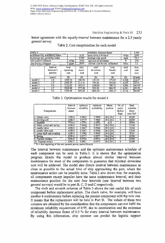
Table 3. Optimization results for model 4

interval optimum optimum Maint, No. of Repl.between reliability availability position maint, schedule

Components maint, Before (fromRepl. next Ts)*

1. Check valve 4380,0 0,9801 0,9968 B-C-D-C 6 262802 Cnn!in ~ cOil 4380.0 0.9779 09966 R.C..D.C (i 26280

7wm n n 976A,.Ay “.- .Y . . ..a 1 ,. ..,- .

1,,. Al!/nn I oe...-10, VU-”-L... .. ... .. T. ..,.* Ts = the beginning of tbe next general SU]

+

. -r....= ..-.,.. . .0 VacmnZIbresker I 4380,0 I 0,9725

l.., m,m ,,,,:f,.h d~m n n OQm-1-rvey

. . . . . -----. . . 0.9992 – ‘ii - i 36500fl,9642 0,9975 B-C-D-C 3 13140..9667 0.9964 B-C-D-C 3 131400,9667 0,9968 B-C-D-C 3 131400,9582 0.9959 B-C-D-C 2 8760n 9771 0,9975 B-C-D-C 6 26280

0,9973 B-C-D-C 5 21900., .-. . 0,9973 B-C-D-C 6 26280

period (honrs)

The interval between maintenance and the optimum maintenance schedule ofeach component can be seen in Table.3. It is shown that the optimizationprogram directs the model to produce almost similar interval betweenmaintenance for most of the components to guarantee that minimal downtimecost will be achieved, The model also directs interval between maintenance asclose as possible to the actual time of ship approaching the port, where themaintenance action can be possibly done. Table.3 also shows that, for example,all components except impeller have the same maintenance interval, and theirmaintenance position for the next four intervals (one interval between twogeneral surveys) would be in port B, C, D and C respectively.

The sixth and seventh columns of Table 3 shows the rest useful life of eachcomponent before replacement action. The check valve, for example, will haveanother 6 maintenance before replacing the present component with the new one.It means that the replacement will be held in Port D, The values of these twocolumns are obtained by the consideration that the components can not fulfil theminimum reliability requirement of 0.95, due to deterioration and the existenceof reliability decrease factor of 0,5 0/0for every interval between maintenance.By using this information, ship operator can predict the logistic support



accordingly, The other general feature of the optimization result is that theincrease in interval between maintenance result in the increase of the operatingcost, and at the same time reduces the maintenance cost. The increase in intervalbe~een maintenance will then be limited by the requirement to perform aminimum value of reliability index for each component,

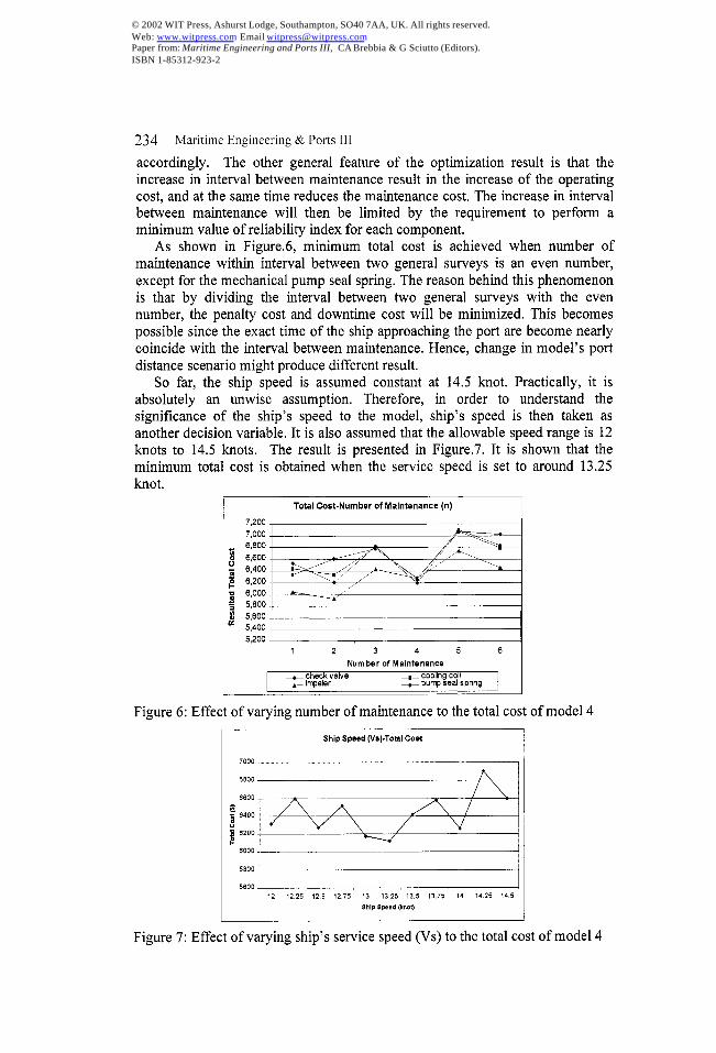
As shown in Figure,6, minimum total cost is achieved when number ofmaintenance within interval between two general surveys is an even number,except for the mechanical pump seal spring. The reason behind this phenomenonis that by dividing the interval between two general surveys with the evennumber, the penalty cost and downtime cost will be minimized. This becomespossible since the exact time of the ship approaching the port are become nearlycoincide with the interval between maintenance. Hence, change in model’s portdistance scenario might produce different result.

So far, the ship speed is assumed constant at 14.5 knot. Practically, it isabsolutely an unwise assumption. Therefore, in order to understand thesignificance of the ship’s speed to the model, ship’s speed is then taken asanother decision variable. It is also assumed that the allowable speed range is 12knots to 14.5 knots. The result is presented in Figure.7. It is shown that theminimum total cost is obtained when the service speed is set to around 13.25knot.

I TotalCost-Number of Maintenance (n)

6,000/

A

5,800‘A

~

5,6005,400 ~5200 ~

1 2 3 4 5 6

Numbar of Maintenance

- ?hackvalve - coohgcOIl- rrpelar - PUT saal spring ~

Figure 6: Effect of varying number of maintenance to the total cost of model 4

6000. I

6800.

5600,

12 12,25 12,5 12,75 13 1325 13,5 13,75 14 ?425 ?45

8hlp SPeed (knofl

Figure 7: Effect of varying ship’s service speed (Vs) to the total cost of model 4



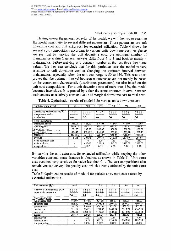
Having known the general behavior of the model, we will then try to examinethe model sensitivity to several different parameters. Those parameters are unitdowntime cost and unit extra cost for extended utilization. Table 4 shows theseveral cost compositions according to various units downtime cost, At glancewe see that by varying the unit downtime cost, the optimum number ofmaintenance within 2 general surveys shifts from 4 to 3 and back to mostly 4maintenance, before arriving at a constant number at the last three downtimevalues. We then can conclude that for this particular case the model is verysensitive to unit downtime cost in changing the optimum interval betweenmaintenance, especially when the unit cost range is 50 to 150. This result alsoproves that the optimum interval between maintenance can not merely be basedon the component characteristic (distribution parameters) but also based on theunit cost compositions. For a unit downtime cost of more than 150, the modelbecomes insensitive, It is proved by either the same optimum interval betweenmaintenance or relatively constant value of marginal downtime cost to total cost,

Table 4. Optimization results of model 4 for various units downtime cost

Unit downtime cost ($) I 50 I 100 I 150 I 200 I 250 I 300

Number of maintenance of 10 4-4-4-4- 3-3-3-3- 4-4-2-4- 3-3-3-3- 3-3-3-3- 3-3-3-3-cornponentsunder 4-4-4-4- 3-3-3-3- 4-4-4-4- 3-3-3-3- 3-3-3-3- 3-3-3-3-evaluation 4-4 3-3 4-4 3-4 3-4 3-4

maintenance cost 586,01 464,07 577,08 478,07 478,07 478.07operating cost 3909.10 4142,27 3938,08 4135,32 4135.32 4135,32downtime cost 200.00 300,00 900,00 1400,00 1750,00 2100,00penalty cost 829.45 1305,29 866,53 1253,20 1253,20 1208.19total cost 5524.56 6211,62 6281,69 7266,59 7616,59 7921.58

-,---n- .- .,.- , -...05 209.39 242,22 253,89 264,05delta downtime cost ~ 50 100 150 200 250,,, ,,, . ,“.. . . 757.13 1742.03 2092.03 2397,02

margmal vame I I U,UI I 0,13 0,09 0,10 0,10aelra roral cost I I 051,U0 I.,. ..-

By varying the unit extra cost for extended utilization while keeping the othervariables constant, some features is obtained as shown in Table 5. Unit extracost becomes very sensitive for value less than 0.1, The cost compositions alsoremain constant except the penalty cost, which directly affected by the unit extracost.Table 5, Optimization results of model 4 for various units extra cost caused byextended utilization

Unit extra cost ($)ihr 0.05 0,1 0.2 0,3 0.4 0,5

Number of maintenance of 10 3-3-3-3- 4-4-2-4- 4-4-2-4- 4-4-4-4- 4-4-4-4- 4-4-4-4-

parts under evaluation 3-3-3-3- 4-4-4-4- 4-4-4-4- 4-4-4-4- 4-4-4-4- 4-4-4-4-3-4 4.4 4-4 4-4 4-4 4-4

Cost constituentsmaintenance cost 478,07 577.08 577,08 586,01 586,01 586,01operating cost 4135.32 3938,08 3938.08 3909.10 3909.10 3909,10downtime cost 1050,00 900,00 900.00 600,00 600.00 600.00penalty cost 581.59 866,53 1761,90 2488,34 3317.78 4147,23total cost 6244,98 6281,69 7177.06 7583.45 8412,90 9242,34average 208.17 209.39 239,24 252.78 280.43 308,08delta dh cost 0,05 0,15 0.25 0,35 0,45delta total cost 36,71 932.08 1338,47 2167.92 2997.36marginal value 0,0014 0,0002 0,0002 0,0002 0,0002



6 Conclusion

In the present article, a spreadsheet model has been developed and used todetermine the optimum maintenance schedule for several liquid ring primercomponents of a ballast system of ships, which has been entering a wear-outphase. The PSP is employed to simulate 5 models having different intervalbetween two general surveys, The optimal policy is defined as the one thatminimize the total cost which comprises maintenance cost, operating cost,downtime cost and penalty cost.

The simulation results show that with the existing condition of thecomponents, as represented by their Weibull distribution parameters, the 2.5yearly interval between two surveys is the scenario that provides minimum totalcost. Sensitivity analysis on the effect of unit downtime cost and unit penaltycost shows that the equally interval maintenance scheme can not be decided byconsidering the components characteristics only, but also must take the operationcondition into account, In this paper, the operating condition comprises shiproute, technical maintenance policy, and unit cost composition that are adoptedwithin the model. Effect of the decrease of components performance andreliability index due to, deterioration has also been considered in the model.Therefore, spare parts and other logistic supports can be prepared accordingly.

Generally speaking, the difficulty of using spreadsheet model to solveoptimization problem does not come into spreadsheet construction viewpoint,but lay on the way to express every optimization problem and condition intomathematical expression that can be executed by the spreadsheet. In thisparticular study case, since the unit downtime cost and unit penalty cost effectthe optimization result sensitively, the attention must be paid on the way todetermine those unit costs that reflect the actual ship’s and machinery operationcondition.

Likewise, it is difficult to accurately express the time dependent function ofoperating and maintenance cost as simplified by equation (8) and (9). As thesetwo cost constituents are the main cost components of this particular problem,then we must focus the attention on the preciseness of each constant, or ifpossible, express those two equations in different way, that resembling the realcondition.

References

[1] Jardine, A,K,S., Maintenance, Replacement and Reliability. Great Britain,Pitman Publishing, 1973.

[2] Chiang, J,H,, Yuan, J., Optimal maintenance policy for a Markovian systemunder periodic inspection, Reliability Engineering and System Safety,2001;71:165-172.

[3] Zhang, T., Hiranuma, K., Sate, Y., Horigome, M., Failure frequency andavailability of 3-out of -4 G warm standby systems with non-identicalcomponents. Proceedings of ISME Tokyo 2000;VOL2:805-8 10.


[4]

[5]

[6]

[7]

[8]

[9]

[10]

[11]

[12]

[13]

[14]


Sheu, S,H., Yeh, R.H., Lin, Y.B., Juang, M.G., A Bayesian approach to anadaptive preventive maintenance model. Reliability Engineering andSystem Safety, 2001; 71:33-44.Apeland, S., Aven, T,, Risk based maintenance optimization: foundationalissues. Reliability Engineering and System Safety, 2000 ;67:285-292.Artana, K.B,, Ishida, K., Determination of ship machinery performance andits maintenance management using Markov process analysis. Proceedingsofklarine Technology 2001 Conference.Lasdon, L.S., Waren, A.D., Jain, A., Ratner, M., Design and testing of ageneralized reduced gradient code for nonlinear programming. ACMTransactions on Mathematical Sofware, 1978; 4:34-49.Lasdon, L.S,, Smith, S,, Solving large sparse nonlinear programs usingGRG, ORSA Journal on Computing, 1992; 4:2-15.Monahan, G.E., Management Decision Making: Spreadsheet Modeling,Analysis, and Applications. Cambridge Univ. Press, Jan 2000.Ragsdale, C,, Spreadsheet Modeling and Decision Analysis. South-WesternCollege Publishing, 2000.Hoyland, A., Rausan, M.. System Reliability Theory. John Willey & SonsInc., 1994,Kececioglu, D., Reliability Engineering Handbook Volume 2. New Jersey:Prentice-Hall Inc. 1991,Yang, J.B., Sen, P,, A General multi-level evaluation process for hybridMADM with uncertainty. IEEE Trans. On System, Man, and Cybernetics,1994; 24:1459-1473,Sen, P,, Yang, J.B., Combining objective and subjective factors in multiplecriteria marine design. Proceedings of .?h International Marine DesignConference, 1994:505-519.


spreadsheet modeling of optimum maintenance …€¦ · study case. the optimum preventive...

Documents