SOLAR AND PHOTOVOLTAIC FORECASTING THROUGH POST-PROCESSING OF THE GLOBAL ENVIRONMENTAL MULTISCALE

NUMERICAL WEATHER PREDICTION MODEL

Sophie Pelland1, George Galanis2,3 and George Kallos2

1CanmetENERGY, Natural Resources Canada, Varennes, Québec, Canada 2 Atmospheric Modeling and Weather Forecasting Group, Department of Physics,

University of Athens, Athens, Greece 3 Naval Academy of Greece, Section of Mathematics, Piraeus, Greece

Corresponding e-mail: spelland@nrcan.gc.ca

Keywords: solar forecasting; photovoltaic forecasting; numerical weather prediction; post-processing; Kalman filter; spatial averaging.

ABSTRACT

Hourly solar and photovoltaic (PV) forecasts for horizons between 0 and 48 hours ahead were developed using Environment Canada’s Global Environmental Multiscale (GEM) model. The motivation for this research was to explore PV forecasting in Ontario, Canada where feed-in tariffs are driving rapid growth in installed PV capacity. The solar and PV forecasts were compared to irradiance data from 10 North American ground stations and to AC power data from 3 Canadian PV systems. A one year period was used to train the forecasts and the following year was used for testing. Two post-processing methods were applied to the solar forecasts: spatial averaging and bias removal using a Kalman filter. On average, these two methods lead to a 43% reduction in RMSE over a persistence forecast (skill score = 0.67) and to a 15% reduction in RMSE over the GEM forecasts without post-processing (skill score = 0.28). Bias removal was primarily useful when considering a « regional » forecast for the average irradiance of the 10 ground stations, since bias was a more significant fraction of RMSE in this case. PV forecast accuracy was influenced mainly by the underlying (horizontal) solar forecast accuracy, with RMSE ranging from 6.4 to 9.2% of rated power for the individual PV systems. About 76% of the PV forecast errors were within +-5% of the rated power for the individual systems, but the largest errors reached up to 44 to 57% of rated power.

1. INTRODUCTION

In order to integrate large amounts of intermittent renewable generation reliably and cost-effectively into electricity grids, system operators need both to understand the variability of these generators and to be able to forecast this variability at different spatial and temporal scales. While the timescales relevant for forecasting vary, most system operators use a day-ahead commitment process to commit generators to meet the next day’s forecasted load. Moving closer to real time, updated conditions and forecasts are used to dispatch generators, secure reserves and lock in imports and exports. Meanwhile, the geographic area of interest for forecasting can vary from a large area over which

electricity supply and demand must be balanced to a much smaller region where grid congestion must be managed.

The motivation for the research presented here was the introduction of feed-in tariffs in the province of Ontario, Canada [1] which lead to a rapid increase in the contracted and installed capacity of photovoltaics and other renewables in Ontario. The Ontario Independent Electricity System Operator (IESO) recently put forward a call for proposals to develop centralized wind forecasting for the province, which has an installed wind capacity of over 1.1 GW and a peak load of about 27 GW. Meanwhile, contracts for over 1 GW of PV systems have been offered under the Feed-In Tariff Program [1] and PV forecasting implementation should begin once installed PV capacity becomes comparable to the (current) installed wind capacity.

While many system operators around the world have implemented wind forecasting, solar forecasting is comparatively recent. One interesting implementation is taking place in Germany: at the end of 2008, two German transmission system operators with (at the time) 2.9 GW of installed PV corresponding to over 200 000 systems across their balancing areas mandated different forecast providers to implement and test PV forecasts for their balancing areas. The University of Oldenburg and Meteocontrol GmbH have reported results from their ongoing forecast evaluations in [2]. As in the case of wind forecasting, research from the University of Oldenburg shows that solar and PV forecast accuracy improves significantly as the size of the geographic area under consideration increases, with a reduction in root mean square error (RMSE) of about 64% for a forecast over an area the size of Germany as compared to a point forecast [3]. This effect was modelled in detail by Focken et al. [4] in the case of wind. They showed that both the size of the geographic area and the number of stations or systems considered contributed to error reduction, with the reduction from an increased number of stations saturating beyond a certain threshold for a given geographic area. For both PV and wind forecasting, the most appropriate approach depends on the forecast horizon: for forecast horizons of about 0 to 6 hours ahead, methods based primarily on observations (from ground stations or satellites) tend to perform best, while for forecast horizons of about 6 hours to a few days ahead global numerical weather prediction models become more accurate [5].

The approach described in this paper focuses on 0-48h ahead forecasts based on post-processing of a global numerical weather prediction model, namely Environment Canada’s Global Environmental Multiscale (GEM) model. The GEM forecasts and the solar and PV data used for comparisons are described in Section 2, along with the quality check procedures that were applied to the data. Section 3 presents the post-processing (spatial averaging and Kalman filter) that was performed to improve the forecast accuracy. Section 4 examines the accuracy of the forecasts and the distribution of forecast errors, as well as the increase in forecast skill through post-processing; this is followed by concluding comments in Section 5.

2. SOLAR FORECASTS AND DATA USED FOR FORECAST EVALUATION

2.1 GEM weather forecasts

Environment Canada’s Canadian Meteorological Centre operates a global numerical weather prediction model known as the Global Environmental Multiscale (GEM) model (see [6]). The model is run in different configurations, including a configuration known as the “high resolution regional run” which generates forecasts for horizons between 0 and 48 hours ahead at a 7.5 minute timestep over a variable spatial resolution grid, with a spatial resolution reaching about 15 km at the grid centre, in Canada. Model runs are initiated up to four times a day, at 0 UTC, 6 UTC, 12 UTC and 18 UTC, and a subset of model outputs are made available online at timesteps of 3 hours or more [7]. For the purpose of this analysis, the Canadian Meteorological Centre de-archived past forecasts from the high resolution regional run at an hourly timestep over the 2 year period between April 1, 2007 and March 31, 2009 for several weather variables, including downward shortwave radiation flux at the surface (DSWRF), temperature at 2m above the surface (TMP) and total cloud cover (TCDC) [7]. The de-archived forecasts cover North America and adjacent waters.

Only forecasts originating at 12 UTC were considered here, since these are the most relevant for day-ahead PV forecasting in Ontario: currently, generators (of 20 MW or more) are asked by the Ontario Independent Electricity System Operator (IESO) to produce forecasts by 11AM for each hour of the following day, which means that 12 UTC (7AM EST in Ontario) forecasts are the most recent forecasts available prior to the 11AM deadline. The day-ahead IESO forecast period corresponds to forecast horizons of 17 to 41 hours ahead in the GEM 12 UTC forecast. Forecasts were provided in Grib1 format, and were extracted for the variables and grid points of interest using the open source program read_grid [8] in Matlab.

2.2 Ground station irradiance data and data quality check procedure

The stations shown on the map in Figure 1 were selected to test the accuracy of the GEM regional solar forecasts. In Canada, the three stations selected measure direct, sky diffuse and global horizontal irradiance (GHI) each second, with one minute averages and standard deviations being recorded. These stations are operated by Environment Canada and by Natural Resources Canada, with stations being maintained on a daily basis. Similarly, the seven U.S. stations selected measure global horizontal, sky diffuse and direct irradiance every three minutes up to January 2009, and every minute after that. The seven U.S. stations comprise the U.S. Surface Radiation Budget (SURFRAD) network [9]. Along with the station at Bratt’s Lake, these are part of the Baseline Surface Radiation Network (BSRN), a worldwide network of research grade radiation measurement stations.

Since solar forecasts were obtained on an hourly basis, the 1-3 minute ground station data was averaged hourly as well, and quality check procedures were applied to the hourly averages. The quality check procedures that were applied are a subset of those described in tables 1 and 2 of [10]. Global horizontal irradiance values were excluded from the analysis when these were outside a physically plausible range. Similarly, data was

dismissed if diffuse irradiance measurements were greater than global horizontal irradiance measurements by more than 5 or 10 % (depending on the zenith angle).

• Bratt’s Lake, SA

• Varennes, QC

• Egbert, ON

• Desert Rock, NV

• Goodwin Creek, MS

• Bondville, IL• Penn State, PA

• Fort Peck, MT

• Sioux Falls, SD

• Boulder, CO

• Bratt’s Lake, SA

• Varennes, QC

• Egbert, ON

• Desert Rock, NV

• Goodwin Creek, MS

• Bondville, IL• Penn State, PA

• Fort Peck, MT

• Sioux Falls, SD

• Boulder, CO

Figure 1: Map showing the location of the 3 Canadian and 7 US meteorological

ground stations used in this analysis.

2.3 Photovoltaic system data and data quality check procedure

Table 1 shows key properties of the three PV systems that were used to test the PV forecasts. For simplicity, forecasts were generated for the hourly average AC power output of a single inverter, so in the case of the Exhibition Place and Varennes PV systems the data considered is from a single sub-array that is part of a larger PV system. The extent and quality of the monitoring is different for each of these systems, but all of them include sub-hourly monitoring of AC (and DC) power, which was used to generate hourly averaged values against which to verify the PV forecasts.

Various quality check procedures were applied to the data, including flags corresponding to specific situations of interest:

When the AC power dropped to zero (or less) for an extended period while irradiance was non-zero, this was flagged as an outage.

Using Environment Canada’s Climate Data Online [11], days surrounding significant snowfall events at the ground station nearest to each PV system were singled out for further study. Visual inspection of the data was used to assign a

tentative snow cover flag, with snow cover being flagged when a noticeable drop in the daily performance ratio coincided with snowfall.

Days flagged for snow cover were included in the testing period, but the snow flags were used to determine the impact of these events on forecast accuracy. Meanwhile, outages were excluded from the PV forecast evaluation, to reflect the expectation that outages for well-monitored Megawatt scale systems or over ensembles of smaller, independent systems should be quite rare, and taken into account in the forecasting process when they do occur.

Table 1: Key properties of the three Canadian PV systems used to test PV forecasts.

Name of system or sub-array

Location Rated power (DC STC) (kW)

Module type Mounting Orientation

Varennes Varennes, Québec

6.72 Monocrystalline

silicon Rack-mounted

on rooftop South-facing,

45° tilt

Queen’s Kingston, Ontario

19.8 Polycrystalline

silicon Rack-mounted

on façade 5° West of

South, 70° tilt

Exhibition Place

Toronto, Ontario

45.6 Polycrystalline

silicon Rack-mounted

on rooftop 20° East of

South, 20° tilt

3. SOLAR AND PV FORECAST DEVELOPMENT AND TESTING

3.1 Forecast accuracy measures

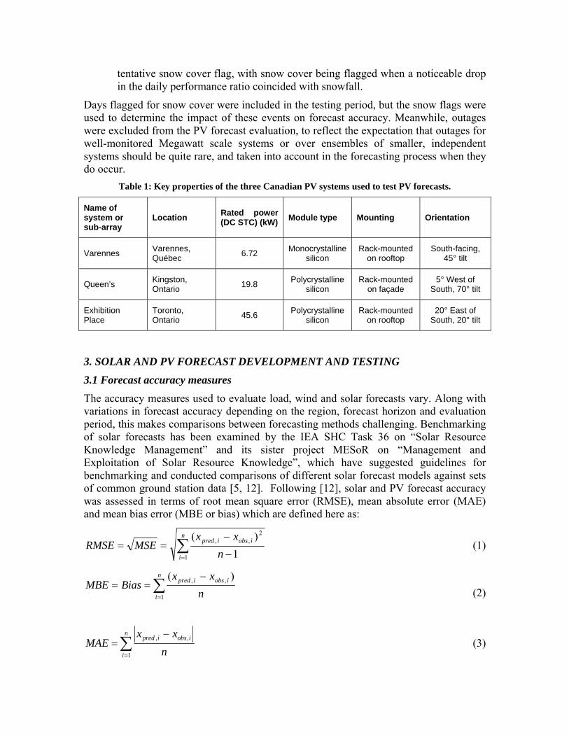
The accuracy measures used to evaluate load, wind and solar forecasts vary. Along with variations in forecast accuracy depending on the region, forecast horizon and evaluation period, this makes comparisons between forecasting methods challenging. Benchmarking of solar forecasts has been examined by the IEA SHC Task 36 on “Solar Resource Knowledge Management” and its sister project MESoR on “Management and Exploitation of Solar Resource Knowledge”, which have suggested guidelines for benchmarking and conducted comparisons of different solar forecast models against sets of common ground station data [5, 12]. Following [12], solar and PV forecast accuracy was assessed in terms of root mean square error (RMSE), mean absolute error (MAE) and mean bias error (MBE or bias) which are defined here as:

n

i

iobsipred

n

xxMSERMSE

1

2,,

1

)( (1)

n

i

iobsipred

n

xxBiasMBE

1

,, )(

(2)

n

i

iobsipred

n

xxMAE

1

,, (3)

where xpred,i and xobs,i represent the ith valid forecast and observation pair, respectively, and where the sums are carried out over all n such pairs within the one year testing period from April 1, 2008 to March 31, 2009. Unless stated otherwise, these accuracy measures were computed over the entire 0 to 48 hour forecast period. For solar forecasts, evaluation was restricted to daylight hours since forecasting irradiance at night is trivial. Meanwhile, for PV forecasts, evaluation was conducted over all hours of the day since forecast operators require forecasting from generators at all times (and since some PV system inverters may consume small amounts of power from the grid at night).

As the above definitions indicate, RMSE gives more weight to large errors, while MAE reveals the average magnitude of the error and bias indicates whether there is a significant (and corrigible) tendency to systematically over- or under-forecast. When comparing between different models in the training year, RMSE was used as the metric to minimize, i.e. forecasts were trained with the goal of reducing the largest errors.

In order to facilitate comparisons, these different accuracy measures will be quoted in this paper both in terms of absolute values and as percentages of a reference value: the mean irradiance for solar forecasts, and the DC STC array rating for PV forecasts. Finally, as detailed in 3.2.3 and 3.3.2, forecasts will also be benchmarked with respect to different reference models in terms of their MSE skill score, which is defined as:

reference

forecastreference

MSE

MSEMSEscoreskill

(4)

The skill score indicates the fractional improvement in the mean square error over a reference model: a skill score of 1 indicates a perfect forecast, a score of 0 indicates no improvement over the reference and a negative skill means that the forecast model tested performs worse than the reference.

3.2 Post-processing and benchmarking of the irradiance forecasts

3.2.1 Spatial averaging

As mentioned in Section 2.1, 0-48 h ahead forecasts of instantaneous downward shortwave solar flux (DSWRF) were extracted for grid points around each location of interest. In order to generate forecasts of hourly averaged global horizontal irradiance (aka GHI or solar forecasts), the DSWRF forecasts at the beginning and end of each hour were simply averaged.

Following Lorenz et al. [2], two types of post-processing were applied to the irradiance forecasts, namely spatial averaging and bias removal. As noted in [12], spatial averaging of irradiance forecasts can lead to improved forecast accuracy by smoothing the variations due to changing cloud cover which are difficult to pinpoint at the ~15 km scale associated with a single grid square. Spatial averaging was tested for each of the 10 ground stations by considering the average of the irradiance forecasts over a square grid

centered around each station and containing N by N grid squares with N = 1, …, 51 during the one year « training » period1.

As shown in Figure 2, the forecast root mean square error (RMSE) decreased with spatial averaging for all stations, with optimum values of N in the range of 25 to 35 for most stations, with the notable exception of Boulder, Colorado which is located in a mountainous area with strong microclimatic effects. These values of N correspond to regions of about 300 km by 300 km up to 600 km by 600 km, which is larger than the roughly 100 km by 100 km region that was found to be optimal by Lorenz et al. [2] in spatial averaging of ECMWF forecasts to derive irradiance forecasts.

The spatially averaged forecasts with N optimized for each station were used as the starting point for the bias removal described in 3.2.2. They were also used to generate a « regional » irradiance forecast for the average irradiance over the 10 stations, which was simply obtained by taking an average of the individual, spatially averaged forecasts for each station.

60

70

80

90

100

110

120

130

140

150

160

1 4 7 10 13 16 19 22 25 28 31 34 37 40 43 46 49 52

Size of square grid (N by N grid points)

RM

SE

(W

/m2 )

Bondville

Fort Peck

Sioux Falls

Penn State

Boulder

Goodwin Creek

Desert Rock

Egbert

Bratt's Lake

Varennes

Figure 2: Root mean square error of hourly forecasts over a one year period for each station vs. the

size of the region (N by N grid squares) over which irradiance forecasts were averaged.

3.2.2 Bias removal using a Kalman filter

Lorenz et al. [2] developed a bias removal method for irradiance forecasts where the bias is a fourth order polynomial function of forecasted sky conditions (clear sky index) and solar position (cosine of the solar zenith angle, θz). They found that this approach has a

1 Note: For Goodwin Creek and Desert Rock, N could only go up to 14 and 3 respectively, since these stations are located near the edge of the grid over which forecasts were de-archived.

greater impact and gives better results when the training is performed over a network of ground stations spread over a large area rather than for point forecasts.

Here, we investigated another approach to bias removal using a Kalman filter, to see if such an approach could be more suited to point forecasts. Kalman filters consist of a set of recursive equations designed to efficiently extract a signal from noisy data, and have been used extensively in a number of areas, including post-processing of numerical weather prediction model outputs. Recently, Louka et al. [13] and Galanis et al. [14] applied Kalman filtering to bias removal in wind speed forecasts and temperature forecasts. Following these authors, we investigated bias removal for irradiance forecasts by exploring different incarnations of their approach. The most satisfactory approach was found to be one where the bias depends linearly on the forecasted irradiance, and where this dependence and the associated set of Kalman filter equations are established separately for each forecast horizon. This is described by the observation equation2:

ttt

mW

measuredforecast

mWt vxH

tGHItGHItbiasy

22 1000

)()(

1000

)( (5)

where Ht=[1, GHIforecast(t)/(1000 W/m2)] and where xt is a two-component column vector that evolves in time according to:

ttt wxx 1 (6)

The remainders vt and wt are assumed to be independent and to follow a Gaussian distribution with covariance matrices Vt and Wt respectively given by:

1

0

11

1

1 M

i

TM

iit

it

M

iit

itt M

ww

M

ww

MW (7)

2

1

0

1

0

1

1

M

i

M

iit

itt M

vv

MV (8)

where M is the number of days used to calculate the covariance matrices.

The full set of variables used in the Kalman filter procedure are shown in Figure 3, as well as the equations used in the iterative “predict” and “update” algorithm, and the initial values selected. At any time t, the forecast bias can be estimated as:

bias(t) = 1000 W/m2 y pred,t = 1000 W/m2 Ht · xpred,t (9)

where the subscript “pred,t” is used to denote predictions for time t based on information available up to time (t-1). The initial values shown in Figure 3 were selected based on 2 The irradiances and bias were divided by 1000 W/m2 to yield values in the range of about 0 to 1, to facilitate transposition of the initial values used here to other weather variables.

tests over the one year training period (April 2007 to March 2008) for the 30 hour ahead horizon for the Penn State University forecasts, which showed significant bias. They were chosen to yield substantial bias reduction while also reducing RMSE. Similarly, the number M of training days over which W and V were calculated was selected by looking at the trade-off between bias removal and RMSE reduction over the one year training period for all stations over all forecast horizons. A period of M=30 to 60 days was found to be optimal: for shorter periods, bias removal could be achieved but at the expense of RMSE, while for longer periods bias removal became less efficient (Note: This period is longer than the 7 day period adopted by Louka et al. [13], perhaps because of the extra emphasis placed here on RMSE reduction).

Initial values « Predict » « Update »

xo=(0,0)T

Po=5

10

015e

Wo=1

10

015e

Vo=0.01 yo=0

xpred,t = xt-1

Ppred,t = Pt-1 + W t-1

Kt = Ppred,t · HtT(Ht·Ppred,t·Ht

T+Vt)-1

xt = xpred,t+Kt·(yt-Ht·xpred,t) Pt = (I2×2 - Kt·Ht) ·Ppred,t

Figure 3: Recursive flow of information in the Kalman filter procedure along with initial values and equations used. The values in the “Predict” box are estimates for variables at time t based on

information available up to time t-1, while the values in the “Update” box make use of the information available at time t. The intermediate variable Kt is the Kalman gain, while the variable

Pt is the covariance matrix of the error in xt.

3.2.3 Benchmarking of the irradiance forecasts

In order to facilitate comparisons between the forecasts developed here and other solar forecasts, these were compared to reference forecasts serving as benchmarks and skill scores were calculated as described in equation (4). Three benchmarks were considered for the solar forecasts:

Persistence: First, the forecasts were compared to a persistence forecast where sky conditions are assumed to remain fixed over the forecast horizon. This is the simplest reference forecast and provides a basic yardstick against which to assess the skill of more complex forecast methods. The persistence forecast was based on persistence of the average clear sky index over daylight hours (with

cos(θz)>0.01) within the 24 hour period preceding the forecast origin (t=0) 3. The clear sky index was computed using the ESRA clear sky model [15].

GEM1 : The second benchmark used (hereafter “GEM1”) was the GEM forecast extracted at the grid point nearest to the station of interest, with no spatial averaging and no Kalman filter. In some cases, we also consider an intermediate model “GEM1 avg” where only spatial averaging is performed (no Kalman filter). Finally, the forecasts with spatial averaging and a Kalman filter will be referred to as the “GEM2” forecasts.

Lorenz et al.: The third benchmark (hereafter “Lorenz et al.”) was generated by applying a version of Lorenz et al.’s bias removal [2] to the spatially averaged GEM forecasts. The version used here computed the bias for each station as a function of forecasted cloud cover (TCDC, spatially averaged with the same N value as for the solar forecasts) and of the cosine of the solar zenith angle cos(θz) at the middle of each hour, with each of these divided into ten bins :

TCDC = 0-10%, 10-20%, …, 90-100%

cos(θz) = 0-0.1, 0.1-0.2, …, 0.9-1

Bias was obtained using a moving 60-day window, and subtracted using a lookup table approach based on the 10×10=100 TCDC by cos(θz) bins above.

3.3 Photovoltaic forecast development and testing

3.3.1 Generating PV forecasts

An overview of the procedure used to generate PV forecasts from weather forecasts and PV system data is shown in Figure 4: We considered PV simulation models where output power is dependent on irradiance in the plane of the PV array and back-of-module temperature. The PV forecasts were based on the spatially averaged (or GEM1 avg) global horizontal irradiance forecasts, since the absence of quality global horizontal irradiance measurements for two of the 3 PV systems considered prevented the use of GHI bias removal techniques. In order to drive the models, the global horizontal irradiance forecasts were used to generate forecasts of irradiance in the plane of the PV arrays. This involves a two-step process where GHI is first broken down into its sky diffuse (Diffh) and direct normal (DNI) components, and where sky diffuse irradiance in the array plane (Diffi) is then modelled from horizontal sky diffuse irradiance.

3 Persistence forecasting could be made to outperform the GEM forecasts over a 0 to 2-3 hour ahead forecast horizon by using the most recent values of daytime irradiance measured instead of a 24h average, but such a benchmark becomes worse if used for the entire 48 h horizon.

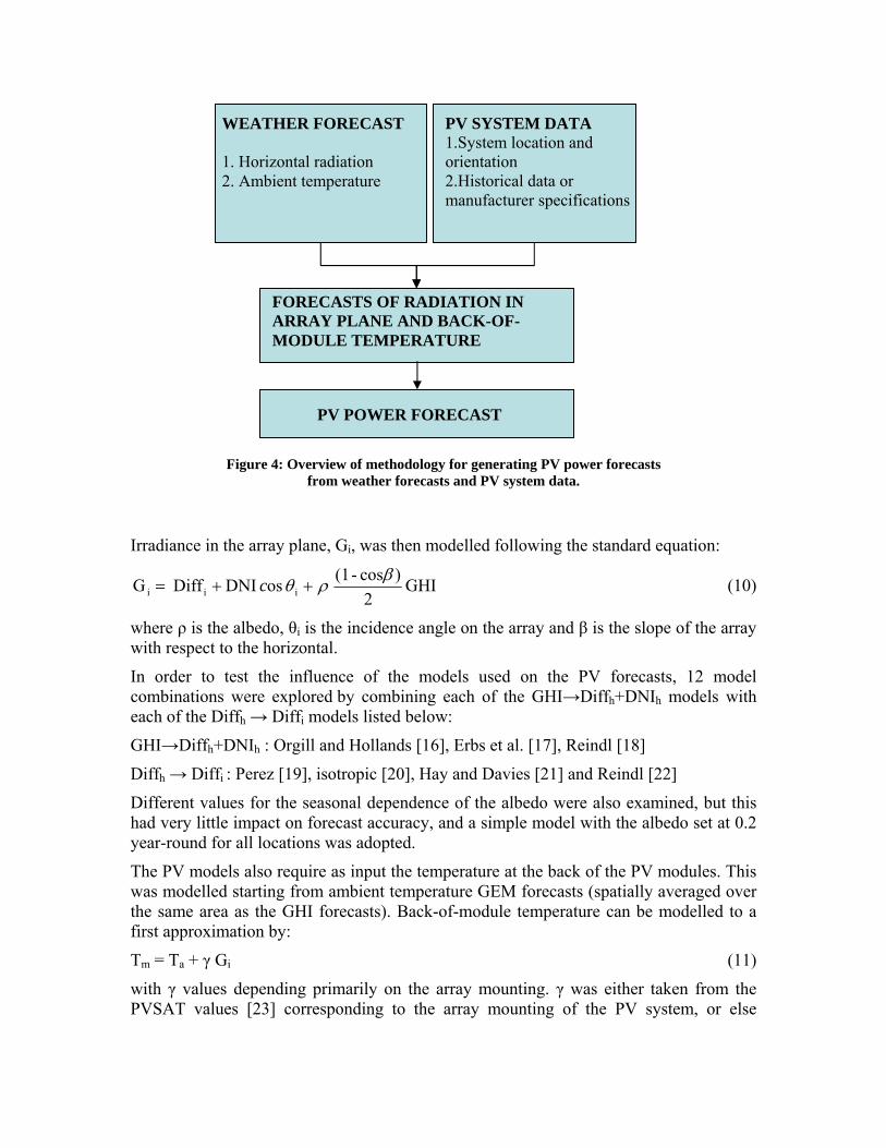
FORECASTS OF RADIATION IN ARRAY PLANE AND BACK-OF-MODULE TEMPERATURE

PV POWER FORECAST

WEATHER FORECAST 1. Horizontal radiation 2. Ambient temperature

PV SYSTEM DATA 1.System location and orientation 2.Historical data or manufacturer specifications

Figure 4: Overview of methodology for generating PV power forecasts from weather forecasts and PV system data.

Irradiance in the array plane, Gi, was then modelled following the standard equation:

GHI 2

)cos-(1 os DNI Diff G iii

c (10)

where ρ is the albedo, θi is the incidence angle on the array and β is the slope of the array with respect to the horizontal.

In order to test the influence of the models used on the PV forecasts, 12 model combinations were explored by combining each of the GHI→Diffh+DNIh models with each of the Diffh → Diffi models listed below:

GHI→Diffh+DNIh : Orgill and Hollands [16], Erbs et al. [17], Reindl [18]

Diffh → Diffi : Perez [19], isotropic [20], Hay and Davies [21] and Reindl [22]

Different values for the seasonal dependence of the albedo were also examined, but this had very little impact on forecast accuracy, and a simple model with the albedo set at 0.2 year-round for all locations was adopted.

The PV models also require as input the temperature at the back of the PV modules. This was modelled starting from ambient temperature GEM forecasts (spatially averaged over the same area as the GHI forecasts). Back-of-module temperature can be modelled to a first approximation by:

Tm = Ta + γ Gi (11)

with γ values depending primarily on the array mounting. γ was either taken from the PVSAT values [23] corresponding to the array mounting of the PV system, or else

modelled directly from PV system data (Tm, Ta, Gi) when this was available and reliable during the one year training period.

Finally, the Gi and Tm forecasts4 were used to generate (hourly average) AC output power forecasts. Again, a number of different approaches were explored, of which two are presented here. The first and simplest approach only requires historical, measured AC output power data as well as basic PV system information, namely array orientation (azimuth and tilt), array mounting (to estimate γ in equation (11)) and module type (manufacturer and model) to estimate the dependence of (DC) output power on module temperature. AC output power PAC in this first approach is simply given by:

OffsetCTP

m

WG

DerateP mDCstci

AC 2511000

,

2

for Gi>0 or θi <90° (12a)

nightACAC PP , for Gi≤0 or θi ≥90° (12b)

where equation (12a) applies to daylight hours, while (12b) simply equates AC power during nighttime hours of the test period to the average nighttime AC « output » during the training period (this is typically 0 or slightly negative). In equation (12a), α is the DC power temperature coefficient which was extracted from the data when available and taken from manufacturer specifications when it was not. The Derate and Offset coefficients were obtained by doing a linear fit of equation (12a) during the training period using measured PAC on the left-hand side and forecasted Gi and Tm on the right-hand side. In addition, the size of the region over which the GHI forecasts were averaged was varied to minimize the RMSE of the AC power forecasts during the training period. In what follows, the approach described by equations (12a) and (12b) will be referred to as the linear model.

The second approach considered here is the PVSAT approach employed by Lorenz et al. [2], trained using historical data. This could only be applied to the Varennes and Queen’s systems, since no Gi measurements were available at Exhibition Place. In this approach, the DC power for daytime hours is given by:

PDC = Gi (A + BGi + C ln Gi) (1 + D (Tm-25°C)) (13)

(Note : For nighttime hours, equation (12b) was used instead as in the first approach).

The parameters A, B, C and D were obtained by fitting equation (13) to measured PDC vs. Gi, Tm data over the training period, for hours with array incidence angles less than 60°. AC power was modelled as linear in DC power with measurements used to find the linear fit parameters.

DC power forecasts were then obtained using equation (13) with Gi and Tm forecasts as inputs and converted to AC power forecasts using the linear fit parameters identified during the training period. In order to account for calibration issues with pyranometers at Queen’s, the Gi forecasts were scaled with a scale chosen to minimize PV forecast RMSE

4 As explained in Section 4.2.1, the Erbs with Hay and Davies transposition model was used to generate the Gi forecasts.

during the training period. As in the first approach, the size of the region used for spatial averaging was tuned to minimize RMSE during the training period.

3.3.2 PV forecast benchmarking

As in the case of the irradiance forecasts, the PV forecasts were benchmarked against simpler reference models to determine the skill of the forecasts developed in this project:

Persistence: The first reference model is a simple persistence model. Following Lorenz et al. [2], PV power persistence forecasts for a given time of day h were simply obtained by setting the forecasted power equal to the most recent measured value of PV power at time h prior to the forecast (24 or 48 hours prior, depending on the forecast horizon).

GEM1: The second reference model was given by using the same approach as in 3.3.1 but without any spatial averaging, i.e. using nearest neighbour irradiance and temperature forecasts from the GEM high resolution regional grid.

The distribution of the PV forecast errors was examined to determine the frequency of occurrence of different error intervals (0 to ±5%, ±5% to ±10%, … ±95% to ±100% of rated power). Forecast errors were also compiled by month, hour of the day and forecast horizon to look for trends in the errors.

4. RESULTS AND DISCUSSION

4.1 Solar forecasts

As shown in Figure 5, both the « raw » nearest neighbour output of the GEM model and the two methods based on spatial averaging and bias removal clearly outperform the trivial persistence forecast over the 48 hour forecast period. The two methods that include spatial averaging also show a notable drop in RMSE as compared to nearest neighbour GEM forecasts. The GEM2 forecasts developed here lead to a 43% decrease in RMSE on average (skill score=0.67) when compared to the persistence forecast and to a 15% decrease in RMSE on average (skill score=0.28) when compared to the GEM1 (nearest neighbour) forecast.

0

10

20

30

40

50

60

70

Bondv

ille

Fort P

eck

Sioux F

alls

Penn

State

U.

Boulde

r

Goodw

in Cre

ek

Desert

Rock

Egber

t

Bratt's

Lake

Varenn

es

Region

Station or region

RM

SE

(%

of

mea

n)

Persistence

GEM1

Lorenz et al.

GEM2

Figure 5: Benchmarking of four solar forecast models showing RMSE as a percent of the mean

irradiance for 10 ground stations and for the average irradiance of the 10 stations (labelled “Region”).

Moreover, a recent solar forecast benchmarking exercise evaluating 7 forecast models against SURFRAD ground station data in the U.S. also found that the spatially averaged GEM forecasts lead to substantially lower RMSE’s than most of the models evaluated [24], with the exception of the ECMWF-Lorenz et al. forecasts [2] which performed comparably. This is consistent with the findings of the benchmarking exercises in Europe [5] which showed that solar forecasts from post-processing of global numerical weather prediction models performed best over forecast horizons of 1 or more days ahead.

As indicated in Table 2, RMSE reduction from bias removal is limited at the level of individual stations, since for these the bias tends to be small relative to the overall RMSE. However, in the case of stations where the bias is fairly significant (ex: the Penn State University station) bias removal can significantly reduce RMSE.

Table 2: Accuracy of global horizontal irradiance forecasts as a percentage of the average irradiance for the 10 individual ground stations and for the average irradiance of the 10 stations (denoted by

“Region”). Results are shown for the nearest neighbour GEM1 forecast, for the GEM1 avg forecast which includes spatial averaging, and for the GEM2 and Lorenz et al. forecasts which also include

bias removal.

Station Avg. GHI

(W/m2)

RMSE (%)

GEM1

RMSE (%)

GEM1 avg

RMSE (%)

Lorenz et al.

RMSE (%)

GEM2

Bias (%)

GEM1

Bias (%)

GEM1 avg

Bias (%)

Lorenz et al.

Bias (%)

GEM2

Bondville 369 32.5 28.4 29.0 27.9 5.97 5.37 -0.81 -0.26 Fort Peck 350 30.8 26.8 27.2 26.2 3.87 3.13 -0.42 -0.44 Sioux Falls 356 34.1 29.2 28.7 28.2 7.24 6.52 -0.60 -0.50 Penn State University 326 43.6 38.2 36.8 35.0 14.05 13.81 -0.50 0.07

Boulder 402 34.4 31.8 31.3 30.4 10.97 7.62 0.62 -0.52 Goodwin Creek 386 36.1 32.3 32.5 31.4 8.05 7.83 -0.38 -0.34

Desert Rock 492 16.7 16.1 16.8 16.8 1.11 1.03 0.41 -0.14

Egbert 325 38.8 34.8 34.4 33.6 7.13 7.51 0.41 0.67 Bratt's Lake 324 35.6 30.6 30.1 29.5 -0.27 0.47 -0.71 -0.40

Varennes 308 39.8 32.6 33.7 32.6 4.81 0.97 0.43 0.58 Region 476 11.4 10.0 8.8 8.8 5.57 4.81 -0.81 0

At the level of individual stations, bias removal based on a Kalman filter outperforms the Lorenz et al. approach [2] as implemented here. Meanwhile, for the « regional » forecast where the average GHI for the 10 stations is forecasted, both bias removal approaches had skill with respect to spatial averaging only, and lead to a significant reduction in RMSE. Again, this is linked to the fact that the RMSE for the regional forecast is much smaller (by about 67%) than for individual stations, so that the bias makes a relatively greater contribution to the RMSE. It is also worth nothing that the ratio of 0.33 between the regional RMSE and the average RMSE for the individual stations is what we would expect when averaging forecast errors that are uncorrelated but of similar magnitude over ten stations, namely an RMSE reduction of about 1/sqrt(10) ~0.32.

4.2 Photovoltaic forecast

4.2.1 Impact of transposition model and PV model selection

As described in 3.3.1, 12 different model combinations for generating forecasts of irradiance in the plane of the arrays from GHI forecasts were tested, as well as two different models of PV power dependence on in-plane irradiance and back-of-module temperature. The choice of the GHI → Gi transposition model had little impact on the PV forecast accuracy, as indicated by the results of Table 3. RMSE in particular is not affected much by model selection, presumably because the largest errors (that contribute

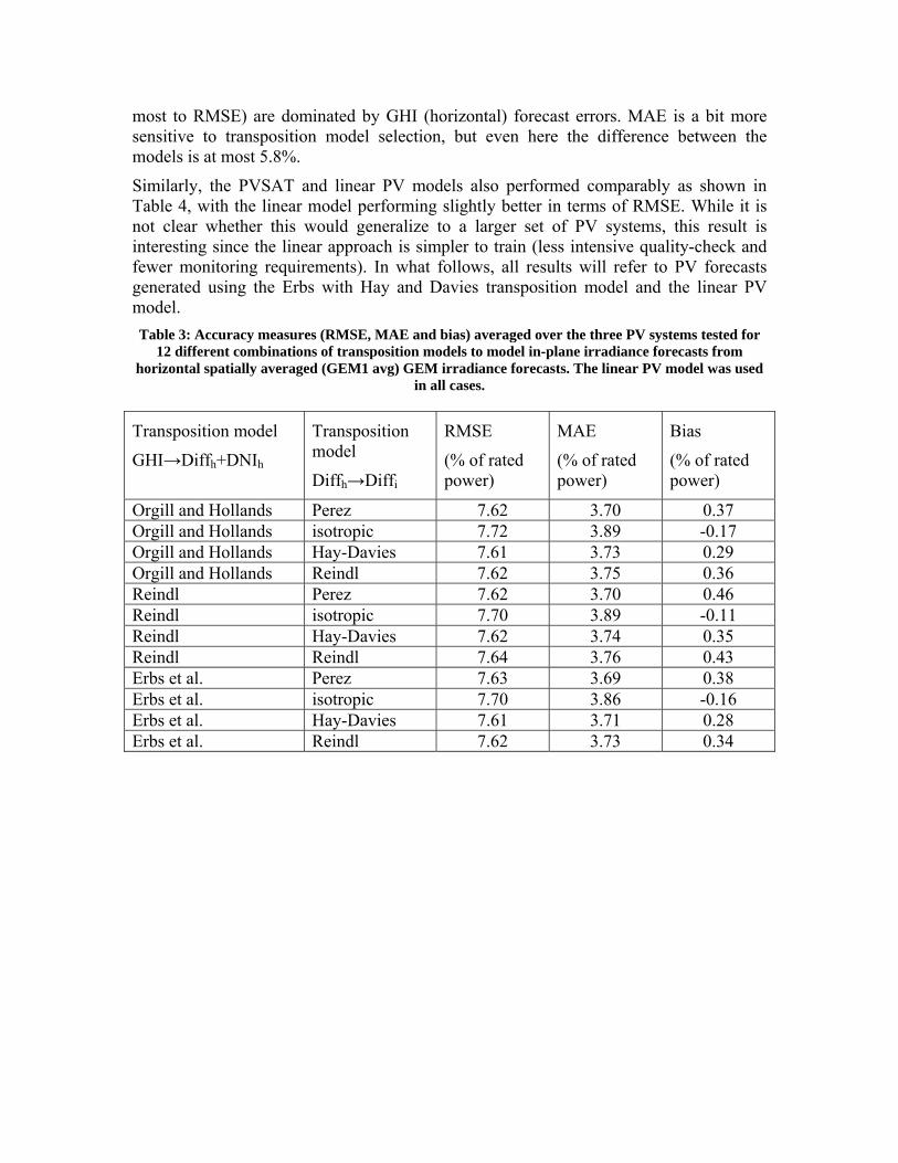
most to RMSE) are dominated by GHI (horizontal) forecast errors. MAE is a bit more sensitive to transposition model selection, but even here the difference between the models is at most 5.8%.

Similarly, the PVSAT and linear PV models also performed comparably as shown in Table 4, with the linear model performing slightly better in terms of RMSE. While it is not clear whether this would generalize to a larger set of PV systems, this result is interesting since the linear approach is simpler to train (less intensive quality-check and fewer monitoring requirements). In what follows, all results will refer to PV forecasts generated using the Erbs with Hay and Davies transposition model and the linear PV model.

Table 3: Accuracy measures (RMSE, MAE and bias) averaged over the three PV systems tested for 12 different combinations of transposition models to model in-plane irradiance forecasts from

horizontal spatially averaged (GEM1 avg) GEM irradiance forecasts. The linear PV model was used in all cases.

Transposition model

GHI→Diffh+DNIh

Transposition model

Diffh→Diffi

RMSE

(% of rated power)

MAE

(% of rated power)

Bias

(% of rated power)

Orgill and Hollands Perez 7.62 3.70 0.37 Orgill and Hollands isotropic 7.72 3.89 -0.17 Orgill and Hollands Hay-Davies 7.61 3.73 0.29 Orgill and Hollands Reindl 7.62 3.75 0.36 Reindl Perez 7.62 3.70 0.46 Reindl isotropic 7.70 3.89 -0.11 Reindl Hay-Davies 7.62 3.74 0.35 Reindl Reindl 7.64 3.76 0.43 Erbs et al. Perez 7.63 3.69 0.38 Erbs et al. isotropic 7.70 3.86 -0.16 Erbs et al. Hay-Davies 7.61 3.71 0.28 Erbs et al. Reindl 7.62 3.73 0.34

Table 4: Accuracy of the PV forecasts as a percentage of rated power for the three PV systems, and comparison of the PVSAT and linear PV model performance for the Queen’s and Varennes PV

systems. The forecasts were generated using the spatially averaged (GEM1 avg) global horizontal irradiance forecasts and the Erbs with Hay and Davies transposition model.

PV system and PV model used

RMSE

(% of rated power)

MAE

(% of rated power)

Bias

(% of rated power)

Average AC power output (W)

Rated power (W)

(DC STC)

Varennes, linear 6.38 3.14 0.24 777 6720

Varennes, PVSAT 6.44 3.02 0.38 777 6720

Queens, linear 7.27 3.44 0.07 2253 19800

Queens, PVSAT 7.50 3.43 0.43 2253 19800

Exhibition Place, linear

9.17 4.55 0.52 5729 45600

4.2.2 PV forecast accuracy and benchmarking against reference models

Figure 6 shows the outcome of the PV forecast benchmarking: PV forecasts developed here (GEM1 avg) clearly outperform persistence forecasts and GEM1 (nearest neighbour) forecasts, with (MSE) skill scores with respect to these two reference models of 0.75 and 0.19 respectively. Therefore, only GEM1 avg forecasts are discussed in the remainder of this section. More detailed results and accuracy metrics for the GEM1 avg PV forecasts are presented in Table 4. Results are reported as percentages of the DC, STC rated power of the arrays, following previous reporting on PV and wind forecasts. As a reference, the average AC power and the rated power of each array are given so that these values can be converted to absolute values or percentages of mean AC power. The RMSE, MAE and bias as a percentage of rated power range from 6.4 to 9.2%, 3.1 to 4.6% and 0 to 0.5% respectively. To put these numbers into perspective, the average AC power output of these PV systems is of the order of 11 to 12% of the rated power. These accuracies can be compared to those obtained by Lorenz et al. [2] for roughly 380 PV systems in two control areas of Germany where they found day-ahead forecast RMSE’s in the range of 4 to 5% of rated power and biases of about 1%. Given that error reduction occurs as the number of stations and the geographical area over which they are spread increase, it is reasonable to expect comparable results for Ontario when centralized PV forecasting is implemented.

0.00

2.00

4.00

6.00

8.00

10.00

12.00

14.00

16.00

18.00

20.00

Queen's Varennes Exhibition Place

RM

SE

(%

of

rate

d p

ow

er)

Persistence

GEM1

GEM1 avg

Figure 6: Benchmarking of three PV forecast models showing RMSE as a percent of rated power for

3 Canadian PV systems.

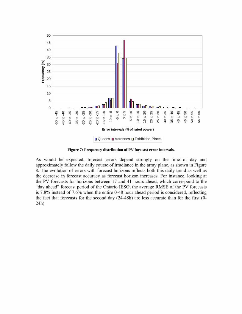
Figure 7 shows the frequency distribution of errors for the PV systems. For each system, about 76% of the errors are within ±5% of rated power (partly because of the inclusion of nighttime errors). However, the largest errors reach up to 44 to 57% of rated power. For all three systems, a majority of the largest errors is associated with over-forecasting, even though errors are fairly evenly distributed into over-forecasting and under-forecasting as a whole. For the Exhibition Place array, the largest errors come from over-forecasting in winter due to failing to account for snow cover on the arrays. For the Varennes and Queens arrays, the largest errors tend to be associated either with variable cloud situations or with overcast days where forecasts significantly underestimated cloud cover.

0

5

10

15

20

25

30

35

40

45

50

-5

0 to

-4

5

-4

5 to

-4

0

-4

0 to

-3

5

-3

5 to

-3

0

-3

0 to

-2

5

-2

5 to

-2

0

-2

0 to

-1

5

-1

5 to

-1

0

-1

0 to

-5

-5

to 0

0 to

5

5 to

10

10

to 1

5

15

to 2

0

20

to 2

5

25

to 3

0

30

to 3

5

35

to 4

0

40

to 4

5

45

to 5

0

50

to 5

5

55

to 6

0

Error intervals (% of rated power)

Fre

qu

en

cy

(%

)

Queens Varennes Exhibition Place

Figure 7: Frequency distribution of PV forecast error intervals.

As would be expected, forecast errors depend strongly on the time of day and approximately follow the daily course of irradiance in the array plane, as shown in Figure 8. The evolution of errors with forecast horizons reflects both this daily trend as well as the decrease in forecast accuracy as forecast horizon increases. For instance, looking at the PV forecasts for horizons between 17 and 41 hours ahead, which correspond to the “day ahead” forecast period of the Ontario IESO, the average RMSE of the PV forecasts is 7.8% instead of 7.6% when the entire 0-48 hour ahead period is considered, reflecting the fact that forecasts for the second day (24-48h) are less accurate than for the first (0-24h).

0

2

4

6

8

10

12

14

16

18

20

1 3 5 7 9 11 13 15 17 19 21 23

Hour of the day

RM

SE

(%

of

rate

d p

ow

er)

Queens

Varennes

Exhibition Place

Figure 8: PV forecast accuracy as a function of time of day.

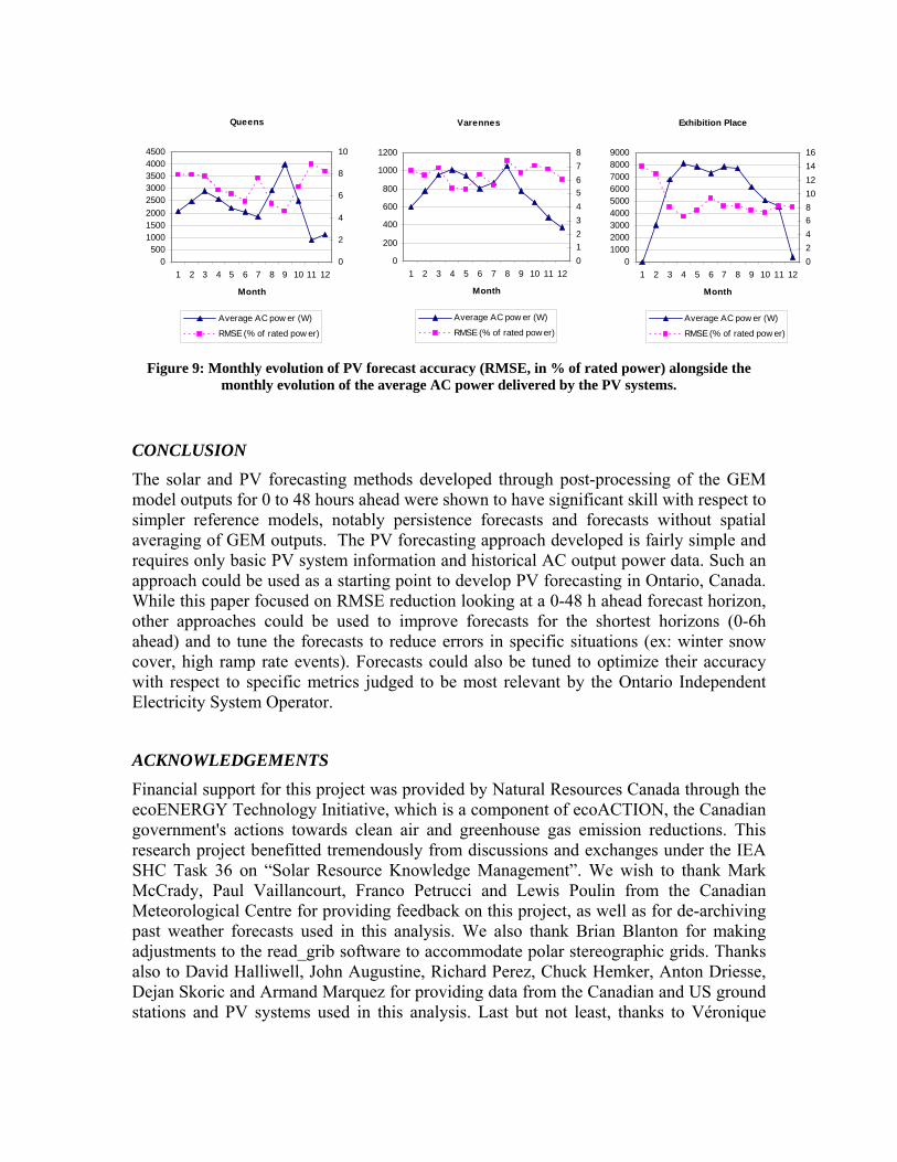
The monthly evolution of forecast accuracy was fairly system specific as can be seen in Figure 9, where monthly RMSE is shown alongside monthly average AC power for each system. Unlike the trend noted for error vs. time of day, the monthly accuracy curves do not follow the monthly average power curves for these systems. This is due in part to forecasting becoming more difficult as irradiances and solar elevations decrease. The Exhibition Place forecasts show a significant drop in accuracy during winter months, and even perform worse than the persistence forecasts in January. This is most probably due to this system’s low (20°) tilt which exacerbates issues due to snow cover and high incidence angles in the winter. In order to examine the impact of snow cover events, forecast evaluations were repeated with days flagged for snow excluded. For the Exhibition Place array, results were much better when snow cover days were excluded, with yearly RMSE dropping from 9.2% to 7.8%. This is similar to what was observed in Germany, where persistence also outperformed the forecasts being tested during months with significant snow cover [2]. However, excluding snow cover days did not substantially alter results for the Varennes and Queen’s arrays, so it’s not clear to what extent this will be an issue for PV forecasting in Ontario.

Queens

0500

100015002000

25003000350040004500

1 2 3 4 5 6 7 8 9 10 11 12

Month

0

2

4

6

8

10

Varennes

0

200

400

600

800

1000

1200

1 2 3 4 5 6 7 8 9 10 11 12

Month

0

1

2

3

4

5

6

7

8

Exhibition Place

0100020003000400050006000700080009000

1 2 3 4 5 6 7 8 9 10 11 12

Month

0

2

4

6

8

10

12

14

16

Average AC pow er (W) Average AC pow er (W)Average AC pow er (W)

Figure 9: Monthly evolution of PV forecast accuracy (RMSE, in % of rated power) alongside the monthly evolution of the average AC power delivered by the PV systems.

CONCLUSION

The solar and PV forecasting methods developed through post-processing of the GEM model outputs for 0 to 48 hours ahead were shown to have significant skill with respect to simpler reference models, notably persistence forecasts and forecasts without spatial averaging of GEM outputs. The PV forecasting approach developed is fairly simple and requires only basic PV system information and historical AC output power data. Such an approach could be used as a starting point to develop PV forecasting in Ontario, Canada. While this paper focused on RMSE reduction looking at a 0-48 h ahead forecast horizon, other approaches could be used to improve forecasts for the shortest horizons (0-6h ahead) and to tune the forecasts to reduce errors in specific situations (ex: winter snow cover, high ramp rate events). Forecasts could also be tuned to optimize their accuracy with respect to specific metrics judged to be most relevant by the Ontario Independent Electricity System Operator.

ACKNOWLEDGEMENTS

Financial support for this project was provided by Natural Resources Canada through the ecoENERGY Technology Initiative, which is a component of ecoACTION, the Canadian government's actions towards clean air and greenhouse gas emission reductions. This research project benefitted tremendously from discussions and exchanges under the IEA SHC Task 36 on “Solar Resource Knowledge Management”. We wish to thank Mark McCrady, Paul Vaillancourt, Franco Petrucci and Lewis Poulin from the Canadian Meteorological Centre for providing feedback on this project, as well as for de-archiving past weather forecasts used in this analysis. We also thank Brian Blanton for making adjustments to the read_grib software to accommodate polar stereographic grids. Thanks also to David Halliwell, John Augustine, Richard Perez, Chuck Hemker, Anton Driesse, Dejan Skoric and Armand Marquez for providing data from the Canadian and US ground stations and PV systems used in this analysis. Last but not least, thanks to Véronique

RMSE (% of rated pow er) RMSE (% of rated pow er) RMSE (% of rated pow er)

Delisle and Radu Platon for guidance on neural networks and Model Output Statistics, which were explored during trials of post-processing methods.

REFERENCES

[1] Ontario Power Authority Feed-In Tariff website, http://fit.powerauthority.on.ca/ (February 23, 2011).

[2] Lorenz E, Scheidsteger T, Hurka J, Heinemann D and Kurz C. Regional PV power prediction for improved grid integration. Prog Photovolt Res Appl 2010; n/a

doi: 10.1002/pip.1033.

[3] Lorenz E, Hurka J, Heinemann D, Beyer HG. Irradiance forecasting for the power prediction of grid-connected photovoltaic systems. IEEE Journal of Selected Topics in Applied Earth Observations and Remote Sensing 2009; 2 (1), pp. 2-10, doi:10.1109/JSTARS.2009.2020300.

[4] Focken U, Lange M, Mönnich K, Waldl HP, Beyer HG and Luig A. Short-term prediction of the aggregated power output of wind farms ─ a statistical analysis of the reduction of the prediction error by spatial smoothing effects. J. Wind Eng. Ind. Aerodyn. 2002; 90, pp. 231-246.

[5] Lorenz E, Remund J, Müller SC, Traunmüller W, Steinmaurer G, Pozo D, Ruiz-Arias JA, Lara Fanego V, Ramirez L, Romeo MG, Kurz C, Pomares LM, Guerrero CG. Benchmarking of Different Approaches to Forecast Solar Irradiance. Proceedings of the 24th European Photovoltaic Solar Energy Conference 2009; Hamburg, Germany: pp. 4199 – 4208, doi:10.4229/24thEUPVSEC2009-5BV.2.50. [6]Mailhot J, Bélair S, Lefaivre L, Bilodeau B, Desgagné M, Girard C, Glazer A, Leduc AM, Méthot A, Patoine A, Plante A, Rahill A, Robinson T, Talbot D, Tremblay A,Vaillancourt PA and Zadra A. The 15-km version of the Canadian regional forecast system. Atmosphere-Ocean 2006; 44, pp. 133-149.

[7] Environment Canada weather office website, http://www.weatheroffice.gc.ca/grib/index_e.html, (February 23, 2011).

[8] Read_grib open source program, http://workhorse.europa.renci.org/~bblanton/ReadGrib/, (February 23, 2011).

[9] National Oceanic and Atmospheric Administration website, SURFRAD (Surface Radiation) Network, http://www.srrb.noaa.gov/surfrad/, (February 23, 2011).

[10] Hoyer-Klick C, Beyer HG, Dumortier D, Schroedter-Homscheidt M, Wald L, MartinoliM, Schilings C, Gschwind B, Menard L, Gaboardi E, Ramirez-Santigosa L, Polo J, Cebecauer T, Huld T, Suri M, de Blas M, Lorenz E, Pfatischer R, Remund J, Ineichen P, Tsvetkov A, Hofierka J. Management and Exploitation of Solar Resource Knowledge. Proceedings of Eurosun 2008; Lisbon, Portugal.

[11] Environment Canada National Climate Data and Information Archive, http://climate.weatheroffice.gc.ca/climateData/canada_e.html, (February 23, 2011).

[12] Beyer HG, Polo Martinez J, Suri M, Torres JL, Lorenz E, Müller SC, Hoyer-Klick C and Ineichen P. D 1.1.3 Report on Benchmarking of Radiation Products. Report under contract no. 038665 of MESoR, available for download at http://www.mesor.net/deliverables.html, (February 23, 2011).

[13] Louka P, Galanis G, Siebert N, Kariniotakis G, Katsafados P, Pytharoulis I and Kallos G. Improvements in wind speed forecasts for wind power prediction purposes using Kalman filtering. Journal of Wind Engineering and Industrial Aerodynamics 2008; 96, pp. 2348-2362.

[14] Galanis G, Louka P, Katsafados P, Kallos G and Pytharoulis I. Applications of Kalman filters based on non-linear functions to numerical weather predictions. Ann. Geophys. 2006; 24, pp. 2451-2460.

[15] Rigollier C, Bauer O and Wald L. On the clear sky model of the ESRA ─ European Solar Radiation Atlas ─ With respect to the Heliosat method. Solar Energy 2000; 68 (1), pp. 33-48.

[16] Orgill JF and Hollands KGT. Correlation Equation for Hourly Diffuse Radiation on a Horizontal Surface. Solar Energy 1977; 19 (4), pp. 357-359.

[17] Erbs DG, Klein SA and Duffie JA. Estimation of the diffuse radiation fraction for hourly, daily and monthly-average global radiation. Solar Energy 1982; 28 (4), pp. 293-302.

[18] Reindl DT, Beckman WA and Duffie JA, Diffuse Fraction Correlations, Solar Energy 1990; 45 (1), pp.1-7.

[19] Perez R, Ineichen P, Seals R, Michalsky J and Stewart R. Modeling daylight availability and irradiance components from direct and global irradiance. Solar Energy 1990; 44 (5), pp.271-289, doi:10.1016/0038-092X(90)90055-H.

[20] Duffie JA and Beckman WA. Solar Engineering of Thermal Processes. Wiley: New York, 1991; pp. 94-95.

[21] Hay JE and Davies JA, Calculation of the Solar Radiation Incident on an Inclined Surface, Proceedings First Canadian Solar Radiation Workshop 1980, pp. 59-72.

[22] Reindl DT, Beckman WA and Duffie JA. Evaluation of Hourly Tilted Surface Radiation Models. Solar Energy 1990; 45 (1), pp. 9-17.

[23] Drews A, de Keizer AC, Beyer HG, Lorenz E, Betcke J, van Sark WGJHM, Heydenreich W, Wiemken E, Stettler S, Toggweiler P, Bofinger S, Schneider M, Heilscher G, Heinemann D. Monitoring and remote failure detection of grid-connected PV systems based on satellite observations. Solar Energy 2007; 81 (4), pp. 548-564, doi:10.1016/j.solener.2006.06.019. [24] Perez R, Beauharnois M, Hemker K, Kivalov S, Lorenz E, Pelland S, Schlemmer J, Van Knowe G. Evaluation of Numerical Weather Prediction solar irradiance forecasts in the US. In preparation (to be presented at the 2011 ASES Annual Conference).