solar and photovoltaic forecasting through post...

PROGRESS IN PHOTOVOLTAICS: RESEARCH AND APPLICATIONSProg. Photovolt: Res. Appl. (2011)

Published online in Wiley Online Library (wileyonlinelibrary.com). DOI: 10.1002/pip.1180

RESEARCH ARTICLE

Solar and photovoltaic forecasting throughpost-processing of the Global EnvironmentalMultiscale numerical weather prediction modelSophie Pelland1*, George Galanis2,3 and George Kallos2

1 CanmetENERGY, Natural Resources Canada, Varennes, Québec, Canada2 Atmospheric Modeling and Weather Forecasting Group, Department of Physics, University of Athens, Athens, Greece3 Section of Mathematics, Naval Academy of Greece, Piraeus, Greece

ABSTRACT

Hourly solar and photovoltaic (PV) forecasts for horizons between 0 and 48 h ahead were developed using EnvironmentCanada’s Global Environmental Multiscale model. The motivation for this research was to explore PV forecasting inOntario, Canada, where feed-in tariffs are driving rapid growth in installed PV capacity. The solar and PV forecasts werecompared with irradiance data from 10 North-American ground stations and with alternating current power data from threeCanadian PV systems. A 1-year period was used to train the forecasts, and the following year was used for testing. Twopost-processing methods were applied to the solar forecasts: spatial averaging and bias removal using a Kalman filter.On average, these two methods lead to a 43% reduction in root mean square error (RMSE) over a persistence forecast (skillscore = 0.67) and to a 15% reduction in RMSE over the Global Environmental Multiscale forecasts without post-processing(skill score = 0.28). Bias removal was primarily useful when considering a “regional” forecast for the average irradiance ofthe 10 ground stations because bias was a more significant fraction of RMSE in this case. PV forecast accuracy wasinfluenced mainly by the underlying (horizontal) solar forecast accuracy, with RMSE ranging from 6.4% to 9.2% of ratedpower for the individual PV systems. About 76% of the PV forecast errors were within�5% of the rated power for theindividual systems, but the largest errors reached up to 44% to 57% of rated power. © Her Majesty the Queen in Right of Canada2011. Reproduced with the permission of the Minister of Natural Resources Canada.

KEYWORDS

solar forecasting; photovoltaic forecasting; numerical weather prediction; post-processing; Kalman filter; spatial averaging

*Correspondence

Sophie Pelland, CanmetENERGY, Natural Resources Canada, Varennes, Québec, CanadaE-mail: [email protected]

Received 20 April 2011; Revised 12 July 2011; Accepted 11 August 2011

1. INTRODUCTION

In order to integrate large amounts of intermittent renew-able generation reliably and cost-effectively into electric-ity grids, system operators need both to understand thevariability of these generators and to be able to forecastthis variability at different spatial and temporal scales. Al-though the timescales relevant for forecasting vary, mostsystem operators use a day-ahead commitment processto commit generators to meet the next day’s forecastedload. Moving closer to real time, updated conditions andforecasts are used to dispatch generators, secure reserves,and lock in imports and exports. Meanwhile, the geo-graphic area of interest for forecasting can vary from a largearea over which electricity supply and demand must be

© Her Majesty the Queen in Right of Canada 2011. Reproduced with the perm

balanced to a much smaller region where grid congestionmust be managed.

The motivation for the research presented here was the in-troduction of feed-in tariffs in the province of Ontario,Canada [1], which led to a rapid increase in the contractedand installed capacity of photovoltaics (PV) and other renew-ables in Ontario. The Ontario Independent Electricity SystemOperator (IESO) recently put forward a call for proposals todevelop centralized wind forecasting for the province, whichhas an installed wind capacity of over 1.1GW and a peakload of about 27GW. Meanwhile, contracts for over 1GWof PV systems have been offered under the Feed-In TariffProgram [1], and PV forecasting implementation shouldbegin once installed PV capacity becomes comparable withthe (current) installed wind capacity.

ission of the Minister of Natural Resources Canada.

Solar and photovoltaic forecasting S. Pelland, G. Galanis and G. Kallos

Although many system operators around the worldhave implemented wind forecasting, solar forecasting iscomparatively recent. One interesting implementation istaking place in Germany: at the end of 2008, two Germantransmission system operators with (at the time) 2.9GW ofinstalled PV corresponding to over 200,000 systems acrosstheir balancing areas mandated different forecast providersto implement and test PV forecasts for their balancingareas. The University of Oldenburg and MeteocontrolGmbH have reported results from their ongoing forecastevaluations in [2]. As in the case of wind forecasting,research from the University of Oldenburg shows that solarand PV forecast accuracy improves significantly as the sizeof the geographic area under consideration increases, witha reduction in root mean square error (RMSE) of about64% for a forecast over an area the size of Germany as com-pared with a point forecast [3]. This effect was modeled indetail by Focken et al. [4] in the case of wind: they showedthat both the size of the geographic area and the numberof stations or systems considered contributed to error re-duction, with the reduction from an increased number ofstations saturating beyond a certain threshold for a givengeographic area. For both PV and wind forecasting, themost appropriate approach depends on the forecast horizon:for forecast horizons of about 0 to 6 h ahead, methods basedprimarily on observations (from ground stations or satel-lites) tend to perform best, whereas for forecast horizonsof about 6 h to a few days ahead, global numerical weatherprediction models become more accurate [5].

The approach described in this paper focuses on 0–48-h-ahead forecasts based on post-processing of a globalnumerical weather prediction model, namely EnvironmentCanada’s Global Environmental Multiscale (GEM) model.The GEM forecasts and the solar and PV data used forcomparisons are described in Section 2, along with thequality check procedures that were applied to the data.Section 3 presents the post-processing (spatial averagingand Kalman filter) that was performed to improve theforecast accuracy. Section 4 examines the accuracy of theforecasts and the distribution of forecast errors, as well asthe increase in forecast skill through post-processing; thisis followed by concluding comments in Section 5.

1Also, forecasts originating at 6 and 18 UTC were not available atthe beginning of the 2-year period considered. Meanwhile, pre-liminary tests comparing the 0 and 12 UTC forecasts indicatedthat the RMSEs are lower for the 12 UTC forecasts.

2. SOLAR FORECASTS AND DATAUSED FOR FORECAST EVALUATION

2.1. GEM weather forecasts

Environment Canada’s Canadian Meteorological Centreoperates a global numerical weather prediction modelknown as the GEM model [6]. The model is run in differ-ent configurations, including a configuration known as the“high-resolution regional run,” which generates forecastsfor horizons between 0 and 48 h ahead at a 7.5-min timestep over a variable spatial resolution grid, with a spatialresolution reaching about 15 km at the grid center, inCanada. Model runs are initiated up to four times a day,

Prog. Photovolt: Res. Appl. (2011) ©HerMajesty theQueen inRight of Canada 201

at 0 UTC, 6 UTC, 12 UTC, and 18 UTC, and a subset ofmodel outputs is made available online at time steps of3 h or more [7]. For the purpose of this analysis, theCanadian Meteorological Centre de-archived past forecastsfrom the high-resolution regional run at an hourly time stepover the 2-year period between 1 April 2007 and 31 March2009 for several weather variables, including downwardshortwave radiation flux (DSWRF) at the surface, temper-ature at 2m above the surface, and total cloud cover(TCDC) [7]. The de-archived forecasts cover NorthAmerica and adjacent waters.

Only forecasts originating at 12 UTC were consideredhere because these are the most relevant for day-ahead PVforecasting in Ontario: currently, generators (of 20MW ormore) are asked by the Ontario IESO to produce forecastsby 11AM for each hour of the following day, which meansthat 12 UTC (7AM EST in Ontario) forecasts are the mostrecent forecasts available prior to the 11AM deadline.1 Theday-ahead IESO forecast period corresponds to forecasthorizons of 17 to 41 h ahead in the GEM 12 UTC forecast.Forecasts were provided in Grib1 format and wereextracted for the variables and grid points of interest usingthe open-source program read_grib [8] in MATLAB.

2.2. Ground station irradiance data and dataquality check procedure

The stations shown on the map in Figure 1 were selectedto test the accuracy of the GEM regional solar forecasts.In Canada, the three stations selected measure direct, skydiffuse, and global horizontal irradiance (GHI) eachsecond, with 1-min averages and standard deviations beingrecorded. GHI is measured with Kipp & Zonen CMP 21(Delft, the Netherlands) pyranometers; these are high-quality instruments according to the World MeteorologicalOrganization ratings, with achievable uncertainties (at the95% confidence level) of 3% for hourly totals [9]. Thethree Canadian stations are operated by EnvironmentCanada and by Natural Resources Canada, with stationsbeing maintained on a daily basis and pyranometerscalibrated every 2 years. Similarly, the seven US stationsselected measure global horizontal, sky diffuse, and directirradiance every 3min up to January 2009 and everyminute after that. GHI is measured using Eppley PSP(Eppley Laboratory, Newport, RI, USA) pyranometers thatare calibrated once a year; these conform to the sameperformance standards listed above for the Kipp & ZonenCMP 21s. The seven US stations comprise the US SurfaceRadiation Budget network [10]. Along with the station atBratt’s Lake, these are part of the Baseline SurfaceRadiation Network, a worldwide network of research-grade radiation measurement stations.

1.Reproducedwith the permission of theMinister ofNatural ResourcesCanada.DOI: 10.1002/pip

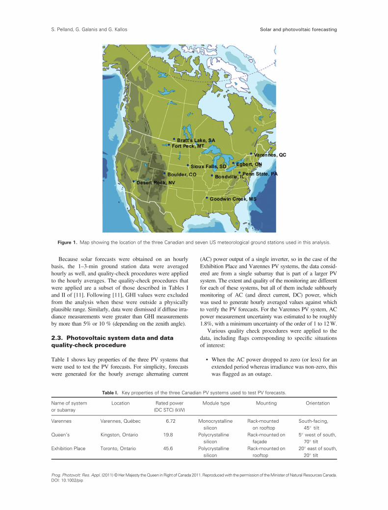
Figure 1. Map showing the location of the three Canadian and seven US meteorological ground stations used in this analysis.

Solar and photovoltaic forecastingS. Pelland, G. Galanis and G. Kallos

Because solar forecasts were obtained on an hourlybasis, the 1–3-min ground station data were averagedhourly as well, and quality-check procedures were appliedto the hourly averages. The quality-check procedures thatwere applied are a subset of those described in Tables Iand II of [11]. Following [11], GHI values were excludedfrom the analysis when these were outside a physicallyplausible range. Similarly, data were dismissed if diffuse irra-diance measurements were greater than GHI measurementsby more than 5% or 10 % (depending on the zenith angle).

2.3. Photovoltaic system data and dataquality-check procedure

Table I shows key properties of the three PV systems thatwere used to test the PV forecasts. For simplicity, forecastswere generated for the hourly average alternating current

Table I. Key properties of the three Canadia

Name of systemor subarray

Location Rated power(DC STC) (kW)

Varennes Varennes, Québec 6.72 M

Queen’s Kingston, Ontario 19.8 P

Exhibition Place Toronto, Ontario 45.6 P

Prog. Photovolt: Res. Appl. (2011) ©HerMajesty theQueen inRight of Canada 201DOI: 10.1002/pip

(AC) power output of a single inverter, so in the case of theExhibition Place and Varennes PV systems, the data consid-ered are from a single subarray that is part of a larger PVsystem. The extent and quality of the monitoring are differentfor each of these systems, but all of them include subhourlymonitoring of AC (and direct current, DC) power, whichwas used to generate hourly averaged values against whichto verify the PV forecasts. For the Varennes PV system, ACpower measurement uncertainty was estimated to be roughly1.8%, with a minimum uncertainty of the order of 1 to 12W.

Various quality check procedures were applied to thedata, including flags corresponding to specific situationsof interest:

• When the AC power dropped to zero (or less) for anextended period whereas irradiance was non-zero, thiswas flagged as an outage.

n PV systems used to test PV forecasts.

Module type Mounting Orientation

onocrystallinesilicon

Rack-mountedon rooftop

South-facing,45� tilt

olycrystallinesilicon

Rack-mounted onfaçade

5� west of south,70� tilt

olycrystallinesilicon

Rack-mounted onrooftop

20� east of south,20� tilt

1. Reproducedwith the permission of theMinister ofNatural ResourcesCanada.


• Using Environment Canada’s Climate Data Online[12], days surrounding significant snowfall events atthe ground station nearest to each PV system weresingled out for further study. Visual inspection ofthe data was used to assign a tentative snow coverflag, with snow cover being flagged when a noticeabledrop in the daily performance ratio coincided withsnowfall.

Days flagged for snow cover were included in thetesting period, but the snow flags were used to determinethe impact of these events on forecast accuracy. Meanwhile,outages were excluded from the PV forecast evaluation toreflect the expectation that outages for well-monitoredmegawatt-scale systems or over ensembles of smallerindependent systems should be quite rare and taken intoaccount in the forecasting process when they do occur.

3. SOLAR AND PHOTOVOLTAICFORECAST DEVELOPMENT ANDTESTING

3.1. Forecast accuracy measures

The accuracy measures used to evaluate load, wind, andsolar forecasts vary. Along with variations in forecastaccuracy depending on the region, forecast horizon, andevaluation period, this makes comparisons between fore-casting methods challenging. Benchmarking of solarforecasts has been examined by the International EnergyAgency Solar Heating and Cooling Program Task 36 on“Solar Resource Knowledge Management” and its sisterproject “Management and Exploitation of Solar ResourceKnowledge,” which have suggested guidelines for bench-marking and conducted comparisons of different solarforecast models against sets of common ground stationdata [5,13]. Following [13], solar and PV forecast accuracywas assessed in terms of RMSE, mean absolute error(MAE), and mean bias error (bias), which are definedhere as

RMSE ¼ffiffiffiffiffiffiffiffiffiffiMSE

p¼

ffiffiffiffiffiffiffiffiffiffiffiffiffiffiffiffiffiffiffiffiffiffiffiffiffiffiffiffiffiffiffiffiffiffiffiffiffiffiffiffiXni¼1

xpred; i � xobs; i� �2

n

vuut (1)

MBE ¼ Bias ¼Xni¼1

xpred; i � xobs; i� �

n(2)

MAE ¼Xni¼1

xpred; i � xobs; i��

n(3)

where xpred,i and xobs,i represent the ith valid forecast andobservation pair, respectively, and where the sums arecarried out over all n such pairs within the 1-year testingperiod from 1 April 2008 to 31 March 2009. Unlessstated otherwise, these accuracy measures were computed


over the entire 0- to 48-h forecast period. For solar fore-casts, evaluation was restricted to daylight hours becauseforecasting irradiance at night is trivial. Meanwhile, forPV forecasts, evaluation was conducted over all hours ofthe day because forecast operators require forecastingfrom generators at all times (and because some PV systeminverters may consume small amounts of power from thegrid at night).

As the above definitions indicate, RMSE gives moreweight to large errors, whereas MAE reveals the averagemagnitude of the error and bias indicates whether there isa significant (and corrigible) tendency to systematicallyover-forecast or under-forecast. When comparing betweendifferent models in the training year, RMSE was used asthe metric for minimization, that is, forecasts were trainedwith the goal of reducing the largest errors.

In order to facilitate comparisons, these different accu-racy measures will be quoted in this paper both in termsof absolute values and as percentages of a reference value:the mean irradiance for solar forecasts and the DC Stan-dard Test Conditions (STC) array rating for PV forecasts.Finally, as detailed in Sections 3.2.3 and 3.3.2, forecastswill also be benchmarked with respect to different refer-ence models in terms of their mean square error (MSE)skill score, which is defined as follows:

skill score ¼ MSEreference �MSEforecast

MSEreference(4)

The skill score indicates the fractional improvement inthe MSE over a reference model: a skill score of 1 indicatesa perfect forecast, a score of 0 indicates no improvementover the reference, and a negative skill means that theforecast model tested performs worse than the reference.

3.2. Post-processing and benchmarking ofthe irradiance forecasts

3.2.1. Spatial averaging.As mentioned in Section 2.1, 0–48-h-ahead forecasts ofinstantaneous DSWRF were extracted for grid pointsaround each location of interest. In order to generateforecasts of hourly averaged GHI (aka GHI or solarforecasts), we simply averaged the DSWRF forecasts at thebeginning and end of each hour. Preliminary tests revealedthat this approach yields slightly better results thancomputing the hourly averages by taking differencesbetween total accumulated DSWRF from consecutive hours.

Following Lorenz et al. [2], two types of post-processing were applied to the irradiance forecasts, namelyspatial averaging and bias removal. As noted in [13], spatialaveraging of irradiance forecasts can lead to improvedforecast accuracy by smoothing the variations due tochanging cloud cover, which are difficult to pinpoint at the~15-km scale associated with a single grid square. Spatialaveraging was tested for each of the 10 ground stations byconsidering the average of the irradiance forecasts over asquare grid centered around each station and containing



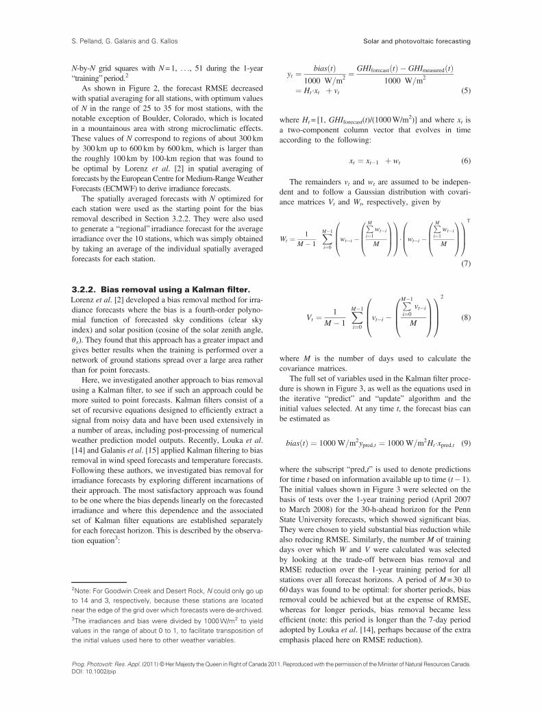
N-by-N grid squares with N=1, . . ., 51 during the 1-year“training”period.2

As shown in Figure 2, the forecast RMSE decreasedwith spatial averaging for all stations, with optimum valuesof N in the range of 25 to 35 for most stations, with thenotable exception of Boulder, Colorado, which is locatedin a mountainous area with strong microclimatic effects.These values of N correspond to regions of about 300 kmby 300 km up to 600 km by 600 km, which is larger thanthe roughly 100 km by 100-km region that was found tobe optimal by Lorenz et al. [2] in spatial averaging offorecasts by the European Centre for Medium-RangeWeatherForecasts (ECMWF) to derive irradiance forecasts.

The spatially averaged forecasts with N optimized foreach station were used as the starting point for the biasremoval described in Section 3.2.2. They were also usedto generate a “regional” irradiance forecast for the averageirradiance over the 10 stations, which was simply obtainedby taking an average of the individual spatially averagedforecasts for each station.

3.2.2. Bias removal using a Kalman filter.Lorenz et al. [2] developed a bias removal method for irra-diance forecasts where the bias is a fourth-order polyno-mial function of forecasted sky conditions (clear skyindex) and solar position (cosine of the solar zenith angle,θz). They found that this approach has a greater impact andgives better results when the training is performed over anetwork of ground stations spread over a large area ratherthan for point forecasts.

Here, we investigated another approach to bias removalusing a Kalman filter, to see if such an approach could bemore suited to point forecasts. Kalman filters consist of aset of recursive equations designed to efficiently extract asignal from noisy data and have been used extensively ina number of areas, including post-processing of numericalweather prediction model outputs. Recently, Louka et al.[14] and Galanis et al. [15] applied Kalman filtering to biasremoval in wind speed forecasts and temperature forecasts.Following these authors, we investigated bias removal forirradiance forecasts by exploring different incarnations oftheir approach. The most satisfactory approach was foundto be one where the bias depends linearly on the forecastedirradiance and where this dependence and the associatedset of Kalman filter equations are established separatelyfor each forecast horizon. This is described by the observa-tion equation3:

2Note: For Goodwin Creek and Desert Rock, N could only go upto 14 and 3, respectively, because these stations are locatednear the edge of the grid over which forecasts were de-archived.3The irradiances and bias were divided by 1000W/m2 to yieldvalues in the range of about 0 to 1, to facilitate transposition ofthe initial values used here to other weather variables.


yt ¼ bias tð Þ1000 W=m2 ¼

GHIforecast tð Þ � GHImeasured tð Þ1000 W=m2

¼ Ht �xt þ vt (5)

where Ht = [1, GHIforecast(t)/(1000W/m2)] and where xt isa two-component column vector that evolves in timeaccording to the following:

xt ¼ xt�1 þ wt (6)

The remainders vt and wt are assumed to be indepen-dent and to follow a Gaussian distribution with covari-ance matrices Vt and Wt, respectively, given by

Wt ¼ 1M � 1

XM�1

i¼0

wt�i �PMi¼1

wt�i

M

0BB@

1CCA

0BB@

1CCA� wt�i �

PMi¼1

wt�i

M

0BB@

1CCA

0BB@

1CCA

T

(7)

Vt ¼ 1M � 1

XM�1

i¼0

vt�i �PM�1

i¼0vt�i

M

0BB@

1CCA

0BB@

1CCA

2

(8)

where M is the number of days used to calculate thecovariance matrices.

The full set of variables used in the Kalman filter proce-dure is shown in Figure 3, as well as the equations used inthe iterative “predict” and “update” algorithm and theinitial values selected. At any time t, the forecast bias canbe estimated as

bias tð Þ ¼ 1000 W=m2ypred;t ¼ 1000 W=m2Ht�xpred;t (9)

where the subscript “pred,t” is used to denote predictionsfor time t based on information available up to time (t� 1).The initial values shown in Figure 3 were selected on thebasis of tests over the 1-year training period (April 2007to March 2008) for the 30-h-ahead horizon for the PennState University forecasts, which showed significant bias.They were chosen to yield substantial bias reduction whilealso reducing RMSE. Similarly, the number M of trainingdays over which W and V were calculated was selectedby looking at the trade-off between bias removal andRMSE reduction over the 1-year training period for allstations over all forecast horizons. A period of M= 30 to60 days was found to be optimal: for shorter periods, biasremoval could be achieved but at the expense of RMSE,whereas for longer periods, bias removal became lessefficient (note: this period is longer than the 7-day periodadopted by Louka et al. [14], perhaps because of the extraemphasis placed here on RMSE reduction).

1.Reproducedwith the permission of theMinister ofNatural ResourcesCanada.

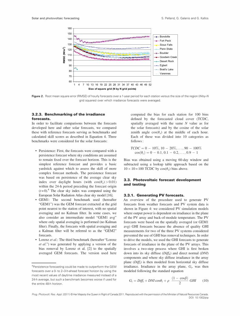
Figure 2. Root mean square error (RMSE) of hourly forecasts over a 1-year period for each station versus the size of the region (N-by-Ngrid squares) over which irradiance forecasts were averaged.


3.2.3. Benchmarking of the irradianceforecasts.In order to facilitate comparisons between the forecastsdeveloped here and other solar forecasts, we comparedthese with reference forecasts serving as benchmarks andcalculated skill scores as described in Equation 4. Threebenchmarks were considered for the solar forecasts:

• Persistence: First, the forecasts were compared with apersistence forecast where sky conditions are assumedto remain fixed over the forecast horizon. This is thesimplest reference forecast and provides a basicyardstick against which to assess the skill of morecomplex forecast methods. The persistence forecastwas based on persistence of the average clear skyindex over daylight hours (with cos(θz)> 0.01)within the 24-h period preceding the forecast origin(t=0).4 The clear sky index was computed using theEuropean Solar Radiation Atlas clear sky model [16].

• GEM1: The second benchmark used (hereafter“GEM1”) was the GEM forecast extracted at the gridpoint nearest to the station of interest, with no spatialaveraging and no Kalman filter. In some cases, wealso consider an intermediate model “GEM1 avg”where only spatial averaging is performed (no Kalmanfilter). Finally, the forecasts with spatial averaging anda Kalman filter will be referred to as the “GEM2”forecasts.

• Lorenz et al.: The third benchmark (hereafter “Lorenzet al.”) was generated by applying a version of thebias removal by Lorenz et al. [2] to the spatiallyaveraged GEM forecasts. The version used here

4Persistence forecasting could be made to outperform the GEMforecasts over a 0- to 2–3-h-ahead forecast horizon by using themost recent values of daytime irradiance measured instead of a24-h average, but such a benchmark becomes worse if used forthe entire 48-h horizon.


computed the bias for each station for 100 binsdefined by the forecasted cloud cover (TCDC,spatially averaged with the same N value as forthe solar forecasts) and by the cosine of the solarzenith angle cos(θz) at the middle of each hour.Each of these was divided into 10 categories asfollows :

TCDC ¼ 0 � 10%; 10 � 20%; . . . ; 90 � 100%cos θzð Þ ¼ 0 � 0:1; 0:1 � 0:2; . . . ; 0:9 � 1

Bias was obtained using a moving 60-day window andsubtracted using a lookup table approach based on the10� 10 = 100 TCDC by cos(θz) bins above.

3.3. Photovoltaic forecast developmentand testing

3.3.1. Generating PV forecasts.An overview of the procedure used to generate PVforecasts from weather forecasts and PV system data isshown in Figure 4: we considered PV simulation modelswhere output power is dependent on irradiance in the planeof the PV array and back-of-module temperature. The PVforecasts were based on the spatially averaged (or GEM1avg) GHI forecasts because the absence of quality GHImeasurements for two of the three PV systems consideredprevented the use of GHI bias removal techniques. In orderto drive the models, we used the GHI forecasts to generateforecasts of irradiance in the plane of the PV arrays. Thisinvolves a two-step process where GHI is first brokendown into its sky diffuse (Diffh) and direct normal (DNI)components and where sky diffuse irradiance in the arrayplane (Diffi) is then modeled from horizontal sky diffuseirradiance. Irradiance in the array plane, Gi, was thenmodeled following the standard equation

Gi ¼ Diffi þ DNI cosθi þ r1� cosbð Þ

2GHI (10)


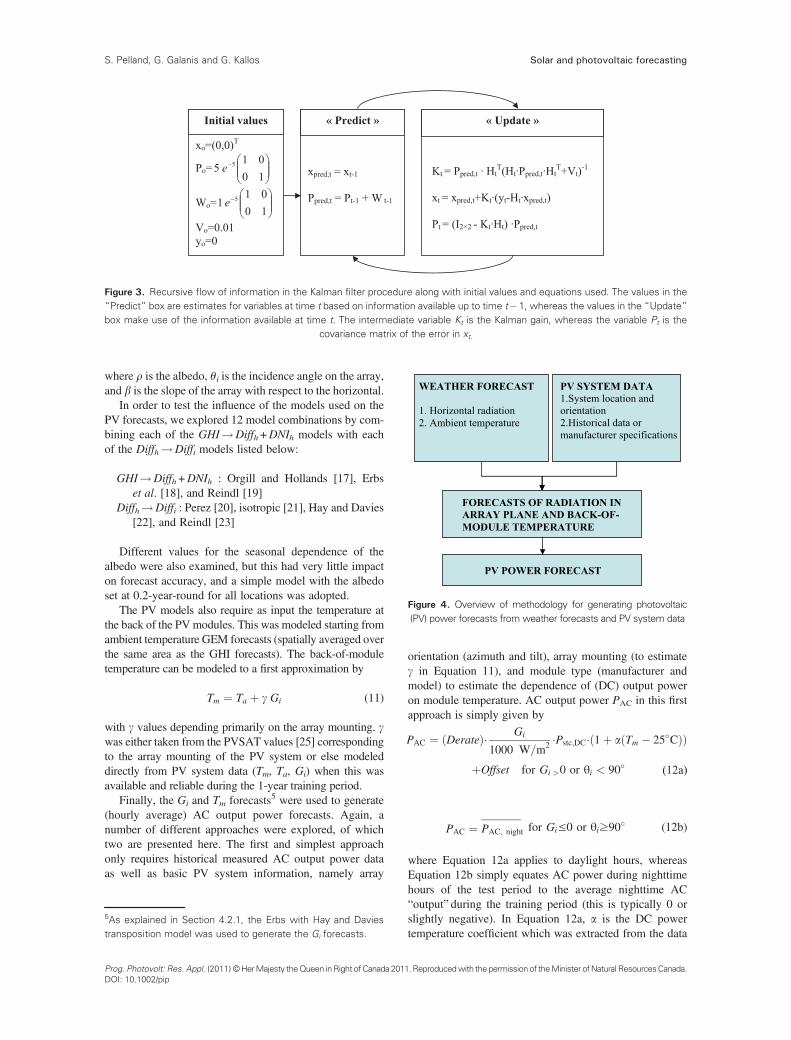
Figure 3. Recursive flow of information in the Kalman filter procedure along with initial values and equations used. The values in the“Predict” box are estimates for variables at time t based on information available up to time t� 1, whereas the values in the “Update”box make use of the information available at time t. The intermediate variable Kt is the Kalman gain, whereas the variable Pt is the

covariance matrix of the error in xt.

Figure 4. Overview of methodology for generating photovoltaic(PV) power forecasts from weather forecasts and PV system data


where r is the albedo, θi is the incidence angle on the array,and b is the slope of the array with respect to the horizontal.

In order to test the influence of the models used on thePV forecasts, we explored 12 model combinations by com-bining each of the GHI!Diffh+DNIh models with eachof the Diffh!Diffi models listed below:

GHI!Diffh+DNIh : Orgill and Hollands [17], Erbset al. [18], and Reindl [19]

Diffh!Diffi : Perez [20], isotropic [21], Hay and Davies[22], and Reindl [23]

Different values for the seasonal dependence of thealbedo were also examined, but this had very little impacton forecast accuracy, and a simple model with the albedoset at 0.2-year-round for all locations was adopted.

The PV models also require as input the temperature atthe back of the PVmodules. This was modeled starting fromambient temperature GEM forecasts (spatially averaged overthe same area as the GHI forecasts). The back-of-moduletemperature can be modeled to a first approximation by

Tm ¼ Ta þ g Gi (11)

with g values depending primarily on the array mounting. gwas either taken from the PVSAT values [25] correspondingto the array mounting of the PV system or else modeleddirectly from PV system data (Tm, Ta, Gi) when this wasavailable and reliable during the 1-year training period.

Finally, the Gi and Tm forecasts5 were used to generate(hourly average) AC output power forecasts. Again, anumber of different approaches were explored, of whichtwo are presented here. The first and simplest approachonly requires historical measured AC output power dataas well as basic PV system information, namely array

5As explained in Section 4.2.1, the Erbs with Hay and Daviestransposition model was used to generate the Gi forecasts.


orientation (azimuth and tilt), array mounting (to estimateg in Equation 11), and module type (manufacturer andmodel) to estimate the dependence of (DC) output poweron module temperature. AC output power PAC in this firstapproach is simply given by

PAC ¼ Derateð Þ� Gi

1000 W=m2 �Pstc;DC� 1þ a Tm � 25�Cð Þð Þ

þOffset for Gi >0 or θi < 90�

PAC ¼�PAC; night for Gi≤0 or θi≥90� (12b)

where Equation 12a applies to daylight hours, whereasEquation 12b simply equates AC power during nighttimehours of the test period to the average nighttime AC“output” during the training period (this is typically 0 orslightly negative). In Equation 12a, a is the DC powertemperature coefficient which was extracted from the data

(12a)



when available and taken from manufacturer specificationswhen it was not. The Derate and Offset coefficients wereobtained by doing a linear fit of Equation 12a during thetraining period using measured PAC on the left-hand sideand forecasted Gi and Tm on the right-hand side. In addi-tion, the size of the region over which the GHI forecastswere averaged was varied to minimize the RMSE of theAC power forecasts during the training period. In whatfollows, the approach described by Equations 12a and12b will be referred to as the linear model.

The second approach considered here is the PVSATapproach employed by Drews et al. [24], trained usinghistorical data. This could only be applied to the Varennesand Queen’s systems because no Gi measurements wereavailable at Exhibition Place. In this approach, the DCpower for daytime hours is given by

PDC ¼ Gi Aþ BGiþ C lnGið Þ 1þ D Tm � 25 �Cð Þð Þ (13)

(note: for nighttime hours, Equation 12b was used insteadas in the first approach).

The parameters A, B, C, and D were obtained by fittingEquation 13 to measured PDC versus Gi, Tm data over thetraining period, for hours with array incidence angles lessthan 60�. AC power was modeled as linear in DC powerwith measurements used to find the linear fit parameters.

DC power forecasts were then obtained using Equation13 with Gi and Tm forecasts as inputs and converted to ACpower forecasts using the linear fit parameters identifiedduring the training period. In order to account for calibra-tion issues with pyranometers at Queen’s, we scaled theGi forecasts with a scale chosen to minimize PV forecastRMSE during the training period. As in the first approach,the size of the region used for spatial averaging was tunedto minimize RMSE during the training period.

3.3.2. PV forecast benchmarking.As in the case of the irradiance forecasts, the PV forecastswere benchmarked against simpler reference models todetermine the skill of the forecasts developed in this project:

• Persistence: The first reference model is a simplepersistence model. Following Lorenz et al. [2], PVpower persistence forecasts for a given time of daywere simply obtained by setting the forecasted powerequal to the most recent measured value of PV powerat the same time of day, but prior to the forecast (24 or48 h prior, depending on the forecast horizon).

• GEM1: The second reference model was given byusing the same approach as in Section 3.3.1 butwithout any spatial averaging, that is, using nearest-neighbor irradiance and temperature forecasts fromthe GEM high-resolution regional grid.

The distribution of the PV forecast errors was examinedto determine the frequency of occurrence of different error


intervals (0 to �5%, �5% to �10%, . . ., �95% to �100%of rated power). Forecast errors were also compiled bymonth, hour of the day, and forecast horizon to look fortrends in the errors.

4. RESULTS AND DISCUSSION

4.1. Solar forecasts

As shown in Figure 5, both the “raw” nearest-neighboroutput of the GEM model and the two methods based onspatial averaging and bias removal clearly outperform thetrivial persistence forecast over the 48-h forecast period. Thetwo methods that include spatial averaging also show a nota-ble drop in RMSE as compared with nearest-neighbor GEMforecasts. The GEM2 forecasts developed here lead to a43% decrease in RMSE on average (skill score = 0.67) whencompared with the persistence forecast and to a 15% decreasein RMSE on average (skill score = 0.28) when compared withthe GEM1 (nearest neighbor) forecast.

Moreover, a recent solar forecast benchmarking exer-cise evaluating seven forecast models against US SurfaceRadiation Budget ground station data in the USA alsofound that the spatially averaged GEM forecasts lead tosubstantially lower RMSEs than most of the modelsevaluated [25], with the exception of the European Cen-tre for Medium-Range Weather Forecasts–Lorenz et al.forecasts [2], which performed comparably. This is con-sistent with the findings of the benchmarking exercisesin Europe [5], which showed that solar forecasts frompost-processing of global numerical weather predictionmodels performed best over forecast horizons of one ormore days ahead.

As indicated in Table II, RMSE reduction from biasremoval is limited at the level of individual stationsbecause for these the bias tends to be small relative tothe overall RMSE. However, in the case of stations wherethe bias is fairly significant (for example, the Penn StateUniversity station), bias removal can significantly reduceRMSE.

At the level of individual stations, bias removal basedon a Kalman filter outperforms the Lorenz et al. approach[2] as implemented here. Meanwhile, for the “regional”forecast where the average GHI for the 10 stations isforecasted, both bias removal approaches had skill withrespect to spatial averaging only and lead to a significantreduction in RMSE. Again, this is linked to the fact thatthe RMSE for the regional forecast is much smaller (byabout 67%) than for individual stations, so that the biasmakes a greater contribution to the RMSE. It is alsoworth noting that the ratio of 0.33 between the regionalRMSE and the average RMSE for the individual stationsis what we would expect when averaging forecasterrors that are uncorrelated but of similar magnitudeover 10 stations, namely an RMSE reduction of about1/√(10) ~ 0.32.


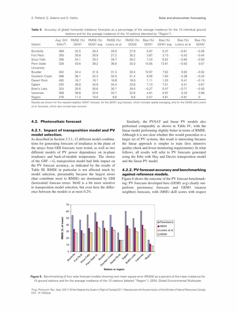
Table II. Accuracy of global horizontal irradiance forecasts as a percentage of the average irradiance for the 10 individual groundstations and for the average irradiance of the 10 stations (denoted by “Region”).

StationAvg. GHI(W/m2)

RMSE (%)GEM1

RMSE (%)GEM1 avg

RMSE (%)Lorenz et al.

RMSE (%)GEM2

Bias (%)GEM1

Bias (%)GEM1 avg

Bias (%)Lorenz et al.

Bias (%)GEM2

Bondville 369 32.5 28.4 29.0 27.9 5.97 5.37 �0.81 �0.26Fort Peck 350 30.8 26.8 27.2 26.2 3.87 3.13 �0.42 �0.44Sioux Falls 356 34.1 29.2 28.7 28.2 7.24 6.52 �0.60 �0.50Penn StateUniversity

326 43.6 38.2 36.8 35.0 14.05 13.81 �0.50 0.07

Boulder 402 34.4 31.8 31.3 30.4 10.97 7.62 0.62 �0.52Goodwin Creek 386 36.1 32.3 32.5 31.4 8.05 7.83 �0.38 �0.34Desert Rock 492 16.7 16.1 16.8 16.8 1.11 1.03 0.41 �0.14Egbert 325 38.8 34.8 34.4 33.6 7.13 7.51 0.41 0.67Bratt’s Lake 324 35.6 30.6 30.1 29.5 �0.27 0.47 �0.71 �0.40Varennes 308 39.8 32.6 33.7 32.6 4.81 0.97 0.43 0.58Region 476 11.4 10.0 8.8 8.8 5.57 4.81 �0.81 0

Results are shown for the nearest-neighbor GEM1 forecast, for the GEM1 avg forecast, which includes spatial averaging, and for the GEM2 and Lorenz

et al. forecasts, which also include bias removal.


4.2. Photovoltaic forecast

4.2.1. Impact of transposition model and PVmodel selection.As described in Section 3.3.1, 12 different model combina-tions for generating forecasts of irradiance in the plane ofthe arrays from GHI forecasts were tested, as well as twodifferent models of PV power dependence on in-planeirradiance and back-of-module temperature. The choiceof the GHI!Gi transposition model had little impact onthe PV forecast accuracy, as indicated by the results ofTable III. RMSE in particular is not affected much bymodel selection, presumably because the largest errors(that contribute most to RMSE) are dominated by GHI(horizontal) forecast errors. MAE is a bit more sensitiveto transposition model selection, but even here the differ-ence between the models is at most 0.2%.

Figure 5. Benchmarking of four solar forecast models showing root m10 ground stations and for the average irradiance of the 10 station


Similarly, the PVSAT and linear PV models alsoperformed comparably as shown in Table IV, with thelinear model performing slightly better in terms of RMSE.Although it is not clear whether this would generalize to alarger set of PV systems, this result is interesting becausethe linear approach is simpler to train (less intensivequality-check and fewer monitoring requirements). In whatfollows, all results will refer to PV forecasts generatedusing the Erbs with Hay and Davies transposition modeland the linear PV model.

4.2.2. PV forecast accuracyandbenchmarkingagainst reference models.Figure 6 shows the outcome of the PV forecast benchmark-ing: PV forecasts developed here (GEM1 avg) clearly out-perform persistence forecasts and GEM1 (nearestneighbor) forecasts, with (MSE) skill scores with respect

ean square error (RMSE) as a percent of the mean irradiance fos (labeled “Region”). GEM, Global Environmental Multiscale.

1. Reproducedwith the permission of theMinister ofNatural ResourcesCanada

r

.

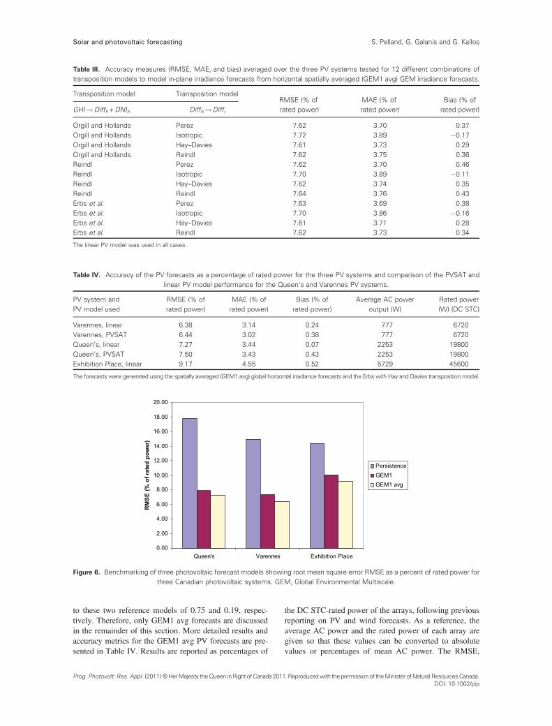
Table IV. Accuracy of the PV forecasts as a percentage of rated power for the three PV systems and comparison of the PVSAT andlinear PV model performance for the Queen’s and Varennes PV systems.

PV system andPV model used

RMSE (% ofrated power)

MAE (% ofrated power)

Bias (% ofrated power)

Average AC poweroutput (W)

Rated power(W) (DC STC)

Varennes, linear 6.38 3.14 0.24 777 6720Varennes, PVSAT 6.44 3.02 0.38 777 6720Queen’s, linear 7.27 3.44 0.07 2253 19800Queen’s, PVSAT 7.50 3.43 0.43 2253 19800Exhibition Place, linear 9.17 4.55 0.52 5729 45600

The forecasts were generated using the spatially averaged (GEM1 avg) global horizontal irradiance forecasts and the Erbs with Hay and Davies transposition model.

Figure 6. Benchmarking of three photovoltaic forecast models showing root mean square error RMSE as a percent of rated power forthree Canadian photovoltaic systems. GEM, Global Environmental Multiscale.

Table III. Accuracy measures (RMSE, MAE, and bias) averaged over the three PV systems tested for 12 different combinations oftransposition models to model in-plane irradiance forecasts from horizontal spatially averaged (GEM1 avg) GEM irradiance forecasts.

Transposition model Transposition modelRMSE (% ofrated power)

MAE (% ofrated power)

Bias (% ofrated power)GHI!Diffh+DNIh Diffh!Diffi

Orgill and Hollands Perez 7.62 3.70 0.37Orgill and Hollands Isotropic 7.72 3.89 �0.17Orgill and Hollands Hay–Davies 7.61 3.73 0.29Orgill and Hollands Reindl 7.62 3.75 0.36Reindl Perez 7.62 3.70 0.46Reindl Isotropic 7.70 3.89 �0.11Reindl Hay–Davies 7.62 3.74 0.35Reindl Reindl 7.64 3.76 0.43Erbs et al. Perez 7.63 3.69 0.38Erbs et al. Isotropic 7.70 3.86 �0.16Erbs et al. Hay–Davies 7.61 3.71 0.28Erbs et al. Reindl 7.62 3.73 0.34

The linear PV model was used in all cases.


to these two reference models of 0.75 and 0.19, respec-tively. Therefore, only GEM1 avg forecasts are discussedin the remainder of this section. More detailed results andaccuracy metrics for the GEM1 avg PV forecasts are pre-sented in Table IV. Results are reported as percentages of


the DC STC-rated power of the arrays, following previousreporting on PV and wind forecasts. As a reference, theaverage AC power and the rated power of each array aregiven so that these values can be converted to absolutevalues or percentages of mean AC power. The RMSE,



MAE, and bias as a percentage of rated power range from6.4% to 9.2%, 3.1% to 4.6%, and 0% to 0.5%, respec-tively. So that these numbers can be put into perspective,the average AC power output of these PV systems is ofthe order of 11% to 12% of the rated power. These accura-cies can be compared with those obtained by Lorenz et al.[2] for roughly 380 PV systems in two control areas ofGermany where they found day-ahead forecast RMSEs inthe range of 4% to 5% of rated power and biases of about1%. Given that error reduction occurs as the number ofstations and the geographical area over which they arespread increase, it is reasonable to expect comparableresults for Ontario when centralized PV forecasting isimplemented.

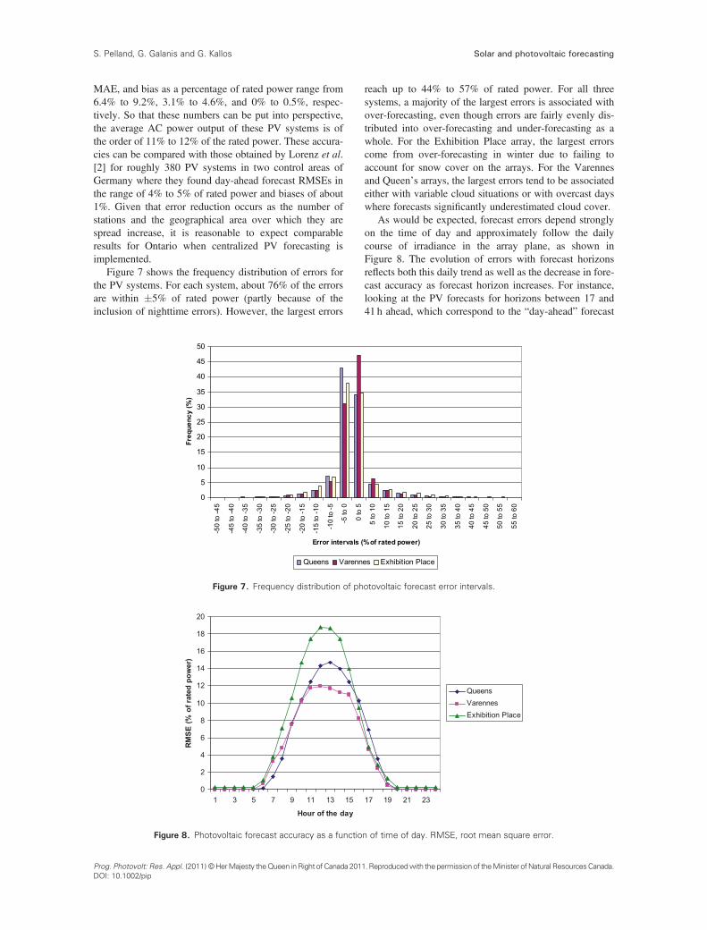
Figure 7 shows the frequency distribution of errors forthe PV systems. For each system, about 76% of the errorsare within �5% of rated power (partly because of theinclusion of nighttime errors). However, the largest errors

Figure 7. Frequency distribution of ph

Figure 8. Photovoltaic forecast accuracy as a functio


reach up to 44% to 57% of rated power. For all threesystems, a majority of the largest errors is associated withover-forecasting, even though errors are fairly evenly dis-tributed into over-forecasting and under-forecasting as awhole. For the Exhibition Place array, the largest errorscome from over-forecasting in winter due to failing toaccount for snow cover on the arrays. For the Varennesand Queen’s arrays, the largest errors tend to be associatedeither with variable cloud situations or with overcast dayswhere forecasts significantly underestimated cloud cover.

As would be expected, forecast errors depend stronglyon the time of day and approximately follow the dailycourse of irradiance in the array plane, as shown inFigure 8. The evolution of errors with forecast horizonsreflects both this daily trend as well as the decrease in fore-cast accuracy as forecast horizon increases. For instance,looking at the PV forecasts for horizons between 17 and41 h ahead, which correspond to the “day-ahead” forecast

otovoltaic forecast error intervals.

n of time of day. RMSE, root mean square error.

1. Reproducedwith the permission of theMinister ofNatural ResourcesCanada.

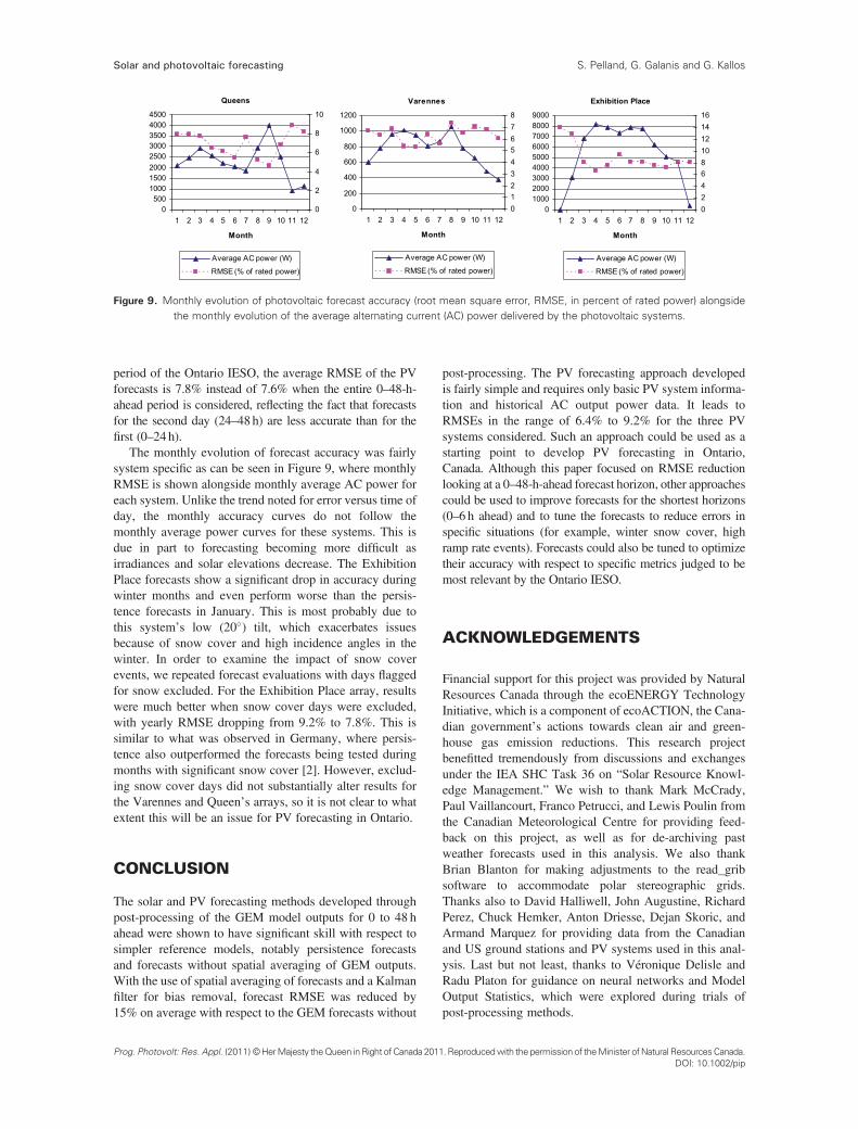
Figure 9. Monthly evolution of photovoltaic forecast accuracy (root mean square error, RMSE, in percent of rated power) alongsidethe monthly evolution of the average alternating current (AC) power delivered by the photovoltaic systems.


period of the Ontario IESO, the average RMSE of the PVforecasts is 7.8% instead of 7.6% when the entire 0–48-h-ahead period is considered, reflecting the fact that forecastsfor the second day (24–48h) are less accurate than for thefirst (0–24h).

The monthly evolution of forecast accuracy was fairlysystem specific as can be seen in Figure 9, where monthlyRMSE is shown alongside monthly average AC power foreach system. Unlike the trend noted for error versus time ofday, the monthly accuracy curves do not follow themonthly average power curves for these systems. This isdue in part to forecasting becoming more difficult asirradiances and solar elevations decrease. The ExhibitionPlace forecasts show a significant drop in accuracy duringwinter months and even perform worse than the persis-tence forecasts in January. This is most probably due tothis system’s low (20�) tilt, which exacerbates issuesbecause of snow cover and high incidence angles in thewinter. In order to examine the impact of snow coverevents, we repeated forecast evaluations with days flaggedfor snow excluded. For the Exhibition Place array, resultswere much better when snow cover days were excluded,with yearly RMSE dropping from 9.2% to 7.8%. This issimilar to what was observed in Germany, where persis-tence also outperformed the forecasts being tested duringmonths with significant snow cover [2]. However, exclud-ing snow cover days did not substantially alter results forthe Varennes and Queen’s arrays, so it is not clear to whatextent this will be an issue for PV forecasting in Ontario.

CONCLUSION

The solar and PV forecasting methods developed throughpost-processing of the GEM model outputs for 0 to 48 hahead were shown to have significant skill with respect tosimpler reference models, notably persistence forecastsand forecasts without spatial averaging of GEM outputs.With the use of spatial averaging of forecasts and a Kalmanfilter for bias removal, forecast RMSE was reduced by15% on average with respect to the GEM forecasts without


post-processing. The PV forecasting approach developedis fairly simple and requires only basic PV system informa-tion and historical AC output power data. It leads toRMSEs in the range of 6.4% to 9.2% for the three PVsystems considered. Such an approach could be used as astarting point to develop PV forecasting in Ontario,Canada. Although this paper focused on RMSE reductionlooking at a 0–48-h-ahead forecast horizon, other approachescould be used to improve forecasts for the shortest horizons(0–6 h ahead) and to tune the forecasts to reduce errors inspecific situations (for example, winter snow cover, highramp rate events). Forecasts could also be tuned to optimizetheir accuracy with respect to specific metrics judged to bemost relevant by the Ontario IESO.

ACKNOWLEDGEMENTS

Financial support for this project was provided by NaturalResources Canada through the ecoENERGY TechnologyInitiative, which is a component of ecoACTION, the Cana-dian government’s actions towards clean air and green-house gas emission reductions. This research projectbenefitted tremendously from discussions and exchangesunder the IEA SHC Task 36 on “Solar Resource Knowl-edge Management.” We wish to thank Mark McCrady,Paul Vaillancourt, Franco Petrucci, and Lewis Poulin fromthe Canadian Meteorological Centre for providing feed-back on this project, as well as for de-archiving pastweather forecasts used in this analysis. We also thankBrian Blanton for making adjustments to the read_gribsoftware to accommodate polar stereographic grids.Thanks also to David Halliwell, John Augustine, RichardPerez, Chuck Hemker, Anton Driesse, Dejan Skoric, andArmand Marquez for providing data from the Canadianand US ground stations and PV systems used in this anal-ysis. Last but not least, thanks to Véronique Delisle andRadu Platon for guidance on neural networks and ModelOutput Statistics, which were explored during trials ofpost-processing methods.



REFERENCES

1. Ontario Power Authority Feed-In Tariff website, http://fit.powerauthority.on.ca/ (February 23, 2011).

2. Lorenz E, Scheidsteger T, Hurka J, Heinemann D,Kurz C. Regional PV power prediction for improvedgrid integration. Progress in Photovoltaics: Researchand Applications 2010; n/a doi: 10.1002/pip.1033.

3. Lorenz E, Hurka J, Heinemann D, Beyer HG. Irradianceforecasting for the power prediction of grid-connectedphotovoltaic systems. IEEE Journal of Selected Topicsin Applied Earth Observations and Remote Sensing2009; 2(1): 2–10, doi: 10.1109/JSTARS.2009.2020300.

4. Focken U, Lange M, Mönnich K, Waldl HP, BeyerHG, Luig A. Short-term prediction of the aggregatedpower output of wind farms—a statistical analysis ofthe reduction of the prediction error by spatialsmoothing effects. Journal of Wind Engineeringand Industrial Aerodynamics 2002; 90: 231–246.

5. Lorenz E, Remund J, Müller SC, et al. Benchmarkingof different approaches to forecast solar irradiance. Pro-ceedings of the 24th European Photovoltaic Solar EnergyConference 2009; Hamburg, Germany: pp. 4199–4208,doi: 10.4229/24thEUPVSEC2009-5BV.2.50.

6. Mailhot J, Bélair S, Lefaivre L, et al. The 15-kmversion of the Canadian regional forecast system.Atmosphere-Ocean 2006; 44: 133–149.

7. Environment Canada weather office website, http://www.weatheroffice.gc.ca/grib/index_e.html, (February 23,2011).

8. Read_grib open source program, http://workhorse.europa.renci.org/~bblanton/ReadGrib/, (February 23, 2011).

9. World Meteorological Organization. Guide to meteo-rological instruments and methods of observation.WMO-No. 8 (Seventh edition), 2008. Available onlineat: http://www.wmo.int/pages/prog/www/IMOP/publica-tions/CIMO-Guide/CIMO_Guide-7th_Edition-2008.html

10. National Oceanic and Atmospheric Administration-website, SURFRAD (Surface Radiation) Networkhttp://www.srrb.noaa.gov/surfrad/, (February 23, 2011).

11. Hoyer-Klick C, Beyer HG, Dumortier D, et al. Man-agement and exploitation of solar resource knowledge.Proceedings of Eurosun 2008; Lisbon, Portugal.

12. Environment Canada National Climate Data and In-formation Archive, http://climate.weatheroffice.gc.ca/climateData/canada_e.html, (February 23, 2011).

13. Beyer HG, Polo Martinez J, Suri M, et al. D 1.1.3 Re-port on Benchmarking of Radiation Products. Report


under contract no. 038665 of MESoR, available fordownload at http://www.mesor.net/deliverables.html,(February 23, 2011).

14. Louka P, Galanis G, Siebert N, et al. Improvements inwind speed forecasts for wind power predictionpurposes using Kalman filtering. Journal of WindEngineering and Industrial Aerodynamics 2008; 96:2348–2362.

15. Galanis G, Louka P, Katsafados P, Kallos G, PytharoulisI. Applications of Kalman filters based on non-linearfunctions to numerical weather predictions. Annals ofGeophysics. 2006; 24: 2451–2460.

16. Rigollier C, Bauer O, Wald L. On the clear sky modelof the ESRA—European Solar Radiation Atlas—withrespect to the Heliosat method. Solar Energy 2000;68(1): 33–48.

17. Orgill JF, Hollands KGT. Correlation equation forhourly diffuse radiation on a horizontal surface. SolarEnergy 1977; 19(4): 357–359.

18. Erbs DG, Klein SA, Duffie JA. Estimation of thediffuse radiation fraction for hourly, daily andmonthly-average global radiation. Solar Energy1982; 28(4): 293–302.

19. Reindl DT, Beckman WA, Duffie JA. Diffuse fractioncorrelations. Solar Energy 1990; 45(1): 1–7.

20. Perez R, Ineichen P, Seals R, Michalsky J, Stewart R.Modeling daylight availability and irradiance compo-nents from direct and global irradiance. Solar Energy1990; 44(5): 271–289, doi: 10.1016/0038-092X(90)90055-H.

21. Duffie JA, Beckman WA. Solar Engineering ofThermal Processes. Wiley: New York, 1991; 94–95.

22. Hay JE, Davies JA, Calculation of the solar radiationincident on an inclined surface, Proceedings FirstCanadian Solar Radiation Workshop 1980: 59–72.

23. Reindl DT, Beckman WA, Duffie JA. Evaluation ofhourly tilted surface radiation models. Solar Energy1990; 45(1): 9–17.

24. Drews A, de Keizer AC, Beyer HG, et al. Monitoringand remote failure detection of grid-connected PVsystems based on satellite observations. Solar Energy2007; 81(4): 548–564, doi:10.1016/j.solener.2006.06.019.

25. Perez R, Beauharnois M, Hemker K, et al. Evaluationof numerical weather prediction solar irradianceforecasts in the US. In preparation (to be presented atthe 2011 ASES Annual Conference).


http://fit.powerauthority.on.ca/

http://fit.powerauthority.on.ca/

http://www.weatheroffice.gc.ca/grib/index_e.html

http://www.weatheroffice.gc.ca/grib/index_e.html

http://workhorse.europa.renci.org/~bblanton/ReadGrib/

http://workhorse.europa.renci.org/~bblanton/ReadGrib/

http://www.wmo.int/pages/prog/www/IMOP/publications/CIMO-Guide/CIMO_Guide-7th_Edition-2008.html

http://www.wmo.int/pages/prog/www/IMOP/publications/CIMO-Guide/CIMO_Guide-7th_Edition-2008.html

http://climate.weatheroffice.gc.ca/climateData/canada_e.html



http://www.mesor.net/deliverables.html

solar and photovoltaic forecasting through post...

Documents