lable at ScienceDirect

Renewable Energy 91 (2016) 11e20

Contents lists avai

Renewable Energy

journal homepage: www.elsevier .com/locate/renene

Day-ahead forecasting of solar power output from photovoltaic plantsin the American Southwest

David P. Larson, Lukas Nonnenmacher, Carlos F.M. Coimbra*

Department of Mechanical and Aerospace Engineering, Jacobs School of Engineering, Center of Excellence in Renewable Energy Integration and Center forEnergy Research, University of California San Diego, La Jolla, CA 92093, USA

a r t i c l e i n f o

Article history:Received 2 July 2015Received in revised form30 November 2015Accepted 8 January 2016Available online xxx

Keywords:ForecastingSolar power outputPhotovoltaicsNumerical weather predictionInterannual performance variability

* Corresponding author.E-mail address: ccoimbra@ucsd.edu (C.F.M. Coimb

http://dx.doi.org/10.1016/j.renene.2016.01.0390960-1481/© 2016 Elsevier Ltd. All rights reserved.

a b s t r a c t

A forecasting method for hourly-averaged, day-ahead power output (PO) from photovoltaic (PV) powerplants based on least-squares optimization of Numerical Weather Prediction (NWP) is presented. Threevariations of the forecasting method are evaluated against PO data from two non-tracking, 1 MWp PVplants in California for 2011e2014. The method performance, including the inter-annual performancevariability and the spatial smoothing of pairing the two plants, is evaluated in terms of standard errormetrics, as well as in terms of the occurrence of severe forecasting error events. Results validate theperformance of the proposed methodology as compared with previous studies. We also show that thebias errors in the irradiance inputs only have a limited impact on the PO forecast performance, since themethod corrects for systematic errors in the irradiance forecast. The relative root mean square error(RMSE) for PO is in the range of 10.3%e14.0% of the nameplate capacity, and the forecast skill ranges from13% to 23% over a persistence model. Over three years, an over-prediction of the daily PO exceeding 40%only occurs twice at one of the two plants under study, while the spatially averaged PO of the pairedplants never exceeds this threshold.

© 2016 Elsevier Ltd. All rights reserved.

1. Introduction

High renewable energy penetration grids are challenging tobalance due to inherently variable generation weather-dependentenergy resources. Solar and wind forecasting are proven methodsfor mitigating resource uncertainty and reducing the need forscheduling of ancillary generation. Several forecasting methodol-ogies have been developed to target different forecast time hori-zons [1].

Short-term forecasting (t < 1 h) is mainly based on sky imagingtechniques and time-series models, while satellite-based forecastsachieve usable results for time horizons of 1e6 h [2e4]. Usually,horizons larger than 6 h require numerical weather predictionmodels (NWP) to generate accurate results, although there areexceptions such as [5]. Recent advances in solar forecasting havemainly covered intra-day resource forecasts, driven by advances insky image techniques and time-series modeling [6e16].

While intra-day forecasts are important for grid stability, day-ahead forecasts are critical for market participation and unit

ra).

commitment. Current market regulations in many world regionsrequire day-ahead forecasts [17e19] and there are financial in-centives to produce accurate forecasts [18]. Besides market partic-ipation, day-ahead forecasts can also be useful for energy storagedispatch [20,21]. In this paper, we focus on day-ahead forecasting ofpower output from photovoltaic power plants in the AmericanSouthwest.

1.1. Previous work

Most NWP models generate global horizontal irradiance (GHI)at the ground level as one of the outputs, with some newer gen-eration models now including direct normal irradiance (DNI).Previous studies evaluated the accuracy of this GHI variable andsuggestedways to improve it, which havemostly focused on spatialaveraging and bias removal [22e28]. [22,27,29] showed that fore-cast errors for all sky conditions can be reduced by averaging theGHI forecasts from all NWP grid points within a set distance of thetarget site. In addition [22], showed that the forecast performancecould be further improved through bias removal using a poly-nomial regression based on the solar zenith angle and clear skyindex. [27] showed that a similar improvement can be achieved

D.P. Larson et al. / Renewable Energy 91 (2016) 11e2012

through Kalman filtering.In contrast to our knowledge of the performance of day-ahead

GHI predictions, the application of these forecasts directly to pre-diction of day-ahead power output (PO) of PV plants is poorly un-derstood. There are currently less than a dozen published studiesthat cover the subject of day-ahead PV PO forecasts, the majority ofwhich were published in the last 5 years. We summarize thesepapers below and in Table 1. It is important to note that this lack ofknowledge is partly due to the difficulty of obtaining data fromoperational PV plants, due to security restrictions and lack of datainfrastructure. However, data access should improve in the comingyears due to energy policies that require PO forecasting andtherefore necessitate the collection of PO data.

[30] applied the Danish Meteorological Institute's High Resolu-tion Limited Area Model (HIRLAM) to forecast PO of 21 PV systemsin Denmark. The PV systems had a total rated power capacity of1e4 kWp each and one year of data was used to evaluate theforecasts. HIRLAM GHI forecasts were used as the main input toautoregressive-based PO models. [31] also used HIRLAM to forecastPO of a 6.2 kWp test site in Spain.

[29] and [32] used the European Center for Medium-RangeWeather Forecasts Model (ECMWF) to generate regional, PO fore-casts in Germany. [29] only evaluated two months (April and July2006) of forecasts for 11 PV systems in Southern Germany, while[32] tested on 10 months (July 2009eApril 2010) of PO data fromapproximately 400 representative PV systems.

[33] used an artificial neural network (ANN) to predict GHI inTrieste, Italy. The predicted GHI was then mapped directly to POusing the efficiency data of the studied 20 kWp PV system. Unfor-tunately, PO forecast results were only reported for four consecu-tive clear sky days in May 2009. Similarly [34], evaluated anautoregressive-moving-average model with exogenous inputs(ARMAX) forecast model that did not use NWP data as input.However [34], only forecasted the day-ahead mean daily PO, ratherthan day-ahead hourly values, for a 2.1 kWp PV system in China.

[27] forecasted PO of three small PV systems (6.72, 19.8 and45.6 kWp) in mainland Canada, using the Canadian MeteorologicalCentre's Global Environmental Multiscale Model (GEM). The GEM'sGHI forecasts were validated against ground measurements fromthe SURFRAD Network in the United States. Spatial averaging of300 kme600 km and bias removal via Kalman filtering were usedto improve the GEM forecast performance. Reported RMSE valueswere in the range of 6.4%e9.2% of the rated power of the PV sys-tems for a 1 year testing set (April 2008eMarch 2009).

[35] and [36] generated regional forecasts for Japan using Sup-port Vector Regression (SVR) together with inputs from theJapan Meteorological Agency's Grid Point Value-Mesoscale Model

Table 1Summary of the current literature on day-ahead PO forecasting. “Type” refers towhether thow much data was used in the forecast model evaluation.

Region NWP model Type

[30] Denmark HIRLAM Point[31] Spain HIRLAM Point[29] Germany ECMWF Regional[32] Germany ECMWF Regional[35] Japan GPV-MSM Regional[36] Japan GPV-MSM Regional[27] Canada GEM Point[37] France ARPEGE Point[38] France ARPEGE Point[39] Spain WRF Point[33] Italy N/A Point[34] China N/A Point

(GPV-MSM). [35] used PO data from approximately 450 PV plantsfrom four regions (Kanto, Chubu, Kansai, Kyushu) that had a netrated power of approximately 15 MWp while [36] used data from273 PV plants spread over two regions (Kanto and Chubu), with anapproximate total power of 8 MWp.

[37] and [38] forecasted PO of 28 PV plants in mainland Franceusing Meteo France's Action de Recherche Petite Echelle GrandeEchelle (ARPEGE) model. [37] presented a deterministic forecastthat achieved a RMSE of 8e12% of the plant capacity over two yearsof testing data (2009e2010) while [38] presented a probabilisticforecast. Both methods used 31 variables from the ARPEGE,including GHI as well as environmental conditions, e.g., tempera-ture, humidity and precipitation. Unfortunately, no actual valueswere reported for the PV plant power ratings or other technicaldetails, which limits analysis into the applicability of the results toother PV plants and regions.

Most recently [39], forecasted the PO of five vertical-axistracking PV plants in Spain, using a nonparametric model basedon the Weather Research and Forecasting Model (WRF). The PVplants ranged in size from 775 to 2000 kWp and the forecasts wereevaluated with data from 2009 to 2010. Quantile Regression For-ests, a variation of random forests, was used to generate the POforecasts, with WRF variables such as GHI, temperature and cloudcover as the inputs.

Although these studies all presented day-ahead PO forecastingfor PV plants, further research is still required, especially for sites inthe United States. In this study we seek to provide the followingcontributions: (1) Introduction and evaluation of a PV PO forecastmodel for the American Southwest, a region with both high solarenergy generation potential and a favorable political environmentfor solar, especially in California. (2) Investigation of the interan-nual forecast performance variability and (3) the occurrence ofsevere forecasting errors, as they relate to large-scale renewableenergy integration. (4) Spatial smoothing through pairing of PVplants in proximity. To achieve these goals, we systematically testapproaches and inputs to generate PO forecasts based on twooperational PV plants in Southern California.

2. Data

2.1. Ground data

Two sites are used to evaluate day-ahead forecasts of GHI andPO: Canyon Crest Academy (CCA) and La Costa Canyon High School(LCC). CCA (32.959�, �117.190�) and LCC (33.074�, �117.230�) areboth located in San Diego County, USA, and each feature 1MWpeak(MWp) of non-tracking photovoltaic (PV) panels. The PV panels for

he forecast was for a single PV plant site or for an entire regionwhile “Testing data” is

PV plants

No. of sites Total capacity Testing data

21 ~100 kWp 1 year1 6 kWp 10 months

11 Unknown 2 months383 ~100 MWp 10 months454 ~10 MWp 1 year273 ~10 MWp 1 year

3 ~100 kWp 2 years28 Unknown 2 years28 Unknown 2 years5 ~10 MWp 2 years1 20 kWp 4 days1 2 kWp 6 months

D.P. Larson et al. / Renewable Energy 91 (2016) 11e20 13

both sites were installed in 2011 as part of a power purchaseagreement (PPA) between the San Dieguito Union High SchoolDistrict and Chevron Energy Solutions.

Each site has two inverters, with the PV panels mounted abovethe parking lots at a 5� incline. At CCA, the panels are split over twoparking lots, approximately 200 m apart and each with 500 kWp.Due to the site's characteristics, the north parking lot panels face(~20�) southwest, while the south parking lot panels face directlysouth. Meanwhile, the panels at LCC cover a single parking lot andface ~30� southwest.

Total PO from the PV panels at each site is available as 15-minaverages. Additionally, 15-min averaged GHI data is available fromco-located pyranometers. Fig. 1 illustrates the data availability forboth sites. For this study, the GHI and PO data are backwards-averaged to hourly values and night values are removed, wherewe define night as zenith angles (qz) greater than 85�. Note that themaximum observed PO of CCA matches the nameplate capacity(1 MWp), while the maximum observed PO of LCC peaks atz0.8 MW, despite both sites using identical PV technologies. Thisdifference is due to the greater (~30�) southwest orientation of thePV panels at LCC.

2.2. NWP data

We use forecasted variables from two publicly-available NWPmodels: the North AmericanMesoscale Forecast System (NAM) andthe Regional Deterministic Prediction System (RDPS).

2.2.1. NAMThe NAM is a NWPmodel provided by the National Oceanic and

Atmospheric Administration (NOAA) on a z12 km � 12 km spatialgrid that covers the continental United States. Forecasts aregenerated four times daily at 00Z, 06Z, 12Z and 18Z, with hourlytemporal resolution for 1e36 h horizons and 3 h resolution for39e84 h horizons. Downward shortwave radiative flux (DSWRF)[W/m2] at the surface, a synonym for GHI, is forecasted using theGeophysical Fluid Dynamics Laboratory Shortwave radiativetransfer model (GFDL-SW) [40]. The NAM also forecasts total cloudcover (TCDC) [%], where the entire atmosphere is treated as a singlelayer.

In this study, NAM forecasts generated at 00Z were downloadedfrom the NOAA servers and degribbed for September 2013 toNovember 2014, for all nodes within 200 km of CCA and LCC. Fig. 2shows the distribution of NAM forecast nodes over SouthernCalifornia.

Fig. 1. Availability of ground measurements of GHI and PO for CCA (left column) and LCC (r

2.2.2. RDPSThe Canadian Meteorological Centre generates the RDPS model

on a 10 km � 10 km spatial grid covering North America. As withthe NAM, RDPS forecasts total cloud cover (TCDC) as a percentagefor each grid element, not distinguishing between the layers of theatmosphere. The operational RDPS model generates forecasts dailyat 00Z, 06Z, 12Z and 18Z with hourly temporal resolution. Only the00Z forecasts are used in this study, to ensure fair comparison withthe NAM forecasts. RDPS GHI forecasts were not available.

3. Forecasting models

3.1. Persistence

We include a day-ahead persistence forecast of both GHI and POas a baseline. The persistence forecast assumes that the currentconditions will repeat for the specified time horizon. In otherwords:

bytþt ¼ yt ; (1)

where bytþt is the forecasted value of some variable y, at a timehorizon of t from some initial time t. For day-ahead persistence,t ¼ 24 h.

3.2. Deterministic cloud cover to GHI model

We use a modified version of the deterministic model fromRefs. [19,41,42] to derive GHI from cloud cover:

GHI ¼ GHICS½0:35þ 0:65ð1� CCÞ�; (2)

where CC is the TCDC (0¼ clear, 1¼ overcast) from the NWPmodeland GHICS is the clear sky GHI from the airmass independent modeldescribed in Refs. [43e45].

3.3. Effects of spatial averaging

Previous studies have shown that NAMGHI forecast error can bereduced by spatially averaging the forecasts from all nodes within aset distance of the target site [22,27]. The distance (d) in km be-tween a site and a NAM node can be calculated using the sphericallaw of cosines:

d ¼ arccos½sinðf1Þsinðf2Þ þ cosðf1Þcosðf2Þcosðl2 � l1Þ�R; (3)

where (øi, li) is the latitudeelongitude for a point i and R is the

ight column). The missing GHI data from LCC is due to a malfunctioning pyranometer.

Fig. 2. Map of Southern California, with the NAM grid points marked with gray dots. UC San Diego (UCSD; star), Canyon Crest Academy (CCA; triangle) and La Costa Canyon (LCC;square) are also marked on the map. The area to the lower left is the Pacific Ocean, with Mexico shown in the bottom right.

D.P. Larson et al. / Renewable Energy 91 (2016) 11e2014

radius of the Earth (6371 km). For both CCA and LCC, there areapproximately 50 NAM nodes with 50 km, 200 nodes within100 km, and 800 nodes within 200 km.

Fig. 3 shows the effect spatial averaging of the NAMGHI GHIforecasts for CCA compared to using only the NAM node closest tothe site, i.e., the naive node choice. The NAM forecasts from theavailable data set (September 2013eNovember 2014) are groupedinto bins based on the clear sky index (kt),

Fig. 3. Effect of spatial averaging the NAMGHI GHI forecasts for CCA September2013eNovember 2014. Naive refers to the NAM node physically closest to the site,while 50 km, 100 km, and 200 km are the unweighted average forecasts of all nodeswithin each search radius. Each marker represents the average RMSE of all forecastsgenerated for each kt bin, i.e., each group of sky conditions.

kt ¼ GHIGHICS

; (4)

which provides a measure of the sky conditions during the fore-casted time period (kt / 0: overcast, kt / �>1: clear). Then, theroot mean square error (RMSE) is calculated between the forecastsin each kt bin and the ground truth, and averaged to produce oneRMSE value per kt bin. The result is that spatial averaging reducesthe RMSE of the forecasts for all sky conditions, as compared to thenaive node choice. This is consistent with results presented inprevious work, e.g. Refs. [22,27].

Hereafter, we will report results for the naive NAM forecasts(NAMGHI, NAMCC) as well as the 100 km spatially averaged versions(NAM*

GHI, NAM*CC). 100 km is chosen over 200 km as there is a

negligible difference in error between the two. Also, the 100 kmcase requires approximately 25% the NAM grid points as the200 km case, and therefore has lower storage and computationalrequirements.

3.4. GHI to PO model

As the PV panels at both sites are non-tracking, we assume thatthere exists a linear function f($) that can map GHI to PO. Fig. 4illustrates the relationship between GHI and PO for CCA over afull year (September 2013eNovember 2014), with a referencelinear fit included (R2 ¼ 0.97). The high R2 value (>0.95) indicatesthat a linear mapping between GHI and PO is not an unreasonableassumption.

Formally, we define a linear function f(x;w) as:

f ðx;wÞ ¼Xnj¼0

wjxj ¼ wTx; (5)

Fig. 4. GHI vs. PO for CCA over September 2013eNovember 2014, ignoring night values(qz > 85�). Each marker is a single data point, and the line is a least-squares fit betweenGHI and PO with a R2 value of 0.97.

Table 2Day-ahead GHI forecast performance for CCA, from September 2013 to November2014. Night values have been removed (night ≡ qz � 85�). No post-processing ormodel output statistics (MOS) have been applied to the forecasts. The errors arerelative to the mean GHI of the considered period (515 Wm�2). Bold values indicatebest performances.

Method MAE [%] MBE [%] RMSE [%] s [e]

Persistence 24.9 7.7 36.2 e

RDPSCC 20.3 2.3 27.5 0.24NAMGHI 21.9 �11.6 31.8 0.12

NAM*GHI

20.5 �7.6 28.3 0.22

NAMCC 26.4 14.1 35.3 0.03

NAM*CC

26.2 16.2 32.7 0.10

D.P. Larson et al. / Renewable Energy 91 (2016) 11e20 15

where w is the weight vector, x is the input vector, x0 ¼ 1 byconvention, and n is the number of model parameters. Thenwe useordinary least-squares to find the optimal weights w*, i.e., theweights that minimize the error between the predictor f(x;w) andthe true value y.

More specifically, for a given set of m example inputs {x(1), …,x(m)} and outputs {y(1), …, y(m)}, the least-squares costs function isdefined as:

JðwÞ ¼Xmi¼1

�f�xðiÞ;w

�� yðiÞ

�2 ¼ kXw� yk22: (6)

The optimal weights w* are then the w that minimizes the costfunction:

w� ¼ minw

kXw� yk22; (7)

where X2ℝm�n, w2ℝn, and y2ℝm.For the purposes of this study, we use the predicted GHI (dGHI)

from one of the NWP models and zenith angle (qZ) as the modelinputs. I.e. n ¼ 2, x1 ¼ dGHI and x2 ¼ qz, where qz is included so thattemporal information is encoded into the model. Readers arereferred to [46] and [47] for more detailed studies into modeling ofPO of PV power plants.

4. Results and discussion

4.1. Error metrics

We use standard error metrics to evaluate the performance ofboth the GHI and PO forecasts: Mean Absolute Error (MAE), MeanBias Error (MBE), Root Mean Square Error (RMSE), and skill (s) [7]:

MAE ¼ 1N

XNi¼1

jeij; (8)

MBE ¼ 1N

XNi¼1

ei; (9)

RMSE ¼ffiffiffiffiffiffiffiffiffiffiffiffiffiffiffiffiffiffi1N

XNi¼1

e2i

vuut ; (10)

s ¼ 1� RMSERMSEp

; (11)

where N is the number of forecasts, RMSEp is the RMSE of thepersistence forecast, and e is the error between the true value (y)and forecasted value (by):ei ¼ yi � byi: (12)

Additionally, for ease of comparison to previously publishedresults, we also include normalized RMSE (nRMSE):

nRMSE ¼ffiffiffiffiffiffiffiffiffiffiffiffiffiffiffiffiffiffiffiffiffiffiffiffiffiffi1N

XNi¼1

�eiy

�2vuut ; (13)

where y is the mean true value over the considered period, e.g.,September 2013eNovember 2014.

4.2. GHI forecast performance

Day-ahead GHI forecast performance and statistics for CCA forSeptember 2013eNovember 2014 are shown in Table 2. As noted inSection 3.3, the spatially averaged forecasts (NAM*

GHI and NAM*CC)

use all NAM nodes within 100 km of the site. The best GHI forecastis generated with RPDS, which reduces the RMSE 24% as comparedto the persistence model. NAMCC performs the worst, reducingRMSE only by 3% compared to persistence. However, the resultspresented are for GHI forecasts that have not undergone any post-processing or model output statistics (MOS), which have beenshown to improve forecast performance (see Refs. [22,25]).

Without post-processing or MOS, the GHI forecasts underper-form as compared to prior literature. Two of the most extensivestudies on day-ahead GHI forecasting are [27] and [26]. In Ref. [27],the GEM NWP model is evaluated using seven SURFRAD Networksites in the US and achieves RMSE values in the range ofz80e120 Wm�2 [26]. expands on [27] by providing results for avariety of common NWPmodels, including GEM, ECMWF andWRF.RMSE values reported in Ref. [26] are in the range of 70e200,90e130, 80e115, and 95e135 Wm�2 for sites in the US, CentralEurope, Spain and Canada respectively. Unfortunately, neitherstudy directly evaluated RDPS or NAM.

4.3. Power output forecast performance

PO is forecasted for both CCA and LCC using the methodsdescribed in Section 3. For the 18 months of overlapping data

D.P. Larson et al. / Renewable Energy 91 (2016) 11e2016

between the ground measurements and NWP models, odd monthsare used for the training set and even months for the testing set.Splitting the sets in this way, rather than in sequential partitions,ensures that the models are trained on data from all four seasons.Besides this monthly training, the effects of training on a full year ofdata and testing on another full year are discussed in Section 4.4.

Fig. 5 shows three exemplary days of forecasted and measuredPO. The persistence model performs well on the first (clear) day,with no visible difference to the measured PO, while both NWP-based forecasts under-predict the PO. On the second exemplaryday, the NWP-based models perform better than on the first day,but do not beat the persistence model. Since the persistence modelis just a repetition of the previous day, persistence works well if theweather conditions between days do not change. Hence, persis-tence also outperforms the NWPmodels because it inherits a betterrepresentation of the temperature effects on the panels that are notan input to the GHI to POmodel. However, the strength of the NWPmodels is to predict cloud cover and irradiance attenuation, and arehence performing better when conditions change between days.The third exemplary day shows this effect, where the persistencemodel under-predicts since the previous day (not shown) wasovercast. These results are expected and consistent with previousfindings on the performance of the persistence model [3,24].

Table 3 summarizes the PO forecast results and shows that allthree NWP-based forecast models perform comparably for bothsites (s ¼ 19�25%) and overall outperform the persistence model.However, the persistencemodel has a lower absolute error than theNWP-basedmodels for 47% and 49% of the data points in the testingset for CCA and LCC respectively. This is likely a result of thetemperate climate at both sites, i.e., that both sites have an abun-dance of periods where the weather conditions do not change andtherefore the persistence model will excel.

Given the significant variations in skill for the GHI forecasts(s ¼ 10�24%), it might be surprising that all three PO forecastsperform almost equally well. However, the training of the GHI to POmodel removes biases in the forecasts. This seems to be anadvantage of our proposed model compared to [27], where theaccuracy of the PV output prediction was strongly impacted by theaccuracy of the GHI input.

4.4. Interannual performance variability

While all previous work has only focused on bulk error statistics,we also investigate the interannual performance variability. This isimportant since meteorological studies have shown that there are

Fig. 5. Sample days where the NWP-based forecasts (RDPSCC and NAM*GHI) for CCA pe

relatively strong interannual variations in many weather phe-nomenon, e.g., DNI [48]. However, this variation is unknown for theevaluation of PV PO. Quantifying this variation will enable us todefinewhat is a sufficient length of training and testing data sets forPO forecasts.

We compare the PO forecast performance per year for2011e2014. RDPSCC is used as the input source for the GHI to POmodel and themodel parameters are trained in the sameway as theprevious section. We use RDPSCC rather than NAMGHI and NAMCCfor two reasons. First, we have RDPSCC forecasts for the entirety of2011e2014, but NAM forecasts only for September2013eNovember 2014. Second, as discussed in the previous sec-tion, the PO forecast performance is not strongly influenced by theinput GHI forecast. Hence, we assume that the interannual RDPSCCforecast results in this section are representative of all evaluatedNWP-based models.

Table 4 shows the interannual performance variability of POforecasts for CCA and LCC over 2011e2014. The PO model is trainedseparately on 2011, 2012, and 2013, and then tested on the subse-quent years of data. For both CCA and LCC, the forecast performanceon the test set depends more on the test set itself rather than thetraining set used. For example, the CCA forecast models trained on2011, 2012 and 2013 achieved nRMSE values of 0.26, 0.30 and 0.28respectively on the training set. But all three models achievednRMSE of 0.24 on the 2014 testing set. A similar trend is seen in the2013 testing sets and the LCC forecasts.

Although there is no prior literature that reports day-ahead POforecast performance in our studied region of the AmericanSouthwest, it is important to consider our results in the context ofother work. As noted in Table 4, our forecast methodology achievesnRMSE values in the range of 0.24e0.33. [30,36,39] reportednRMSE values in the range of 0.08e0.13, 0.26e0.35, and 0.10e0.30respectively. Each study used at least 1 year of testing data, but the21 PV systems in Ref. [30] had nameplate capacities of only1e4 kWp. [36] and [39] evaluated forecasts with PV systems of totalcapacity ~10 MWp, and achieved nRMSE values closer in range toour results.

Error distributions are another important factor in evaluatingforecast performance. Fig. 6 shows the forecast error distributionsof three trainingetesting data sets and three sites: CCA, LCC and athird fictional site denoted as “Combined”. The “Combined” siteallows us to consider the impact of pairing the two PV plants tosimulate a single, spatially distributed 2 MWp power plant. Allthree sites and trainingetesting sets show similar distributions,with peaks centered at less than zero error. 2012 and 2013 have a

rform (a) worse than; (b) as good as; and (c) better than day-ahead persistence.

Table 3Day-ahead hourly PO forecasts for CCA and LCC, with MAE, MBE and RMSE reported as relative to the rated plant capacity of each site (1 MWp). The models were trained andtested using hourly data from September 2013eNovember 2014, with odd months used for training and even months for testing.

Site Method Training Testing

MAE [%] MBE [%] RMSE [%] s [e] MAE [%] MBE [%] RMSE [%] s [e]

CCA Persistent 9.0 0.4 15.6 e 8.8 �0.5 14.7 e

RDPSCC 8.9 0.0 12.5 0.20 8.4 0.2 11.5 0.21NAMGHI 9.6 �0.0 13.2 0.15 8.5 �0.3 11.3 0.23

NAM*GHI

9.3 0.0 12.7 0.18 8.4 �0.2 11.0 0.25

NAMCC 9.2 �0.0 12.8 0.18 8.8 0.1 11.6 0.21

NAM*CC

9.1 �0.0 12.5 0.20 8.5 0.4 11.2 0.23

LCC Persistent 8.0 0.3 14.0 e 7.2 �0.3 12.0 e

RDPSCC 7.7 0.0 11.1 0.21 7.3 0.6 9.8 0.19NAMGHI 8.1 0.0 11.6 0.17 7.3 0.2 9.5 0.21

NAM*GHI

8.0 0.0 11.2 0.20 7.2 0.3 9.3 0.23

NAMCC 8.1 0.0 11.4 0.18 7.7 0.4 9.8 0.18

NAM*CC

8.0 0.0 11.2 0.20 7.3 0.6 9.5 0.21

Table 4Interannual variability of NWP-based PO forecasts for CCA and LCC. RDPSCC is used as the NWP input for the forecast, with night values removed (night ≡ qz > 85�). The GHI-to-PO model is trained on one year of data and then tested on a separate year. RMSE is reported as relative to the PV plant capacity (1 MWp for CCA and LCC) while nRMSE iscalculated using Equation (13) and the mean PO (PO) of the considered period. Higher forecast skills (s) indicate better performance.

Training Testing

Year PO [kW] RMSE [%] s [e] nRMSE [e] Year PO [kW] RMSE [%] s [e] NRMSE [e]

CCA:2011 484 12.6 0.23 0.26 2012 466 14.0 0.17 0.302011 484 12.6 0.23 0.26 2013 476 13.7 0.15 0.292011 484 12.6 0.23 0.26 2014 481 11.7 0.23 0.242012 466 13.9 0.17 0.30 2013 476 13.6 0.16 0.292012 466 13.9 0.17 0.30 2014 481 11.7 0.22 0.242013 476 13.6 0.16 0.28 2014 481 11.7 0.23 0.24LCC:2011 397 11.3 0.20 0.28 2012 374 12.4 0.13 0.332011 397 11.3 0.20 0.28 2013 392 11.7 0.14 0.302011 397 11.3 0.20 0.28 2014 410 10.2 0.20 0.252012 374 12.2 0.15 0.33 2013 392 11.8 0.13 0.302012 374 12.2 0.15 0.33 2014 410 10.5 0.17 0.262013 392 11.7 0.14 0.30 2014 410 10.3 0.20 0.25

D.P. Larson et al. / Renewable Energy 91 (2016) 11e20 17

higher occurrence of over-prediction (negative) errors than 2014.In addition to the annual statistics and error distributions shown

in Table 4 and Fig. 6, it is useful to evaluate the error distributionson shorter time scales. Fig. 7 examines the error distribution of bothsites broken down by the hour of the day and by the month of theyear for the 2014 testing set. Violin plots are used instead of boxplots to enable visualization of not only the error magnitudes, butalso their distribution densities [49]. From the hour of dayperspective, forecasts for both sites over-predict at sunrise andsunset, and under-predict during the majority of the day. On themonthly time scales, the forecasts tend to under-predict during therainy season (DecembereMarch), when the coastal areas are moreimpacted by mobile mid-latitude weather systems and their asso-ciated cloud patterns than by the diurnal pattern of marine stratuscoverage.

For system operators, over-prediction of power can be moreharmful than under-prediction due to the technical complexityrequired for up-ramping of load following and backup units in thepower system, which is greater than for curtailing excess outputfrom intermittent producers. Meanwhile, for power producers,curtailing solar PO is unfavorable as the power potential and profitsof the plant are reduced. To better understand the occurrence ofsuch errors, we analyze the severe over-prediction errors per year,both on hourly and daily timescales.

Table 5 summarizes the occurrence of over-prediction errorsthat exceed a range of thresholds, relative to the rated plant

capacity. We define over-prediction errors greater than 20% as se-vere. Although both sites are approximately 7 km from the PacificOcean and 13 km from each other, LCC has a lower frequency ofover-prediction events than CCA on both hourly and daily time-scales. And this trend is consistent for all three years of testing data(2012, 2013 and 2014).

The pairing of the two sites (“Combined”) has an impact on theoccurrence of sever over-predictions. On the hourly timescale, theoccurrence of severe over-prediction events for the “Combined”site is reduced for all thresholds by 0.2e1.9% compared to CCA.Similarly, daily over-prediction events are reduced by up to 2.5%.These results indicate that the pairing of PV plants can enablespatial smoothing of severe over-prediction events.

5. Conclusions

This study presented a methodology to generate day-aheadpower output forecasts for two PV plants in the American South-west. The forecasts are based on publicly available numericalweather prediction models from the National Oceanic and Atmo-spheric Administration, and the Canadian Meteorological Centre.Four years of groundmeasurements (2011e2014) from two 1MWp,non-tracking PV plants in San Diego County, USA were used in thisstudy. Forecasts of the two sites achieved annual RMSE of11.7e14.0% and 10.2e12.4% relative to the rated plant capacities(1 MWp), as well as annual forecast skills of 15e23% and 13e20%.

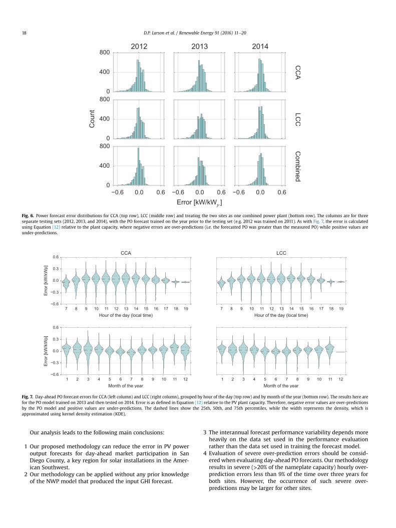
Fig. 6. Power forecast error distributions for CCA (top row), LCC (middle row) and treating the two sites as one combined power plant (bottom row). The columns are for threeseparate testing sets (2012, 2013, and 2014), with the PO forecast trained on the year prior to the testing set (e.g. 2012 was trained on 2011). As with Fig. 7, the error is calculatedusing Equation (12) relative to the plant capacity, where negative errors are over-predictions (i.e. the forecasted PO was greater than the measured PO) while positive values areunder-predictions.

Fig. 7. Day-ahead PO forecast errors for CCA (left column) and LCC (right column), grouped by hour of the day (top row) and by month of the year (bottom row). The results here arefor the PO model trained on 2013 and then tested on 2014. Error is as defined in Equation (12) relative to the PV plant capacity. Therefore, negative error values are over-predictionsby the PO model and positive values are under-predictions. The dashed lines show the 25th, 50th, and 75th percentiles, while the width represents the density, which isapproximated using kernel density estimation (KDE).

D.P. Larson et al. / Renewable Energy 91 (2016) 11e2018

Our analysis leads to the following main conclusions:

1 Our proposed methodology can reduce the error in PV poweroutput forecasts for day-ahead market participation in SanDiego County, a key region for solar installations in the Amer-ican Southwest.

2 Our methodology can be applied without any prior knowledgeof the NWP model that produced the input GHI forecast.

3 The interannual forecast performance variability depends moreheavily on the data set used in the performance evaluationrather than the data set used in training the forecast model.

4 Evaluation of severe over-prediction errors should be consid-ered when evaluating day-ahead PO forecasts. Ourmethodologyresults in severe (>20% of the nameplate capacity) hourly over-prediction errors less than 9% of the time over three years forboth sites. However, the occurrence of such severe over-predictions may be larger for other sites.

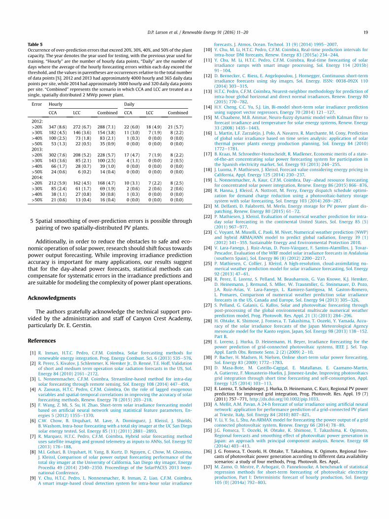
Table 5Occurrence of over-prediction errors that exceed 20%, 30%, 40%, and 50% of the plantcapacity. The year denotes the year used for testing, with the previous year used fortraining. “Hourly” are the number of hourly data points, “Daily” are the number ofdays where the average of the hourly forecasting errors within each day exceed thethreshold, and the values in parentheses are occurrences relative to the total numberof data points [%]. 2012 and 2013 had approximately 4000 hourly and 365 daily datapoints per site, while 2014 had approximately 3600 hourly and 320 daily data pointsper site. “Combined” represents the scenario in which CCA and LCC are treated as asingle, spatially distributed 2 MWp power plant.

Error Hourly Daily

CCA LCC Combined CCA LCC Combined

2012:>20% 347 (8.6) 272 (6.7) 288 (7.1) 22 (6.0) 18 (4.9) 21 (5.7)>30% 182 (4.5) 146 (3.6) 154 (3.8) 11 (3.0) 7 (1.9) 8 (2.2)>40% 100 (2.5) 73 (1.8) 83 (2.1) 1 (0.3) 0 (0.0) 0 (0.0)>50% 53 (1.3) 22 (0.5) 35 (0.9) 0 (0.0) 0 (0.0) 0 (0.0)2013:>20% 302 (7.6) 208 (5.2) 228 (5.7) 17 (4.7) 7 (1.9) 8 (2.2)>30% 143 (3.6) 85 (2.1) 100 (2.5) 4 (1.1) 0 (0.0) 2 (0.5)>40% 66 (1.7) 28 (0.7) 39 (1.0) 0 (0.0) 0 (0.0) 0 (0.0)>50% 24 (0.6) 6 (0.2) 14 (0.4) 0 (0.0) 0 (0.0) 0 (0.0)2014:>20% 212 (5.9) 162 (4.5) 168 (4.7) 10 (3.1) 7 (2.2) 8 (2.5)>30% 85 (2.4) 61 (1.7) 69 (1.9) 2 (0.6) 2 (0.6) 2 (0.6)>40% 38 (1.1) 27 (0.8) 30 (0.8) 1 (0.3) 0 (0.0) 0 (0.0)>50% 21 (0.6) 13 (0.4) 16 (0.4) 0 (0.0) 0 (0.0) 0 (0.0)

D.P. Larson et al. / Renewable Energy 91 (2016) 11e20 19

5 Spatial smoothing of over-prediction errors is possible throughpairing of two spatially-distributed PV plants.

Additionally, in order to reduce the obstacles to safe and eco-nomic operation of solar power, research should shift focus towardspower output forecasting. While improving irradiance predictionaccuracy is important for many applications, our results suggestthat for the day-ahead power forecasts, statistical methods cancompensate for systematic errors in the irradiance predictions andare suitable for modeling the complexity of power plant operations.

Acknowledgments

The authors gratefully acknowledge the technical support pro-vided by the administration and staff of Canyon Crest Academy,particularly Dr. E. Gerstin.

References

[1] R. Inman, H.T.C. Pedro, C.F.M. Coimbra, Solar forecasting methods forrenewable energy integration, Prog. Energy Combust. Sci. 6 (2013) 535e576.

[2] R. Perez, S. Kivalov, J. Schlemmer, K. Hemker Jr., D. Renn�e, T.E. Hoff, Validationof short and medium term operation solar radiation forecasts in the US, Sol.Energy 84 (2010) 2161e2172.

[3] L. Nonnenmacher, C.F.M. Coimbra, Streamline-based method for intra-daysolar forecasting through remote sensing, Sol. Energy 108 (2014) 447e459.

[4] A. Zaouras, H.T.C. Pedro, C.F.M. Coimbra, On the role of lagged exogenousvariables and spatial-temporal correlations in improving the accuracy of solarforecasting methods, Renew. Energy 78 (2015) 203e218.

[5] F. Wang, Z. Mi, S. Su, H. Zhao, Short-term solar irradiance forecasting modelbased on artificial neural network using statistical feature parameters, En-ergies 5 (2012) 1355e1370.

[6] C.W. Chow, B. Urquhart, M. Lave, A. Dominguez, J. Kleissl, J. Shields,B. Washom, Intra-hour forecasting with a total sky imager at the UC San Diegosolar energy tested, Sol. Energy 85 (11) (2011) 2881e2893.

[7] R. Marquez, H.T.C. Pedro, C.F.M. Coimbra, Hybrid solar forecasting methoduses satellite imaging and ground telemetry as inputs to ANNs, Sol. Energy 92(2013) 176e188.

[8] M.I. Gohari, B. Urquhart, H. Yang, B. Kurtz, D. Nguyen, C. Chow, M. Ghonima,J. Kleissl, Comparison of solar power output forecasting performance of thetotal sky imager at the University of California, San Diego sky imager, EnergyProcedia 49 (2014) 2340e2350. Proceedings of the SolarPACES 2013 Inter-national Conference.

[9] Y. Chu, H.T.C. Pedro, L. Nonnenmacher, R. Inman, Z. Liao, C.F.M. Coimbra,A smart image-based cloud detection system for intra-hour solar irradiance

forecasts, J. Atmos. Ocean. Technol. 31 (9) (2014) 1995e2007.[10] Y. Chu, M. Li, H.T.C. Pedro, C.F.M. Coimbra, Real-time prediction intervals for

intra-hour DNI forecasts, Renew. Energy 83 (2015a) 234e244.[11] Y. Chu, M. Li, H.T.C. Pedro, C.F.M. Coimbra, Real-time forecasting of solar

irradiance ramps with smart image processing, Sol. Energy 114 (2015b)91e104.

[12] D. Bernecker, C. Riess, E. Angelopoulou, J. Hornegger, Continuous short-termirradiance forecasts using sky images, Sol. Energy. ISSN: 0038-092X 110(2014) 303e315.

[13] H.T.C. Pedro, C.F.M. Coimbra, Nearest-neighbor methodology for prediction ofintra-hour global horizonal and direct normal irradiances, Renew. Energy 80(2015) 770e782.

[14] H.Y. Cheng, C.C. Yu, S.J. Lin, Bi-model short-term solar irradiance predictionusing support vector regressors, Energy 70 (2014) 121e127.

[15] M. Chaabene, M.B. Ammar, Neuro-fuzzy dynamic model with Kalman filter toforecast irradiance and temperature for solar energy systems, Renew. Energy33 (2008) 1435e1443.

[16] L. Martin, L.F. Zarzalejo, J. Polo, A. Navarro, R. Marchante, M. Cony, Predictionof global solar irradiance based on time series analysis: application of solarthermal power plants energy production planning, Sol. Energy 84 (2010)1772e1781.

[17] B. Kraas, M. Schroedter-Homscheidt, R. Madlener, Economic merits of a state-of-the-art concentrating solar power forecasting system for participation inthe Spanish electricity market, Sol. Energy 93 (2013) 244e255.

[18] J. Luoma, P. Mathiesen, J. Kleissl, Forecast value considering energy pricing inCalifornia, Appl. Energy 125 (2014) 230e237.

[19] L. Nonnenmacher, A. Kaur, C.F.M. Coimbra, Dayeahead resource forecastingfor concentrated solar power integration, Renew. Energy 86 (2015) 866e876.

[20] R. Hanna, J. Kleissl, A. Nottrott, M. Ferry, Energy dispatch schedule optimi-zation for demand charge reduction using a photovoltaic-battery storagesystem with solar forecasting, Sol. Energy 103 (2014) 269e287.

[21] M. Delfanti, D. Falabretti, M. Merlo, Energy storage for PV power plant dis-patching, Renew. Energy 80 (2015) 61e72.

[22] P. Mathiesen, J. Kleissl, Evaluation of numerical weather prediction for intra-day solar forecasting in the continental United States, Sol. Energy 85 (5)(2011) 967e977.

[23] C. Voyant, M. Muselli, C. Paoli, M. Nivet, Numerical weather prediction (NWP)and hybrid ARMA/ANN model to predict global radiation, Energy 39 (1)(2012) 341e355. Sustainable Energy and Environmental Protection 2010.

[24] V. Lara-Fanego, J. Ruiz-Arias, D. Pozo-V�azquez, F. Santos-Alamillos, J. Tovar-Pescador, Evaluation of the WRF model solar irradiance forecasts in Andalusia(southern Spain), Sol. Energy 86 (8) (2012) 2200e2217.

[25] P. Mathiesen, C. Collier, J. Kleissl, A high-resolution, cloud-assimilating nu-merical weather prediction model for solar irradiance forecasting, Sol. Energy92 (2013) 47e61.

[26] R. Perez, E. Lorenz, S. Pelland, M. Beauharnois, G. Van Knowe, K.J. Hemker,D. Heinemann, J. Remund, S. Mller, W. Traunmller, G. Steinmauer, D. Pozo,J.A. Ruiz-Arias, V. Lara-Fanego, L. Ramirez-Santigosa, M. Gaston-Romero,L. Pomares, Comparison of numerical weather prediction solar irradianceforecasts in the US, Canada and Europe, Sol. Energy 94 (2013) 305e326.

[27] S. Pelland, G. Galanis, G. Kallos, Solar and photovoltaic forecasting throughpost-processing of the global environmental multiscale numerical weatherprediction model, Prog. Photovolt. Res. Appl. 21 (3) (2013) 284e296.

[28] H. Ohtake, K. Shimose, J. Fonseca, T. Takashima, T. Oozeki, Y. Yamada, Accu-racy of the solar irradiance forecasts of the Japan Meteorological Agencymesoscale model for the Kanto region, Japan, Sol. Energy 98 (2013) 138e152.Part B.

[29] E. Lorenz, J. Hurka, D. Heinemann, H. Beyer, Irradiance forecasting for thepower prediction of grid-connected photovoltaic systems, IEEE J. Sel. Top.Appl. Earth Obs. Remote Sens. 2 (2) (2009) 2e10.

[30] P. Bacher, H. Madsen, H. Nielsen, Online short-term solar power forecasting,Sol. Energy 83 (2009) 1772e1783.

[31] D. Masa-Bote, M. Castillo-Cagigal, E. Matallanas, E. Caamano-Martin,A. Gutierrez, F. Monasterio-Huelin, J. Jimenez-Leube, Improving photovoltaicsgrid integration through short time forecasting and self-consumption, Appl.Energy 125 (2014) 103e113.

[32] E. Lorenz, T. Scheidsteger, J. Hurka, D. Heinemann, C. Kurz, Regional PV powerprediction for improved grid integration, Prog. Photovolt. Res. Appl. 19 (7)(2011) 757e771, http://dx.doi.org/10.1002/pip.1033.

[33] A. Mellit, A.M. Pavan, A 24-h forecast of solar irradiance using artificial neuralnetwork: application for performance prediction of a grid-connected PV plantat Trieste, Italy, Sol. Energy 84 (2010) 807e821.

[34] Y. Li, Y. Su, L. Shu, An ARMAX model for forecasting the power output of a gridconnected photovoltaic system, Renew. Energy 66 (2014) 78e89.

[35] J.G. Fonseca, T. Oozeki, H. Ohtake, K. Shimose, T. Takashima, K. Ogimoto,Regional forecasts and smoothing effect of photovoltaic power generation inJapan: an approach with principal component analysis, Renew. Energy 68(2014a) 403e413.

[36] J. G. Fonseca, T. Oozeki, H. Ohtake, T. Takashima, K. Ogimoto, Regional fore-casts of photovoltaic power generation according to different data availabilityscenarios: a study of four methods, Prog. Photovolt. Res. Appl..

[37] M. Zamo, O. Mestre, P. Arbogast, O. Pannekoucke, A benchmark of statisticalregression methods for short-term forecasting of photovoltaic electricityproduction, Part I: Deterministic forecast of hourly production, Sol. Energy105 (0) (2014a) 792e803.

D.P. Larson et al. / Renewable Energy 91 (2016) 11e2020

[38] M. Zamo, O. Mestre, P. Arbogast, O. Pannekoucke, A benchmark of statisticalregression methods for short-term forecasting of photovoltaic electricityproduction, Part II: Probabilistic forecast of daily production, Sol. Energy 105(2014b) 804e816.

[39] M.P. Almeida, O. Perpinan, L. Narvarte, PV power forecasting using anonparametric PV model, Sol. Energy 115 (2015) 354e368.

[40] A. Lacis, J. Hansen, A parameterization for the absorption of solar radiation inthe Earth's atmosphere, J. Atmos. Sci. 31 (1) (1974) 118e133.

[41] R. Marquez, C.F.M. Coimbra, Forecasting of global and direct solar irradianceusing stochastic learning methods, ground experiments and the NWS data-base, Sol. Energy 85 (2011) 746e756.

[42] R. Perez, K. Moore, S. Wilcox, D. Renne, A. Zelenka, Forecasting solar radia-tionepreliminary evaluation of an approach based upon the national forecastdatabase, Sol. Energy 81 (6) (2007) 809e812.

[43] P. Ineichen, R. Perez, A new airmass independent formulation for the Linketurbidity coefficient, Sol. Energy 73 (3) (2002) 151e157.

[44] P. Ineichen, Comparison of eight clear sky broadband models against 16

independent data banks, Sol. Energy 80 (4) (2002) 468e478.[45] C.A. Gueymard, Clear-sky irradiance predictions for solar resource mapping

and large-scale applications: improved validation methodology and detailedperformance analysis of 18 broadband radiative models, Sol. Energy 86 (8)(2012) 2145e2169.

[46] Y.M. Saint-Drenan, S. Bolfinger, R. Fritz, S. Vogt, G.H. Good, J. Dobschinski, Anempirical approach to parameterizing photovoltaic plants for power fore-casting and simulation, Sol. Energy 120 (2015) 479e493.

[47] A. Dolara, S. Leva, G. Manzolini, Comparison of different physical models forPV power output prediction, Sol. Energy 119 (2015) 83e99.

[48] C.A. Gueymard, S.M. Wilcox, Assessment of spatial and temporal variability inthe US solar resource from radiometric measurements and predictions frommodels using ground-based or satellite data, Sol. Energy 85 (2011)1068e1084.

[49] J.L. Hintze, R.D. Nelson, Violin plots: a box plot-density trace synergism, Am.Stat. 52 (2) (1998) 181e184.