NCER Working Paper SeriesNCER Working Paper Series

Forecasting day-ahead electricity load using a multiple equation time series approach

A E ClementsA E Clements A S HurnA S Hurn Z LiZ Li Working Paper #103Working Paper #103 September 2014September 2014 Revision May 2015Revision May 2015

Forecasting day-ahead electricity load using a

multiple equation time series approach

A.E. Clements, A.S. Hurn and Z. LiSchool of Economics and Finance, Queensland University of Technology.

Abstract

The quality of short-term electricity load forecasting is crucial to theoperation and trading activities of market participants in an electricitymarket. In this paper, it is shown that a multiple equation time-seriesmodel, which is estimated by repeated application of ordinary leastsquares, has the potential to match or even outperform more complexnonlinear and nonparametric forecasting models. The key ingredientof the success of this simple model is the effective use of lagged in-formation by allowing for interaction between seasonal patterns andintra-day dependencies. Although the model is built using data forthe Queensland region of Australia, the methods are completely genericand applicable to any load forecasting problem. The model’s forecast-ing ability is assessed by means of the mean absolute percentage error(MAPE). For day-ahead forecast, the MAPE returned by the modelover a period of 11 years is an impressive 1.36%. The forecast accuracyof the model is compared with a number of benchmarks including threepopular alternatives and one industrial standard reported by the Aus-tralia energy market operator (AEMO). The performance of the modeldeveloped in this paper is superior to all benchmarks and outperformsthe AEMO forecasts by about a third in terms of the MAPE criterion.

KeywordsShort-term load forecasting, seasonality, intra-day correlation, recursiveequation system.

JEL Classification NumbersC32; Q41; Q47.

Corresponding authorZili Li zili.li@connect.qut.edu.au

1 Introduction

The national electricity market (NEM) in Australia, introduced in Decem-

ber 1998, operates one of the worlds largest interconnected power systems

which comprises five regions, namely New South Wales, Victoria, Queens-

land, South Australia and Tasmania. The focus of this paper is short-term

pre-dispatch (up to 24 hours ahead) load forecasts for the Queensland re-

gion of the NEM, using half hourly data for the period from 12th July 1999

to 27th November 2013. The reasons for the importance of accurate short-

term load forecasting differ for each of the players in the market. From

the perspective of the market operator (NEM), forecasting is crucial to the

scheduling and dispatch of generation capacity; for the electricity generators,

the strategic choices involved in bidding and rebidding of capacity depend

critically on load forecasts; and for the electricity retailers, load forecasting

affects decisions about the balance between hedging and spot acquisition of

electricity. For these reasons, short-term load forecasting remains a problem

of central interest and one which has generated a large literature.

Statistical models for short-term load forecasting fall very naturally into

three main categories. First, single equation time series models model the

trajectory of load using traditional time series methods (Hagan and Behr,

1987; Darbellay and Slama, 2000; Taylor and McSharry, 2007). The efficacy

of this approach derives from the strong seasonal patterns in electricity load.

Second, and probably the current method of choice for practitioners, is the

neural network approach in which the trajectory of load is modelled semi-

parametrically using basis functions with emphasis on the non-linearity of

load (Park et al., 1991; Zhang et al., 1998; Hippert et al., 2001). Third,

multiple equation time series models have enjoyed some popularity in the

2

literature but their influence has waned in recent years. In this approach,

each period of the day (usually each half hour or hour) is treated as a

separate forecasting problem with its own equation (Peirson and Henley,

1994; Ramanathan et al., 1997; Espinoza et al., 2005; Soares and Medeiros,

2008).

The central aim of this paper is to demonstrate that the multiple equa-

tion approach has the potential to achieve a very competitive forecast ac-

curacy. The advantages of the approach are that the explanatory factors

driving forecast performance are visible, testable using traditional tests and

the fact that the model specification is linear in parameters meaning that

ordinary least squares can be used to estimate the parameters rather than

a numerical optimisation algorithm. The seminal paper on the multiple

equation approach to load forecasting is that of Ramanathan et al. (1997)

in which the advantage of the multiple equation approach was first demon-

strated in the context of the Californian electricity market. In the Australian

electricity market, a Bayesian approach is employed by Cottet and Smith

(2003) to a multiple equation model in a case study of the regional market

of New South Wales. Perhaps the most insightful multiple equation model

is that of Cancelo et al. (2008) who build a model of load in the Spanish

electricity market.

What distinguishes the proposed model in this paper from its predeces-

sors in the multiple equation time series tradition is the way in which the

daily and weekly patterns in electricity load interact and also the recognition

of the importance of intra-day correlation in load. It turns out that allow-

ing for a distinct weekly pattern in the coefficients governing one-day lagged

load is a crucial advance on previous work. The efficacy of this innovation

in dealing with seasonality is demonstrated by comparing with two tradi-

3

tional ways of dealing with seasonality, namely the double seasonal ARIMA,

the double seasonal Holt-Winters exponential smoothing approach (Gould

et al., 2008). Incorporating the proposed refinements into a multiple equa-

tion model, the forecasting performance of the final chosen model is shown

by comparing with the multiple equation model of Cancelo et al. (2008) and

a semi-parametric approach used by AEMO.

In Section 2, a prototype model representing the starting point for the

modelling exercise is developed. This model includes a piecewise linear re-

sponse of load to temperature and the development of load variations for

special days (public holidays). In Section 3, the prototype model is expanded

to capture detailed seasonality and intra-day dependency of load. Focusing

on comparing the effectiveness of modelling the seasonality of load, Section 4

compares the proposed model with two other popular alternatives. Section

5 presents the important forecasting results. The 12-hour ahead forecast

accuracy of the proposed model is compared with the forecasts from the

AEMO and an alternative multiple equation model of Cancelo et al. (2008).

Then section 6 is a brief conclusion.

2 A Prototype Multiple Equation Model

To provide a perspective on the forecasting problem addressed in this pa-

per, Figure 1, plots the average half-hourly load over a day and average

half-hourly load over the period of a week using Queensland data with the

average taken over the entire sample period from 12th July 1999 to 27th

November 2013. Diurnal and weekly patterns, both well documented fea-

tures of electricity load (Engle et al., 1989; Harvey and Koopman, 1993;

Taylor, 2010), are clearly evident. Load picks up very quickly between the

4

hours of 06:00 and 08:00 from the overnight low and remains high during the

daylight hours. The daily peak in the load profile usually occurs at 18:00

before tailing off once more. The weekly pattern in load is also quite pro-

nounced with a regular load profile evident from Monday through Thursday,

but with significant differences on Friday, Saturday and Sunday. While it is

tempting to seek to model the trajectory of load making use of these well

defined features, in fact this turns out to be a sub-optimal strategy. The

averaging process involved in computing the quantities in Figure 1 smooths

out much of the half-hourly variation in load and it is this variation that a

good forecasting model must capture.

00:00 02:00 04:00 06:00 08:00 10:00 12:00 14:00 16:00 18:00 20:00 22:00 23:004000

4500

5000

5500

6000

6500

Hours of the day

Load

(M

W)

(a)

Mon Tue Wed Thu Fri Sat Sun4000

4500

5000

5500

6000

6500

7000(b)

Days of the week

Load

(M

W)

Figure 1: Averaged half-hourly load over a day and averaged half-hourly load overa week in panels (a) and (b) respectively, for Queensland over the period from 12thJuly 1999 to 27th November 2013.

2.1 The basic model structure

A model structure that captures half-hourly variability in load while re-

specting the features of the load profile in Figure 1 is one in which each half

5

hour is modelled separately, but also uses the diurnal and other seasonal

information in the load series. Let the logarithm of the load at half hour

h and day d be given by Lh d, then, the ARMA structure of the prototype

model for a given half hour period is

Lh d =θh 0 + θh 1Lh d−1 + θh 2Lh d−7 + φh 1εh d−1 + φh 2εh d−7 + εh d ,

in which h = 1, · · · , 48 and εh d is the disturbance term. So for each half-

hour, h, the parameters are estimated based on a subset of the data which

only contains the observations at that interval. In this way, the partial

correlation between load and lagged load are allowed to differ in a daily

pattern by the different parameter values across equations. A minimal lag

structure requires Lh d to be explained by load in the same half hour on the

previous day, Lh d−1 and the load in the same half hour of the same day in

the previous week, Lh d−7. For the same reasoning, the unexpected changes

in load in the same half hour on the previous day, εh d−1 and the previous

week, εh d−7, are included.

It is important to factor in the effects of public holidays into the load

forecasting equation, something which is accomplished quite parsimoniously

using dummy variables following Cottet and Smith (2003) and Espinoza

et al. (2005). To economise on the number of parameters to estimate, these

special days are categorised into six distinct groups. Good Friday, Ester

Monday, Christmas Day and New years are the four unique special days. The

remaining two groups are a local Brisbane (the capital city of Queensland)

only holiday and all the single day public holidays. Including special day

6

variables, the prototype model becomes:

Lh d =θh 0 + θh 1Lh d−1 + θh 2Lh d−7 + φh 1εh d−1 + φh 2εh d−7 + εh d

+6∑

j=1

(αj h 1Sj h d + αj h 2Sj h d−1

),

where, Sj h d is the jth type of special day at half-hour interval h of day

d. Following (Ramanathan et al., 1997), the effect of one day lagged special

days, Sj h d−1, is also considered. The reasoning is that when the load on spe-

cial days (which is typically lower than on a normal day) is used as one day

lagged load, Lh d−1, to infer load on normal days, the effect can be suitably

adjusted. This adjustment is found to be significant and is therefore main-

tained. The effect of one week lagged special holidays is also investigated

but discounted because the improvement was found to be insignificant.

2.2 Dealing with the effect of temperature

There is some evidence to suggest that the response of load to temperature is

nonlinear in nature and the challenge is to model this nonlinear response but

at the same time maintain a model specification that is linear in parameters.

A piecewise linear specification following Cancelo et al. (2008) is adopted

with linear responses in four different temperature ranges: 9◦C - 15◦C, 9◦C

- 20◦C, 22◦C - 26◦C and 22◦C - 30◦C. Temperatures between 20◦C and

22◦C are regarded as comfortable and having no extra effect on load. Also

the temperature beyond 9◦C and 30◦C are also treated as having no extra

effect since the demand is ultimately limited by the capacity of temperature

controlling devices, an effect termed as exhaustion. If temperature in half

hour h on day d is denoted Th d, then to implement the piecewise linear

specification four variables must be constructed which represent the changes

7

in the relevant ranges of temperature. For the cooling degree temperature

ranges the following two variables are defined:

C1h d =

0 Th d ≤ 22

Th d − 22 22 < Th d ≤ 30

30 − 22 30 < Th d

, C2h d =

0 Th d ≤ 22

Th d − 26 26 < Th d ≤ 30

30 − 26 30 < Th d .

Similarly, for the heating degree temperatures another two variables are

defined:

H1h d =

0 15 ≤ Th d

15 − Th d 9 ≤ Th d < 15

15 − 9 Th d < 9

, H2h d =

0 20 ≤ Th d

20 − Th d 9 ≤ Th d < 20

20 − 9 Th d < 9

.

These variables together admit a piecewise linear response of load to tem-

perature as illustrated in Figure 2 which is similar in spirit to the flexible

spline method used by Harvey and Koopman (1993). The ranges of defined

temperature variables in which they takes non-zero values are denoted by

solid lines with arrows indicating the direction of the values which deviate

positively from zero. Also shown is a nonparametric kernel regression of the

conditional expectation of load given temperature. The nonlinear nature of

the relationship is apparent, but the piecewise linear fit appears almost iden-

tical to the nonparametric regression. The advantage of the piecewise linear

specification is that it accommodates the nonlinearity but does so within a

model that remains linear in parameters. It should be noted that different

combinations of knots for specifying temperature variable were tried in the

final version of model, but discarded in favour of the current specification.

Although, the temperature variables are included in the model, the actual

load plot in Figure 2 suggests that load varies quite widely for any given

temperature. This may be a consequence of the diverse climate in Queens-

land and the non-representative temperature record which is taken at only

one specific location.

8

Figure 2: Queensland load and temperatures, from July 1999 to December 2013.Solid line denotes a nonparametric regression fit with normal kernel and bandwidth1. Dashed line is the ordinary least squares fit with the four temperature variablesC1h d, C2h d, H1h d and H2h d. The ranges of defined temperature variables in whichthey deviate positively from zero are indicated by the arrows.

Incorporating the temperature variables into the prototype model yields

Lh d =θh 0 + θh 1Lh d−1 + θh 2Lh d−7 + φh 1εh d−1 + φh 2εh d−7 + εh d

+6∑

j=1

(αj h 1Sj h d + αj h 2Sj h d−1

)+

2∑k=1

(βk h 1Hk h d + βk h 2Ck h d + βk h 3Hk h d−1 + βk h 4Ck h d−1

). (1)

This is the preferred specification for the prototype model against which all

the refinements in later sections will be judged.

2.3 Estimating and forecasting the prototype model

The prototype model in (1) can be estimated equation-by-equation using

iterative ordinary least squares (Spliid, 1983). In the estimation, each equa-

tion is initially estimated ignoring the moving-average error terms and the

regression residuals stored. The equations are then re-estimated using the

regression residuals from the previous step as observed moving average error

9

terms. This process is then iterated until convergence which is defined as

the difference in parameter values in successive iterations being less than a

user supplied tolerance, in this case the square root of machine precision for

floating-point arithmetic.

To assess forecast performance, a 3-year rolling window of data is used for

model estimation. The day-ahead forecast is produced starting from 00:00

and uses the information available at the time of making the forecast with the

exception of the temperature variables. To avoid having to provide forecasts

for temperature, the actual data are used in all forecasting evaluations unless

specified otherwise. Moreover, as the next-day temperature forecasts are

very accurate in general, any loss in accuracy of load forecast is expected to

be very small when the actual temperature is replaced with a forecast. The

models are re-estimated every week. In total, a period of over 11 years from

July 2002 to December 2013 is used for forecast evaluation. MAPE is used

as the main criterion for assessing forecast accuracy.

00:00 02:00 04:00 06:00 08:00 10:00 12:00 14:00 16:00 18:00 20:00 22:00 23:300.3

0.5

0.7

0.9

1.1

1.3

1.5

1.7

1.9

2.1

2.3

2.5

2.7

2.9

3.1

MA

PE

Half−hourly interval

MAPE: 2.24%

Figure 3: Half-hourly MAPEs and overall MAPE for the prototype model, equa-tion (1). The overall MAPE is denoted as the solid horizontal line with its valueindicated below.

10

A summary of the forecasting results for the prototype model are re-

ported in Figure 3. The overall MAPE obtained is 2.24% with half-hourly

MAPEs during the daily peak period slightly over 3%. Figure 3 also shows a

clear daily pattern in half-hourly MAPE in which it reaches its lowest point

during the night hours, increases to a small peak at around 08:00 and then

rises continually to the daily maximum at around 16:00.

3 Extensions to the prototype model

The importance of seasonal patterns in load for accurate load forecasting

is apparent and well documented in the literature (Engle et al., 1989; Har-

vey and Koopman, 1993; Taylor, 2010). In this section two extensions to

the prototype model in (1) are proposed. The first extension addresses the

important interaction between daily and weekly load patterns, and the sec-

ond deals with intra-day load dependency by treating the equations as a

recursive system.

3.1 Addressing Seasonality

Although the design of the lag structure in equation (1) is based on observed

load profile, it does not capture completely its seasonal features. Figure 4

plots the weekly pattern in the forecast errors from the prototype model in

(1), computed by averaging the half-hourly forecasting errors over a week. It

is particularly evident that load in the half-hour intervals on Saturday and

Sunday is significantly over-predicted (negative bias in the errors). This

stems from the fact that the generally higher load on a weekday is being

used as one-day lagged load in generating the forecast for weekends. Sim-

ilarly, when Sunday load is used in generating the forecast for Monday,

significant under-prediction occurs (positive bias in the errors). Essentially

11

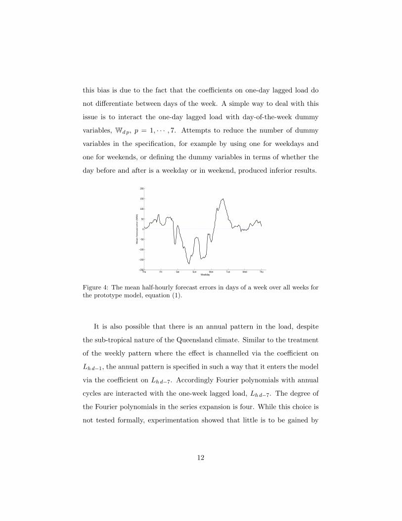
this bias is due to the fact that the coefficients on one-day lagged load do

not differentiate between days of the week. A simple way to deal with this

issue is to interact the one-day lagged load with day-of-the-week dummy

variables, Wd p, p = 1, · · · , 7. Attempts to reduce the number of dummy

variables in the specification, for example by using one for weekdays and

one for weekends, or defining the dummy variables in terms of whether the

day before and after is a weekday or in weekend, produced inferior results.

Thu Fri Sat Sun Mon Tue Wed Thu−200

−150

−100

−50

0

50

100

150

200

Me

an

fo

reca

st

err

or

(MW

)

Weekday

Figure 4: The mean half-hourly forecast errors in days of a week over all weeks forthe prototype model, equation (1).

It is also possible that there is an annual pattern in the load, despite

the sub-tropical nature of the Queensland climate. Similar to the treatment

of the weekly pattern where the effect is channelled via the coefficient on

Lh d−1, the annual pattern is specified in such a way that it enters the model

via the coefficient on Lh d−7. Accordingly Fourier polynomials with annual

cycles are interacted with the one-week lagged load, Lh d−7. The degree of

the Fourier polynomials in the series expansion is four. While this choice is

not tested formally, experimentation showed that little is to be gained by

12

increasing the degree of the polynomials.1

Incorporating the adjustments for the weekly and annual cycles gives the

extended model

Lh d =θh 0 + θh d 1Lh d−1 + θh d 2Lh d−7 + φh 1εh d−1 + φh 2εh d−7 + εh d

+6∑

j=1

(αj h 1Sj h d + αj h 2Sj h d−1

)+

2∑k=1

(βk h 1Hk h d + βk h 2Ck h d + βk h 3Hk h d−1 + βk h 4Ck h d−1

), (2)

in which:

θh d 1 =7∑

p=1

ηh pWd p ,

θh d 2 =τh 1 +

4∑q=1

[τh 2 q sin

(2qπ

( hd

17472

))+ τh 3 q cos

(2qπ

( hd

17472

))].

Forecasts obtained from this model are now evaluated using exactly the

same procedure as outlined in Section 2.3 .

The half-hourly MAPEs are shown in Figure 5 together with the MAPEs

of the prototype model. The extended model shows a significant improve-

ment over the prototype model in every half hour period and for the overall

MAPE recorded (1.56% versus 2.24%). Interestingly, it appears to be the

weekly pattern rather than the annual cycle which drives this improvement.

An overall MAPE of 1.61% was obtained from an alternative model with

only specifying the weekly interactive dummy variables. The mean half-

hourly forecast errors in days of a week obtained from the model in (2) are

shown in panel (b) of Figure 5. The weekly pattern in the forecast errors

has been largely eliminated.

1In principle, the weekly pattern previous discussed can also be modelled using Fourierpolynomials. The dummy variable specification is preferred because it allows a naturalinterpretation of the coefficient estimates.

13

00:00 02:00 04:00 06:00 08:00 10:00 12:00 14:00 16:00 18:00 20:00 22:00 23:300.30.50.70.91.11.31.51.71.92.12.32.52.72.93.1

MA

PE

(a)

Half−hourly interval

Thu Fri Sat Sun Mon Tue Wed Thu−200

−150

−100

−50

0

50

100

150

200(b)

Me

an

fo

reca

st

err

or

(MW

)

Weekday

MAPE:1.56%

Figure 5: In panel (a), the half-hourly MAPEs and overall MAPE for the prototypemodel (solid lines) in (1) are compared to the model with seasonal patterns (dashedlines) in the parameters given in (2). The overall MAPEs are shown as horizontallines with the value for equation (2) indicated below. In panel (b), the mean half-hourly forecast errors in days of a week over all weeks from the prototype model(equation (1), solid line) and the model with seasonal patterns in the parameters(equation (2), dashed line).

A more detailed breakdown of the forecast performance is provided in

Table 1. It is apparent that the most significant improvements achieved us-

ing the extended model in (2) are found in the forecasts on normal days and

weekends. The total number of large forecast errors defined as an absolute

percentage error (APE) greater than 5% is reduced by more than 10,000

instances (a 68% improvement). Overall, by interacting Lh d−1 and Lh d−7

with the weekly dummy variables and annual cycles, respectively, the overall

14

Table 1: The forecast comparison between the prototype model in (1) and themodel with seasonal patterns in the parameters (equation (2)).

Overall Maximum No. APE No. APE No. APE No. APEObs.

MAPE APE ≥ 5% ≥ 10% ≥ 15% ≥ 25%

OverallEq. (1) 2.24% 33.58% 19702 2630 430 33

199584Eq. (2) 1.56% 26.86% 6303 542 107 4

Normal Eq. (1) 2.12% 33.58% 13629 1940 322 16137232

days Eq. (2) 1.50% 24.68% 3671 266 33 0

WeekendEq. (1) 2.48% 24.75% 4912 517 61 0

57024Eq. (2) 1.62% 21.83% 2056 156 15 0

Special Eq. (1) 2.89% 32.31% 1390 243 70 176384

days Eq. (2) 2.54% 26.86% 798 186 70 4

MAPE of the forecast improves by 0.68% in comparison with the prototype

model in Section 2.

Figure 6: Estimated parameters and 95% confidence intervals (shaded areas) forweekly dummy variables in the model with seasonal patterns in the parameter(equation (2)). On the left vertical axis, the deflections of the parameter estimatesof Monday, Saturday, Sunday and other weekdays from Wednesday are denoted bydotted line with dots, dotted line with circles, dotted line with squares and solidlines respectively. On the right axis, the level of parameter estimates for Wednesdayare plotted in dashed line.

A set of representative parameter estimates for the interactive dummy

15

variables Wd p, p = 1, . . . , 7 and their 95% confidence intervals from a 3-year

rolling window estimation are plotted in Figure 6. The largest coefficient

values are seen to occur on Monday because the weekend load being used

as one day lagged load in forecasting weekday load is substantially lower

that the observed Monday load. The smallest coefficient values are found

on the weekends. This is exactly the opposite effect to that noted for Mon-

day; higher weekday loads are now being used to generate forecasts of lower

weekend loads. More interestingly, the values of the coefficients vary in dif-

ferent half hours of a day. Another discernible pattern is to be found in the

coefficients for different weekdays. In off-peak half-hourly intervals, the co-

efficients have a very similar magnitude with, in some instances, overlapping

confidence intervals across different weekdays. During peak load half-hourly

intervals, however, the values of the coefficients are substantially different

across different weekdays. This indicates clearly that there is an interaction

between daily and weekly patterns in load, a characteristic which tends to

be ignored in the load forecasting literature.

3.2 Intra-day Correlations

In the models studied thus far, the information set is defined at a daily

resolution at day d−1. One important piece of information which is ignored

is the observed load in last half-hour period of the day prior to making a

forecast, L48 d−1. This is particularly important for the first half hour period

of the forecast, as this lagged load is observed in the immediately preceding

16

half hour. Making this adjustment yields the model

Lh d =θh 0 + θh d 1Lh d−1 + θh d 2Lh d−7 + θh 4L48 d−1

+ φh 1εh d−1 + φh 2εh d−7 + εh d

+6∑

j=1

(αj h 1Sj h d + αj h 2Sj h d−1

)+

2∑k=1

(βk h 1Hk h d + βk h 2Ck h d + βk h 3Hk h d−1 + βk h 4Ck h d−1

), (3)

in which

θh d 1 =7∑

p=1

ηh pWd p ,

θh d 2 =τh 1 +4∑

q=1

[τh 2 q sin

(2qπ

( hd

17472

))+ τh,3,q cos

(2qπ

( hd

17472

))].

Figure 7 compares the MAPE of the model in (3) with the model (2)

in Section 3.1. Not surprisingly, the biggest improvement is found in the

first half-hour interval. Moreover, the substantial improvements in the half-

hourly MAPEs in the first 20 half-hour intervals indicates that this idea is

well worth pursuing a little further. Indeed, it is reasonable to posit that

the load in consecutive half hours will be correlated so that in addition to

observed load in last half-hour period of the day prior to the making a fore-

cast, L48 d−1, each equation contains the lagged load from the immediately

preceding half hour, Lh−1 d. Additional lags of consecutive half-hour periods

were tried but the improvement in forecast performance was minimal.

17

00:00 02:00 04:00 06:00 08:00 10:00 12:00 14:00 16:00 18:00 20:00 22:00 23:300.3

0.5

0.7

0.9

1.1

1.3

1.5

1.7

1.9

2.1

2.3

2.5

2.7

2.9

3.1

Half−hourly interval

MA

PE

MAPE:1.40%

Figure 7: The half-hourly MAPEs and overall MAPE for the mode with seasonalpattern in the parameters (equation (2), dashed lines) and the model with themost recent load information in (3) (dotted lines). The overall MAPEs are shownas horizontal lines with the value of which for equation (3) indicated below.

Consequently, the preferred multiple equation time series model is now

Lh d =θh 0 + θh d 1Lh d−1 + θh d 2Lh d−7 + θh 4L48 d−1 + θh 5Ih>1Lh−1 d

+ φh 1εh d−1 + φh 2εh d−7 + εh d

+6∑

j=1

(αj h 1Sj h d + αj h 2Sj h d−1

)+

2∑k=1

(βk h 1Hk h d + βk h 2Ck h d + βk h 3Hk h d−1 + βk h 4Ck h d−1

), (4)

in which

θh d 1 =

7∑p=1

ηh pWd p ,

θh d 2 =τh 1 +4∑

q=1

[τh 2 q sin

(2qπ

( hd

17472

))+ τh 3 q cos

(2qπ

( hd

17472

))],

and Ih>1 denotes an indicator function which is equal to 1 when h > 1 and

0 otherwise. This modification turns the 48 equations for the half hours of

a day into a recursive system. Once again, repeated application of ordinary

18

least squares can be used to estimate the system, it provides a parsimonious

way of capturing the intra-day load correlation without increasing compu-

tational complexity significantly. Experimentation indicates that the more

efficient estimation method with taking into account of intra-day error cor-

relation does not generally improve forecast accuracy.

The forecast results using (4) are plotted in Figure 8. Overall, the results

show that half-hourly day-ahead MAPEs are all below 2%, with an overall

MAPE of 1.36%. The improvement in forecast accuracy from using the

recursive system is mainly for the daily peak intervals between 14:00 and

18:00.

00:00 02:00 04:00 06:00 08:00 10:00 12:00 14:00 16:00 18:00 20:00 22:00 23:300.3

0.5

0.7

0.9

1.1

1.3

1.5

1.7

1.9

2.1

2.3

2.5

2.7

2.9

3.1

Half−hourly interval

MA

PE

MAPE: 1.36%

Figure 8: Forecast comparison on the half-hourly MAPEs for all the four models(solid line for equation (1), dashed line for equation (2), dotted line for equation (3)and dash-dot line for equation (4)) studied and the overall MAPE for the modelusing recursive system in (4) (dash-dot horizontal line with its value indicatedbelow).

More detailed results are reported in Table 2, in which models from (1)

to (4) are compared. It can be seen that the most significant improvement is

obtained due to the introduction of the weekly dummy variables interacting

with the lagged load, Lh d−1, in equation (2). In particular, the number of

19

instances of large errors (APE ≥ 5%) decreases by nearly 10,000 on normal

days when moving from the specification in the prototype model (1) to

the weekly dummy variable specification in (2). In addition, incorporating

the most recent information, equation (3), and using a recursive system for

intra-day correlation, equation (4), also improve accuracy but the size of

the improvement is not as large. Overall, comparing the final model in (4)

with the prototype model in (1), the reduction in the number of large APE

is over 70% in all bands, and overall MAPE drops from 2.24 % to 1.36%,

results which vindicate the modifications proposed in this section.

Table 2: The forecasting accuracy for the models studied, from equation (1) to (4).

Overall Maximum No. APE No. APE No. APE No. APEObs.

MAPE APE ≥ 5% ≥ 10% ≥ 15% ≥ 25%

Ove

rall

Eq. (1) 2.24% 33.58% 19702 2630 430 33

199584Eq. (2) 1.56% 26.86% 6303 542 107 4Eq. (3) 1.40% 25.98% 5130 467 93 4Eq. (4) 1.36% 25.70% 4499 451 95 1

Nor

mal

day

s

Eq. (1) 2.12% 33.58% 13629 1940 322 16

137232Eq. (2) 1.50% 24.68% 3671 266 33 0Eq. (3) 1.35% 24.00% 2982 216 30 0Eq. (4) 1.31% 21.62% 2544 203 31 0

Wee

ken

d Eq. (1) 2.48% 24.75% 4912 517 61 0

57024Eq. (2) 1.62% 21.83% 2056 156 15 0Eq. (3) 1.44% 21.55% 1663 143 10 0Eq. (4) 1.41% 21.77% 1521 142 13 0

Sp

ecia

ld

ays

Eq. (1) 2.89% 32.31% 1390 243 70 17

6384Eq. (2) 2.54% 26.86% 798 186 70 4Eq. (3) 2.28% 25.98% 697 168 59 4Eq. (4) 2.25% 25.70% 641 167 58 1

4 A Comparison of Approaches to Modelling Sea-sonality

The extensions proposed in Section 3 are designed to effectively model the

detailed seasonality in electricity load. In this section, the extended model

20

in equation (4) is compared with two popular methods commonly used in

the literature for dealing with seasonality. In order to focus the comparison

on modelling seasonality alone, the models in this section use only lagged

load information and all other information, such as temperature and special

days, are ignored. The two models used for comparative purposes are now

outlined.

Single equation double seasonal ARIMA model

ARIMA type models for load forecasting are widely used in the literature

(Taylor, 2012; Kim, 2013). The single equation double seasonal ARIMA

model is specified as:

φp(B)ΦP1(BS1)ΦP2(BS2)(1 −B)d(1 −BS1)D1(1 −BS2)D2(Lt − c− bt)

= θq(B)ΘQ1(BS1)ΘQ2(BS2)εt,(5)

where, B is the back shift operator. φp(B), ΦP2(BS1), ΦP2(BS2) and θq(B),

ΘQ2(BS1), ΘQ2(BS2) denote the autoregressive and moving average parts

respectively, with back shift polynomials of degree p, P1, P2 and q, Q1,

Q2 respectively and seasonal factors S1 and S2. D1, D2 are the orders of

differencing. The parameter c is the constant term and b is the parameter

for the time trend t. The model can be written as

ARIMA(p, q, d) × (P1, Q1, D1)S1 × (P2, Q2, D2)S2 .

Focusing on comparing the effectiveness of the models for modelling the

seasonality and to make the model in (5) comparable in a sense that it

uses approximately the same amount of information as used by the multiple

equation model, the specification

ARIMA(1, 1, 0) × (1, 1, 1)48 × (1, 1, 1)336 ,

21

is chosen. Depending on specific case, both the proposed multiple equa-

tion model and the single equation double seasonal ARIMA in (5) can be

easily expanded to accommodate more distant lags and other explanatory

variables.

Double seasonal Holt-Winters exponential smoothing model

In short-term load forecasting, the seasonal Holt-Winters exponential smooth-

ing (HWES) is another common choice for modelling seasonality in load

(Gould et al., 2008; De Livera et al., 2011; Taylor, 2012). An intra-day

cycles double seasonal HWES approach of (Gould et al., 2008) is imple-

mented here, which includes an unconstrained seasonal updating scheme

with 7 daily sub-cycles in a week and additive seasonal components. As

suggested by Taylor (2012), an AR(1) term for the residual is included for

better forecast accuracy. The model is specified as:

Lt = lt−1 + bt−1 + x′tst−48 + φrt−1 + εt,

rt = Lt − lt−1 − bt−1 − x′tst−48,

lt = lt−1 + bt−1 + αrt,

bt = bt−1 + βrt,

st = st−48 + Γxtrt, (6)

where lt and bt are the level and trend at time t, respectively. The variable

xt is a 7× 1 vector of day-of-the-week dummy variables, st is a 7× 1 vector

of seasonal components for the same half-hour intervals for the 7 days in a

week, rt and εt are, respectively, the residual term and an independent and

identically distributed error term with zero mean. The constants α, β are

smoothing parameters for the level and the trend, respectively, and φ is the

AR(1) parameter for the residual. The matrix Γ has dimension 7 × 7 and

22

contains the smoothing parameters for the seasonal components.

00:00 02:00 04:00 06:00 08:00 10:00 12:00 14:00 16:00 18:00 20:00 22:00 23:300

0.005

0.01

0.015

0.02

0.025

0.03

0.035

Half−hour intervals

MA

PE MAPE: 1.84% (eq. 4)

MAPE: 2.17% (eq. 8)

MAPE: 2.43% (eq. 9)

Figure 9: The half-hourly MAPEs of the one day ahead forecast produced by theproposed method (equation (4) without temperature and special days, denoted bysolid lines), the single equation double seasonal ARIMA (equation (5), denotedby dashed lines), and the unconstrained intra-day cycles double seasonal HWES(equation (6), denoted by dotted lines) from July 2002 to December 2013. Theoverall MAPEs are shown as the horizontal lines with the values indicated above.

Figure 9 plots the half-hourly MAPEs of the one-day-ahead forecasts pro-

duced by the three models for the period from July 2002 to December 2013.

The efficacy of the proposed multiple equation model for modelling season-

ality in the load is obvious. The half-hourly MAPEs and overall MAPE for

this approach are clearly lower than the corresponding forecasting statis-

tics produced by the two competitor approaches. In short, the proposed

methodology is flexible in accommodating not only daily and weekly pat-

terns of load, but also the interaction between the two in a way that leads

to a significantly improved accuracy in forecast performance as shown in

Figure 9. In the double seasonal ARIMA, neither daily nor weekly patterns

are allowed in the parameter for lagged load. In the double seasonal HWES,

23

the unconstrained seasonal component smoothing parameters, Γ allow the

seasonal component for a half-hour interval in a day of a week to be updated

based on the observed load at the same half-hour interval in other days of a

week, but the intra-day smoothing parameter is assumed to be fixed.

5 Assessing Forecast Performance of the Full Model

In this section, the forecast performance of the preferred model in (4) is

compared against the industry standard reported by the market operator

AEMO. AEMO as the operator of the NEM, provides short-term load fore-

casts in pre-dispatch IS reports for the next trading day.2 Among the

horizons of the load forecast, 12-hour ahead forecasts provide important

information for dispatch planning for the next day. To monitor 12-hour

ahead load forecast accuracy, the monthly averaged MAPE of the 12-hour

ahead forecasts is reported by AEMO as a benchmark for assessing the

forecasting performance.3 Although the details of the specification of the

AEMO forecasting procedure are not available, it is known to be based on

the semi-parametric specification of Fan and Hyndman (2012) and as the

main forecasting model chosen by the market operator, may be taken to be

representative of the state of art performance of load forecasting models.4

The model is also compared with the multiple equation model proposed

by Cancelo et al. (2008), hereafter CEG. In this model, the seasonality

of load is dealt with using a seasonal ARIMA process, which results in a

non-linear model specification requiring estimation by maximum likelihood.

2See, http://www.nemweb.com.au/REPORTS/CURRENT/PreDispatchIS_Reports/.3See,http://www.aemo.com.au/Electricity/Data/PreDispatch-Demand-

Forecasting-Performance4See, http://www.aemo.com.au/Electricity/Planning/Forecasting/National-

Electricity-Forecasting-Report-2012

24

Forecasting of the models is implemented using an identical procedure and

the same set of variables defined in Section 2.3. To align with the 12-hour

ahead forecast accuracy reported by AEMO, the accuracy of the proposed

model (4) and CEG are assessed using 12-hour ahead forecasts.

00:00 02:00 04:00 06:00 08:00 10:00 12:00 14:00 16:00 18:00 20:00 22:00 23:300.3

0.5

0.7

0.9

1.1

1.3

1.5

1.7

1.9

2.1

2.3

2.5

2.7

2.9

3.1

Half−hourly interval

MA

PE

MAPE:1.61%

MAPE: 1.13%

Figure 10: The half-hourly MAPEs of 12-hour ahead forecast by equation (4) (solidlines) and CEG (dashed lines) from July 2002 to December 2013. The overallMAPEs are shown as the horizontal lines.

A first comparison involves only the preferred model, (4), and CEG

given that the AEMO forecast errors are only available for a shorter period.

Forecasts of the two multiple equation models are generated using the same

procedure as in Section 2.3 and the results are illustrated in Figure 10. It

can been seen that the forecast accuracy of proposed model (4) is superior

to that of CEG. An important anomaly in the CEG model is that it only

utilizes information available 24 hours previously in making a forecast. This

is clearly a flaw because it does not allow the model to be flexible in terms

of forecasting for periods less than 24 hours. Even in the first 12 hours when

forecasts from the two models are based on the same available information,

the lower MAPEs obtained from proposed model (4) shows the advantages

25

of using the latest observed load together with the recursive structure de-

veloped in Section 3.2. Note that in the case of 12-hour ahead forecasts,

the variable L48 d−1 in (4) is replaced with Lh d = Ih≤24L48 d−1 + Ih>24L24 d.

This is responsible for the marked decrease in half-hourly MAPEs shown

in Figure 10 starting from 12:00 when the most recent load information is

updated. A more detailed comparison of the performance of the two mod-

els is shown in columns 2 and 3 of Table 3 where CEG produces inferior

forecasts under all criteria. Since CEG only utilize information at a daily

resolution, the results shown in column 2 for the CEG forecasts over the

whole period can also be compared with the 24-hour ahead forecast from

model (4) shown in row 5 of Table 2. The 1.36% overall MAPE of proposed

model (4) is 0.25% lower than the one obtained from CEG (1.61%) and

similar superior performance of the former is observed in all the criteria.

Table 3: Summary comparison of 12-hours ahead forecast by equation (4), CEGand the AEMO forecasts.

Jul 2002 - Dec 2013 Jul 2012 - Nov 2013

CEG Eq. (4) CEG Eq. (4)Eq. (4) without AEMO

temperature forecasts

Overall MAPE 1.61% 1.13% 1.67% 1.21% 1.37% 1.88%Max. APE 27.99% 25.68% 20.89% 20.21% 20.26% -No. APE ≥ 5% 6981 2009 1092 384 585 -No. APE ≥ 10% 645 205 128 38 44 -No. APE ≥ 15% 120 45 27 7 7 -No. APE ≥ 25% 3 3 0 0 0 -Max. monthly MAPE - - 2.99% 1.84% 2.02% 3.2%Obs. 199584 199584 24864 24864 24864 -

Given the limited historical data publicly available from AEMO, the

period from July 2012 to November 2013 is used for subsequent compari-

son. Although this period is only 17 months, the advantage of the proposed

model is shown clearly in Figure 11 and columns 4 to 7 of Table 3, with the

26

Jul Aug Sep Oct Nov Dec Jan Feb Mar Apr May Jun Jul Aug Sep Oct Nov0.5

0.7

0.9

1.1

1.3

1.5

1.7

1.9

2.1

2.3

2.5

2.7

2.9

3.1

Month

MAP

E

Figure 11: 12-hours ahead forecasts comparison of monthly MAPE between equa-tion (4) (solid line), equation (4) without the future temperature (dotted line), CEG(dashed line) and the AEMO forecast (dot-dash line), from July 2012 to November2013.

monthly MAPEs well below the AEMO forecasts and an improvement of

around 0.67% in the overall MAPE over the AMEO forecasts. Since AEMO

forecasts are based on temperature forecasts instead of real temperature, the

results from the proposed model obtained by omitting the variables for cur-

rent temperature are also reported. While there is a fall in accuracy relative

to the situation when actual temperature is used, Figure 11 demonstrates

that this effect is very small and the model is still more accurate than the

AEMO forecast under all criteria (0.51% lower in the overall MAPE). The

advantage of model (4) over CEG (which uses actual temperature data in

the forecast) is also shown in Figure 11 and columns 4 to 6 of Table 3, where

either with or without actual temperature, the preferred model is seen to

outperform CEG under all criteria.

27

6 Conclusion

The problem of forecasting load is an important one for all electricity mar-

ket participants because it informs their strategic decisions about dispatch

(market operators), bidding and rebidding (generators) and trading activity

(retailers). In recent times a consensus seems to have developed that neu-

ral network or non-parametric based forecasts of load, with their inherently

nonlinear structure, offer the best alternative for accurate forecasting. This

paper has demonstrated that a traditional time-series approach, in which

an equation is specified for each half hour of the day, provides a viable al-

ternative method which produces very competitive results if implemented

carefully.

The multiple equation load forecasting model in this paper pays partic-

ular attention to the interaction between daily and weekly load patterns.

Probably the most important distinguishing factor in the proposed model

relative to others in the literature is the flexibility built into the influence of

load from the same half hour on the previous day. Allowing the strong weekly

pattern to interact with the daily pattern in coefficients on lagged load yields

important improvements in short-term forecast performance. Another in-

novative dimension of the current model is the use of the inherent recursive

structure of the model to capture the intra-day load correlation. The ef-

fectiveness of the proposed approach on modelling the seasonal features of

electricity load is demonstrated by comparing with two popular alternatives,

double seasonal ARIMA and Holt-Winters exponential smoothing. Despite

these modifications to the preferred model, it remains linear in parameters

and can be estimated equation-by-equation by ordinary least squares.

Overall, the forecasting performance of the preferred model is impressive

28

and significantly out-performs two benchmarks with which it is compared.

In particular, the model improves on the mean average percentage error

of 12-hour ahead forecast reported by the Australian energy market oper-

ator by about a third. For the entire 11 year period, the model returns a

mean average percentage error of 1.36% on half-hourly day-ahead forecasts,

a figure is lower than most (if not all) comparable average error statistics

reported in the literature. Of course, the simple computation of an error

metric does not really encapsulate the economic advantage to market par-

ticipants of providing accurate load forecasts. The challenge for future work

is to devise a metric that is capable of measuring economic gains to more

accurate load forecasting.

References

Cancelo, J. R., Espasa, A., and Grafe, R. 2008. Forecasting the electricity

load from one day to one week ahead for the Spanish system operator.

International Journal of Forecasting, 24(4), 588–602.

Cottet, R., and Smith, M. 2003. Bayesian Modeling and Forecasting of In-

traday Electricity Load. Journal of the American Statistical Association,

98(464), 839–849.

Darbellay, G. A., and Slama, M. 2000. Forecasting the short-term demand

for electricity: Do neural networks stand a better chance? International

Journal of Forecasting, 16(1), 71–83.

De Livera, A. M., Hyndman, R. J., and Snyder, R. D. 2011. Forecasting Time

Series With Complex Seasonal Patterns Using Exponential Smoothing.

Journal of the American Statistical Association, 106(496), 1513–1527.

29

Engle, R. F., Granger, C. W. J., and Hallman, J. J. 1989. Merging short-and

long-run forecasts: An application of seasonal cointegration to monthly

electricity sales forecasting. Journal of Econometrics, 40(1), 45–62.

Espinoza, M., Joye, C., Belmans, R., and De Moor, B. 2005. Short-Term

Load Forecasting, Profile Identification, and Customer Segmentation: A

Methodology Based on Periodic Time Series. IEEE Transactions on

Power Systems, 20(3), 1622–1630.

Fan, S., and Hyndman, R.J. 2012. Short-Term Load Forecasting Based on a

Semi-Parametric Additive Model. IEEE Transactions on Power Systems,

27(1), 134–141.

Gould, Phillip G., Koehler, Anne B., Ord, J. Keith, Snyder, Ralph D.,

Hyndman, Rob J., and Vahid-Araghi, Farshid. 2008. Forecasting time

series with multiple seasonal patterns. European Journal of Operational

Research, 191(1), 207–222.

Hagan, M. T., and Behr, S. M. 1987. The Time Series Approach to Short

Term Load Forecasting. IEEE Transactions on Power Systems, 2(3),

785–791.

Harvey, A., and Koopman, S. J. 1993. Forecasting Hourly Electricity De-

mand Using Time-Varying Splines. Journal of the American Statistical

Association, 88(424), 1228–1236.

Hippert, H. S., Pedreira, C. E., and Souza, R. C. 2001. Neural networks for

short-term load forecasting: A review and evaluation. IEEE Transactions

on Power Systems, 16(1), 44–55.

30

Kim, M. S. 2013. Modeling special-day effects for forecasting intraday elec-

tricity demand. European Journal of Operational Research, 230(1), 170–

180.

Park, D. C., El-Sharkawi, M. A., Marks, R. J., Atlas, L. E., and Damborg,

M. J. 1991. Electric load forecasting using an artificial neural network.

IEEE Transactions on Power Systems, 6(2), 442–449.

Peirson, J., and Henley, A. 1994. Electricity load and temperature: Issues

in dynamic specification. Energy Economics, 16(4), 235–243.

Ramanathan, R., Engle, R., Granger, C. W. J., Vahid-Araghi, F., and Brace,

C. 1997. Shorte-run forecasts of electricity loads and peaks. International

Journal of Forecasting, 13(2), 161–174.

Soares, L. J., and Medeiros, M. C. 2008. Modeling and forecasting short-

term electricity load: A comparison of methods with an application to

Brazilian data. International Journal of Forecasting, 24(4), 630–644.

Spliid, H. 1983. A Fast Estimation Method for the Vector Autoregressive

Moving Average Model With Exogenous Variables. Journal of the Amer-

ican Statistical Association, 78(384), 843–849.

Taylor, J. W. 2010. Triple seasonal methods for short-term electricity de-

mand forecasting. European Journal of Operational Research, 204(1),

139–152.

Taylor, J. W., and McSharry, P. E. 2007. Short-Term Load Forecasting

Methods: An Evaluation Based on European Data. IEEE Transactions

on Power Systems, 22(4), 2213–2219.

31

Taylor, J.W. 2012. Short-Term Load Forecasting With Exponentially

Weighted Methods. IEEE Transactions on Power Systems, 27(1), 458–

464.

Zhang, G., Eddy Patuwo, B., and Hu, M. Y. 1998. Forecasting with ar-

tificial neural networks:: The state of the art. International Journal of

Forecasting, 14(1), 35–62.

32