forecasting electricity demand distributions using a
TRANSCRIPT

Forecasting electricity demanddistributions using asemiparametric additive model
Rob J Hyndman
Joint work with Shu FanForecasting electricity demand distributions 1

Outline
1 The problem
2 The model
3 Long-term forecasts
4 Short term forecasts
Forecasting electricity demand distributions The problem 2

The problem in 2007
We want to forecast the peak electricitydemand in a half-hour period in ten years time.
We have twelve years of half-hourly electricitydata, temperature data and some economicand demographic data.
The location is South Australia: home to themost volatile electricity demand in the world.
Sounds impossible?
Forecasting electricity demand distributions The problem 3

South Australian demand data
Forecasting electricity demand distributions The problem 4

South Australian demand data
Forecasting electricity demand distributions The problem 4
South Australia state wide demand (winter 09/10)
Sou
th A
ustr
alia
sta
te w
ide
dem
and
(GW
)
1.5
2.0
2.5
Jul 09 Aug 09 Sept 09 Apr 10 May 10 June 10

South Australian demand data
Forecasting electricity demand distributions The problem 4

South Australian demand data
Forecasting electricity demand distributions The problem 4
Black Saturday→

South Australian demand data
Forecasting electricity demand distributions The problem 4
South Australia state wide demand (summer 10/11)
Sou
th A
ustr
alia
sta
te w
ide
dem
and
(GW
)
1.5
2.0
2.5
3.0
3.5
Oct 10 Nov 10 Dec 10 Jan 11 Feb 11 Mar 11

South Australian demand data
Forecasting electricity demand distributions The problem 4
South Australia state wide demand (January 2011)
Date in January
Sou
th A
ustr
alia
n de
man
d (G
W)
1.5
2.0
2.5
3.0
3.5
1 3 5 7 9 11 13 15 17 19 21 23 25 27 29 3111 13 15 17 19 21

Demand boxplots (Sth Aust)
Forecasting electricity demand distributions The problem 5

Temperature data (Sth Aust)
Forecasting electricity demand distributions The problem 6

Demand densities (Sth Aust)
Forecasting electricity demand distributions The problem 7

Outline
1 The problem
2 The model
3 Long-term forecasts
4 Short term forecasts
Forecasting electricity demand distributions The model 8

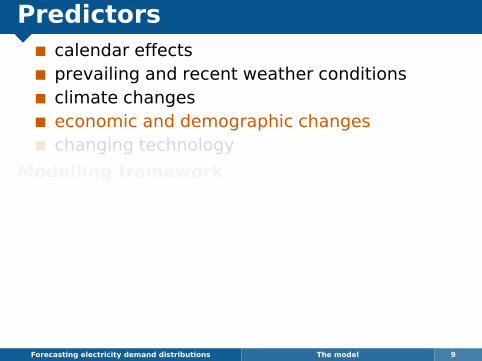
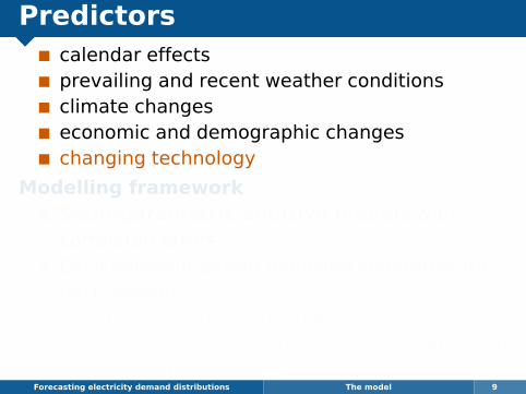
Predictorscalendar effectsprevailing and recent weather conditionsclimate changeseconomic and demographic changeschanging technology
Modelling frameworkSemi-parametric additive models withcorrelated errors.Each half-hour period modelled separately foreach season.Variables selected to provide bestout-of-sample predictions using cross-validationon each summer.
Forecasting electricity demand distributions The model 9

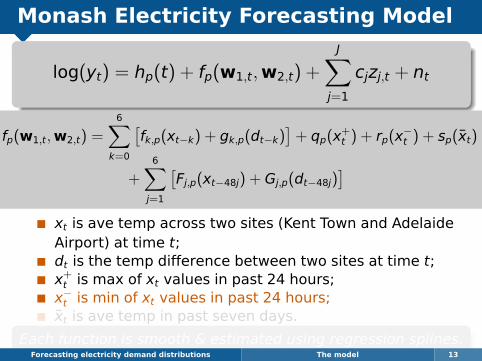
Monash Electricity Forecasting Model
log(yt) = hp(t) + fp(w1,t,w2,t) +
J∑j=1
cjzj,t + nt
yt denotes per capita demand (minus offset) at time t(measured in half-hourly intervals) and p denotes thetime of day p = 1, . . . ,48;
hp(t) models all calendar effects;
fp(w1,t,w2,t) models all temperature effects where w1,t isa vector of recent temperatures at location 1 and w2,t isa vector of recent temperatures at location 2;
zj,t is a demographic or economic variable at time t
nt denotes the model error at time t.
Forecasting electricity demand distributions The model 10

Monash Electricity Forecasting Model
log(yt) = hp(t) + fp(w1,t,w2,t) +
J∑j=1
cjzj,t + nt
hp(t) includes handle annual, weekly and daily seasonalpatterns as well as public holidays:
hp(t) = `p(t) + αt,p + βt,p + γt,p + δt,p
`p(t) is “time of summer” effect (a regression spline);
αt,p is day of week effect;
βt,p is “holiday” effect;
γt,p New Year’s Eve effect;
δt,p is millennium effect;
Forecasting electricity demand distributions The model 11

Fitted results (Summer 3pm)
Forecasting electricity demand distributions The model 12
0 50 100 150
−0.
40.
00.
4
Day of summer
Effe
ct o
n de
man
d
Mon Tue Wed Thu Fri Sat Sun
−0.
40.
00.
4
Day of week
Effe
ct o
n de
man
d
Normal Day before Holiday Day after
−0.
40.
00.
4
Holiday
Effe
ct o
n de
man
d
Time: 3:00 pm

Monash Electricity Forecasting Model
log(yt) = hp(t) + fp(w1,t,w2,t) +
J∑j=1
cjzj,t + nt
fp(w1,t,w2,t) =6∑
k=0
[fk,p(xt−k) + gk,p(dt−k)
]+ qp(x+
t ) + rp(x−t ) + sp(xt)
+6∑j=1
[Fj,p(xt−48j) + Gj,p(dt−48j)
]xt is ave temp across two sites (Kent Town and AdelaideAirport) at time t;dt is the temp difference between two sites at time t;x+t is max of xt values in past 24 hours;x−t is min of xt values in past 24 hours;xt is ave temp in past seven days.
Each function is smooth & estimated using regression splines.Forecasting electricity demand distributions The model 13

Fitted results (Summer 3pm)
Forecasting electricity demand distributions The model 14
10 20 30 40
−0.
4−
0.2
0.0
0.2
0.4
Temperature
Effe
ct o
n de
man
d
10 20 30 40
−0.
4−
0.2
0.0
0.2
0.4
Lag 1 temperature
Effe
ct o
n de
man
d
10 20 30 40
−0.
4−
0.2
0.0
0.2
0.4
Lag 2 temperature
Effe
ct o
n de
man
d
10 20 30 40
−0.
4−
0.2
0.0
0.2
0.4
Lag 3 temperature
Effe
ct o
n de
man
d
10 20 30 40
−0.
4−
0.2
0.0
0.2
0.4
Lag 1 day temperature
Effe
ct o
n de
man
d
10 15 20 25 30
−0.
4−
0.2
0.0
0.2
0.4
Last week average temp
Effe
ct o
n de
man
d
15 25 35
−0.
4−
0.2
0.0
0.2
0.4
Previous max temp
Effe
ct o
n de
man
d
10 15 20 25
−0.
4−
0.2
0.0
0.2
0.4
Previous min temp
Effe
ct o
n de
man
d
Time: 3:00 pm

Monash Electricity Forecasting Model
log(yt) = hp(t) + fp(w1,t,w2,t) +
J∑j=1
cjzj,t + nt
Other variables described by linearrelationships with coefficients c1, . . . , cJ.Estimation based on annual data.
Forecasting electricity demand distributions The model 15

Monash Electricity Forecasting Model
log(yt) = hp(t) + fp(w1,t,w2,t) +
J∑j=1
cjzj,t + nt
Other variables described by linearrelationships with coefficients c1, . . . , cJ.Estimation based on annual data.
Forecasting electricity demand distributions The model 15
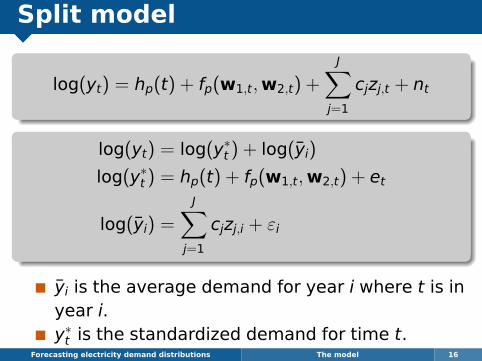
Split model
log(yt) = hp(t) + fp(w1,t,w2,t) +
J∑j=1
cjzj,t + nt
log(yt) = log(y∗t ) + log(yi)
log(y∗t ) = hp(t) + fp(w1,t,w2,t) + et
log(yi) =
J∑j=1
cjzj,i + εi
yi is the average demand for year i where t is inyear i.y∗t is the standardized demand for time t.
Forecasting electricity demand distributions The model 16

Split model
Forecasting electricity demand distributions The model 17

Split model
Forecasting electricity demand distributions The model 17

Annual model
log(yi) =∑j
cjzj,i + εi
log(yi)− log(yi−1) =∑j
cj(zj,i − zj,i−1) + ε∗i
First differences modelled to avoidnon-stationary variables.Predictors: Per-capita GSP, Price, Summer CDD,Winter HDD.
Forecasting electricity demand distributions The model 18

Annual model
log(yi) =∑j
cjzj,i + εi
log(yi)− log(yi−1) =∑j
cj(zj,i − zj,i−1) + ε∗i
First differences modelled to avoidnon-stationary variables.Predictors: Per-capita GSP, Price, Summer CDD,Winter HDD.
Forecasting electricity demand distributions The model 18

Annual model
log(yi) =∑j
cjzj,i + εi
log(yi)− log(yi−1) =∑j
cj(zj,i − zj,i−1) + ε∗i
First differences modelled to avoidnon-stationary variables.Predictors: Per-capita GSP, Price, Summer CDD,Winter HDD.
zCDD =∑
summer
max(0, T − 18.5)
T = daily mean
Forecasting electricity demand distributions The model 18

Annual model
log(yi) =∑j
cjzj,i + εi
log(yi)− log(yi−1) =∑j
cj(zj,i − zj,i−1) + ε∗i
First differences modelled to avoidnon-stationary variables.Predictors: Per-capita GSP, Price, Summer CDD,Winter HDD.
zHDD =∑
winter
max(0,18.5− T)
T = daily mean
Forecasting electricity demand distributions The model 18

Annual model
Cooling and Heating Degree Days20
040
060
0
scdd
850
950
1050
1990 1995 2000 2005 2010
whd
d
Year
Cooling and Heating degree days
Forecasting electricity demand distributions The model 19
Annual model
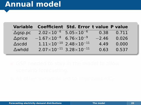
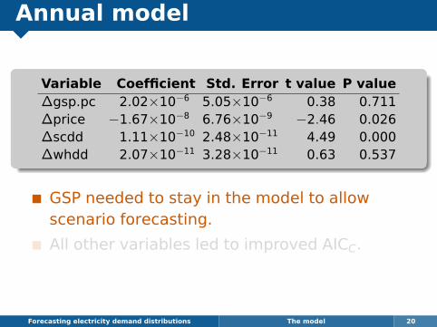
Variable Coefficient Std. Error t value P value∆gsp.pc 2.02×10⁻⁶ 5.05×10⁻⁶ 0.38 0.711∆price −1.67×10⁻⁸ 6.76×10⁻⁹ −2.46 0.026∆scdd 1.11×10⁻¹⁰ 2.48×10⁻¹¹ 4.49 0.000∆whdd 2.07×10⁻¹¹ 3.28×10⁻¹¹ 0.63 0.537
GSP needed to stay in the model to allowscenario forecasting.
All other variables led to improved AICC.
Forecasting electricity demand distributions The model 20
Annual model
Variable Coefficient Std. Error t value P value∆gsp.pc 2.02×10⁻⁶ 5.05×10⁻⁶ 0.38 0.711∆price −1.67×10⁻⁸ 6.76×10⁻⁹ −2.46 0.026∆scdd 1.11×10⁻¹⁰ 2.48×10⁻¹¹ 4.49 0.000∆whdd 2.07×10⁻¹¹ 3.28×10⁻¹¹ 0.63 0.537
GSP needed to stay in the model to allowscenario forecasting.
All other variables led to improved AICC.
Forecasting electricity demand distributions The model 20

Annual model
Forecasting electricity demand distributions The model 21
Year
Ann
ual d
eman
d
1.0
1.1
1.2
1.3
1.4
1.5
1.6
1.7
89/90 91/92 93/94 95/96 97/98 99/00 01/02 03/04 05/06 07/08 09/10
ActualFitted

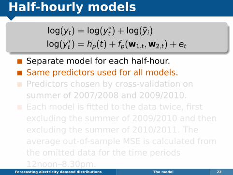
Half-hourly models
log(yt) = log(y∗t ) + log(yi)
log(y∗t ) = hp(t) + fp(w1,t,w2,t) + et
Separate model for each half-hour.Same predictors used for all models.Predictors chosen by cross-validation onsummer of 2007/2008 and 2009/2010.Each model is fitted to the data twice, firstexcluding the summer of 2009/2010 and thenexcluding the summer of 2010/2011. Theaverage out-of-sample MSE is calculated fromthe omitted data for the time periods12noon–8.30pm.
Forecasting electricity demand distributions The model 22

Half-hourly modelsx x1 x2 x3 x4 x5 x6 x48 x96 x144 x192 x240 x288 d d1 d2 d3 d4 d5 d6 d48 d96 d144 d192 d240 d288 x+ x− x dow hol dos MSE
1 • • • • • • • • • • • • • • • • • • • • • • • • • • • • • • • • 1.0372 • • • • • • • • • • • • • • • • • • • • • • • • • • • • • • • 1.0343 • • • • • • • • • • • • • • • • • • • • • • • • • • • • • • 1.0314 • • • • • • • • • • • • • • • • • • • • • • • • • • • • • 1.0275 • • • • • • • • • • • • • • • • • • • • • • • • • • • • 1.0256 • • • • • • • • • • • • • • • • • • • • • • • • • • • 1.0207 • • • • • • • • • • • • • • • • • • • • • • • • • • 1.0258 • • • • • • • • • • • • • • • • • • • • • • • • • • 1.0269 • • • • • • • • • • • • • • • • • • • • • • • • • 1.035
10 • • • • • • • • • • • • • • • • • • • • • • • • 1.04411 • • • • • • • • • • • • • • • • • • • • • • • 1.05712 • • • • • • • • • • • • • • • • • • • • • • 1.07613 • • • • • • • • • • • • • • • • • • • • • 1.10214 • • • • • • • • • • • • • • • • • • • • • • • • • • 1.01815 • • • • • • • • • • • • • • • • • • • • • • • • • 1.02116 • • • • • • • • • • • • • • • • • • • • • • • • 1.03717 • • • • • • • • • • • • • • • • • • • • • • • 1.07418 • • • • • • • • • • • • • • • • • • • • • • 1.15219 • • • • • • • • • • • • • • • • • • • • • 1.18020 • • • • • • • • • • • • • • • • • • • • • • • • • 1.02121 • • • • • • • • • • • • • • • • • • • • • • • • 1.02722 • • • • • • • • • • • • • • • • • • • • • • • 1.03823 • • • • • • • • • • • • • • • • • • • • • • 1.05624 • • • • • • • • • • • • • • • • • • • • • 1.08625 • • • • • • • • • • • • • • • • • • • • 1.13526 • • • • • • • • • • • • • • • • • • • • • • • • • 1.00927 • • • • • • • • • • • • • • • • • • • • • • • • • 1.06328 • • • • • • • • • • • • • • • • • • • • • • • • • 1.02829 • • • • • • • • • • • • • • • • • • • • • • • • • 3.52330 • • • • • • • • • • • • • • • • • • • • • • • • • 2.14331 • • • • • • • • • • • • • • • • • • • • • • • • • 1.523
Forecasting electricity demand distributions The model 23

Half-hourly models
Forecasting electricity demand distributions The model 24
6070
8090
R−squared
Time of day
R−
squa
red
(%)
12 midnight 6:00 am 9:00 am 12 noon 3:00 pm 6:00 pm 9:00 pm3:00 am 12 midnight

Half-hourly models
Forecasting electricity demand distributions The model 24
South Australian demand (January 2011)
Date in January
Sou
th A
ustr
alia
n de
man
d (G
W)
1.0
1.5
2.0
2.5
3.0
3.5
4.0
1 3 5 7 9 11 13 15 17 19 21 23 25 27 29 31
ActualFitted
Temperatures (January 2011)
Date in January
Tem
pera
ture
(de
g C
)
1015
2025
3035
4045
1 3 5 7 9 11 13 15 17 19 21 23 25 27 29 31
Kent TownAirport

Half-hourly models
Forecasting electricity demand distributions The model 24

Half-hourly models
Forecasting electricity demand distributions The model 24

Adjusted model
Original model
log(yt) = hp(t) + fp(w1,t,w2,t) +
J∑j=1
cjzj,t + nt
Model allowing saturated usage
qt = hp(t) + fp(w1,t,w2,t) +
J∑j=1
cjzj,t + nt
log(yt) =
{qt if qt ≤ τ ;τ + k(qt − τ) if qt > τ .
Forecasting electricity demand distributions The model 25

Adjusted model
Original model
log(yt) = hp(t) + fp(w1,t,w2,t) +
J∑j=1
cjzj,t + nt
Model allowing saturated usage
qt = hp(t) + fp(w1,t,w2,t) +
J∑j=1
cjzj,t + nt
log(yt) =
{qt if qt ≤ τ ;τ + k(qt − τ) if qt > τ .
Forecasting electricity demand distributions The model 25

Outline
1 The problem
2 The model
3 Long-term forecasts
4 Short term forecasts
Forecasting electricity demand distributions Long-term forecasts 26

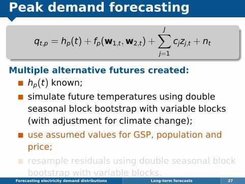
Peak demand forecasting
qt,p = hp(t) + fp(w1,t,w2,t) +
J∑j=1
cjzj,t + nt
Multiple alternative futures created:hp(t) known;
simulate future temperatures using doubleseasonal block bootstrap with variable blocks(with adjustment for climate change);
use assumed values for GSP, population andprice;
resample residuals using double seasonal blockbootstrap with variable blocks.
Forecasting electricity demand distributions Long-term forecasts 27

Seasonal block bootstrapping
Conventional seasonal block bootstrap
Same as block bootstrap but with whole years as theblocks to preserve seasonality.But we only have about 10–15 years of data, so there is alimited number of possible bootstrap samples.
Double seasonal block bootstrap
Suitable when there are two seasonal periods (here wehave years of 151 days and days of 48 half-hours).Divide each year into blocks of length 48m.Block 1 consists of the first m days of the year, block 2consists of the next m days, and so on.Bootstrap sample consists of a sample of blocks whereeach block may come from a different randomly selectedyear but must be at the correct time of year.
Forecasting electricity demand distributions Long-term forecasts 28

Seasonal block bootstrapping
Forecasting electricity demand distributions Long-term forecasts 29
Actual temperatures
Days
degr
ees
C
0 10 20 30 40 50 60
1015
2025
3035
40
Bootstrap temperatures (fixed blocks)
Days
degr
ees
C
0 10 20 30 40 50 60
1015
2025
3035
40
Bootstrap temperatures (variable blocks)
Days
degr
ees
C
0 10 20 30 40 50 60
1015
2025
3035
40

Seasonal block bootstrapping
Problems with the double seasonal bootstrapBoundaries between blocks can introduce largejumps. However, only at midnight.Number of values that any given time in year isstill limited to the number of years in the dataset.
Forecasting electricity demand distributions Long-term forecasts 30

Seasonal block bootstrapping
Variable length double seasonal blockbootstrap
Blocks allowed to vary in length between m−∆and m + ∆ days where 0 ≤ ∆ < m.Blocks allowed to move up to ∆ days from theiroriginal position.Has little effect on the overall time seriespatterns provided ∆ is relatively small.Use uniform distribution on (m−∆,m + ∆) toselect block length, and independent uniformdistribution on (−∆,∆) to select variation onstarting position for each block.
Forecasting electricity demand distributions Long-term forecasts 31

Seasonal block bootstrapping
Forecasting electricity demand distributions Long-term forecasts 32
Actual temperatures
Days
degr
ees
C0 10 20 30 40 50 60
1015
2025
3035
40
Bootstrap temperatures (fixed blocks)
Days
degr
ees
C
0 10 20 30 40 50 60
1015
2025
3035
40
Bootstrap temperatures (variable blocks)
Days
degr
ees
C
0 10 20 30 40 50 60
1015
2025
3035
40

Seasonal block bootstrapping
Forecasting electricity demand distributions Long-term forecasts 32

Peak demand forecasting
qt,p = hp(t) + fp(w1,t,w2,t) +
J∑j=1
cjzj,t + nt
Multiple alternative futures created:hp(t) known;simulate future temperatures using doubleseasonal block bootstrap with variableblocks (with adjustment for climate change);use assumed values for GSP, population andprice;resample residuals using double seasonal blockbootstrap with variable blocks.
Forecasting electricity demand distributions Long-term forecasts 33
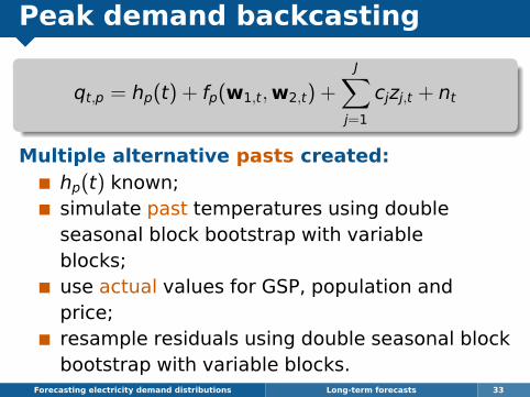
Peak demand backcasting
qt,p = hp(t) + fp(w1,t,w2,t) +
J∑j=1
cjzj,t + nt
Multiple alternative pasts created:hp(t) known;simulate past temperatures using doubleseasonal block bootstrap with variableblocks;use actual values for GSP, population andprice;resample residuals using double seasonal blockbootstrap with variable blocks.
Forecasting electricity demand distributions Long-term forecasts 33

Estimated historical quantiles
Forecasting electricity demand distributions Long-term forecasts 34
PoE (annual interpretation)
Year
PoE
Dem
and
2.0
2.5
3.0
3.5
4.0
98/99 00/01 02/03 04/05 06/07 08/09 10/11
10 %50 %90 %
●
●
●
●
●
●
●●
● ●
●
●
●
●

Peak demand forecasting
qt,p = hp(t) + fp(w1,t,w2,t) +
J∑j=1
cjzj,t + nt
Multiple alternative futures created:hp(t) known;simulate future temperatures using doubleseasonal block bootstrap with variableblocks (with adjustment for climate change);use assumed values for GSP, population andprice;resample residuals using double seasonal blockbootstrap with variable blocks.
Forecasting electricity demand distributions Long-term forecasts 35
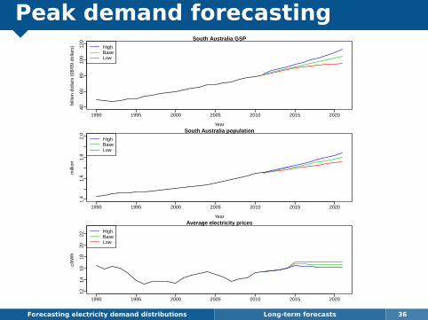
Peak demand forecasting
Forecasting electricity demand distributions Long-term forecasts 36
South Australia GSP
Year
billi
on d
olla
rs (
08/0
9 do
llars
)
1990 1995 2000 2005 2010 2015 2020
4060
8010
012
0
HighBaseLow
South Australia population
Year
mill
ion
1990 1995 2000 2005 2010 2015 2020
1.4
1.6
1.8
2.0
HighBaseLow
Average electricity prices
Year
c/kW
h
1990 1995 2000 2005 2010 2015 2020
1214
1618
2022
HighBaseLow
Major industrial offset demand
Year
MW
1990 1995 2000 2005 2010 2015 2020
010
020
030
040
0
HighBaseLow

Peak demand distribution
Forecasting electricity demand distributions Long-term forecasts 37
PoE (annual interpretation)
Year
PoE
Dem
and
2.0
2.5
3.0
3.5
4.0
98/99 00/01 02/03 04/05 06/07 08/09 10/11
10 %50 %90 %
●
●
●
●
●
●
●●
● ●
●
●
●
●
Peak demand distribution
Forecasting electricity demand distributions Long-term forecasts 37
Annual POE levels
Year
PoE
Dem
and
23
45
6
98/99 00/01 02/03 04/05 06/07 08/09 10/11 12/13 14/15 16/17 18/19 20/21
●●
●
●
●
● ●
● ●
●
●
●●
●
1 % POE5 % POE10 % POE50 % POE90 % POEActual annual maximum

Peak demand forecasting
Forecasting electricity demand distributions Long-term forecasts 38
2.5 3.0 3.5 4.0 4.5 5.0 5.5
0.0
0.5
1.0
1.5
Low
Demand (GW)
Den
sity
2.5 3.0 3.5 4.0 4.5 5.0 5.5
0.0
0.5
1.0
1.5
Base
Demand (GW)
Den
sity
2.5 3.0 3.5 4.0 4.5 5.0 5.5
0.0
0.5
1.0
1.5
High
Demand (GW)
Den
sity
2011/20122012/20132013/20142014/20152015/20162016/20172017/20182018/20192019/20202020/2021

Outline
1 The problem
2 The model
3 Long-term forecasts
4 Short term forecasts
Forecasting electricity demand distributions Short term forecasts 39

Short term forecasts
qt,p = hp(t) + fp(w1,t,w2,t) +
J∑j=1
cjzj,t + nt
Bootstrapping temperatures and residuals is okfor long-term forecasts because short-termdynamics wash out after a few weeks.But short-term forecasts need to take accountof recent temperatures and recent residualsdue to serial correlation.Short-term temperature forecasts are available.Building a separate model for nt is possible, butthere is a simpler approach.
Forecasting electricity demand distributions Short term forecasts 40

Short-term forecasting model
log(yt,p) = hp(t) + fp(w1,t,w2,t) + ap(yt−1) +
J∑j=1
cjzj,t + nt
yt,p denotes per capita demand (minus offset) at time t(measured in half-hourly intervals) during period p,p = 1, . . . ,48;hp(t) models all calendar effects;fp(w1,t,w2,t) models all temperature effects where w1,t isa vector of recent temperatures at location 1 and w2,t isa vector of recent temperatures at location 2;zj,t is a demographic or economic variable at time tnt denotes the model error at time tyt = [yt, yt−1, yt−2, . . . ]ap(yt−1) models effects of recent demands.
Forecasting electricity demand distributions Short term forecasts 41

Short-term forecasting model
ap(yt−1) =n∑
k=1
bk,p(yt−k) +m∑j=1
Bj,p(yt−48j)
+ Qp(y+t ) + Rp(y−t ) + Sp(yt)
where
y+t is maximum of yt values in past 24 hours;
y−t is minimum of yt values in past 24 hours;
yt is average demand in past 7 days
bk,p, Bj,p, Qp, Rp and Sp are estimated usingcubic splines.
Forecasting electricity demand distributions Short term forecasts 42

References
Hyndman, R.J. and Fan, S. (2010) “Densityforecasting for long-term peak electricitydemand”, IEEE Transactions on Power Systems,25(2), 1142–1153.
Fan, S. and Hyndman, R.J. (2012) “Short-termload forecasting based on a semi-parametricadditive model”. IEEE Transactions on PowerSystems, 27(1), 134–141.
Forecasting electricity demand distributions References 43