short‐term electricity demand forecasting with machine
TRANSCRIPT

ii
Short‐Term Electricity Demand Forecasting with
Machine Learning
Ernesto Javier Aguilar Madrid
Panama case study
Project Work presented as the partial requirement for
obtaining a Master's degree in Data Science and Advanced
Analytics

ii
NOVA Information Management School
Instituto Superior de Estatística e Gestão de Informação
Universidade Nova de Lisboa
SHORT‐TERM ELECTRICITY DEMAND FORECASTING WITH MACHINE
LEARNING
Panama case study
by
Ernesto Javier Aguilar Madrid
Project Work presented as the partial requirement for obtaining a Master's degree in Data Science
and Advanced Analytics, specialization in Business Analytics
Advisor: Nuno Miguel da Conceição António
March 2021

iii
ACKNOWLEDGEMENTS
I thank all the people who have been interested in this project's progress. I mainly thank my parents
and sister for their support; to my advisor, professor Nuno Antonio, for accepting this project for his
valuable time and guidance. Also, I want to acknowledge my professors and colleagues who helped
me develop as a person and a professional throughout my career.

iv
ABSTRACT
An accurate short-term load forecasting (STLF) is one of the most critical inputs for power plant units’
planning commitment. STLF reduces the overall planning uncertainty added by the intermittent
production of renewable sources; thus, it helps to minimize the hydro-thermal electricity production
costs in a power grid. Although there is some research in the field and even several research
applications, there is a continual need to improve forecasts. This project proposes a set of machine
learning (ML) models to improve the accuracy of 168 hours forecasts. The developed models employ
features from multiple sources, such as historical load, weather, and holidays. Of the five ML models
developed and tested in various load profile contexts, the Extreme Gradient Boosting Regressor
(XGBoost) algorithm showed the best results, surpassing previous historical weekly predictions based
on neural networks. Additionally, because XGBoost models are based on an ensemble of decision
trees, it facilitated the model’s interpretation, which provided a relevant additional result, the
features’ importance in the forecasting.
KEYWORDS
Short-Term Load Forecasting; Machine Learning; Weekly forecast; Electricity market; Extreme
Gradient Boosting Regressor (XGBoost)

v
INDEX
1. Introduction ................................................................................................................ 10
1.1. Background .......................................................................................................... 10
1.2. Problem and justification .................................................................................... 10
1.3. Objectives ............................................................................................................ 11
2. Literature review ........................................................................................................ 12
2.1. Short-Term Load Forecasting .............................................................................. 12
2.2. Forecasting Methods ........................................................................................... 12
2.2.1. Classical Statistical Time-Series models ....................................................... 12
2.2.2. Machine Learning Regression models .......................................................... 13
2.2.3. Deep Learning models .................................................................................. 16
2.2.4. Combined techniques and other forecasting approaches ........................... 16
3. Methodology .............................................................................................................. 18
3.1. Hardware and Software ...................................................................................... 18
3.2. Data sources, extraction, and transformation .................................................... 18
3.3. Data pre-processing............................................................................................. 19
3.3.1. Missing values and outliers .......................................................................... 19
3.3.2. Feature Engineering ..................................................................................... 19
3.3.3. Feature Selection .......................................................................................... 19
3.3.4. Dataset split into train and test datasets ..................................................... 20
3.4. Modelling ............................................................................................................. 21
3.4.1. Machine Learning candidate models ........................................................... 21
3.4.2. Models training and hyperparameter tuning............................................... 23
3.5. Evaluation metrics ............................................................................................... 25
4. Results and discussion ................................................................................................ 26
4.1. Forecast Results ................................................................................................... 26
4.2. Feature Importance Results ................................................................................ 30
4.3. Hyperparameter Search Results .......................................................................... 31
4.4. Benchmarking ...................................................................................................... 34
5. Conclusions ................................................................................................................. 35
6. Limitations and recommendations for future works ................................................. 36
7. Bibliography ................................................................................................................ 37
8. Appendices ................................................................................................................. 44
8.1. Appendix 1. Data repository ................................................................................ 44

vi
8.2. Appendix 2. Date-time splits ............................................................................... 44
8.3. Appendix 3. Hourly load illustration for each training-testing pair .................... 45
8.3.1. Testing week 1. Week 15, April 2019. Holy week. ....................................... 45
8.3.2. Testing week 2. Week 21, May 2019. .......................................................... 45
8.3.3. Testing week 3. Week 24, June 2019. .......................................................... 46
8.3.4. Testing week 4. Week 29, July 2019. ........................................................... 46
8.3.5. Testing week 5. Week 33, August 2019. ...................................................... 47
8.3.6. Testing week 6. Week 37, September 2019. ................................................ 47
8.3.7. Testing week 7. Week 41, October 2019. .................................................... 48
8.3.8. Testing week 8. Week 44, November 2019. National holidays. .................. 48
8.3.9. Testing week 9. Week 51, December 2019. Christmas. ............................... 49
8.3.10. Testing week 10. Week 1, January 2020. Martyrs Day. ........................ 49
8.3.11. Testing week 11. Week 6, February 2020. ............................................ 50
8.3.12. Testing week 12. Week 10, March 2020. .............................................. 50
8.3.13. Testing week 13. Week 20, May 2020. Quarantine period. .................. 51
8.3.14. Testing week 14. Week 24, Jun 2020. Quarantine period. ................... 51

vii
LIST OF FIGURES
Figure 1. National electricity load vs. Temperature in Panama City. ....................................... 20
Figure 2. Hybrid model structure. ............................................................................................ 22
Figure 3. Sliding window time-based cross-validation. ............................................................ 23
Figure 4. Box-whisker plots for each candidate model and the pre-dispatch load forecast.
(a) MAPE evaluation results;
(b) RMSE evaluation results ............................................................................................. 26
Figure 5. Pre-dispatch and XGB forecast comparison with the real load.
(a) Week 51, 2019 (21st to 27th, Dec 2019);
(b) Week 10, 2020 (7th to 13th, Mar 2019);
(c) Week 24, 2020 (13th to 19th, Jun 2019) ....................................................................... 29
Figure 6. Weekly pre-dispatch vs. ML candidates’ models.
(a) Hourly forecast for Week 15, 2019 (13th to 19th, Apr 2019);
(b) Frequency distribution of error by forecast, for Week 15, Apr 2019 ......................... 30

viii
LIST OF TABLES
Table 1. Variables’ description and units of measure .............................................................. 18
Table 2. Hyperparameter space by model ............................................................................... 24
Table 3. Evaluation metrics ...................................................................................................... 25
Table 4. Errors distribution by model, by metric ..................................................................... 27
Table 5. Evaluation metrics by model, for each testing week, and horizon average .............. 28
Table 6. Average feature importance by ML model expressed in percentage ........................ 31
Table 7. Hyperparameter optimization results for regular days’ models, by testing week .... 32
Table 8. Hyperparameter optimization results for holidays’ models, by testing week ........... 33

ix
LIST OF ABBREVIATIONS AND ACRONYMS
ANN Artificial Neural Networks
ARIMA Autoregressive Integrated Moving Average
CND Centro Nacional de Despacho; National Dispatch Center
DL Deep Learning
KNN K-Nearest Neighbors Regressor
L h Electricity Load in hour h
LMA Lags’ Moving Average
LSTM Long Short-Term Memory
MAPE Mean Absolute Percentage Error
ML Machine Learning
MLR Multiple Linear Regression
MWh Megawatt-hour
Pre-disp. Historical weekly pre-dispatch forecast
RF Random Forest Regressor
RMSE Root Mean Squared Error
RNN Recurrent Neural Networks
STLF Short-Term Load Forecasting
SVR Support Vector Regressor
XGB Extreme Gradient Boosting Regressor (XGBoost)

10
1. INTRODUCTION
The electric power system operation is a continuous work that requires real-time coordination from
the power plants to distribution substations to operate within a secure range and conclusively deliver
the electricity service with quality and without interruptions. Before the real-time operational job
arrives, planning should be done to consider the renewable energy production sources’ behavior, the
power plants and grid maintenance, and weight the hydro-thermal resources, so the electricity
production meets a projected demand. This real-time balance between energy generation and load
should be sustained to avoid damages to the grid (Wood et al., 2013).
A power system operation’s planning time scope can be decomposed into three frames, and each of
these frames focuses on specific tasks (Hossein & Mohammad, 2011): short-term, mid-term, and long-
term. The short-term timeframe goes from 1 day to 1 week, focusing more on the power system’s
operational and security aspects. The mid-term timeframe typically considers several weeks to several
months, focusing more on managing the production resources and avoiding the energy deficits with
the existing power plants. Consequently, the long-term timeframe focuses on years to decades,
intending to define the installation of new power plants or changes on the transmission system. These
criteria can vary from region to region; nevertheless, the concept should remain.
1.1. BACKGROUND
The National Dispatch Center (CND) is in charge of the power system planning and operation in
Panama. According to CND methodologies, the goal of forecasting with an acceptable level of deviation
is to anticipate and supply the demand with minimum costs. Short-term forecasting (following week)
is needed to cover security aspects in the electrical system operation.
As stated in the short-term and mid-term methodologies (CND, 2021b), CND does this forecast
planning every week. For short-term scheduling, CND uses an hourly basis optimization software (PSR
NCP, 2021). This optimization tool solves the weekly minimal dispatch cost, and it requires data about
the load forecast, the power plants, and the power grid on an hourly basis. CND is currently using the
Nostradamus tool by HITACHI ABB (HITACHI-ABB, 2021) to forecast the hourly load and feed the short-
term optimization tool to plan the following week’s hourly dispatch (CND-sitr, 2020).
1.2. PROBLEM AND JUSTIFICATION
This work project focuses mainly on predicting the short-term electricity load: this forecasting problem
is known in the research field as short-term load forecasting (STLF), particularly, the STLF problem for
the Panama power system, in which the forecasting horizon is one week, with hourly steps, which is a
total of 168 hours.
As introduced previously, an accurate load forecasting is a critical input for planning. The STLF will help
reduce the planning uncertainty added by the intermittent electricity production from renewable
sources. Afterwards, it will determine the optimum opportunity costs for hydroelectrical power plants
with reservoirs. Consequently, an efficient thermal power plant dispatch can be achieved by
minimizing the unit commitment production-transmission costs for the power system (Aguilar Madrid
& Valdés Bosquez, 2017; Morales-España et al., 2013). Ultimately, the operational costs associated
with dispatching the best set of power plants in real-time dispatch will also be reduced.

11
Because the electricity consumption patterns evolve, and new machine learning (ML) approaches are
emerging, the motivation to explore and update the forecasting tools arises by seeking to implement
the most efficient and robust methods to minimize errors.
1.3. OBJECTIVES
The current project aims to develop better STLF models. The models will be evaluated with the
Nostradamus’ historical weekly forecasts for Panama’s power grid to benchmark the models’
performance against the Nostradamus forecasts in an effort to show that it is possible to improve the
168 hours STLF. This project’s dataset includes historical load, a vast set of weather variables, holidays,
and historical load weekly forecast features to compare the proposed ML approaches and achieve the
above-declared objectives.
It is essential to remark the exclusion of exports cross-border demand from this forecast since this load
does not belong to Panama. Also, because this load is constrained for grid security aspects and
planned, for instance, it does not obey natural consumption behavior.

12
2. LITERATURE REVIEW
This section presents a review of the literature related to this project, taking as main references studies
and books that expose methodologies and algorithms to forecast in the short-term, focusing on
electricity load forecasting.
2.1. SHORT-TERM LOAD FORECASTING
The short-term electricity load forecasting is implemented to solve a wide range of needs, providing a
wide range of applications, and for instance, there is a vast research field. The most evident difference
between research is the load scale, from a single transformer (Becirovic & Cosovic, 2016), to buildings
(Cao et al., 2020), to cities (Fernandes et al., 2011), regions (Sarmiento et al., 2008) and even countries
(Adeoye & Spataru, 2019). The second most crucial distinction among the research field is the
forecasting horizon. Varying from very short-term applications, like forecasting the next 900 seconds
for machine tools (Dietrich et al., 2020), moving to a few hours (Lebotsa et al., 2018), forecasting for
the day-ahead, which is the most common (Zhu et al., 2021), and 48 hours ahead (Ferreira et al., 2013),
to weekly forecasts (Zou et al., 2019). The forecasting granularity also varies among the research field.
Having granularities from 15 minutes, 30 minutes, but most of the approaches consider hourly
granularity forecasting. Despite the variety of the forecasting applications, this literature review will
focus on covering implemented methodologies, chosen variables, algorithms, and evaluation criteria,
since the forecast success will heavily depend on the decisions made through these development
stages.
2.2. FORECASTING METHODS
A wide variety of methodologies and algorithms have been implemented to address STLF. From the
most straightforward Persistence method, proposed by (Dutta et al., 2017), which follows the basic
rule of “today equals tomorrow”. To the most recent deep learning algorithms as exposed in the
review article by (Paterakis et al., 2017), which compares traditional machine learning approaches with
deep learning methods on the electricity forecasting field, as well as the most trending algorithms
Scopus-indexed publications from the year 2005 to 2015.
2.2.1. Classical Statistical Time-Series models
Time series analysis is considered one of the most widely discussed forecasting methodologies in which
the Box-Jenkins and Holt-Winters procedures are extensively used. For example (Barakat & Al-Qasem,
1998) used those methods to forecast the weekly load for Riyadh Power System in Saudi Arabia,
concluding that these approaches give insights to decompose the electric load forecast.
The autoregressive integrated moving average model (ARIMA) is a classical time series model which
has been widely utilized in various forecasting tasks. (Amjady, 2001) proposed a modified ARIMA, to
forecast the next 24 hours in Iran. This modified ARIMA combines the estimation with temperature
and load data, producing an enhancement to the traditional ARIMA model. The ARIMA model by itself
does not significantly improve the forecast accuracy and is computationally more expensive,
demonstrating the need to complement these models with external inputs to enhance the results.

13
Overall, in most recent research, these models are less used for electricity STLF, since machine learning
methods provide better results, as demonstrated by (Al-Musaylh et al., 2018), (Amin & Hoque, 2019),
and more recently by (X. Liu et al., 2020). Particularly, in this last cited study, the authors compare the
performance of six classical data-driven regression models and two deep learning models to deliver a
day-ahead forecast for Jiangsu province, China, concluding that the ARIMA model had several
limitations to solve the STLF problem.
Based on researchers’ results and conclusions, it is noticeable that the ARIMA as a time series method
has several limitations to solve the STLF problem. Firstly, because it can only consider time-series data
to forecast based on the electrical load. Second, the determination of the model order is either
computationally expensive or empirical. Lastly, to make residuals uncorrelated, several trials are
required. At the same time, autocorrelation function (ACF) and partial autocorrelation function (PACF)
graphs need to be iteratively checked to tune the model.
2.2.2. Machine Learning Regression models
From the wide range of machine learning (ML) models, regression models are suitable for the
forecasting task. The developed state of art for STLF showed that the most used machine learning
models are Multiple Linear Regression (MLR), Artificial Neural Networks (ANN), Support Vector
Machine Regression (SVR), Decision Tree Regression (DT), Random Forest Regressor (RF), Gradient
Boosted Regression Trees (GB) and Extreme Gradient Boosting Regressor (XGB). In some studies,
models like K-Nearest Neighbors Regressor (KNN), Ridge regression, Lasso regression and Gaussian
Process are used as a baseline to compare the accuracy of other models.
Multiple Linear Regression (MLR)
In contrast with the classical statistical time-series models, ML models can handle more valuable
factors, such as weather conditions, to improve the STLF accuracy. Multiple linear regression (MLR)
has been widely used for STLF, for example (Chapagain & Kittipiyakul, 2018) used it to forecast the
hourly weekly load in Thailand, obtaining an average mean absolute percentage error (MAPE) of 7.71%
for 250 testing weeks and pointing out that temperature is a primary factor to predict load. Similarly,
(Adeoye & Spataru, 2019) utilized MLR to forecast electricity consumption 24 h ahead for 14 west-
African countries, considering weather variables like temperature, humidity, and daylight hours. (Do
et al., 2016) propose to use estimated as 24 independent MLR models, one for each hour of the day,
to forecast the day-ahead demand in Germany. They used temperature, industrial production, hours
of daylight and dummies for days of the week and month of the year as explanatory variables. They
conclude that despite using a simple MLR, forecasts hourly electricity demand more precisely than a
single MLR for the 24 hours, obtaining a yearly MAPE of 2.3%. Researchers that have implemented
MLR agreed on the fast training and interpretability this model offers, although it shows poor
performance for irregular load profiles.
Artificial Neural Network (ANN)
The neural network's approach is widely used for STLF during the last decades due to the algorithm
flexibility. For example (F. Liu et al., 2006) proposed ANN with Levenberg-Marquardt training
algorithm to forecast hourly, daily and weekly load in Ontario, Canada, presenting good results but
without comparing with other algorithms. Furthermore, (Becirovic & Cosovic, 2016) forecasted a single

14
transformer hourly load, using quarter-hour load records and weather data with hourly records,
obtaining a MAPE performance below 1% with ANN for summer and winter seasons.
In a more recent study (Li, 2020) applies STLF for urban smart grid system in Australia, commenting
that ANN has good generalization ability for the task. However, this approach still has many
disadvantages as quickly falling into a local optimum, overfitting, and exhibiting a relatively low
convergence rate. To overcome these obstacles, he implemented a multi-objective optimization
approach to optimize the weight and threshold of the neural network to simultaneously enhance
forecasting accuracy and its stability, which is a complex solution compared with others along with
state of the art. Nevertheless, the complexity of forecasting smart grids loads with increasing
renewable energy sources is challenging and deserves complex solutions to obtain good results.
Support Vector Regression (SVR)
The SVR model is the regression version of the Support Vector Machine algorithm (SVM) which was
initially designed for classification problems. Nevertheless, it is a popular model for STLF, mainly with
a linear kernel, due to the linearity between the inputs and the forecast, as concluded by (X. Liu et al.,
2020); who obtained a MAPE under 2.6 % for the day-ahead prediction of Jiangsu, performing better
than MLR and multivariate adaptive regression splines.
(Ferreira et al., 2013) proposed to forecast the 48 hours Portuguese electricity consumption by using
SVR as a better alternative after submitting the use of ANN for the same task (Ferreira et al., 2010).
The main reason for preferring SVR was the efficiency of the hyperparameter tunning on the daily on-
line forecast. The SVR achieve a MAPE between 1.9 % and 3.1 % for the first-day forecast and between
3.1 % and 4 % for the second-day.
A variant of SVR is compared against ANN by (Omidi et al., 2015) to forecast the south-Iranian day-
ahead hourly load. They proposed the nu-SVR, which improves upon SVR by changing the algorithm
optimization problem and automatically allowing the epsilon tube width to adapt to data. They
evaluate both models for each season; the average MAPE was 2.95 % for nu-SVR and 3.24 % for ANN.
(Y. Cai et al., 2011) implemented genetic algorithms to search the optimal values of SVR parameters to
predict the power load specifically for holidays in Hebei province of China. Holidays STLF is challenging
due to the limited historical records and the irregular people’s electricity consumption during these
periods. Their results achieved a mean relative error of 3.22% for a regular day and 3.92%.
Random Forest Regressor (RF)
Random Forest is part of the ensemble learning models; ensemble technique combines a set of
independent learners to improve the forecasting ability of the overall model. (Pinto et al., 2021) took
advantage of this principle to forecast the day-ahead hourly consumption in office buildings. They used
many ensemble algorithms, with RF being one of them, including environmental variables such as
temperature and humidity and lagged load records to improve the results. Finally, they obtained a
6.11% MAPE for RF.
Similarly, (Hadri et al., 2019) submitted a comparative study between many models to forecast smart
buildings’ electricity load. ARIMA, Seasonal ARIMA (SARIMA), RF, and extreme gradient boosting (XGB)
were on this set of models. Their experiments demonstrated that RF showed decent results, but XGB

15
outperformed the other methods, concluding that XGB gives better accuracy and better performance
in terms of execution time. The study from (J. Cai et al., 2020) compares RF solely with XGB to forecast
the next 24 hours load and also conclude that XGB, as an emerging ensemble learning algorithm, can
achieve higher prediction accuracy. Producing a RMSE of 3.31 for RF and 2.01 for XGB.
(Zhang et al., 2019) presented an interesting case study to forecast the day-ahead load from Southern
California, with the difference that the increase in behind-the-meter residential PV generation has
made it more difficult to predict the region load. Nonetheless, they elaborated a detailed variable
selection along 45 variables, in which temperature, holiday, month, and previous week load were
essential features to train the models. This study compares MLR, RF and Gradient Boosting. Their
results showed that all three models were more accurate when the electrical load was low. In contrast,
models had larger errors during peak hours and the summer season, when the electrical load was
higher. The Gradient Boosting model was generally superior to the MLR and RF models.
Extreme Gradient Boosting (XGB)
As mentioned by the XGBoost documentation (XGB Developers, 2021): “XGBoost is an optimized
distributed gradient boosting library designed to be highly efficient, flexible and portable. It
implements ML algorithms under the Gradient Boosting framework”. For instance, it is an enhanced
version of Gradient Boosting.
Most recent research, like the one presented by (Suo et al., 2019) suggests the use of XGB. In this work,
they use weather variables and historical load to forecast the hourly weekly load of a power plant.
Remarking on the complexity of XGB hyperparameter phase and suggesting the fireworks algorithm to
obtain the global minimum on the hyperparameter space, and for instance, getting a more accurate
load forecast.
As mentioned earlier, forecasting holidays is challenging. Though (Zhu et al., 2021) argue that there
are many matured predictive methods for STLF, such as SVR, ANN, and deep learning (DL). However,
those methods have some issues: SVR is not robust to outliers, ANN has the weakness of setting the
correct number of hidden layers or can be easily trapped into a local minimum, and DL approaches
require massive high-dimensional datasets for good performance. XGB lacks these issues and
outperforms the others for solving STLF. Their results are based on averaging the daily profile curves
for similar holidays plus the use of XGB, where this averaging plus XGB outperforms RF, SVR, ANN, and
even the sole-use XGB.
Despite the good XGB performance, some authors recommend training the model based on similar
days to enhance the forecast (Liao et al., 2019; Y. Liu et al., 2019). A comparison between a traditional
XGB and the similar days’ XGB is demonstrated by (Liao et al., 2019). The similar days’ approach
showed a noticeable improvement, emphasizing that the accurate selection of similar days will directly
affect the STLF.
Similarly, (Liao et al., 2019) compare the results of the traditional XGB, a Long Short-Term Memory
(LSTM), and an XGB based on similar days. The similar days’ pre-processing phase is based on a cluster
analysis that subsequently will feed the XGB model. The MAPE of the proposed XGBoost model was
8.8 % against 12 % of the traditional XGB and 13 % of the LSTM.

16
2.2.3. Deep Learning models
Long Short-Term Memory (LSTM)
From all neural network’s approaches, Recurrent Neural Networks (RNN) are taking an important place
in the STLF field, especially LSTM, because contrary to standard feedforward neural networks, LSTM
has feedback connections. Which is beneficial to deal with time-series forecasting applications. Many
authors are recently using it because of its remarkable results in time series learning tasks like the
hourly weather forecast, and solar irradiation (Zou et al., 2019). (Yan et al., 2019) attempt to forecast
the next 24 hours load from a smart grid. They compared the LSTM results with a back-propagation
ANN and SVR, demonstrating that LSTM can offer a MAPE of 1.9 % against 3.3 % from ANN and 4.8 %
of SVR.
The work published by (Abbasimehr et al., 2020) addresses the STLF for a furniture company with a
method based on a multilayer LSTM and compare it to other models like ARIMA, exponential
smoothing, k-nearest neighbors regressor, and ANN. Moreover, their results showed that LSTM
performed better in both RMSE and MAPE, followed by SVM and ANN.
A noteworthy contribution is published by (Atef & Eltawil, 2020), using Switzerland load and
temperature data. According to these researchers, deep learning methods has a superior performance
in electricity STLF, however, “the potential of using these methods has not yet been fully exploited in
terms of the hidden layer structures.” For this reason, they evaluate deep-stacked LSTM with multiple
layers for both Unidirectional LSTM (Uni-LSTM), Bidirectional LSTM (Bi-LSTM), and SVR as a baseline
model. Their results showed that Bi-LSTM MAPE was 0.22% against MAPE above 2% for Uni-LSTM and
SVR.
2.2.4. Combined techniques and other forecasting approaches
Because XGB provides the feature importance property, the authors of Reference (Zheng et al., 2017)
proposed a hybrid algorithm to classify similar days with K-means clustering fed by XGB feature
importance results. Once the classification is done, an empirical mode method is used to decompose
similar days’ data into several intrinsic mode functions to train separated long short-term memory
(LSTM) models, and finally, a time-series reconstruction from individual LSTM model predictions. This
hybrid model using LSTM performed better for STLF over 24 and 168 hours horizons, after comparing
with ARIMA, SVR, and back-propagation neural network using the same similar day approach as initial
input.
(Xue et al., 2019) proposed a multi-step-ahead forecasting methodology using XGB and SVR to forecast
hourly heat load, where “direct” and “recursive” forecasting strategies are compared. The direct
method involves an independent model to predict each period on the forecasting horizon, while the
“recursive” method considers a unique model that iterates one step at a time over the forecasting
horizon, using the previous predicted steps as an input variable for the following forecasting step.
Performance is the main disadvantage of the direct strategy because it needs to train as many models
as desired periods to forecasts. The recursive strategy is sensitive to prediction errors, meaning that
prediction errors will propagate along the forecasting horizon.
A study to forecast the 10-day streamflow for a hydroelectric dam used a decomposition-based
methodology to compare XGB and SVR (Yu et al., 2020). In this study, the streamflow time-series were

17
decomposed into seven contiguous frequency components using the Fourier Transform. Then, each
component was forecasted independently by the SVR or XGB. The study results showed that SVR
outperformed XGB in terms of evaluation criteria through the Fourier decomposition methodology.
Another solution joining ANN with ensemble approaches is presented by (Khwaja et al., 2020), where
the authors seek to improve ANN generalization ability using bagging-boosting. When training
ensembles of ANNs in parallel, each ensemble uses a bootstrapped sample of the training data and
consists of training the ANNs sequentially, and this method reduces the STLF error but increases the
computational time because of the several training procedures. Alternatively, to training several ANN
sequentially, (Singh & Dwivedi, 2018) propose an evolutionary novel optimization procedure for tuning
an ANN. For instance, avoiding the issues related to ANN tuning like overfitting and selecting the best
ANN architecture. Their results achieved a 4.86% MAPE. Based on the results from (F. Liu et al., 2006;
Zheng et al., 2017), ANN for STLF can outperform other forecasting methods if a robust
hyperparameter optimization is performed to avoid the issues related to ANN tuning.
The hybridization of the successive geometric transformations model (SGTM) neural-like structure is
another promising approach for STLF, as used by (Vitynskyi et al., 2018) to predict Libya’s solar
radiation. This approach demonstrated a higher accuracy than MLR, SVR, RF, and multilayer
perceptron neural network, besides having a faster training time due to the non-iterative training
procedure.

18
3. METHODOLOGY
3.1. HARDWARE AND SOFTWARE
This project was developed on a computer with an i5-9300H processor and 8 Gigabytes of RAM. Colab
(Google, 2020) hosted Jupyter notebooks service, which provides two vCPU and 12 Gigabytes of RAM
per session, and JupyterLab notebook instances from Google Cloud Platform (GCP, 2021) for more
extensive executions, selecting the 16 vCPU and 64 Gigabytes of RAM configuration. All the
experiments were developed with Python (Rossum et al., 2009).
3.2. DATA SOURCES, EXTRACTION, AND TRANSFORMATION
All data sources to develop this project are publicly available; the data will consider hourly records
from January 2015 until June 2020 and are the following:
1. Historical electricity load from Panama, available on daily post-dispatch reports (CND, 2021c), and
historical weekly forecasts available on weekly pre-dispatch reports (CND, 2021e).
2. Calendar information related to holidays, and school period, provided by Panama’s Ministry of
Education trough Official Gazette (Gaceta, 2020) and holidays websites (When On Earth?, 2021).
3. Weather variables, such as temperature, relative humidity, precipitation, and wind speed from
three main cities in Panama, are gathered from EarthData satellite data (GES DISC, 2015).
The load datasets are available in Excel files on a daily and weekly basis, with hourly granularity.
Holidays and school periods data is sparse, along with websites and PDF files. These periods are
represented with binary variables, and date ranges are manually inputted into Excel files. Both Excel
datasets are imported and converted into data frames (McKinney & Team, 2020). Weather data is
available on daily NetCDF files, which can be treated with netCDF (Nadh, 2021) and xarray (Hoyer &
Hamman, 2017) to select the desired variables and subsequently convert these datasets into data
frames. Once all datasets were in the same data frame format, they were merged on date-time index.
Finally, the result of these steps is: a time-series with the historical forecast along with its date-time
timestamp as the index, and a data frame with the same timestamp index and 16 columns, one for
each of the following features shown in Table 1. Both objects have 48,048 records. Where sub-index c
stands for city, meaning that weather variables are available for David, Santiago, and Panama City.
Variable Description Unit of measure
National load National electricity load, excluding exports MWh
Holiday Holiday binary indicator -
Holiday ID Holiday identification number -
School School period binary indicator -
Temp. 2mc 2 meters air temperature ºC
Hum. 2mc 2 meters specific humidity %
Wind 2mc 2 meters wind speed m/s
Precipitationc Total precipitable liquid water l/m2
Load Forecast Historical national load forecast, excluding exports MWh
Table 1. Variables’ description and units of measure.

19
3.3. DATA PRE-PROCESSING
3.3.1. Missing values and outliers
There are no missing values on the datasets, and an initial outlier’s revision was made by normalizing
each variable. Only a few low values on the load were detected due to hourly blackouts and damages
in the power grid, but all records were kept.
3.3.2. Feature Engineering
The set of variables used to train the ML models, also called features, are treated in this section. New
variables related to the date-time index are created to feed the ML models with this extra information
about time, with this being one of the most critical steps for STLF (X. Liu et al., 2020; Zhang et al., 2019).
The new features added to the datasets are year, month number, day of the month, week of the year,
day of the week, the hour of the day, the hour of the week, weekend indicator. All being integer
variables, except for the binary weekend indicator. It is essential to clarify that Saturday is considered
the first day of the week. For instance, the first week of each year is the first complete week starting
on Saturday, and this is respected to keep the CND reports calendar structure for further comparisons.
Load weekly lags and load weekly moving average features were new calculated features that help to
capture the most recent changes of load (Pinto et al., 2021), keeping the hourly granularity. These
were calculated from the second preceding week until the fourth week, adding two more features to
the current dataset.
Given an hour 𝒉, to forecast the load 𝑳 at this hour 𝑳𝒉, the load’s lags can be denoted as 𝑳𝒉−𝒊, where
𝒊 remains in the hourly granularity. Following this notation, the included lag features are: 𝑳𝒉−𝟏𝟔𝟖,
𝑳𝒉−𝟑𝟑𝟔, 𝑳𝒉−𝟓𝟎𝟒 and 𝑳𝒉−𝟔𝟕𝟐 which corresponds to the previous week, the second last, third last and
fourth last week’s load. The lags’ moving averages (LMA) are calculated from the weekly lags following
equation (1). The independent variable 𝒎 represents the earliest week to consider, and 𝒏 stands for
the latest week to consider in the moving average. Following equation (1), the considered LMA were
𝑳𝑴𝑨𝒉(𝟏, 𝟑) and 𝑳𝑴𝑨𝒉(𝟏, 𝟒).
𝑳𝑴𝑨𝒉(𝒎, 𝒏) =∑ 𝑳𝒉−𝟏𝟔𝟖𝒎+𝑳𝒉−𝟏𝟔𝟖(𝒎+𝟏)+⋯ + 𝑳𝒉−𝟏𝟔𝟖(𝒏−𝟏)+𝑳𝒉−𝟏𝟔𝟖𝒏
𝒏𝒎
𝒏−𝒎+𝟏 ; 𝑤ℎ𝑒𝑟𝑒 𝒎 ≥ 𝟏 ∧ 𝒏 > 𝒎 (1)
3.3.3. Feature Selection
The decision of which variables should be used to train the ML models is critical to obtain good results.
This process, known as feature selection, also reduces computation time, decreases data storage
requirements, simplifies models, evades the curse of dimensionality, and enhances generalization,
avoiding overfitting (Eseye et al., 2019). For these reasons, several feature selection techniques were
performed along with the STLF state-of-the-art (Becirovic & Cosovic, 2016; X. Liu et al., 2020); and the
problem understanding to select essential features. The explored Feature Selection techniques were:
feature variance, correlation with the target, redundancy among regressors (Han et al., 2011), and
feature importance according to the default models multiple linear regression, decision tree regressor,
random forest regressor, and extreme gradient boosting regressor.

20
After having 28 regressors and a defined target, the feature selection analysis showed that 10
regressors would significantly contribute to forecast. Consequently, the best regressors are:
▪ 𝐿𝒉−𝟑𝟑𝟔
▪ 𝐿𝒉−𝟓𝟎𝟒
▪ 𝐿𝒉−𝟔𝟕𝟐
▪ 𝐿𝑀𝐴𝒉(𝟏, 𝟒)
▪ 𝑑𝑎𝑦_𝑜𝑓_𝑡ℎ𝑒_𝑤𝑒𝑒𝑘𝒉
▪ 𝑤𝑒𝑒𝑘𝑒𝑛𝑑_𝑖𝑛𝑑𝑖𝑐𝑎𝑡𝑜𝑟𝒉
▪ ℎ𝑜𝑙𝑖𝑑𝑎𝑦_𝑖𝑛𝑑𝑖𝑐𝑎𝑡𝑜𝑟𝒉
▪ ℎ𝑜𝑙𝑖𝑑𝑎𝑦_𝐼𝐷𝒉
▪ ℎ𝑜𝑢𝑟_𝑜𝑓_𝑡ℎ𝑒_𝑑𝑎𝑦𝒉
▪ 𝑡𝑒𝑚𝑝𝑒𝑟𝑎𝑡𝑢𝑟𝑒_2𝑚_𝑖𝑛_𝑃𝑎𝑛𝑎𝑚𝑎_𝑐𝑖𝑡𝑦𝒉
The temperature was an essential weather variable due to its positive relationship with electricity load
(Boya, 2019), as illustrated in Figure 1. This figure shows the typical load range, from 800 to 1600 MWh,
and a temperature range between 23 and 33 ºC. The dashed line identifies the linear equation (2):
𝑳𝒉 = 4.8 ∙ 𝑡𝑒𝑚𝑝𝑒𝑟𝑎𝑡𝑢𝑟𝑒_2𝑚_𝑖𝑛_𝑃𝑎𝑛𝑎𝑚𝑎_𝑐𝑖𝑡𝑦𝒉 − 867.5 (2)
Which indicates that 1 °C increase in temperature represents a 74.8 MWh electricity load increase.
Figure 1. National electricity load vs. Temperature in Panama City.
3.3.4. Dataset split into train and test datasets
Before splitting the data into training and test datasets, the hourly records at the beginning and the
end of the horizon are dropped if they do not belong to a complete 168 hours weekly block for
consistency on training, validation, and testing. After this, 283 complete weeks are available with
hourly records. The dataset is split into train and test, keeping the chronological records. Records are
sorted by date-time index, always leaving the last week for testing and the remaining older data for
training. Based on this logic, there are 14 pairs of train-test datasets selected. Twelve pairs, having a
testing week for each month of the last year of records before the 2020 quarantine started due to the
COVID-19 pandemic, and two more after the quarantine began. To note, the official lockdown in
Panama started on Wednesday, 25 March of 2020, which corresponds to week 12—2020 (La Estrella
de Panamá, 2021). More details about the 14 train-test pairs are available in appendices 2 and 3.
0
400
800
1200
1600
2000
22 24 26 28 30 32 34 36
Elec
tric
ity
load
(M
Wh
)
Temperature in Panama city (ºC)

21
These criteria test the models under regular and irregular conditions since the quarantine period
presented a lower demand with atypical hourly profiles. The selected testing weeks also included
typical days and holidays to test the models on different conditions throughout the year.
As mentioned in the background section, the planning process is weekly done, typically starting every
Wednesday to forecast the week starting on Saturday as the first day of the weekly planning horizon.
So, the available records for forecasting usually are updated every Tuesday at midnight, then executed
on Wednesdays for the planning 168 hours horizon that starts every Saturday and finishes on each
Friday. For this reason, the forecast should consider at least a gap of 72 hours of unseen data before
the first period to predict.
3.4. MODELLING
3.4.1. Machine Learning candidate models
Studies have shown that many decision-makers exhibit an inherent distrust of automated predictive
models, even if they are proven to be more accurate than human forecasters (Dietvorst et al., 2015).
One way to overcome “algorithm aversion” is to provide them with interpretability (Bertsimas et al.,
2019). For these reasons, the current project explores a set of candidate ML models that have been
proven as forecasters within the STLF state-of-the-art, but also models that can offer a certain level of
interpretability.
The candidate ML models considered in this project are Multiple Linear Regression (MLR), k-nearest
neighbors regressor (KNN), epsilon-support vector regression (SVR), random forest regressor (RF), and
extreme gradient boosting regressor (XGB). All these estimators were executed using a pipeline with a
default Min–Max scaler as the first step. These ML models, the pipeline structure, and the scalers were
from sci-kit learn (Pedregosa et al., 2011), except for XGB (XGB Developers, 2021).
MLR uses two or more independent variables to predict a dependent variable by fitting a linear
equation. This method’s assumptions are that: the dependent variable and the residuals are normally
distributed, there are linear relationships between the dependent and independent variables, and no
collinearity should exist between regressors. Since MLR can include many independent variables, it can
provide an understanding of the relationships (Zhang et al., 2019), but it presents the disadvantage of
being sensitive to outliers.
KNN is not typical for STLF. Nevertheless, their results can be interpreted, and some researchers used
it as a baseline model (Johannesen et al., 2019). The KNN method searches for the k most similar
instances; when the k most similar samples are found, the target is obtained by local interpolation of
the targets associated with the k found instances (Abbasimehr et al., 2020). The main disadvantage of
this method is that it tends to overfit, and it has few hyperparameters to change this situation.
SVR is a regression version of the Support Vector Machine (SVM) which was initially designed for
classification problems (Vinet & Zhedanov, 2011). In contrast to ordinary least squares of MLR, the
objective function of SVR is to minimize the L2-norm of the coefficient vector, not the squared error.
The error term is then constrained by a specified margin ε (epsilon). SVR is frequently used for STLF
with the linear (X. Liu et al., 2020) or radial basis function (RBF) kernel (Cao et al., 2020), identifying
load patterns better than other linear models (Amin & Hoque, 2019).
22
RF is an ensemble learning method with generalization ability. It fits many decision trees on various
sub-samples of the dataset and uses averaging to improve the forecast and avoid overfitting. For these
reasons, it seems suitable for STLF, but the few researchers that consider this model have
demonstrated a weak performance on their results (Pinto et al., 2021).
XGB is another ensemble ML algorithm based on gradient boosting library, but enhanced and designed
to be highly efficient, flexible, and portable (XGB Developers, 2021). Providing a forward stage-wise
additive model that fits regression trees on many stages while the regression loss function is
minimized. Due to its recent development, XGB is not a matured STLF method, though, researchers
are starting to use it, showing outstanding performances against traditional methods (J. Cai et al., 2020;
Hadri et al., 2019).
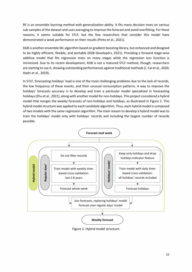
In STLF, forecasting holidays’ load is one of the most challenging problems due to the lack of records,
the low frequency of these events, and their unusual consumption patterns. A way to improve the
holidays’ forecasts accuracy is to develop and train a particular model specialized in forecasting
holidays (Zhu et al., 2021), along with another model for non-holidays. This project considered a hybrid
model that merges the weekly forecasts of non-holidays and holidays, as illustrated in Figure 2. This
hybrid model structure was applied to each candidate algorithm. Thus, each hybrid model is composed
of two models with the same regression algorithm. The main reason to develop a hybrid model was to
train the holidays’ model only with holidays’ records and including the largest number of records
possible.
Forecast next week
Re
gula
r d
ays’
Ho
lida
ys’ m
od
el
Weekly forecast
Do not filter records
Train model with weekly time-
based cross-validation:
last 2.8 years
Forecast whole week
Keep only holidays and drop
holidays indicator feature
Train model with daily time-
based cross-validation:
all holidays’ records included
Forecast holidays
Hyb
rid
mo
de
l
Join forecasts, replacing holidays’ model
forecast over regular days' model
forecast.
Figure 2. Hybrid model structure.

23
3.4.2. Models training and hyperparameter tuning
Once the training and testing weeks pairs were defined, models were trained with the earliest train-
test pair, following the forward sliding window approach (Sugiartawan & Hartati, 2019) for time-based
cross-validation (Herman-Saffar, 2021). The idea for time-based cross-validation is to iteratively split
the training set into two folds at each step, always keeping the validation set ahead of the training set.
This process of defining folds, training the model, predicting the validation fold, and evaluating the
model performance while changing hyperparameters and moving the training/validation sets further
into the future is illustrated in Figure 3.
Figure 3. Sliding window time-based cross-validation.
The regular days’ model’s sliding window characteristics are 149 weeks (2.8 years) for
training/validation. Within those, 64 are validation weeks, excluding the last 72 hours from each
validation fold to comply with the three-day unknown gap when forecasting the weekly demand on
real conditions; finally, the forward step on the training/validation process is one week (168 hours).
For the holidays’ model, only holidays records are kept, and the sliding window considers all holidays
records available since the year 2015 (as shown in Figure 2). The forecasting horizon for the holidays’
model is 24 hours; for instance, the sliding window process also considers forecasting a holiday during
the training process.
The hyperparameter tuning was performed with Optuna optimization framework (Akiba et al., 2019),
keeping the sliding window attributes. The models’ tuning process consists of maximizing the “negative
mean root squared error” (-RMSE) while sampling the defined hyperparameter space with the Tree-
structured Parzen Estimator (TPE) algorithm (Bergstra et al., 2011). The optimization studies were
constrained to 30 trials, which implies that 30 different hyperparameter combinations are explored in
the training process. On each trial, for each parameter, TPE fits one Gaussian Mixture Model (GMM)
𝒍(𝒙) to the set of parameter values associated with the best objective values, and another GMM 𝒈(𝒙)
to the remaining parameter values (Optuna, 2018a). Then TPE chooses the parameter value 𝒙 that
maximizes the ratio 𝒍(𝒙)/𝒈(𝒙).
It is valuable to mention that as a first trial to address this STLF task, all candidate’s models were trained
with a two-step randomized and grid-search cross-validation approach as suggested by (Dietrich et al.,
2020), but it resulted computationally too expensive. To reduce the computational work and execution
time, but without losing quality on results, Optuna hyperparameter optimization was chosen; aiming
to simulate the models' updates along the time by training each candidate model before forecasting
each testing week.

24
This hyperparameter tuning was performed individually for both models inside the Hybrid mode: the
regular’s days model and the holidays’ model. The hyperparameter optimization was performed for
each testing week, aiming to predict each testing week with updated models along the time. The
explored hyperparameter space for each algorithm is shown in Table 2. The absent parameters were
considered with their default value, and the hyperparameter spaces are expressed in terms of the trial
method from Optuna, which describes more precisely the explored distributions and ranges of values
for each parameter (Optuna, 2018b).
Model Hyperparameter Hyperparameter space
KNN
n_neighbors suggest_int('n_neighbors', 3, 50, 2)
weights suggest_categorical('weights', ['uniform', 'distance'])
metric suggest_categorical('metric', ['minkowski', 'euclidean', 'manhattan'])
leaf_size suggest_int('leaf_size', 1, 50, 5)
SVR
kernel suggest_categorical('kernel', ['linear', 'rbf'])
epsilon suggest_loguniform('epsilon', 0.0001, 10)
C suggest_loguniform('C', 0.001, 3000)
tol trial.suggest_uniform('tol', 1×10⁻⁵, 1×10⁻²)
gamma suggest_categorical('gamma', ['scale', 'auto'])
RF
criterion mse
n_estimators suggest_int('n_estimators', 40, 200, 20)
max_samples suggest_discrete_uniform('max_samples', 0.6, 0.9, 0.05)
max_depth suggest_int('max_depth', 7, 21, 3)
ccp_alpha suggest_loguniform('ccp_alpha', 1×10⁻⁶, 1×10⁻³)
random_state 123
XGB
eval_metric rmse
n_estimators suggest_int('n_estimators', 300, 500, 50)
max_depth suggest_int('max_depth', 3, 7)
subsample suggest_discrete_uniform('subsample', 0.6, 0.9, 0.05)
colsample_bytree suggest_discrete_uniform('colsample_bytree', 0.6, 0.9, 0.05)
colsample_bylevel suggest_discrete_uniform('colsample_bylevel', 0.6, 0.9, 0.1)
colsample_bynode suggest_discrete_uniform('colsample_bynode', 0.6, 0.9, 0.1)
learning_rate suggest_loguniform('learning_rate',0.0001, 0.1)
min_child_weight suggest_int('min_child_weight', 1, 7, 2)
gamma suggest_loguniform('gamma', 0.00001, 2)
lambda suggest_loguniform('reg_lambda', 1, 5)
alpha suggest_loguniform('reg_alpha', 0.00001, 2)
random_state 123
Table 2. Hyperparameter space by model.

25
3.5. EVALUATION METRICS
This project addresses many evaluation metrics to systematically evaluate the ML models’
performance, including the traditional metrics for ML forecasting, as well as other specific metrics for
STLF. These evaluation metrics and their formulation are listed in Table 3. Where 𝑨 is a weekly set of
actual hourly load values, 𝑭 is a weekly set of forecasted hourly values, and subindex 𝒉 stands for a
specific hour. For this project, all testing sets were whole weeks with 168 hours, so 𝒏 is equal to 168.
Metric Definition Equation Unit
MAPE Mean Absolute Percentage Error 𝑀𝐴𝑃𝐸 = 1
𝑛∑ |
𝐴ℎ − 𝐹ℎ
𝐴ℎ
|𝑛
ℎ=1× 100% %
RMSE Root Mean Square Error 𝑅𝑀𝑆𝐸 = √1
𝑛∑ (𝐴ℎ − 𝐹ℎ)2
𝑛
ℎ=1 MWh
Peak Peak Load Absolute Percentage Error 𝑃𝑒𝑎𝑘 = |max(𝐴) − max(𝐹)
max(𝐴)| × 100% %
Valley Valley Load Absolute Percentage Error 𝑉𝑎𝑙𝑙𝑒𝑦 = |min(𝐴) − min(𝐹)
min(𝐴)| × 100% %
Energy Energy Absolute Percentage Error 𝐸𝑛𝑒𝑟𝑔𝑦 = |∑ 𝐴ℎ
𝑛ℎ=1 − ∑ 𝐹ℎ
𝑛ℎ=1
∑ 𝐴ℎ𝑛ℎ=1
| × 100% %
Table 3. Evaluation metrics.

26
4. RESULTS AND DISCUSSION
4.1. FORECAST RESULTS
The overall hourly evaluation along the 14 testing weeks is displayed in Figure 4, showing the MAPE
and RMSE error distributions with box-whiskers plots by ML candidate model and the historical weekly
pre-dispatch forecast. The lower end of each boxplot represents the 25th percentile, the upper end
shows the 75th percentile, and the central line depicts the 50th percentile or the median value. In this
case, the lower whiskers are zero for all forecasts. In contrast, the upper whiskers represent the upper
boundaries for errors distribution, calculated as 1.5 times the inter-quartile range plus the 75th
percentile value. The values outside these boundaries are considered outliers, which means large
errors. A statistics summary to complement the error’s distribution is shown in Table 4.
(a)
(b)
Figure 4. Box-whisker plots for each candidate model and the pre-dispatch load forecast: (a) MAPE evaluation results; (b) RMSE evaluation results.
This overall evaluation shows that the pre-dispatch forecast, also abbreviated as ‘Pre-Disp.’ in the next
tables, has a larger interquartile range on both metrics, which implies that the ML candidates’ models
improve the STLF task. Nevertheless, MLR and SVR show several outliers with a high magnitude. The
best ML models were XGB, RF, and SVR with RBF kernel, having a similar performance by looking at
these two charts in Figure 4. Considering a reasonable computational time for training and predicting,
XGB is more efficient than RF and SVR but even more flexible in hyperparameter tuning. RF showed
the slowest computational performance, followed by SVR, XGB, KNN, and being MLR, the fastest model
but the least accurate.

27
Model Metric Mean Std. Dev. Min. 25th perc. 50th perc. 75th perc. Max.
Pre-disp.
MAPE 4.95 3.88 0.00 1.90 4.10 7.00 22.30
RMSE 59.20 44.45 0.00 23.13 49.50 85.80 224.60
Peak 2.76 2.19 0.10 0.70 2.40 4.30 7.10
Valley 4.48 3.02 0.30 2.10 4.15 5.90 11.90
Energy 2.81 2.06 0.60 1.40 2.20 3.10 8.20
MLR
MAPE 4.11 3.25 0.00 1.60 3.40 5.80 23.80
RMSE 49.75 39.03 0.10 19.20 41.30 70.10 254.20
Peak 2.56 2.40 0.00 0.90 1.95 3.78 8.50
Valley 3.94 3.29 0.30 1.28 3.55 5.08 13.30
Energy 1.85 1.46 0.30 0.68 1.40 2.78 5.60
KNN
MAPE 4.08 3.09 0.00 1.70 3.40 5.80 19.50
RMSE 48.99 37.41 0.00 19.70 41.05 69.10 223.10
Peak 3.32 2.33 0.20 1.38 2.90 4.80 8.40
Valley 2.68 2.58 0.10 0.50 1.55 4.45 8.80
Energy 1.94 1.75 0.00 0.95 1.60 2.20 6.80
SVR
MAPE 3.91 3.24 0.00 1.50 3.30 5.40 32.50
RMSE 47.07 38.57 0.00 18.63 39.45 64.68 354.40
Peak 2.67 2.28 0.00 0.83 2.10 3.85 8.50
Valley 3.39 3.25 0.10 1.25 2.15 5.20 12.90
Energy 1.96 1.48 0.30 0.80 1.40 2.73 5.70
RF
MAPE 3.96 2.94 0.00 1.70 3.30 5.60 17.60
RMSE 47.65 35.50 0.00 20.00 41.40 68.20 198.90
Peak 3.07 2.29 0.40 1.38 2.25 4.70 8.70
Valley 3.79 3.36 0.40 1.63 2.75 4.83 13.60
Energy 1.63 1.47 0.10 0.60 1.10 2.45 5.70
XGB
MAPE 3.84 2.81 0.00 1.60 3.30 5.60 17.40
RMSE 46.24 34.07 0.10 19.15 39.90 65.95 203.80
Peak 2.76 2.15 0.10 1.33 2.05 4.10 8.10
Valley 3.82 2.88 0.00 1.15 3.30 5.68 10.90
Energy 1.89 1.54 0.20 0.60 1.30 3.35 5.70
Table 4. Errors distribution by model, by metric. Perc. stands for percentile.
Moreover, all models were also evaluated by testing week, knowing that each week has a different
context, hence a different load profile. These models’ evaluation results are displayed in Table 5.
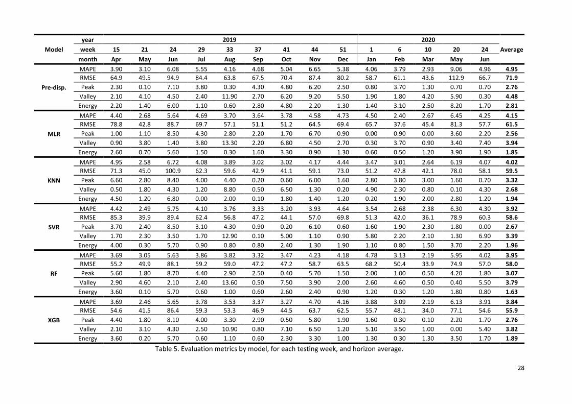
28
Model
year 2019 2020
Average week 15 21 24 29 33 37 41 44 51 1 6 10 20 24
month Apr May Jun Jul Aug Sep Oct Nov Dec Jan Feb Mar May Jun
Pre-disp.
MAPE 3.90 3.10 6.08 5.55 4.16 4.68 5.04 6.65 5.38 4.06 3.79 2.93 9.06 4.96 4.95
RMSE 64.9 49.5 94.9 84.4 63.8 67.5 70.4 87.4 80.2 58.7 61.1 43.6 112.9 66.7 71.9
Peak 2.30 0.10 7.10 3.80 0.30 4.30 4.80 6.20 2.50 0.80 3.70 1.30 0.70 0.70 2.76
Valley 2.10 4.10 4.50 2.40 11.90 2.70 6.20 9.20 5.50 1.90 1.80 4.20 5.90 0.30 4.48
Energy 2.20 1.40 6.00 1.10 0.60 2.80 4.80 2.20 1.30 1.40 3.10 2.50 8.20 1.70 2.81
MLR
MAPE 4.40 2.68 5.64 4.69 3.70 3.64 3.78 4.58 4.73 4.50 2.40 2.67 6.45 4.25 4.15
RMSE 78.8 42.8 88.7 69.7 57.1 51.1 51.2 64.5 69.4 65.7 37.6 45.4 81.3 57.7 61.5
Peak 1.00 1.10 8.50 4.30 2.80 2.20 1.70 6.70 0.90 0.00 0.90 0.00 3.60 2.20 2.56
Valley 0.90 3.80 1.40 3.80 13.30 2.20 6.80 4.50 2.70 0.30 3.70 0.90 3.40 7.40 3.94
Energy 2.60 0.70 5.60 1.50 0.30 1.60 3.30 0.90 1.30 0.60 0.50 1.20 3.90 1.90 1.85
KNN
MAPE 4.95 2.58 6.72 4.08 3.89 3.02 3.02 4.17 4.44 3.47 3.01 2.64 6.19 4.07 4.02
RMSE 71.3 45.0 100.9 62.3 59.6 42.9 41.1 59.1 73.0 51.2 47.8 42.1 78.0 58.1 59.5
Peak 6.60 2.80 8.40 4.00 4.40 0.20 0.60 6.00 1.60 2.80 3.80 3.00 1.60 0.70 3.32
Valley 0.50 1.80 4.30 1.20 8.80 0.50 6.50 1.30 0.20 4.90 2.30 0.80 0.10 4.30 2.68
Energy 4.50 1.20 6.80 0.00 2.00 0.10 1.80 1.40 1.20 0.20 1.90 2.00 2.80 1.20 1.94
SVR
MAPE 4.42 2.49 5.75 4.10 3.76 3.33 3.20 3.93 4.64 3.54 2.68 2.38 6.30 4.30 3.92
RMSE 85.3 39.9 89.4 62.4 56.8 47.2 44.1 57.0 69.8 51.3 42.0 36.1 78.9 60.3 58.6
Peak 3.70 2.40 8.50 3.10 4.30 0.90 0.20 6.10 0.60 1.60 1.90 2.30 1.80 0.00 2.67
Valley 1.70 2.30 3.50 1.70 12.90 0.10 5.00 1.10 0.90 5.80 2.20 2.10 1.30 6.90 3.39
Energy 4.00 0.30 5.70 0.90 0.80 0.80 2.40 1.30 1.90 1.10 0.80 1.50 3.70 2.20 1.96
RF
MAPE 3.69 3.05 5.63 3.86 3.82 3.32 3.47 4.23 4.18 4.78 3.13 2.19 5.95 4.02 3.95
RMSE 55.2 49.9 88.1 59.2 59.0 47.2 47.2 58.7 63.5 68.2 50.4 33.9 74.9 57.0 58.0
Peak 5.60 1.80 8.70 4.40 2.90 2.50 0.40 5.70 1.50 2.00 1.00 0.50 4.20 1.80 3.07
Valley 2.90 4.60 2.10 2.40 13.60 0.50 7.50 3.90 2.00 2.60 4.60 0.50 0.40 5.50 3.79
Energy 3.60 0.10 5.70 0.60 1.00 0.60 2.60 2.40 0.90 1.20 0.30 1.20 1.80 0.80 1.63
XGB
MAPE 3.69 2.46 5.65 3.78 3.53 3.37 3.27 4.70 4.16 3.88 3.09 2.19 6.13 3.91 3.84
RMSE 54.6 41.5 86.4 59.3 53.3 46.9 44.5 63.7 62.5 55.7 48.1 34.0 77.1 54.6 55.9
Peak 4.40 1.80 8.10 4.00 3.30 2.90 0.50 5.80 1.90 1.60 0.30 0.10 2.20 1.70 2.76
Valley 2.10 3.10 4.30 2.50 10.90 0.80 7.10 6.50 1.20 5.10 3.50 1.00 0.00 5.40 3.82
Energy 3.60 0.20 5.70 0.60 1.10 0.60 2.30 3.30 1.00 1.30 0.30 1.30 3.50 1.70 1.89
Table 5. Evaluation metrics by model, for each testing week, and horizon average.

29
The weekly evaluation demonstrates that XGB improved MAPE and RMSE for all the testing weeks.
XGB was also accurate in predicting the peak load, valley load, and weekly energy. MLR is the simplest,
but it also showed the smallest peak deviation overall, followed by SVR. KNN did not expose this issue,
but it predicted unusual hourly load profiles on holidays. It also tends to forecast lower demands. For
instance, it was the best model to predict load valleys, followed by SVR, but the worst to predict load
peaks. RF showed a good performance for peaks and valleys and had the smallest energy deviation
along all testing weeks, followed by XGB. The RF forecast’s negative side was the irregular spikes that
do not follow the typical hourly profile. In general, all algorithms were benefited by hybridization by
improving holidays’ forecast. Mostly MLR, since it solely, could not predict lower demands for holidays.
Since XGB demonstrated the best performance, providing an average MAPE of 3.84% and an RMSE of
55.9 MWh, only hourly results from this model are plotted along with the pre-dispatch forecast, and
the real load, illustrated in Figure 5. These testing weeks include holidays, regular days, and periods
with quarantine restrictions due to the COVID-19 pandemic. Figure 6 shows another testing week, with
all the candidates’ ML models forecast.
(a)
(b)
(c)
Figure 5. Pre-dispatch and XGB forecast comparison with the real load. (a) Week 51, 2019 (21st to 27th, Dec 2019); (b) Week 10, 2020 (7th to 13th, Mar 2019); (c) Week 24, 2020 (13th to 19th, Jun 2020)
800
1000
1200
1400
1600
1800
1 7 13 19 25 31 37 43 49 55 61 67 73 79 85 91 97 103 109 115 121 127 133 139 145 151 157 163
Sat Sun Mon Tue Wed Thu Fri
Load
(M
Wh
)
Pre-Dispatch Real Load
800
1000
1200
1400
1600
1800
1 7 13 19 25 31 37 43 49 55 61 67 73 79 85 91 97 103 109 115 121 127 133 139 145 151 157 163
Sat Sun Mon Tue Wed Thu Fri
Load
(M
Wh
)
Pre-Dispatch Real Load
800
1000
1200
1400
1600
1800
1 7 13 19 25 31 37 43 49 55 61 67 73 79 85 91 97 103 109 115 121 127 133 139 145 151 157 163
Sat Sun Mon Tue Wed Thu Fri
Load
(M
Wh
)
Pre-Dispatch Real Load

30
Overall, all models distinguished between weekends and weekdays load. Since weekends had a lower
demand with low variance, all models showed a decent performance for these periods. For periods
with similar characteristics, like the early morning, most of the forecasts were reasonably good. The
most difficult hours to forecast were daytime periods during working days due to their high variance.
The most challenging was holidays due to fewer records, different contexts, and the natural
randomness of consumers’ demand. Examples of holiday forecasting are shown in Figure 5a, on
Tuesday 24 and Wednesday 25 December 2019, and another holiday example is illustrated in Figure
6a for Thursday 18 and Friday 19 April 2019. The quarantine period brings another challenge for STLF
task since the load profiles changed abruptly for this period, and fewer records are available for
training. Besides, the load profiles do not follow a steady pattern. Differences between the quarantine
period and no quarantine are shown in Figure 5b, c, respectively.
(a)
(b)
Figure 6. Weekly pre-dispatch vs. ML candidates’ models. (a) Hourly forecast for Week 15, 2019 (13th to 19th, Apr 2019); (b) Frequency distribution of error by forecast, for Week 15, Apr 2019.
4.2. FEATURE IMPORTANCE RESULTS
Beyond having an accurate forecast, it is relevant to know the factors contributing to a specific STLF
task. Some of the ML candidates’ models proposed in this project provide a straightforward way to
check the feature importance, except for KNN and SVR, which only provide coefficients for the linear
kernel. Still, feature permutation importance (Raschka, 2021) is applied to those two models with ten
permutation rounds to estimate their feature importance. For MLR, feature importance is obtained
through the coefficient property by multiplying each coefficient by the feature standard deviation to
reduce all coefficients to the same measurement unit. Each feature’s absolute value is then scaled to
get the contribution percentage. For RF and XGB, the feature importance property directly returns
contribution percentage by feature. Table 6 shows the feature importance by ML model, where each
value is the average from evaluating each model on the 14 testing weeks.
800
1000
1200
1400
1600
1800
1 7 13 19 25 31 37 43 49 55 61 67 73 79 85 91 97 103 109 115 121 127 133 139 145 151 157 163
Sat Sun Mon Tue Wed Thu Fri
Load
(M
Wh
)
Real Load Pre-Dispatch MLR KNN SVR RF XGB
0
5
10
15
20
25
30
−354−322−290−258−226−194−162−130 −98 −66 −34 −2 30 62 94 126 158 190
Freq
uen
cy
Error (MWh)
MLR
KNN
SVR
RF
XGB
Pre-Dispatch

31
Feature Regular days' model Holidays' model
MLR KNN SVR RF XGB MLR KNN SVR RF XGB
𝐿𝒉−𝟑𝟑𝟔 6.91 3.04 1.84 0.83 16.14 11.28 12.17 5.50 4.91 11.22
𝐿𝒉−𝟓𝟎𝟒 7.19 2.73 2.10 0.81 11.83 12.49 7.08 7.77 3.52 5.70
𝐿𝒉−𝟔𝟕𝟐 6.70 3.99 2.58 0.68 14.29 10.81 3.01 3.38 2.72 9.81
𝐿𝑀𝐴𝒉(1,4) 57.43 10.52 70.55 89.51 25.56 53.21 22.45 50.57 54.15 20.47
𝑑𝑎𝑦_𝑜𝑓_𝑡ℎ𝑒_𝑤𝑒𝑒𝑘𝒉 0.56 4.43 1.74 0.41 1.66 0.36 21.27 12.43 7.19 8.97
𝑤𝑒𝑒𝑘𝑒𝑛𝑑_𝑖𝑛𝑑𝑖𝑐𝑎𝑡𝑜𝑟𝒉 2.43 18.31 5.47 0.10 4.76 3.54 8.72 8.84 0.30 5.72
ℎ𝑜𝑙𝑖𝑑𝑎𝑦_𝑖𝑛𝑑𝑖𝑐𝑎𝑡𝑜𝑟𝒉 9.13 18.53 7.00 2.15 7.85 - - - - -
ℎ𝑜𝑙𝑖𝑑𝑎𝑦_𝐼𝐷𝒉 1.65 1.40 0.46 2.63 2.41 1.77 1.04 1.49 14.83 12.64
ℎ𝑜𝑢𝑟_𝑜𝑓_𝑡ℎ𝑒_𝑑𝑎𝑦𝒉 1.69 17.59 2.50 0.70 10.56 6.06 19.87 5.11 7.46 21.72
𝑡𝑒𝑚𝑝_𝑃𝑎𝑛𝑎𝑚𝑎_𝑐𝑖𝑡𝑦𝒉 6.31 19.44 5.76 2.17 4.94 0.48 4.38 4.92 4.90 3.75
Table 6. Average feature importance by ML model expressed in percentage (%).
The feature importance results show that the load’s lags, and consequently, the moving average, have
a strong influence on the forecasting. Feature importance differs by model, showing that XGB has the
most balanced features’ contribution. A significant difference between regular and holidays’ model is
that the holidays’ model has a more considerable contribution from holiday_ID and hour of the day,
making this model specialized on holidays. The hour of the day is also a crucial feature for regular days’
model, especially for KNN; also, temperature resulted in an essential feature for KNN, but as a
secondary feature for the rest of the models. Lastly, the binary indicators for holidays and weekends
show minor importance but still relevant, mainly to mark the difference between a higher load peak
for working days and a lower peak for non-working days.
4.3. HYPERPARAMETER SEARCH RESULTS
The hyperparameter search results for regular days’ models and holidays’ models are shown in Table
7 and Table 8, respectively, except for MLR, which does not possess a hyperparameter space to
enhance the predictions. As exposed, XGB demonstrated the best performance; for this reason, only a
description of these parameters will be addressed. For the ‘eval_metric’ parameter, ‘rmse’ was the
most suitable option to penalize large errors. The default ‘gbtree’ booster was kept to take advantage
of the generalization ability of the ensemble of trees instead of the weighted sum of linear functions
provided by ‘gblinear’. The ‘n_estimators’ is the number of iterations the model will perform, in which
a new tree is created per iteration. For this reason, values above hundreds of trees are considered to
make a sizeable iterative process that can adapt to the problem. The ‘max_depth’ parameter was kept
with low values to avoid overfitting by training weak tree learners. The ‘learning_rate’ had the most
extensive search to adapt the hyperparameter search during each boosting step, preventing
overfitting. The parameters ‘subsample’, ‘colsample_bytree’, ‘colsample_bynode’, and
‘col_sample_bylevel’ were reduced to provide generalization ability to the model, restricting the
training process with sub-samples of the data. A range of larger values and the default zero were
explored for ’gamma’, to control partitions on the leaves’ nodes, making the algorithm more
conservative. Similarly, because ‘min_child_weight’ controls the number of instances needed to be in
each node, for this reason, values above the zero-default setting were explored. A log-uniform
distribution with values lower than five was considered for ‘alpha’ and ‘lambda’, aiming to add a small
bias to make the model conservative and avoid overfitting.

32
Model
year 2019 2020
week no. 15 21 24 29 33 37 41 44 51 1 6 10 20 24
month Apr May Jun Jul Aug Sep Oct Nov Dec Jan Feb Mar May Jun
KNN
n_neighbors 41 31 31 31 41 31 31 37 31 37 37 31 29 35
weights dist. dist dist dist dist dist dist dist dist dist dist dist dist dist
metric manht. manht. manht. manht. manht. manht. manht. manht. manht. manht. manht. manht. manht. manht.
leaf_size 11 1 1 1 16 16 1 46 46 1 16 16 21 46
SVR
kernel rbf rbf rbf rbf rbf rbf rbf rbf rbf rbf rbf rbf rbf rbf
epsilon 2.48927 8.25782 0.00082 0.01421 0.00033 0.00092 0.02024 0.86639 0.00013 6.93334 0.00014 0.02678 7.16092 0.02286
C 415.13 409.21 299.93 304.05 318.07 332.74 331.23 367.35 315.65 2938.91 296.54 307.96 243.53 308.42
tol 0.00694 0.00350 0.00868 0.00780 0.00853 0.00811 0.00012 0.00876 0.00024 0.00931 0.00293 0.00772 0.00072 0.00882
RF
n_estimators 140 140 100 80 120 200 180 180 200 180 200 200 200 180
max_samples 0.60 0.65 0.70 0.70 0.60 0.65 0.70 0.70 0.65 0.65 0.60 0.60 0.60 0.60
max_depth 10 10 10 13 13 13 10 13 13 10 13 13 10 10
ccp_alpha 1.59×10⁻⁴ 2.33×10⁻⁶ 2.86×10⁻⁵ 1.50×10⁻⁵ 9.16×10⁻⁵ 9.83×10⁻⁴ 3.87×10⁻⁶ 1.68×10⁻⁴ 1.19×10⁻⁶ 8.10×10⁻⁵ 1.73×10⁻⁵ 3.65×10⁻⁶ 3.54×10⁻⁴ 9.72×10⁻⁴
XGB
n_estimators 350 400 350 400 500 400 600 550 350 600 500 600 600 550
max_depth 5 4 4 5 4 5 4 5 5 5 5 5 4 4
subsample 0.75 0.75 0.70 0.65 0.65 0.75 0.65 0.65 0.60 0.75 0.75 0.65 0.70 0.75
colsample_bytree 0.75 0.70 0.65 0.80 0.70 0.60 0.75 0.80 0.60 0.60 0.70 0.70 0.75 0.65
colsample_bylevel 0.70 0.90 0.80 0.65 0.70 0.85 0.80 0.60 0.75 0.60 0.90 0.65 0.85 0.85
colsample_bynode 0.70 0.75 0.80 0.60 0.65 0.70 0.90 0.60 0.90 0.70 0.85 0.85 0.75 0.75
learning_rate 0.050016 0.066828 0.057397 0.030956 0.051173 0.039766 0.036783 0.022305 0.052250 0.041089 0.042121 0.027303 0.027487 0.021568
min_child_weight 7 3 3 7 7 1 7 3 5 3 1 7 7 3
gamma 1.7696 0.9889 0.0440 0.1366 0.0039 5.81×10⁻⁵ 1.65×10⁻³ 1.71×10⁻⁴ 0.9251 7.12×10⁻⁴ 0.0220 1.34×10⁻³ 1.35×10⁻⁵ 0.8903
lambda 1.1940 1.4665 3.1788 1.1477 3.6228 3.6026 2.5763 1.6005 3.2689 3.7203 2.6808 1.7332 1.0280 3.6871
alpha 1.0194 0.1336 0.0457 0.0209 2.94×10⁻³ 0.0183 3.00×10⁻³ 4.55×10⁻⁴ 0.0338 7.46×10⁻⁵ 7.47×10⁻⁴ 9.20×10⁻⁵ 0.0738 0.2525
Table 7. Hyperparameter optimization results for regular days’ models, by testing week.

33
Model
year 2019 2020
week no. 15 21 24 29 33 37 41 44 51 1 6 10 20 24
month Apr May Jun Jul Aug Sep Oct Nov Dec Jan Feb Mar May Jun
KNN
n_neighbors 25 25 33 21 15 27 21 15 39 39 21 29 21 29
weights dist. dist dist dist dist dist dist dist dist dist dist dist dist dist
metric manht. manht. manht. manht. manht. manht. manht. manht. manht. manht. manht. manht. manht. manht.
leaf_size 1 11 1 26 46 26 21 1 26 6 46 16 11 26
SVR
kernel rbf rbf rbf rbf rbf rbf rbf rbf rbf rbf rbf rbf rbf rbf
epsilon 0.00264 0.00045 0.00017 9.45318 6.31538 1.09855 5.73192 0.00023 0.20928 0.90036 2.22753 8.30718 0.00029 0.62205
C 2802.99 626.41 460.37 807.35 303.19 257.51 609.51 248.33 149.49 151.74 142.09 111.01 2774.43 234.76
tol 0.00794 0.00852 0.00967 0.00998 0.00185 0.00361 0.00556 0.00671 0.00540 0.00417 0.00991 0.00606 0.00321 0.00592
RF
n_estimators 100 100 140 200 100 200 100 200 80 100 140 140 100 100
max_samples 0.80 0.80 0.80 0.60 0.80 0.80 0.80 0.80 0.60 0.80 0.80 0.80 0.80 0.80
max_depth 19 13 19 16 16 16 16 19 19 13 19 19 16 19
ccp_alpha 2.24×10⁻⁵ 5.31×10⁻⁵ 1.51×10⁻⁶ 4.70×10⁻⁵ 6.03×10⁻⁵ 8.83×10⁻⁴ 2.24×10⁻⁵ 4.45×10⁻⁵ 2.09×10⁻⁵ 2.84×10⁻⁴ 7.46×10⁻⁶ 4.46×10⁻⁵ 8.40×10⁻⁶ 1.06×10⁻⁴
XGB
n_estimators 300 500 500 300 500 300 500 500 300 450 350 450 500 300
max_depth 4 6 4 5 7 4 7 4 6 7 4 6 4 7
subsample 0.80 0.90 0.60 0.80 0.75 0.80 0.70 0.75 0.90 0.70 0.80 0.70 0.60 0.85
colsample_bytree 0.70 0.90 0.90 0.65 0.75 0.60 0.60 0.80 0.90 0.65 0.80 0.65 0.70 0.90
colsample_bylevel 0.80 0.90 0.90 0.80 0.90 0.80 0.90 0.90 0.70 0.90 0.80 0.90 0.80 0.80
colsample_bynode 0.90 0.80 0.90 0.90 0.90 0.90 0.80 0.70 0.90 0.80 0.80 0.90 0.90 0.60
learning_rate 0.059702 0.022990 0.099259 0.096232 0.058822 0.046665 0.026215 0.046144 0.096558 0.031292 0.072094 0.090842 0.065184 0.090743
min_child_weight 5 3 7 3 3 5 5 5 7 7 7 3 3 3
gamma 2.86×10⁻³ 1.47×10⁻³ 0.0464 6.64×10⁻⁴ 2.29×10⁻³ 0.5343 3.46×10⁻⁵ 2.52×10⁻³ 1.20×10⁻⁵ 3.40×10⁻⁵ 1.8331 0.4352 1.93×10⁻⁵ 0.0833
lambda 3.6348 1.2237 1.1215 1.0615 1.6029 1.4756 3.2333 4.3853 1.6743 1.0481 1.2192 2.0430 1.6593 1.7202
alpha 4.44×10⁻⁵ 2.85×10⁻³ 1.11×10⁻³ 3.07×10⁻⁴ 6.56×10⁻⁴ 1.99×10⁻⁵ 8.60×10⁻⁵ 1.61×10⁻³ 9.33×10⁻⁵ 1.06×10⁻⁴ 1.62×10⁻⁴ 4.51×10⁻³ 9.24×10⁻⁴ 6.46×10⁻⁴
Table 8. Hyperparameter optimization results for holidays’ models, by testing week.

34
4.4. BENCHMARKING
The results obtained in this project can be interpreted from the perspective of any time-series
forecasting research using ML techniques since the standard ML methodologies for STLF were applied
to train and evaluate results, as exposed in the literature review. For example, the selected features
across the STLF field of study match this project’s best features: the load’s lags, the hour of the day,
and temperature. Holidays and weekends’ binary indicators also contribute since they help determine
a high or low load range.
In contrast with most of the studies where researchers forecast 24 or 48 hours, this project addressed
a 168-hour horizon, considering a 72-hour gap before the first forecasting period. A second
differentiation is the implementation of a hybrid model to enhance the holidays’ forecast; within the
weekly forecasting horizon. Besides the typical MAPE and RMSE evaluation metrics, this project
proposed load peak, load valley, and energy evaluation as secondary, practical metrics that analysts
can easily monitor. Another distinction of this project is the diversity for testing periods, presenting
STLF for regular working days, holidays, and irregular periods during the 2020 quarantine. This project’s
most important distinction is comparing the official weekly pre-dispatch forecast as a baseline and
validating the results.
As exposed in the introduction section, this project’s direct implication is forecasting Panama’s
national load. However, these models can be trained and applied to countries or regions with similar
conditions.

35
5. CONCLUSIONS
This project’s main objectives were to evaluate current Panama’s official load forecast and develop a
set of Machine Learning models to improve this official load forecast. For instance, the models were
developed and benchmarked with data and previous forecasts from Panama’s power system. This
project presented a novel hybrid methodology to improve the weekly STLF forecast for the Panama
case study to address the forecasting task, keeping a 72-hour gap. A set of five proven algorithms
across the research field were chosen to develop the hybrid models and subsequently compare their
results against the official forecasting tool records on diverse testing weeks. Results along 14 testing
weeks confirmed the suitability of the XGB algorithm for the hybrid methodology. First, for time
efficiency on training and predicting; second, for flexibility due to the parameter space; and third, for
the ease of providing certain interpretability through its feature importance property.
For the above-exposed reasons, this project makes several significant contributions to the field of
study. First, it shows that models built with XGB have superior performance to models built with other
algorithms. Second, it confirms that temperature plays an important role in STLF. Third, it
demonstrates the excellent performance of ML models by forecasting for a longer horizon than typical
research; and even with a three-day gap of data before the forecast. Lastly, this project identifies public
data that other researchers can use to improve a framed forecasting task. Details about this project
dataset repository are available in Appendix 1.
This project also has several practical implications. The first and main implication is to replace the
current forecasting tool for the Panama case study, thus allowing Panama to reduce costs and improve
STLF performance. Second, this model could be trained and applied in other countries or regions with
similar conditions. Furthermore, the positive impacts of providing a more accurate STLF will reduce
the planning uncertainty added by the intermittent renewable production and subsequently be closer
to the optimal hydro-thermal costs scheduled in the weekly unit commitment. This third practical
implication leads to a fourth: for the specific case of the Panama energy spot market, because it is a
marginalist market, accurate STLF can also reduce the hourly energy price uncertainty in the wholesale
electricity market.

36
6. LIMITATIONS AND RECOMMENDATIONS FOR FUTURE WORKS
Future work within this specific research can include more historical load records to train models in
particular situations, like holidays. Another approach to enhance forecasts is to classify load profiles
using clustering techniques prior training (Zheng et al., 2017), and use stacking techniques to enhance
the forecast accuracy, even though it increases the training and predicting time (Massaoudi et al.,
2021).
In the particular case study of Panama’s national load, there are special consumers named auto-
generators: the Panama Canal and Minera Panama (CND, 2021a). These consumers have a significant
load, but as their agent’s name suggests, they supply their own demand with their own power plants
most of the time, except for scheduled maintenance periods on their power plants or unforeseen
unavailability on their power plants (CND, 2021d). Those agents will consume energy from the national
power system during those events, causing an extra increase in the national load. If this additional load
can be scheduled, it is better to track the electricity load by consumer and forecast only the residential,
commercial, and industrial load, then add auto-generators if needed. This load segregation avoids
distortions on the load forecast, as stated in auto-generators methodology (CND, 2021b). In this
context, another research avenue to develop STLF by consumers emerges, but it requires data with
this segregation.
Since DL models are out of this project scope, and DL models require more records than ML models,
unidirectional and bidirectional LSTM were not compared in the research. However, future studies
should evaluate these algorithms’ performance that have proven good for STLF (Atef & Eltawil, 2020).
Similarly, non-iterative ANN-based algorithms can be explored due to their good performance and low
training time, like (Vitynskyi et al., 2018) compared with a set of ML models.
Although there are currently several weather forecasts available with hourly granularity (Visual
Crossing, 2021), because the temperature is crucial for STLF, it is advisable to count with an accurate
temperature forecast to feed this STLF model. Hence, a temperature forecast model can complement
this project.
It is advised to do a weekly load patterns revision since consumption patterns can change in the future.
An example of abrupt changes on the hourly load profile was exposed in this project during the 2020
quarantine period. However, other trending consumption patterns (Andersen et al., 2019), like
recharging more electric vehicles and having more solar production behind-the-meter, will produce
residential and commercial hourly consumption changes. This revision implies that forecasting models
should be updated more often, and even that they need to be more robust.
A possible solution to overcome these issues is to automatically enable the models to learn with new
data every week by deploying the “Champion-Challenger” approach (Abbott, 2014). A weekly
hyperparameter tuning is executed to update the models and make them compete to ensure the best
performance along time.
The final goal of STLF is to reduce the uncertainty on real-time dispatch of hydro-thermal power plants
because the wind and solar farms are non-dispatchable power plants. Consequently, another way to
reduce the planning uncertainty and complement the STLF is by providing an accurate forecast for
wind and solar production and other non-dispatchable power plants, if any.

37
7. BIBLIOGRAPHY
Abbasimehr, H., Shabani, M., & Yousefi, M. (2020). An optimized model using LSTM network for
demand forecasting. Computers and Industrial Engineering, 143(July 2019), 106435.
https://doi.org/10.1016/j.cie.2020.106435
Abbott, D. (2014). Applied Predictive Analytics. Principles and techniques for the professional data
analyst. (p. 372). Indianapolis, IN, USA: John Wiley & Sons, Inc.
Adeoye, O., & Spataru, C. (2019). Modelling and forecasting hourly electricity demand in West
African countries. Applied Energy, 242(March), 311–333.
https://doi.org/10.1016/j.apenergy.2019.03.057
Aguilar Madrid, E., & Valdés Bosquez, L. (2017). Impact of wind and photovoltaic generation input in
Panama ; Impacto de la entrada de la generación eólica y fotovoltaica en Panamá. I+D
Tecnológico, 13(1), 71-82. Retrieved from https://revistas.utp.ac.pa/index.php/id-
tecnologico/article/view/1440
Akiba, T., Sano, S., Yanase, T., Ohta, T., & Koyama, M. (2019). Optuna: A next-generation
hyperparameter optimization framework. ArXiv, 2623–2631.
https://doi.org/10.1145/3292500.3330701
Al-Musaylh, M. S., Deo, R. C., Adamowski, J. F., & Li, Y. (2018). Short-term electricity demand
forecasting with MARS, SVR and ARIMA models using aggregated demand data in Queensland,
Australia. Advanced Engineering Informatics, 35(November 2017), 1–16.
https://doi.org/10.1016/j.aei.2017.11.002
Alex J., S., & Schölkopf, B. (2004). A tutorial on support vector regression. Statistics and Computing,
14, 199–222. http://dx.doi.org/10.1088/1751-8113/44/8/085201
Amin, M. A. Al, & Hoque, M. A. (2019). Comparison of ARIMA and SVM for short-term load
forecasting. IEMECON 2019 - 9th Annual Information Technology, Electromechanical
Engineering and Microelectronics Conference, 205–210.
https://doi.org/10.1109/IEMECONX.2019.8877077
Amjady, N. (2001). Short-term hourly load forecasting using time-series modeling with peak load
estimation capability. IEEE Transactions on Power Systems, 16(4), 798–805.
https://doi.org/10.1109/59.962429
Andersen, F. M., Henningsen, G., Møller, N. F., & Larsen, H. V. (2019). Long-term projections of the
hourly electricity consumption in Danish municipalities. Energy, 186, 115890.
https://doi.org/10.1016/j.energy.2019.115890
Atef, S., & Eltawil, A. B. (2020). Assessment of stacked unidirectional and bidirectional long short-
term memory networks for electricity load forecasting. Electric Power Systems Research,
187(April), 106489. https://doi.org/10.1016/j.epsr.2020.106489
Barakat, E. H., & Al-Qasem, J. M. (1998). Methodology for weekly load forecasting. IEEE Transactions
on Power Systems, 13(4), 1548–1555. https://doi.org/10.1109/59.736304

38
Becirovic, E., & Cosovic, M. (2016). Machine learning techniques for short-Term load forecasting. 4th
International Symposium on Environment Friendly Energies and Applications, EFEA 2016.
https://doi.org/10.1109/EFEA.2016.7748789
Bergstra, J., Bardenet, R., Bengio, Y., & Kégl, B. (2011). Algorithms for hyper-parameter optimization.
Advances in Neural Information Processing Systems 24: 25th Annual Conference on Neural
Information Processing Systems 2011, NIPS 2011, 1–9. Retrieved from
https://papers.nips.cc/paper/2011/file/86e8f7ab32cfd12577bc2619bc635690-Paper.pdf
Bertsimas, D., Delarue, A., Jaillet, P., & Martin, S. (2019). The Price of Interpretability.
https://arxiv.org/abs/1907.03419
Boya, C. (2019). Analyzing the relationship between temperature and load demand in the regions
with the highest electricity consumption in the republic of Panama. Proceedings - 2019 7th
International Engineering, Sciences and Technology Conference, IESTEC 2019, 132–137.
https://doi.org/10.1109/IESTEC46403.2019.00-88
Cai, J., Cai, H., Cai, Y., Wu, L., & Shen, Y. (2020). Short-term Forecasting of User Power Load in China
Based on XGBoost. 3, 1–5. https://doi.org/10.1109/appeec48164.2020.9220335
Cai, Y., Xie, Q., Wang, C., & Lu, F. (2011). Short-term load forecasting for city holidays based on
genetic support vector machines. 2011 International Conference on Electrical and Control
Engineering, ICECE 2011 - Proceedings, 1, 3144–3147.
https://doi.org/10.1109/ICECENG.2011.6057627
Cao, L., Li, Y., Zhang, J., Jiang, Y., Han, Y., & Wei, J. (2020). Electrical load prediction of healthcare
buildings through single and ensemble learning. Energy Reports, 6, 2751–2767.
https://doi.org/10.1016/j.egyr.2020.10.005
Chapagain, K., & Kittipiyakul, S. (2018). Short-Term Electricity Demand Forecasting with Seasonal and
Interactions of Variables for Thailand. IEECON 2018 - 6th International Electrical Engineering
Congress, March 2009, 2018–2021. https://doi.org/10.1109/IEECON.2018.8712189
CND-sitr. (2021, March 2). Sistema de Información en Tiempo Real. Retreived from
http://sitr.cnd.com.pa/m/pub/sin.html
CND. (2021a, March 2). Informe de Planeamiento Operativo - Semestre I 2020. Retreived from
https://sitioprivado.cnd.com.pa/Informe/Download/36121?key=VXd9e23Z9JRA5aIUR21R-
P8gocoGOMqdvSo79FduN
CND. (2021b, March 2). Metodologías de Detallle (enero 2021). Metodologías de Detalle. Retreived
from https://www.cnd.com.pa/index.php/acerca/documentos/normas
CND. (2021c, March 2). Post-dispatch – Operations Reports. Retrieved from
https://www.cnd.com.pa/index.php/informes/categoria/informes-de-operaciones?tipo=60
CND. (2021d, March 2). Reglas Comerciales. Reglas Comerciales Para El Mercado Mayorista de
Electricidad. Retreived from https://www.cnd.com.pa/index.php/acerca/documentos/normas

39
CND. (2021e, March 2). Weekly pre-dispatch – Operations Reports. Retreived from
https://www.cnd.com.pa/index.php/informes/categoria/informes-de-
operaciones?tipo=68&anio=2019&semana=0
Dietrich, B., Walther, J., Weigold, M., & Abele, E. (2020). Machine learning based very short term
load forecasting of machine tools. Applied Energy, 276(February), 115440.
https://doi.org/10.1016/j.apenergy.2020.115440
Dietvorst, B. J., Simmons, J. P., & Massey, C. (2015). Algorithm aversion: People erroneously avoid
algorithms after seeing them err. Journal of Experimental Psychology: General, 144(1), 114–126.
https://doi.org/10.1037/xge0000033
Do, L. P. C., Lin, K. H., & Molnár, P. (2016). Electricity consumption modelling: A case of Germany.
Economic Modelling, 55, 92–101. https://doi.org/10.1016/j.econmod.2016.02.010
Dutta, S., Li, Y., Venkataraman, A., Costa, L. M., Jiang, T., Plana, R., Tordjman, P., Choo, F. H., Foo, C.
F., & Puttgen, H. B. (2017). Load and Renewable Energy Forecasting for a Microgrid using
Persistence Technique. Energy Procedia, 143, 617–622.
https://doi.org/10.1016/j.egypro.2017.12.736
Eseye, A. T., Lehtonen, M., Tukia, T., Uimonen, S., & Millar, R. J. (2019). Machine Learning Based
Integrated Feature Selection Approach for Improved Electricity Demand Forecasting in
Decentralized Energy Systems. IEEE Access, 7, 91463–91475.
https://doi.org/10.1109/ACCESS.2019.2924685
Fernandes, R. S. S., Bichpuriya, Y. K., Rao, M. S. S., & Soman, S. A. (2011). Day ahead load forecasting
models for holidays in Indian context. 2011 International Conference on Power and Energy
Systems, ICPS 2011, 1–5. https://doi.org/10.1109/ICPES.2011.6156652
Ferreira, P. M., Cuambe, I. D., Ruano, A. E., & Pestana, R. (2013). Forecasting the Portuguese
electricity consumption using least-squares support vector machines. IFAC Proceedings Volumes
(IFAC-PapersOnline), 3(PART 1), 411–416. https://doi.org/10.3182/20130902-3-CN-3020.00138
Ferreira, P. M., Ruano, A. E., & Pestana, R. (2010). Improving the identification of RBF predictive
models to forecast the Portuguese electricity consumption ? IFAC Proceedings Volumes (IFAC-
PapersOnline), 1(PART 1), 208–213. https://doi.org/10.3182/20100329-3-pt-3006.00039
Gaceta. (2020). Busqueda Avanzada Gaceta. Gaceta Oficial. Retreived from
https://www.gacetaoficial.gob.pa/Busqueda-Avanzada
GCP. (2021). AI Platform Notebooks | Google Cloud Platform. Retrieved from
https://cloud.google.com/ai-platform-notebooks
GES DISC. (2015). Global Modeling and Assimilation Office (GMAO) (2015), MERRA-2
tavg1_2d_slv_Nx: 2d,1-Hourly,Time-Averaged,Single-Level,Assimilation,Single-Level Diagnostics
V5.12.4, Greenbelt, MD, USA. Changes; Global Modeling and Assimilation Office (GMAO).
https://doi.org/10.5067/VJAFPLI1CSIV

40
Google. (2020). Colaboratory – Google. Colaboratory Frequently Asked Questions. Retrieved from
https://research.google.com/colaboratory/faq.html
Hadri, S., Naitmalek, Y., Najib, M., Bakhouya, M., Fakhri, Y., & Elaroussi, M. (2019). A comparative
study of predictive approaches for load forecasting in smart buildings. Procedia Computer
Science, 160, 173–180. https://doi.org/10.1016/j.procs.2019.09.458
Han, J., Kamber, M., & Pei, J. (2011). Data Mining. Concepts and Techniques, 3rd Edition, pp. 99-110
(The Morgan Kaufmann Series in Data Management Systems).
Herman-Saffar, O. (2021, March 2). Time Based Cross Validation. Time Based Cross Validation.
Retrieved from https://towardsdatascience.com/time-based-cross-validation-d259b13d42b8
HITACHI-ABB. (2021, March 2). Nostradamus. Short-term renewable, demand and price forecasting.
Retrieved from https://www.hitachiabb-powergrids.com/cn/en/offering/product-and-
system/energy-portfolio-management/trading-and-risk-management/nostradamus
Hossein, S., & Mohammad, S. S. (2011). Electric Power System Planning. (p. 10). Berlin, Heidelberg,
Germany: Springer.
Hoyer, S., & Hamman, J. J. (2017). xarray: N-D labeled Arrays and Datasets in Python. Journal of Open
Research Software, 5. https://doi.org/10.5334/jors.148
Johannesen, N. J., Kolhe, M., & Goodwin, M. (2019). Relative evaluation of regression tools for urban
area electrical energy demand forecasting. Journal of Cleaner Production, 218, 555–564.
https://doi.org/10.1016/j.jclepro.2019.01.108
Khwaja, A. S., Anpalagan, A., Naeem, M., & Venkatesh, B. (2020). Joint bagged-boosted artificial
neural networks: Using ensemble machine learning to improve short-term electricity load
forecasting. Electric Power Systems Research, 179(June 2019), 106080.
https://doi.org/10.1016/j.epsr.2019.106080
La Estrella de Panamá. (2021, March 2). Cuarentena en Panamá. Calles Desiertas En El Primer Día de
Cuarentena Total En Panamá Por COVID-19. Retreived from
https://www.laestrella.com.pa/nacional/200325/calles-desiertas-primer-dia-cuarentena-total-
panama-covid-19
Lebotsa, M. E., Sigauke, C., Bere, A., Fildes, R., & Boylan, J. E. (2018). Short term electricity demand
forecasting using partially linear additive quantile regression with an application to the unit
commitment problem. Applied Energy, 222(December 2017), 104–118.
https://doi.org/10.1016/j.apenergy.2018.03.155
Li, C. (2020). Designing a short-term load forecasting model in the urban smart grid system. Applied
Energy, 266(January), 114850. https://doi.org/10.1016/j.apenergy.2020.114850
Liao, X., Cao, N., Li, M., & Kang, X. (2019). Research on Short-Term Load Forecasting Using XGBoost
Based on Similar Days. Proceedings - 2019 International Conference on Intelligent
Transportation, Big Data and Smart City, ICITBS 2019, 675–678.
https://doi.org/10.1109/ICITBS.2019.00167

41
Liu, F., Findlay, R. D., & Song, Q. (2006). A neural network based short term electric load forecasting
in Ontario Canada. CIMCA 2006: International Conference on Computational Intelligence for
Modelling, Control and Automation, Jointly with IAWTIC 2006: International Conference on
Intelligent Agents Web Technologies ..., 0–6. https://doi.org/10.1109/CIMCA.2006.17
Liu, X., Zhang, Z., & Song, Z. (2020). A comparative study of the data-driven day-ahead hourly
provincial load forecasting methods: From classical data mining to deep learning. Renewable
and Sustainable Energy Reviews, 119(November 2019), 109632.
https://doi.org/10.1016/j.rser.2019.109632
Liu, Y., Luo, H., Zhao, B., Zhao, X., & Han, Z. (2019). Short-Term Power Load Forecasting Based on
Clustering and XGBoost Method. Proceedings of the IEEE International Conference on Software
Engineering and Service Sciences, ICSESS, 2018-Novem, 536–539.
https://doi.org/10.1109/ICSESS.2018.8663907
Massaoudi, M., Refaat, S. S., Chihi, I., Trabelsi, M., Oueslati, F. S., & Abu-Rub, H. (2021). A novel
stacked generalization ensemble-based hybrid LGBM-XGB-MLP model for Short-Term Load
Forecasting. Energy, 214, 118874. https://doi.org/10.1016/j.energy.2020.118874
McKinney, W., & Team, P. D. (2020). pandas: powerful Python data analysis toolkit Release 1.1.4.
https://doi.org/10.5281/zenodo.3509134
Morales-España, G., Latorre, J. M., & Ramos, A. (2013). Tight and compact MILP formulation of start-
up and shut-down ramping in unit commitment. IEEE Transactions on Power Systems, 28(2),
1288–1296. https://doi.org/10.1109/TPWRS.2012.2222938
Nadh, K. (2021, March 2). netCDF4 API documentation. NetCDF4 API Documentation. Retrieved from
https://unidata.github.io/netcdf4-python/
Omidi, A., Barakati, S. M., & Tavakoli, S. (2015). Application of nusupport vector regression in short-
term load forecasting. 20th Electrical Power Distribution Conference, EPDC 2015, April, 32–36.
https://doi.org/10.1109/EPDC.2015.7330469
Optuna. (2021a, March 2). TPE Sampler — Optuna 2.5.0 documentation. Retreived from
https://optuna.readthedocs.io/en/stable/reference/generated/optuna.samplers.TPESampler.ht
ml
Optuna. (2021b, March 2). Trial — Optuna 2.5.0 documentation. Retreived from
https://optuna.readthedocs.io/en/stable/reference/generated/optuna.trial.Trial.html
Paterakis, N. G., Mocanu, E., Gibescu, M., Stappers, B., & Van Alst, W. (2017). Deep learning versus
traditional machine learning methods for aggregated energy demand prediction. 2017 IEEE PES
Innovative Smart Grid Technologies Conference Europe, ISGT-Europe 2017 - Proceedings, 2018-
Janua, 1–6. https://doi.org/10.1109/ISGTEurope.2017.8260289

42
Pedregosa, F., Varoquaux, G., Gramfort, A., Michel, V., Thirion, B., Grisel, O., Blondel, M.,
Prettenhofer, P., Weiss, R., Dubourg, V., Vanderplas, J., Passos, A., Cournapeau, D., Brucher, M.,
Perrot, M., & Duchesnay, É. (2011). Scikit-learn: Machine Learning in Python. Journal of
Machine Learning Research, 39(2014), i–ii. Retreived from
https://jmlr.csail.mit.edu/papers/volume12/pedregosa11a/pedregosa11a.pdf
Pinto, T., Praça, I., Vale, Z., & Silva, J. (2021). Ensemble learning for electricity consumption
forecasting in office buildings. Neurocomputing, 423(xxxx), 747–755.
https://doi.org/10.1016/j.neucom.2020.02.124
PSR NCP. (2021, March 2). NCP — Short term operation programming. Retrieved from
https://www.psr-inc.com/softwares-en/?current=p4034
Raschka, S. (2021, March 2). Feature Importance Permutation - mlxtend. Feature Importance
Permutation. Retrieved from
http://rasbt.github.io/mlxtend/user_guide/evaluate/feature_importance_permutation/
Rossum, V., Guido and Drake, & L., F. (2009). Python 3 Reference Manual. Python 3 Reference
Manual. Retrieved from: https://docs.python.org/3/reference/lexical_analysis.html
Sarmiento, H. O., Valencia, J. A., & Villa, W. M. (2008). Load forecasting with neural networks for
Antioquia-Choco region. 2008 IEEE/PES Transmission and Distribution Conference and
Exposition: Latin America, T and D-LA. https://doi.org/10.1109/TDC-LA.2008.4641765
Singh, P., & Dwivedi, P. (2018). Integration of new evolutionary approach with artificial neural
network for solving short term load forecast problem. Applied Energy, 217(March), 537–549.
https://doi.org/10.1016/j.apenergy.2018.02.131
Sugiartawan, P., & Hartati, S. (2019). Time series data prediction using elman recurrent neural
network on tourist visits in tanah lot tourism object. International Journal of Engineering and
Advanced Technology, 9(1), 314–320. https://doi.org/10.35940/ijeat.A1833.109119
Suo, G., Song, L., Dou, Y., & Cui, Z. (2019). Multi-dimensional short-term load forecasting based on
XGBoost and fireworks algorithm. Proceedings - 2019 18th International Symposium on
Distributed Computing and Applications for Business Engineering and Science, DCABES 2019,
245–248. https://doi.org/10.1109/DCABES48411.2019.00068
Visual Crossing. (2021, March 2). Historical Weather Data & Weather Forecast Data. Retrieved from
https://www.visualcrossing.com/
Vitynskyi, P., Tkachenko, R., Izonin, I., & Kutucu, H. (2018). Hybridization of the SGTM Neural-Like
Structure Through Inputs Polynomial Extension. Proceedings of the 2018 IEEE 2nd International
Conference on Data Stream Mining and Processing, DSMP 2018, 386–391.
https://doi.org/10.1109/DSMP.2018.8478456
When On Earth? (2021, March 2). Calendar for Panama. Retrieved from
https://www.whenonearth.com/calendar/panama/2020

43
Wood, A. J., Wollenberg, B. F., & Sheblé, G. B. (2013). Power Generation, Operation, and Control (3rd
Edition, pp. 63-302). Hoboken, NJ, USA: John Wiley & Sons, Inc.
XGB Developers. (2021, March 2). XGBoost Documentation. XGBoost Documentation. Retrieved from
https://xgboost.readthedocs.io/en/latest/
Xue, P., Jiang, Y., Zhou, Z., Chen, X., Fang, X., & Liu, J. (2019). Multi-step ahead forecasting of heat
load in district heating systems using machine learning algorithms. Energy, 188, 116085.
https://doi.org/10.1016/j.energy.2019.116085
Yan, G., Han, T., Zhang, W., & Zhao, S. (2019). Short-Term Load Forecasting of Smart Grid Based on
Load Spatial-Temporal Distribution. 2019 IEEE PES Innovative Smart Grid Technologies Asia,
ISGT 2019, 1, 781–785. https://doi.org/10.1109/ISGT-Asia.2019.8881259
Yu, X., Wang, Y., Wu, L., Chen, G., Wang, L., & Qin, H. (2020). Comparison of support vector
regression and extreme gradient boosting for decomposition-based data-driven 10-day
streamflow forecasting. Journal of Hydrology, 582(January 2019), 124293.
https://doi.org/10.1016/j.jhydrol.2019.124293
Zhang, N., Li, Z., Zou, X., & Quiring, S. M. (2019). Comparison of three short-term load forecast
models in Southern California. Energy, 189, 116358.
https://doi.org/10.1016/j.energy.2019.116358
Zheng, H., Yuan, J., & Chen, L. (2017). Short-Term Load Forecasting Using EMD-LSTM neural networks
with a xgboost algorithm for feature importance evaluation. Energies, 10(8).
https://doi.org/10.3390/en10081168
Zhu, K., Geng, J., & Wang, K. (2021). A hybrid prediction model based on pattern sequence-based
matching method and extreme gradient boosting for holiday load forecasting. Electric Power
Systems Research, 190(July 2020), 106841. https://doi.org/10.1016/j.epsr.2020.106841
Zou, M., Fang, D., Harrison, G., & Djokic, S. (2019). Weather Based Day-Ahead and Week-Ahead Load
Forecasting using Deep Recurrent Neural Network. 5th International Forum on Research and
Technologies for Society and Industry: Innovation to Shape the Future, RTSI 2019 - Proceedings, 341–
346. https://doi.org/10.1109/RTSI.2019.8895580

44
8. APPENDICES
8.1. APPENDIX 1. DATA REPOSITORY
The data used in this project is accessible in repository: http://dx.doi.org/10.17632/byx7sztj59.1
The original data sources provide the post-dispatch electricity load in individual Excel files on a daily
basis, and weekly pre-dispatch electricity load forecast data in individual Excel files on a weekly basis,
both with hourly granularity. Holidays and school periods data is sparse, along with websites and PDF
files. Weather data is available on daily NetCDF files.
For simplicity, the dataset is published already pre-processed by merging all data sources on the date-
time index. The published datasets are available in the following formats:
▪ A CSV file containing all records in a single continuous dataset with all variables.
▪ A CSV file containing the load forecast from weekly pre-dispatch reports.
▪ Two Excel files containing the 14 training-testing datasets pairs used in this project as
described by the splits in Appendix 2 table and illustrated by Appendix 3 charts.
8.2. APPENDIX 2. DATE-TIME SPLITS
# Week, month Date-time split # Week, month Date-time split
1 Week 15, Apr 2019 2019-04-13 01:00 8 Week 44, Nov 2019 2019-11-02 01:00
2 Week 21, May 2019 2019-05-25 01:00 9 Week 51, Dec 2019 2019-12-21 01:00
3 Week 24, Jun 2019 2019-06-15 01:00 10 Week 01, Jan 2020 2020-01-04 01:00
4 Week 29, Jul 2019 2019-07-20 01:00 11 Week 06, Feb 2020 2020-02-08 01:00
5 Week 33, Aug 2019 2019-08-17 01:00 12 Week 10, Mar 2020 2020-03-07 01:00
6 Week 37, Sep 2019 2019-09-14 01:00 13 Week 20, May 2020 2020-05-16 01:00
7 Week 41, Oct 2019 2019-10-12 01:00 14 Week 24, Jun 2020 2020-06-13 01:00
Note: Appendix 2 table specify the 14 dataset splits according to each training-testing pair. An illustration of these splits along the dataset horizon is shown solely for the electricity load variable in Appendix 3 charts.

45
8.3. APPENDIX 3. HOURLY LOAD ILLUSTRATION FOR EACH TRAINING-TESTING PAIR
8.3.1. Testing week 1. Week 15, April 2019. Holy week.
8.3.2. Testing week 2. Week 21, May 2019.

46
8.3.3. Testing week 3. Week 24, June 2019.
8.3.4. Testing week 4. Week 29, July 2019.
47
8.3.5. Testing week 5. Week 33, August 2019.
8.3.6. Testing week 6. Week 37, September 2019.

48
8.3.7. Testing week 7. Week 41, October 2019.
8.3.8. Testing week 8. Week 44, November 2019. National holidays.
49
8.3.9. Testing week 9. Week 51, December 2019. Christmas.
8.3.10. Testing week 10. Week 1, January 2020. Martyrs Day.

50
8.3.11. Testing week 11. Week 6, February 2020.
8.3.12. Testing week 12. Week 10, March 2020.

51
8.3.13. Testing week 13. Week 20, May 2020. Quarantine period.
8.3.14. Testing week 14. Week 24, Jun 2020. Quarantine period.

Page | i