Small Worlds:

Modeling Attitudes towards Sources of Uncertainty∗

Chew Soo Hong† and Jacob S. Sagi‡

October 2003

Abstract

In the literature on decision making under uncertainty, Ramsey and de Finetti originated the

idea of distinguishing events according to whether they are ‘exchangeable’. In this paper, two

events are exchangeable if the decision maker is indifferent to a permutation of their payoffs.

Building on exchangeability and weak behavioral assumptions, we derive a comparability

relation that delivers global probabilistic sophistication without requiring monotonicity or

continuity. One advantage of our exchangeability based approach to global probabilistic

sophistication is the intuitive manner in which it can be extended to accommodate non-global

probabilistically sophisticated behavior. When it is not the case that every pair of events is

comparable, we further introduce the concept of a domain - an analogue of Savage’s (1954)

notion of a ‘small world’ - as a maximal collection of comparable events. Under similarly weak

behavioral conditions we demonstrate probabilistic sophistication without monotonicity in

any domain. Multiple domains (or small worlds) probabilistic sophistication offers a unifying

perspective to modeling a decision maker’s attitudes towards different sources of uncertainty

encompassing and extending the distinction between risk and ‘ambiguity’ often associated

with Ellsberg-type behavior.

Keywords: Uncertainty, Risk, Ambiguity, Decision Theory, Non-Expected Utility, Utility

Representation, Probabilistic Sophistication, Ellsberg Paradox.

Journal of Economic Literature Classification number: D11, D81.

∗We acknowledge helpful feedback from participants of seminar workshops at UC Berkeley, UBC, Bielefeld,Caltech, Heidelberg, HKUST, INSEAD, NUS, UC Irvine, and UCLA. We also benefitted from discussions withparticipants of RUD 2003 in Milan. This paper was previously presented under the title, “Domains.” We deferacknowledgment of helpful comments and suggestions from specific individuals to a subsequent revision.

†Department of Economics, Hong Kong University of Science and Technology. Email: chew.sh@ust.hk‡Walter A. Haas School of Business, UC Berkeley. Email: sagi@haas.berkeley.edu

1. Introduction

1.1. Motivation

In their pioneering studies, Ramsey (1926) and de Finetti (1937) originated the idea of distin-

guishing events according to whether they are ‘exchangeable’ or ‘ethically neutral’, providing the

basis for their construction of a decision maker’s subjective probability over events.1 Savage’s

(1954) subsequent formulation departs from this direction and nevertheless yields an overall

subjective probability on the decision maker’s ‘big world’ consisting of all exhaustive and mu-

tually exclusive contingencies. Building on Savage’s approach, Machina and Schmeidler (1992)

and Grant (1995) provide more parsimonious characterizations of what is termed probabilistic

sophistication, in which the choice behavior of a decision maker reflects her probabilistic belief

in the sense that events are distinguished only by their subjective probabilities.

In the same work, Savage discusses how decision making tends to take place in a ‘small world’

- events relevant to a particular decision situation, that partition the state space. According

to Savage, a small world embodies a balance between the meanings of two proverbs, “Look

before you leap”, and “You can cross that bridge when you get to it”. He further interprets

the latter proverb as meaning “to attack relatively small problems of decision by artificially

confining attention to so small a world that the former proverb applies”. Savage also provides

examples to illustrate the ubiquitous presence of ‘small-world thinking’ in decision making. His

examples include betting on the temperature in Chicago, the sequence of heads and tails from

repeatedly tossing a particular coin, and the decimal expansion of π. Notice that these examples

of ‘small worlds’ correspond to different sources of risk or uncertainty. Under global probabilistic

sophistication, however, the only attribute of an event that is relevant for decision making is its

subjective probability, thus small worlds can not be distinct in any behavioral sense.

In what has come to be known as Ellsberg’s (1961) two-urn problem, originally proposed

in Keynes (1921), one urn contains 50 red and 50 black balls while the second urn contains an

unspecified combination of the two.2 Say that two events are exchangeable if the decision maker

is indifferent to permuting their payoffs. It is commonly observed that the event of drawing1de Finetti is associated with a number of results that have been described in terms of exchangeability. We

refer specifically to his thinking on “Exchangeable Events” (Chapter 3) and his “Reflections on the Notion ofExchangeability” (Chapter 5) in Kyburg’s translation of de Finetti (1937). Ramsey focused on the partition ofthe state space into two ‘exchangeable’ events by what he called ‘ethically neutral’ events.

2Keynes suggested that “If two probabilities are equal in degree, ought we, in choosing our course of action, toprefer that one which is based on a greater body of knowledge?” Contemporaneously, Knight (1921) distinguishedbetween ‘risk’ involving events with clearly defined underlying probabilities and ‘uncertainty’ involving vague (orambiguous) events on which probabilities are not well defined. He suggested that people such as entrepreneurswould need to be incrementally compensated for facing uncertainty.

1

a red ball is exchangeable with the event of drawing a black ball from the same urn, but not

across urns. In particular, people seem to prefer betting using the first (‘known’) rather than the

second (‘unknown’). By contrast, all the above events are deemed to have the same likelihood

in the Savage setting, and are therefore exchangeable regardless of their sources. This suggests

that each urn can be associated with a different small world, or source of uncertainty, and that

the event – “drawing a ball of a particular color from the first urn” – may not be exchangeable

with the event – “drawing a ball of the same color from the second urn”. That is, “equally

likely” complementary events in one small world may not be exchangeable with “equally likely”

complementary events in another small world.3

This observed pattern of behavior involving multiple sources of uncertainty and seemingly

‘equally likely’ events appears pervasive. Betting on the sequence of heads and tails from one’s

own coin may be preferable to doing so with a coin from someone unfamiliar. One can come

up with different ways to differentiate among urns, say your favorite uncle puts the unknown

urn together. When betting on whether the 16th digit in the decimal expansion of√

13 and√

14 is even or odd, a Hong Kong resident may prefer to bet on√

13 while a Bay area resident

may prefer to bet on√

14. (In Cantonese, 14 and 13 sounds respectively like “die for sure” and

“live for sure”.) In playing Lotto, customers may prefer selecting their own numbers rather than

having them picked by a computer.

In a recent experimental study, Fox and Tversky (1995) find that subjects tend to prefer

betting on either of two complementary temperature intervals in San Francisco than betting on

either of two complementary temperature intervals in Istanbul. Here, identification of subjects

with the area where they live appears to be a factor in their choice behavior. In another

experimental study, Denesraj and Epstein (1994) report that certain subjects prefer drawing a

red bean from a bag with 7 red beans out of 100 beans than from a bag with 1 red bean out of 10

beans. In particular, subjects reported that “although they knew, the probabilities were against

them, they felt they have a better chance when there were more red beans”. While some might

hold the view that the latter behavior is sufficiently ‘irrational’ to merit ignoring, the finding

serves to illustrate that even subtle differences between sources of risk or uncertainty can lead a

decision maker to treat them differently.

The observed choice behavior over Ellsbergian urns has inspired a substantial literature in

axiomatic models of decision making (see, e.g., Schmeidler, 1989; Gilboa and Schmeidler, 1989;3There is a growing literature recognizing the importance of distinct sources of uncertainty in decision making.

See, for example, Heath and Tversky (1991), Fox and Tversky (1995), Keppe and Weber (1995), as well as anearly reference in Fellner (1961).

2

Nakamura, 1990). A number of these works posit the Knightian (1921) distinction between

risk and uncertainty and classify events as being either subjectively ambiguous or subjectively

unambiguous (see Epstein and Zhang, 2001; Ghirardato and Marinacci, 2001; Klibanoff, Mari-

nacci and Mukerji, 2002; Nehring, 2001, 2002; Ghirardato, Marinacci and Maccheroni, 2002).

The preceding discussion suggests the need to go beyond distinguishing between risk and uncer-

tainty and develop a richer framework to classify events and model the decision maker’s attitudes

towards risks arising concurrently from multiple distinct sources.

Building on exchangeability as the primitive, we develop a notion of comparability to capture

the intuition behind a likelihood relation among events. Specifically, two disjoint events are

comparable when one contains a subevent that is exchangeable with the other. Informally, one

is motivated to view one event as ‘larger’ or ‘more likely’ than the other. When all disjoint

events are comparable in this way, we show that very weak conditions - far weaker than Savage’s

P3 and P4 - suffice to deliver probabilistic sophistication on the part of the decision maker. We

also demonstrate how our approach can be adapted to encompass state dependent preferences.

To deal with the case in which not all events are comparable, we define a domain as a suitably

maximal collection of comparable events. When conditioning on events within a domain, that

domain can be viewed as an endogenously induced Savagian small world. Here too, very weak

behavioral assumptions lead to non-global probabilistic sophistication on specific domains. To

help link the decision maker’s probabilistic beliefs over distinct small worlds, we introduce a

domain independence axiom requiring the conditional certainty equivalent for any act over a

domain to not depend on payoffs associated with events outside that domain.

1.2. Comparability, Probabilistic Sophistication, and Domains

We illustrate the main ideas behind our contribution using an example. Consider the elicitation

of equally likely events corresponding to the amount of rainfall in a particular city. The elicitation

might proceed as follows: ask the decision maker to find some amount of rainfall that makes her

indifferent to betting above versus below that amount, and denote this special point, if it exists,

as r50. We say that the event “rainfall ≥ r50” is exchangeable with the event “rainfall ≤ r50”,

since the decision maker is indifferent to permuting the payoffs of any bet over the two events.

We may also say that the two events are equally likely and r50 is the median of the subjective

rainfall distribution. One can continue the elicitation by asking the decision maker to specify

an amount of rainfall, say r25, between 0 and r50 such that she is indifferent to exchanging the

outcomes, x and y, in any bet of the form “win x if the rainfall is between 0 and r25, y if it is

3

between r25 and r50, and win p(r) if the rainfall r is above r50,” where p(r) is any given function.

If the decision maker can specify r25 then we say that the event ‘rainfall is between 0 and r25’

is exchangeable with the event ‘rainfall is between r25 and r50.’ One can likewise attempt to

find the number r75 that makes ‘rainfall is between r50 and r75’ exchangeable with ‘rainfall is

above r75.’ It seems sensible to view r25 and r75 as the first and third quartiles of the subjective

rainfall distribution if all four events constructed are exchangeable.

If exchangeability is viewed as a subjective ‘equal likelihood’ relation among events, then it

can be used to derive an ‘at least as likely as’ relation as follows: E is ‘at least as likely as’ E′

when E \ E′ contains a subset that is ‘as likely as’, or exchangeable with E′ \ E.4 Whenever

such a comparison between two events can be made we say that they are ‘comparable’. We

caution the reader that ‘comparability’ among all events in a general setting does not give rise

to probabilistic sophistication. On its own, comparability is a ‘pre-notion’ of likelihood that

builds on exchangeability of subevents. One contribution of this paper is in establishing, under

very weak additional conditions, that probabilistic sophistication follows from comparability of

every pair of events. Besides being a more parsimonious characterization of global probabilistic

sophistication in relation to the literature, this direction enables a simple approach to modeling

departures from global probabilistic sophistication in terms of non-comparability among events.

It is to this latter point that we address the remainder of the Introduction.

Suppose now, that the elicitation is repeated for another city, and denote the two cities and

their respective medians as (C, r50) and (C ′, r′50). If, as far as the decision maker is concerned,

rain or its absence is a neutral event in either city (i.e., she does not care whether it rains nor

how much), then according to Savage (1954) the decision maker is indifferent between betting on

rainfall above the median in one city versus the other. It is not difficult to imagine how a decision

maker might not be Savagian. Strict preference might exist if she is more familiar with one city

than another. This can also happen for other reasons. For instance, if one city is the decision

maker’s birthplace and the other is her current home, she might strictly prefer placing bets on

her birthplace. Likewise, even if the decision maker is equally familiar with the distribution of

rainfall in two cities, if one city is the home base of her favorite sports team and the other is the

home city of her team’s traditional rival, she might feel better about betting on one city than

the other. In these examples, it seems that the event r ≥ r50 is not exchangeable with r′ ≥ r′50,

even when each is exchangeable with its complement. Moreover, it seems reasonable to assume

that r′ ≥ r′50 is not exchangeable with any rainfall interval in the city C. Thus, one might say

that while rainfall intervals are comparable within a city, this may not be so across cities.4The set-difference, E \ E′, is the event E without any elements that are also in E′.

4

More generally, when it is not the case that any pair of events are comparable, it is natu-

ral to ask whether there are self-contained domains of events, such that the decision maker’s

preferences over acts restricted to any one domain exhibit probabilistic sophistication. It seems

clear that rainfall in each city provides an example of such domains. In this spirit, we define a

domain as a set of comparable events that is self-contained in the following key senses: (i) any

pair of domain events are comparable; (ii) the union of all domain elements is in the domain;

(iii) if E is the ‘more likely’ of two comparable events in the domain, then both the ‘copy’ of the

other event within E, as well as the remainder, are also in the domain; and (iv) the collection

resulting from adding any other collection of non-null event to the domain is not compatible

with (i)-(iii). The first three conditions require the domain to be self contained, while the last

requires it to be ‘maximal’. Along with a technical condition,5 this description of a domain ren-

ders it a λ-system whose universal set may be a proper subset of the full state space.6 Domains

of events arise endogenously according to the preferences of the decision maker and the manner

in which she treats distinct sources of uncertainty. Another main contribution of this paper is in

showing that, given weak assumptions, preferences restricted to a domain exhibit probabilistic

sophistication.

1.3. Domain Independence and Utility Representation

Our discussion so far demonstrates how the presence of non-exchangeability may arise from

distinct sources of uncertainty leading to deviation from global probabilistically sophisticated

behavior. In situations involving multiple domains, choice behavior reduces to lottery prefer-

ences when taking bets purely within any single domain. For instance, restricting bets to any

one of the cities in the example will lead to the impression that the decision maker is probabilis-

tically sophisticated with well defined risk preferences over each domain. This suggests that the

distinguishing features between domains are the risk attitudes of the decision maker within each

domain. In particular, if the decision maker consistently prefers to play a lottery (with respect

to the domain-specific subjective probability) in one city versus an ‘identical’ lottery in the other

city, then it is reasonable to say that she is more risk averse in one domain. Alternatively, by

pinning down the risk attitudes (or certainty equivalents) within each domain, it is possible to

make comparisons between bets on single distinct domains.

In order to identify possible representations for acts involving payoffs across multiple do-5The technical condition states that the domain is closed under countable unions.6A λ-system, defined in Section 2, is a collection of events that possesses some key properties which allow it

to form the basis of a probability measure.

5

mains, we need more structure. Consistent with the identification of domains with Savagian

small worlds, we propose that ‘decisions across domains are separable’. Our domain indepen-

dence axiom – similar to the sure thing principle – requires that a certainty equivalent for a

conditional act that is adapted to a domain be independent of payoffs outside the domain.

To illustrate this, consider acts of the form (p, H; q, T ) where H and T correspond respec-

tively to either ‘heads’ or ‘tails’ in a coin toss, and each of p and q corresponds to a payoff

function that depends on the rainfall in one and only one of the two cities. If the coin toss is H,

then the decision maker is paid according to p, otherwise the payoff corresponds to q. The payoff

function, p, can depend on rainfall in one city or the other but not both, and the same is true of

q (although both p and q can correspond to the same city). Since the decision maker may prefer

to bet on a coin toss than a ‘subjective’ 50− 50 bet on the rainfall distribution in either city, it

is arguable that pure coin tossing events are not exchangeable with any rainfall intervals much

in the same way that Ellsbergian decision makers prefer betting on a known versus an unknown

urn. Thus in addition to the two city-domains, there is now another domain corresponding to

pure coin toss events.

For expository ease, we assume that the risk preferences of the decision maker in each

domain correspond to expected utility. This implies that the decision maker has von Neumann-

Morgenstern utility functions uC , uC′ , ucoin for acts adapted to each of the three different do-

mains. A preference for bets on C versus C ′ can be modeled by letting uC′ be more concave than

uC , which is in turn more concave than ucoin. If p pays in city C, then its certainty equivalent

cp is given by:

uC(cp) =∫

uC

(p(r)

)dµC(r),

where µC is the subjective probability elicited on rainfall in city C. A similar expression holds

for the certainty equivalent of p if it pays in city C ′. The certainty equivalent for the pure coin

toss bet, (x,H; y, T ), awarding payoffs of x and y is

ucoin(c) =12ucoin(x) +

12ucoin(y).

Domain separability implies that the decision maker is indifferent between an act of the form

f = (p, H; q, T ) and (cp,H; cq, T ), where cp and cq are the certainty equivalents of p and q,

respectively. Thus the certainty equivalent of f can be determined from the above expression.

Unless the risk attitudes in all three domains coincide, preferences implied by this representation

are not probabilistically sophisticated. One may also explore mixed acts over joint intervals of

6

rainfall. For example, the act that pays $100 if rainfall in both cities is above the subjective

medians, and zero otherwise. Dealing with such acts requires additional assumptions over the

domain structure of preferences. We investigate this further in the main text.

The domain recursive preference structure of the example is reminiscent of a growing liter-

ature that rationalizes Ellsbergian attitudes by means of a two stage valuation approach (see

Segal (1990), Klibanoff, Marinacci and Mukerji (2002), Nau (2002) and Ergin and Gul (2002)).

Whereas the recursive stages arise endogenously in our setting via domain independence, it

is posited or exogenously imposed in the references. Segal (1990) illustrates that a two stage

decision making model can rationalize some violations of probabilistic sophistication and the

independence axiom. Klibanoff, Marinacci and Mukerji (2002) achieve this by supplementing

the state space with ‘information states’ corresponding to possible probability distributions over

the full state space. Nau (2002) and Ergin and Gul (2002) similarly enrich the state space with

‘credal states’ or ‘issues’, respectively.

1.4. Summary and Outline

The preceding discussion suggests a broadly applicable perspective on the modeling of probabilis-

tically sophisticated behavior in the presence of multiple sources of uncertainty. Our approach

does not require monotonicity or even Savage’s P4, while encompassing a range of observed

behavior that go beyond the Knightian distinction between risk and uncertainty.

Section 2 contains preliminaries including formal definitions of the concepts introduced in

the Introduction. Section 3 presents our main results concerning probabilistic sophistication in

global as well as multiple domains settings. We also provide a discussion vis-a-vis the literature

on probabilistic sophistication, including the case of state dependent preferences. In Section

4, we offer additional examples of preferences exhibiting multiple domains, and demonstrate

how we can model the decision maker’s preference for acts whose payoffs are associated only

with events in a single domain. To model attitudes towards mixed acts involving payoffs from

distinct sources, we posit a domain independence axiom and other necessary conditions leading

to a domain recursive representation. Concluding remarks are provided in Section 5.

2. Preliminaries

Let Ω be a space whose elements correspond to all states of the world. Let X be a set of payoffs

and Σ a σ-algebra on Ω. Elements of Σ are events. The set of simple acts, F , is comprised of all

Σ-adapted and X-valued functions over Ω that have a finite range. As is customary, x ∈ X is

7

identified with the constant act that pays x in every state. We will often devote attention and

examples to subsets of Σ. An important role is played by λ-systems contained in Σ:

Definition 1. A λ-system in Σ is a collection of events, A ⊆ Σ that satisfies the following

properties:

i) The event_A≡

⋃E∈A E is in A.

ii) If E ∈ A then_A \E ∈ A.

iii) If E,E′ ∈ A are disjoint, then E ∪ E′ ∈ A.

Observe that the event_A ≡

⋃E∈A E, referred to as the envelope of A, may be strictly

contained in Ω. We say that f ∈ F is adapted to a collection of events, A ⊆ Σ, whenever

f−1(x) ∩_A ∈ A for every x ∈ X. For any collection of disjoint events, E1, E2, ..., En ⊂ Ω, and

f1, f2, ..., fn, g ∈ F , let f1E1f2E2...fnEng denote the act that pays fi(ω) if the true state, ω ∈ Ω,

is in Ei, and pays g(ω) otherwise. We say that E ∈ Σ is null if fEh ∼ gEh ∀f, g, h ∈ F .7

The decision maker has a non-degenerate binary preference relation on F :

Axiom 1 (P1). is a weak order on F .

Axiom 2 (P5). There exists f, g ∈ F such that f g.

To capture the sense in which events are similar, we introduce a binary relation over events

via :

Definition 2 (Event Exchangeability). For any pair of disjoint events E,E′ ∈ Σ, E ≈ E′

if for any x, x′ ∈ X and f ∈ F , xEx′E′f ∼ x′ExE′f.

Whenever E ≈ E′ we will say that E and E′ are exchangeable. Note that given P1, all null

events are exchangeable. Exchangeability may be viewed as a pre-notion of ‘equally likely’: two

events are ‘equally likely’ if the decision maker is indifferent to a permutation of their payoffs.

Without further structure this interpretation is not formally justified since, as the next example

demonstrates, ≈ is not necessarily transitive, and therefore not an equivalence relation.

Example 1. Consider the partition A,B1, B2, C of Ω. Let X ≡ [0, 1] and the utility repre-

sentation over acts xAy1B1y2B2z be given by

V (x, y1, y2, z) = x + z +y1 + y2

2+

y1 − y2

4x

7This definition may not be robust relative to the presence of ‘extreme’ forms of state dependence. For instance,in Aumann’s example of a man who will lose his taste for life should his sick wife die, the event ‘sick wife dies’will also be classified by us as null. For further discussion of this issue see Karni (2003) and references therein.

8

It is straight forward to check that the representation is monotonic. It should also be clear that

A ≈ B1 ∪B2 and C ≈ B1 ∪B2. On the other hand, it is certainly not the case that A ≈ C due

to the asymmetry between x and z arising in the last term of the utility function.

Intuitively, an event is ‘at-least-as-likely’ as any of its subevents. Exchangeability supplies

the motivation underlying a similar comparison across disjoint events, E,E′ ∈ Σ: if a subevent

of E is exchangeable with E′, then it is also intuitive to view E as ‘at-least-as-likely’ as E′.

Building on this intuition, we define the following exchangeability based relation between any

two events.

Definition 3 (Event Comparability). For any events, E,E′ ∈ Σ, E C E′ whenever E \E′

contains a subevent that is exchangeable with E′ \ E.

Just as ≈ gives a pre-notion of ‘equal likelihood’ among events, C provides a pre-notion of

an ‘at-least-as-likely’ relation. The event E is ‘at least as likely’ as E′ if outside their intersection

the ‘more likely’ event (i.e., E \E′) contains a ‘copy’ of the ‘less likely’ event (i.e., E′ \E). Since

∅ is a subevent of any event and ∅ is exchangeable with itself, e ⊆ E implies E C e.8

A subevent of E \ E′ that is exchangeable with E′ \ E is termed a comparison event. For

any E,E′ ∈ Σ, we say that E and E′ are comparable whenever E C E′ or E′ C E. Moreover,

define E C E′ whenever E C E′ and it is not the case that E′ C E. Likewise, define ∼C as

the symmetric part of C .

Suppose that the decision maker behaves as if she assigns a unique probability measure to

each event and the measure of an event is its only relevant characteristic for the purpose of

her decision making. Clearly, if two events are equally likely then their set differences are also

equally likely and thus exchangeable. If Σ is sufficiently ‘fine’ any event will contain a subevent

with arbitrary yet smaller likelihood, and therefore any two events in the decision maker’s

world are comparable. Thus an important attribute characterizing this decision maker’s global

probabilistic sophistication is the fact that all events are comparable, or alternatively, C is

complete.

When preferences are not probabilistically sophisticated, it may not be the case that every

event is comparable to every other event. However, as argued in the Introduction, it is possible8One might also wish to assert that E is ‘at-least-as-likely’ as E′ whenever E\E′ is exchangeable with an event

that contains E′ \E. While the latter is also compelling, adding it to Definition 3 turns out to be redundant if thestate space is atomless or composed of equal sized atoms. While it may be useful in exploring cases of unequalatoms, changing Definition 3 comes at a non-trivial cost in additional structure if one is to obtain probabilisticsophistication. This issue is not unique to our work – the majority of papers in this literature tend to focus onnon-atomic state spaces. The additional conditions that are necessary for the general atomic case are discussedin Chateauneuf, 1985.

9

that probabilistic sophistication may still be exhibited on certain collections of events. We are

led to identify such collections according to the following intuition: first, as in the case of global

probabilistic sophistication discussed above, every event in the collection should be comparable

with every other event; second, likelihood is generally defined relative to some benchmark event

- in the case of global probabilistic sophistication the benchmark event is Ω. Thus the collection,

say A, should contain a ‘universal’ event which we take to be its envelope,_A . Finally, consider

two events, E and E′, in the collection, A, that can potentially be described via a probability

measure relative to_A . If E C E′ then E \ E′ contains a subset, say e, that is ‘as likely as’

E′ \ E. Thus if the likelihood (relative to_A ) of E′ = (E ∩ E′) ∪ (E′ \ E) is known, it should

be equal to that of ξ ≡ (E ∩ E′) ∪ e, and it seems sensible to require ξ ∈ A. If, in addition,

the likelihood (relative to_A ) of E is known, then one can readily calculate the likelihood of

E \ ξ = E \ (E′ ∪ e), which should therefore also be in A. Given these considerations, we

characterize collections over which the decision maker may be probabilistically sophisticated as

follows:

Definition 4. A collection of events, A ⊆ Σ is homogeneous if it satisfies the following:

1. If E,E′ ∈ A, then E and E′ are comparable.

2._A ∈ A.

3. For any E,E′ ∈ A such that E C E′, if e ⊆ E \ E′ is a comparison event, then (E ∩

E′) ∪ e ∈ A and E \ (E′ ∪ e) ∈ A.

It is important to observe that if every event is comparable to every other event, then Σ

itself is homogeneous. For proper homogeneous subsets of Σ, the definition implies that if E

and E′ ⊆ E are in A, then E \ E′ is in A (∅ plays the role of the comparison event). The logic

behind the definition of a homogeneous collection resembles that which leads to the construction

of λ-systems of events. Indeed, we have the following result:

Lemma 1. If A ⊆ Σ is homogeneous, then A is a λ-system.

Proof : Since_A∈ A, and any E ∈ A is a subset of

_A, the event

_A \E is also in A. Properties (i)

and (ii) in Definition 1 are therefore satisfied. Suppose E,E′ ∈ A are disjoint. Since_A \E ∈ A

and E′ ⊆_A, it must be that

_A \(E ∪ E′) ∈ A. The latter, in turn, implies that E ∪ E′, the

relative complement of_A \(E ∪E′), is also in A. Thus property (iii) in Definition 1 is satisfied

and A is a λ-system.

10

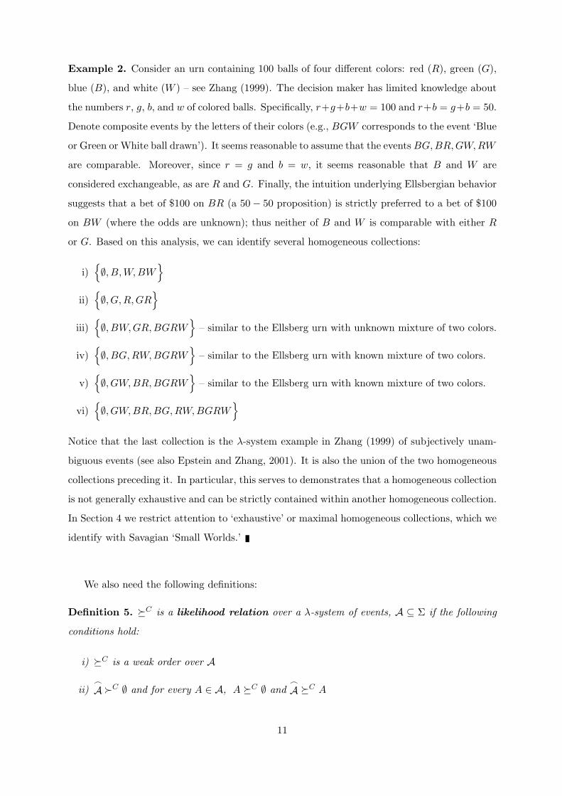
Example 2. Consider an urn containing 100 balls of four different colors: red (R), green (G),

blue (B), and white (W ) – see Zhang (1999). The decision maker has limited knowledge about

the numbers r, g, b, and w of colored balls. Specifically, r+g+b+w = 100 and r+b = g+b = 50.

Denote composite events by the letters of their colors (e.g., BGW corresponds to the event ‘Blue

or Green or White ball drawn’). It seems reasonable to assume that the events BG,BR, GW,RW

are comparable. Moreover, since r = g and b = w, it seems reasonable that B and W are

considered exchangeable, as are R and G. Finally, the intuition underlying Ellsbergian behavior

suggests that a bet of $100 on BR (a 50− 50 proposition) is strictly preferred to a bet of $100

on BW (where the odds are unknown); thus neither of B and W is comparable with either R

or G. Based on this analysis, we can identify several homogeneous collections:

i)∅, B, W, BW

ii)

∅, G,R, GR

iii)

∅, BW,GR,BGRW

– similar to the Ellsberg urn with unknown mixture of two colors.

iv)∅, BG, RW,BGRW

– similar to the Ellsberg urn with known mixture of two colors.

v)∅, GW, BR,BGRW

– similar to the Ellsberg urn with known mixture of two colors.

vi)∅, GW, BR,BG,RW, BGRW

Notice that the last collection is the λ-system example in Zhang (1999) of subjectively unam-

biguous events (see also Epstein and Zhang, 2001). It is also the union of the two homogeneous

collections preceding it. In particular, this serves to demonstrates that a homogeneous collection

is not generally exhaustive and can be strictly contained within another homogeneous collection.

In Section 4 we restrict attention to ‘exhaustive’ or maximal homogeneous collections, which we

identify with Savagian ‘Small Worlds.’

We also need the following definitions:

Definition 5. C is a likelihood relation over a λ-system of events, A ⊆ Σ if the following

conditions hold:

i) C is a weak order over A

ii)_AC ∅ and for every A ∈ A, A C ∅ and

_A C A

11

iii) for every A,B, C ∈ A such that C ∩ (A ∪B) = ∅, A C B ⇔ A ∪ C C B ∪ C

Note that the last requirement is satisfied by the definition of C .

Definition 6. µ is an agreeing probability measure for C over a λ-system, A ⊆ Σ, if it is

a probability measure over A and for every A,B ∈ A, A C (C)B ⇔ µ(A) ≥ (>)µ(B).

Finally, we require to be ‘bounded’:

Axiom 3 (Weak Event Archimedean Property). If ei∞i=0 ⊆ Σ is a sequence of disjoint

events with ei ≈ ei+1 for every i = 0, ..., then e0 is null.

Axiom 3 prevents pathological situations in which Σ contains an infinite number of disjoint

and ‘equally likely’ non-null events.

3. Probabilistic Sophistication Without Monotonicity

While homogeneity may be appealing, on its own it is not sufficient for the existence of a

likelihood relation, let alone a unique agreeing probability measure. As we discuss later, Savage’s

P3 in conjunction with P1, P5, and the Event Archimedean Property is sufficient to ensure the

existence of a unique agreeing probability measure that coincides with C when it is complete

over Σ.9 Grant (1995), however, convincingly argues that an insistence on Savage’s P3 may

descriptively exclude some decision makers that rely on subjective probabilities for decision

making. In particular, he cites the example of a mother that strictly prefers tossing a coin to

determine how an indivisible good is to be distributed among her two children. Another example

noted by Grant (1995) is that of induced preferences, which are quasi-convex.

In addition, mean-variance preferences commonly used in financial economics and manage-

ment science, are probabilistically sophisticated by definition, yet violate both P3 and P4 (as

well as both of Grant’s (1995) weakening of P3 and Machina and Schmeidler’s (1992) P4∗).10

In order that ≈ can be interpreted as an ‘equal likelihood’ relation between events in a homo-

geneous collection, we need to impose additional structure such that ≈ is transitive, at least

when restricted to the collection. It is desirable that any such structure be as parsimonious

as possible if one is to develop a better understanding of deviations from global probabilistic

sophistication. The following example provides some insight into both the limitations of an9 Savage’s P3 states that for any non-null event, E ⊆ Ω, act f ∈ F and any x, y ∈ X, x y ⇔ xEf yEf .

10 Savage’s P4 states that for any events E, E′ ∈ Σ and x∗, x∗, y∗, y∗ ∈ X with x∗ x∗, y∗ y∗, x∗Ex∗

x∗E′x∗ implies y∗Ey∗ y∗E′y∗. Machina and Schmeidler’s (1992) more restrictive P4∗ requires that for anyf, g ∈ F and whenever E ∩ E′ = ∅, x∗Ex∗E

′f x∗E′x∗Ef implies y∗Ey∗E′g y∗E′y∗Eg.

12

exchangeability based approach to probabilistic sophistication and the nature of the additional

assumptions that are called for to ensure probabilistic sophistication.

Example 3. Consider the ‘mother’ example supplied by Grant (1995) and mentioned above.

If there are only two outcomes in the world of the decision maker - namely, receipt of the

indivisible good by Child 1 or by Child 2 - then a plausible representation for the mother’s

preferences is the utility function U(p) = p(1 − p), where p is the probability that Child 1

receives the indivisible good and is subjectively generated by some device deemed by the mother

to be uniform. According to the definition of exchangeable events, any event with probability

p ∈ [0, 0.5] is exchangeable with its complement.

In the example, ≈ fails to deliver a notion of likelihood because given three disjoint events,

E,E′ and A such that µ(E) = µ(E′) = 0.4 and µ(A) = 0.2, the mother’s preference behavior

leads to the conclusion that E ≈ E′ while E ∪ A ≈ E′. To ensure an ‘equal likelihood’ inter-

pretation for ≈, a natural condition is to assume that whenever two events are exchangeable,

adding a disjoint non-null event to one of them makes the combined event more likely:

Axiom 4 (Weak Event Non-satiation). For any disjoint E,A, E′ ∈ Σ, if E ≈ E′ and A is

non-null, then E ∪A C E′.

Notice that Axiom 4 rules out the behavior in Example 3. To further motivate and under-

stand Axiom 4 consider three equivalent forms:

Proposition 1. Given P1, the following are equivalent:

i) Axiom 4

ii) Let E,A, E′ ∈ Σ with A both non-null and disjoint from E. Then E C E′ implies

E ∪A C E′.

iii) For any E,E′ ∈ Σ, E C E′ whenever E C E′ and there is some comparison event,

e ⊆ E \ E′, such that E \ (e ∪ E′) is not null.

iv) Let E,A, E′ ∈ Σ be disjoint, E and E′ be exchangeable, and A be non-null. Then for

every e′ ⊆ E′ there are outcomes, x, x′ ∈ X and act f ∈ F such that x(A ∪ E)x′e′f 6∼

x′(A ∪ E)xe′f .

According to Part (ii) of the proposition, Axiom 4 can be equivalently stated using a C

relation between E and E′. Part (iii) of the proposition can be trivially asserted for disjoint

events as E C E′ if and only if whenever e ⊂ E is a comparison event, then E\e is not null – an

13

intuitive property of any likelihood relation that can be represented by an agreeing probability

measure. The fourth part of Proposition 1 is an equivalent way of asserting Axiom 4 only in

terms of the preferences of the decision maker. It can be understood as a requirement of richness

on the outcome space: X must contain payoffs that can ‘discriminate’ between events that are

strictly ordered in terms of likelihood, so that such events are not deemed exchangeable. Note

that this is not the case in the coin tossing mother example. On the other hand, if the mother

can conceive of access to an additional divisible good, say chocolate that she can distribute

among her two children, it will likely no longer be the case that any event is exchangeable with

its complement; for instance, if E is a probability 0.6 event, then it is reasonable to suppose

that the mother is not indifferent between giving each child a piece of chocolate if E is realized

and nothing otherwise, versus giving each child a piece of chocolate if the complement of E is

realized and nothing otherwise.

The Axiom is also sufficient (though not necessary) for another intuitively sensible implica-

tion:

E′ ∼C E ⇔ E ≈ E′.

The next result establishes that Axiom 4 is necessary for any exchangeability based likelihood

relation in which non-null sets are strictly more likely than the empty set. In particular, Ax-

iom 4 is a minimal requirement for any sensible theory of probabilistic sophistication in which

exchangeable events are equally likely.

Lemma 2. Assume P1 and that is a likelihood relation over Σ with (i) a symmetric part that

agrees with ≈ on disjoint sets, and (ii) A ∅ for all non-null A ∈ Σ. Then for any disjoint

E,E′, A ∈ Σ such that A is not null, E ≈ E′ implies that E ∪A E′.

Proof : Assume that E,E′, A ∈ Σ are disjoint, A is not null, and E ≈ E′ (meaning that

E ∼ E′). Note that A ∅ ⇔ E ∪ A E. Transitivity of implies that E ∪ A E′.

If E ∪ A ∼ E′ then E ∪ A ∼ E. In particular, the cancellation property (iii) of a likelihood

relation means that A ∼ ∅ – a contradiction. Thus E ∪A E′.

Our first major result delivers global probabilistic sophistication as a result of P1, P5, Axiom

3, Axiom 4 and the assumption that every event is comparable to every other event (i.e., C is

complete).

Theorem 1. Assume P1. Then C is complete and Axioms P5, 3 & 4 are satisfied if and only

if there exists a unique probability measure, µ, representing C such that any two events with

14

the same measure are exchangeable, and the decision maker is indifferent between any two acts

that induce the same lottery with respect to µ. Moreover, if Σ is atomless then the measure is

convex-valued, otherwise Σ is atomic with each atom having the same mass.

Theorem 1 requires very weak conditions on preference. In particular, it does not require

continuity of preferences. As an example, consider Ω = [0, 1] with Σ the usual Borel σ-algebra.

Let X = [0, 1] and assume that the decision maker ranks any simple act according to the

expected value of the lottery it induces (with respect to the uniform measure on [0, 1]), and

if two lotteries have the same mean the decision maker prefers the one with smaller variance.

It should be clear that the decision maker’s preferences are lexicographic and therefore not

continuous. Since acts are evaluated based on the probability measure they induce, the decision

maker is probabilistically sophisticated and her preferences satisfy the hypothesis of Theorem 1.

Theorem 1 also requires little if any monotonicity of preferences: assuming a sufficiently rich

outcome space, both the coin-tossing mother example and induced preferences can be accom-

modated simultaneously, as can mean-variance, trimmed mean, Winsorized mean, and certain

lexicographic preferences.11 We will shortly return to discussing this result in the context of

existing literature.

It is useful to investigate conditions that ensure the existence of a continuous utility rep-

resentation over the act-induced lottery space. Other approaches (e.g., Savage, 1954; Machina

and Schmeidler, 1992; Grant, 1995; Epstein and Zhang, 2001) impose variants of Savage’s P6,12

and rely on some form of monotonicity to establish the continuity properties of a utility repre-

sentation. The relative absence of any notion of monotonicity in our approach prevents us from

being able to follow this path; P6 is not enough to establish order denseness – f g implies the

existence of h ∈ F such that f h g – necessary for the existence of a utility representation.13

Instead, we adopt a notion of continuity that is more appropriate for our setting. Beforehand,

define aimi=1 to be a uniform m-partition of E ∈ Σ whenever the ai’s are disjoint,

⋃mi=1 ai = E,

and ai ≈ aj for any i, j = 1, ...,m. Furthermore, for any partition of Ω, eiki=1 ⊂ Σ and

f1, ..., fk ∈ F , let (fi, ei)k denote the act that pays fi in event ei (for i = 1, ..., k). Note that

g E (fi, ei)k is therefore the act that pays g(ω) if ω ∈ E and fi(ω) if ω ∈ ei \E (for i = 1, ..., k).

Assuming X is a compact metric space, we write fn → f , for f = (xi, ei)k, whenever

fn = fn En (fi,n, ei)k for each n, with maxx∈fi,n(ei)

||x − xi|| → 0 for every i = 1, ..., k, and for

11For the α-Winsorized mean, instead of trimming, outliers are concentrated at the α and 1− α percentiles.12 Savage’s P6 requires that whenever f g, then for any x ∈ X there is a sufficiently fine finite partition of

Ω, say Eini=1 ⊂ Σ, such that xEif g and f xEig for every i = 1...n.

13This condition, also known as ‘dense ordering’, guarantees a functional representation. The latter need notbe continuous. See Kreps (1988) for details.

15

arbitrary integer m > 0, there exists a uniform m-partition of some non-null E, say aimi=1, and

N > 0 such that for every n > N En ⊆ a1. The continuity axiom can now be stated in terms of

‘convergence in acts’:

Axiom 5 (Continuity). X is a compact metric space, and whenever fn → f , gn → g,

and fn gn for each n, it must be that f g.

As might be expected, adding this axiom leads to a continuous utility representation over

induced lotteries.

Theorem 2. Axioms P1, P5, 3-5 are satisfied and C is complete if and only if for every

f, g ∈ F

f g ⇔ U(Ff ) ≥ U(Fg)

where for any h ∈ F , Fh is the lottery induced by h from µ, characterized in Theorem 1, and

U : Fh|h ∈ F 7→ R is non-constant and continuous in the topology of weak convergence.

An analogous theorem can also be derived when X is only a separable metric space, but the

definition of ‘act convergence’ needs to be appropriately modified to reflect the possibility of

outcomes becoming unbounded as their supports approach a null event.

Homogeneous Collections

The examples discussed in the Introduction provide vivid instances of deviation from global

probabilistic sophistication. Given our much weaker setup, departures from probabilistic think-

ing can be traced to violations of P1, P5, Axiom 3, Axiom 4, or the assumption that C is

complete (i.e., any two events are comparable). Despite the example of the coin-tossing mother

(in a highly restricted outcome space), it seems most fruitful to explore deviations from the

last assumption. As motivated in the Introduction, there are decision making situations where

completeness of C over Σ is not a compelling assumption. In such cases C is not guaranteed

to be transitive even if Axioms 3 and 4 hold (see Example 1). One may hope, however, that

when restricted to a homogeneous collection C can be shown to be a likelihood relation if

satisfies P1, P5 and Axioms 3 and 4. Examination of the proof of Theorem 1 confirms that this is

generally true whenever the homogeneous collection is a σ-algebra. However, without imposing

an algebraic structure on a homogeneous collection we are unable to show that Axioms 3 and

4 are sufficient for transitivity of C . Consider, instead, the following strengthenings of these

conditions:

16

Axiom 3′ (Event Archimedean Property). Let en, dn∞1 be a collection of disjoint events

in Σ and set d0 = ∅. If dn−1 ∪ en ≈ en+1 ∪ dn+1 for every n ≥ 1, then e1 ∪ d1 is null.

To motivate Axiom 3′, consider that if dn−1 ∪ en ≈ en+1 ∪ dn+1 for every n ≥ 1, then by

adding dn to each side of the relation one intuitively obtains that e1∪d1 is ‘as likely as’ d1∪e2∪d2,

which is in turn ‘as likely as’ d2 ∪ e3 ∪ d3, which is in turn as likely as d3 ∪ e4 ∪ d4, and so on.

If the relation ‘as likely as’ is transitive, the construction leads to an infinite number of disjoint

and equally likely events: e1 ∪ d1, d2 ∪ e3 ∪ d3, d4 ∪ e5 ∪ d5, etc. Thus to prevent pathological

situations in which Σ contains an infinite number of disjoint and ‘equally likely’ non-null events,

we require that such a construction is possible only if e1∪d1 is null. Note that the axiom asserts

this property even if the relation ‘as likely as’ is not transitive; moreover, setting dn = ∅ for

every n > 0 implies Axiom 3.

Consider also the following strengthening of Axiom 4,

Axiom 4′ (Event Non-Satiation). For any disjoint E,E′, A ∈ Σ, if x(E ∪ A)x′E′f ∼

xEx′(E′ ∪A)f for every x, x′ ∈ X and f ∈ F then A is null.

In particular:

Lemma 3. Given P1, Axiom 4′ implies Axiom 4.

Notice that while the converse of Lemma 3 is not true, there is some similarity between part

(iv) of Proposition 1 and event non-satiation.

In this slightly richer setting, we can extend our results to homogeneous collections (λ-

systems) that are closed under countable unions.

Theorem 3. Assume P1, Axiom 3′, Axiom 4′, and that A ⊆ Σ is closed under countable disjoint

unions and contains at least one non-null event. Then A is homogeneous if and only if C is

a likelihood relation over A with a unique agreeing probability measure such that any two events

with the same measure are exchangeable. If A is atomless then the measure is convex-valued,

otherwise A is atomic with each atom having the same mass.

Note that the representation of C by a unique probability measure applies to any homoge-

neous collection, including homogeneous ‘sub-collections’ of homogeneous collections. Clearly,

investigating the latter is redundant. Instead, we are led to the following:

Definition 7 (Domains). D ⊆ Σ is a small world event domain if it is a homogeneous

subset of Σ with the following properties:

17

i) D contains at least one non-null event.

ii) If A ⊆ Σ is a non-empty collection of events and A ∪D is homogeneous, then A ⊆ D.

iii) D is closed under countable disjoint unions.

For brevity, we will henceforth refer to any small world event domain simply as a ‘domain’.

The first condition is akin to ‘non-triviality’. The second property, a maximality condition,

guarantees that the domain is a ‘maximal’ homogeneous structure and justifies the association

of D with the notion of a Savagian ‘small world’. The third condition is technical and ensures

that Theorem 3 delivers probabilistic sophistication on domains. Note the following properties:

(i) If Σ is a domain then it is the only domain and under the hypothesis of Theorem 1 the

decision maker is probabilistically sophisticated, (ii) if Σ does not contain domains, then no two

non-null events are exchangeable.

Denote by µD the unique measure representing C on a domain, D, satisfying the hypothesis

of Theorem 3. One would like to conclude from Theorem 3 that the decision maker is indifferent

between any two acts, say f and f ′, that are identical outside a domain, while inducing the

same lottery on the domain. Unfortunately, barring other conditions, this is not generally true

unless D is a σ-algebra, or the identical lotteries in question are binary. This situation is not

unique to our approach; in both Epstein and Zhang (2001) and Kopylov (2002) monotonicity is

crucial to demonstrate indifference between such a pair, f and f ′. In place of a monotonicity

condition, consider the following criterion:

Axiom 6. Let eimi=1, e′im

i=1 ⊂ Σ be uniform m-partitions of E ∈ Σ such that ei ∼C e′j for

any i, j ∈ 1, ...,m. Then for any f ∈ F , ximi=1 and permutation σ : 1, ...,m 7→ 1, ...,m,

x1e1...xmemf ∼ xσ(1)e′1...xσ(m)e

′mf .

Consider that exchangeability of two events amounts to indifference between permutations

of payoffs among the events. Axiom 6 can be interpreted to say that if two different partitions

of the same event are ‘exchangeable’ (in the sense of ∼C) event by event, then the two partitions

are ‘exchangeable’.

Let D be a domain and denote by FD the set of acts adapted to D. Given the unique

measure, µD over D from Theorem 3, the portion of each act in FD that is adapted to D induces

a distribution. Let ∆µ(FD) be the set of all such distributions induced by µD and FD. If

f ∈ FD then the conditional probability distribution associated with it through µ is denoted as

Ff |D. Finally, we identify the set of deterministic lotteries, δx ∈ ∆µ(FD) | x ∈ X, with X.

18

Theorem 4. Suppose P1 and Axioms 3′, 4′, 5 and 6 hold, and D ⊆ Σ is a domain. Then

there exists UD : ∆µ(FD) × F 7→ R, continuous in its first argument (in the topology of weak

convergence), such that µD is characterized in Theorem 3, and for every f, g ∈ F adapted to D

and h ∈ F :f

_D h g

_D h ⇔ UD(Ff |D, h) > UD(Fg|D, h).

The ‘representation’ in Theorem 4 is not fully satisfactory since it does not generally allow

one to pin down risk preferences over a domain unless the domain envelope is the entire state

space. Section 4 addresses this by specializing to the case where UD(·, h) is independent of h for

any D. In the remainder of this section we continue to relate our approach to the literature on

probabilistic sophistication. In one subsection we compare our characterization of probabilistic

sophistication (via Theorem 1) to that of Machina and Schmeidler (1992), and Grant (1995).

In the next, we discuss how exchangeability based probabilistic sophistication is related to the

literature on state dependent preferences. The last subsection discusses Theorem 3 in the context

of the literature on non-global probabilistic sophistication.

3.1. Homogeneity, Monotonicity, and Probabilistic Sophistication

Machina and Schmeidler (1992) show that P1, P3, P4∗, P5 and P6 are necessary and suffi-

cient for the existence of a continuous probabilistically sophisticated utility representation of

that agrees with first degree stochastic dominance (see Footnotes 9, 10 and 12 for definitions).

Grant (1995) weakens P3 to either one of two variants: conditional upper (or lower) eventwise

monotonicity (P3CU or P3CL). These state that for any x, y ∈ X, h ∈ F and disjoint non-null

E,E′ ∈ Σ,

P3CU : x(E ∪ E′)f y(E ∪ E′)f ⇒ xEyE′f y(E ∪ E′)f

P3CL: x(E ∪ E′)f y(E ∪ E′)f ⇒ x(E ∪ E′)f xEyE′f

Grant also uses a modified form of P4 stating that for all w, x, y, z ∈ X, f, g ∈ F , and disjoint

E,E′ ∈ Σ:

P4CE : x(E ∪ E′)f xEyE′f ∼ yExE′f y(E ∪ E′)f ⇒ wEzE′g ∼ zEwE′g

In the language of this paper, Grant’s P4CE supplies a sufficient condition for E and E′ to be

exchangeable. Assuming P1, P4CE , P5, a slightly strengthened form of P6, and one of P3CU or

P3CL, Grant (1995) shows the existence of a probabilistically sophisticated representation with

19

either quasi-convex or quasi-concave upper contour sets in the space of probability distributions.

Our purpose in this section is to compare the existing approaches to probabilistic sophis-

tication with ours. We begin with the Machina and Schmeidler (1992) axiomatization. Note

first that P4∗ ensures that their axioms lead to a unique convex valued probability measure

where the measures of two events coincide if and only if the events are exchangeable. Thus their

axioms imply that Σ is homogeneous (i.e., all events are mutually comparable). It is also easy to

show that monotonicity (i.e., P3) implies weak event non-satiation. One can therefore interpret

that, in establishing global probabilistic sophistication in Theorem 1, we weaken the Machina

and Schmeidler axioms as follows: P3 → Axiom 4, P4 → homogeneity of Σ, and P6 → Axiom

3. Thus aside from monotonicity considerations, our assumptions substantively weaken those of

Savage (1954) or Machina and Schmeidler (1992). Moreover, consider the following result:

Proposition 2. Assume P1, Savage’s P3, and that Σ is homogeneous. Then for any x∗, x∗ ∈ X

with x∗ x∗, disjoint E,E′ ∈ Σ, and f ∈ F , x∗Ex∗E′f x∗E′x∗Ef ⇔ E C E′, and the

latter relation is strict if and only if E C E′.

The proposition establishes two things: given a weak ordering satisfying P3, Machina and

Schmeidler’s P4∗ is an implication of the homogeneity of Σ; moreover, C is, in this case,

the comparative likelihood relation represented in their probabilistically sophisticated setting.

In other words, to arrive at their representation theorem one need only add P3 to the list of

conditions in our Theorem 2.

As stated, our axioms do not encompass those of Grant (1995) whose approach, in particular,

can accommodate Example 3. On the other hand, Grant’s axioms are more demanding in the

sense that taken as a whole they imply homogeneity of Σ, require a form of continuity that is not

needed in Theorem 1, and rule out many probabilistically sophisticated functional forms that

are behaviorally reasonable and admissible under our axioms. Consider the following result:

Proposition 3. Assume P1 and that for every non-null A ∈ Σ, f ∈ F , there exist x, x′ ∈ X

such that xAf f x′Af . Then either one of P3CU or P3CL implies Axiom 4.

The condition “for every non-null A ∈ Σ, f ∈ F there exist x, x′ ∈ X such that xAf f

x′Af” is a form of non-satiation in outcomes: there is always something sufficiently good (resp.

bad) that the decision maker is happy (resp. reluctant) to substitute for the payoff scheme

determined by f on A. It can therefore be viewed as a ‘richness’ assumption on both and

the outcome set, X. Indeed, it is a challenge to find an intuitively behavioral example in a

state independent setting where the state space cannot be so ‘enriched’. To further emphasize

20

the importance of ‘enriching’ the outcome space, we note that whenever X contains only two

outcomes, Σ is non-atomic, and can be represented via a continuous and probabilistically

sophisticated utility function, Axiom 4 is satisfied if and only if the representation is monotonic

in the sense of P3.14

Proposition 3 establishes that in the presence of a ‘rich’ outcome space, either one of Grant’s

P3CU and P3CL implies Axiom 4. Moreover, since in this case Grant’s unique measure rep-

resenting probabilistic sophistication agrees with C , his axioms (taken together) imply both

homogeneity of Σ and Axiom 3. In other words, probabilistically sophisticated preferences that

satisfy Grant’s axioms also satisfy ours provided that the outcome space is sufficiently rich to

ensure that Axiom 4 is also satisfied. We note once more that the mother example in which

there are only two equally ranked outcomes (i.e., Example 3) does not satisfy Axiom 4 but does

satisfy Grant’s conditions. However, if there are at least two outcomes such that the mother

strictly prefers placing more probability on one versus the other in almost every binary lottery,

then Axiom 4′, and thus Axiom 4, is satisfied.

Theorem 1 applies to many instances in which P3CU and P3CL are violated, including but not

limited to cases where upper contour sets of preferences over distributions are not always quasi-

concave or quasi-convex. Moreover, in addition to violating P3 and its variants, some common

choice models, such as mean-variance preferences, also violate P4 and its variants while leaving

the homogeneity of Σ intact. However, there is one other advantage to an exchangeability

based approach to probabilistic sophistication beyond the fact that it encompasses other known

models (given a ‘richness’ assumption). As demonstrated with Theorem 4, our exchangeability

based approach lends itself particularly well to studying deviations from global probabilistic

sophistication, and does not confound such deviations with other behavioral considerations such

as monotonicity or continuity.

In summary, there is an analogy between the standard axioms required for probabilistic

sophistication and ours. All approaches share P1 and some form of P5. We weaken the standard

continuity axiom (e.g., P6) to the event Archimedean property, and weaken the P4 variants to

the assumption that all events are comparable. Monotonicity is replaced by Axiom 4. Grant’s

P3CU and P3CL, however, are not strictly contained within our set of axioms, unless the outcome

space is enriched so as to satisfy the hypothesis of Proposition 3.14We thank I. Gilboa for pointing this out.

21

3.2. State Dependence

One often interprets Savage’s P3 and P4 to jointly assert a separation between tastes and beliefs,

or ‘state independence’ (see, for example, Sarin and Wakker, 2000). Theorem 1 and Theorem

2 are state independent in the sense that the decision maker to which these theorems apply

only cares about the likelihood of an event and not its identity. The axioms leading to these

two results are weaker than P3 and P4, thus prompting the obvious question: which of our

assumptions embodies the sense of ‘state independence’? A possible answer is the same one we

provided for ruling out Ellsbergian or source dependent behavior; i.e., C is complete, and thus

all events are comparable. For instance, in the Aumann-Savage correspondence documented in

Dreze (1987), two equally likely events – ‘rain in Chicago’ and ‘no-rain in Chicago’ – are not

exchangeable with respect to the outcomes ‘trip to Chicago with umbrella’ and ‘trip to Chicago

without an umbrella’. While they may well be exchangeable with respect to other outcomes (e.g.,

trip to San Francisco with, versus without, an umbrella), the two events are not exchangeable

with respect to the ‘Chicago plus/minus umbrella’ payoffs even though they are associated with

unique probabilities. In particular, the two events are not comparable via C .

Informally, one is able to distinguish between incompleteness of C due to Ellsbergian or

similar behavior, versus the type of state dependence outlined above. In this subsection we

explore the extent to which one can formally distinguish the two types of incompleteness. In

so doing we sketch a basis for understanding state dependence and ‘small world’ attitudes

vis-a-vis exchangeability. Rather than provide a comprehensive treatment of the subject, our

goal is to outline how an exchangeability based approach may contribute to the literature on

state dependence whose primary focus concerns global probabilistic sophistication based on the

expected utility specification (see Karni, Schmeidler and Vind, 1983; Dreze, 1987; Karni, 1993;

and Karni, 2003).

In the Aumann example, one can conceivably discern the probabilistic sophistication of the

decision maker by restricting attention to acts whose payoffs are not related to the identity of

events. For example, in assessing probabilistic sophistication, one could focus on the behavior of

the decision maker with respect to pure monetary outcomes. Note that in order to accommodate

the coin-tossing mother from Example 3 we require the outcome space to be enriched beyond two

outcomes, while to accommodate probabilistic sophistication in the presence of state dependence

we require precisely the opposite. To proceed formally, let Y correspond to the preference

relation obtained by restricting the set of outcomes to Y ⊆ X . Define ≈Y and CY similarly,

then

22

Definition 8 (State Independent Preferences). is state independent when CY =C

Y ′

for every pair of outcome sets, Y, Y ′ ⊆ X, such that Y and Y ′ satisfy P5 and Axiom 4′.

A preference relation is state independent when essentially every outcome set can be used

to elicit subjective probabilities within a domain. We require P5 and Axiom 4′ so as to exclude

scenarios such as Example 3 which seems intuitively state independent. We caution the reader

that our definition does not fully capture the intuition behind ‘state independence’. For instance,

in the Aumann-Savage example one might consider a very simple outcome space, spanning ‘trip

to Chicago with x’, where x ∈ X = expensive umbrella, average umbrella, cheap umbrella, in

which intuitively there appears to be state dependence. However, since the ‘connection’ between

the outcomes and the states is uniform across outcomes, is ‘state independent’ according to

our definition. Notice that this mis-labeling is shared by other definitions of state dependence,

such as the requirement that satisfies P3 and P4. In applications, however, our notion of state

independence seems to accord with intuition. Moreover, we take as uncontentious the claim that

if is not ‘state independent’ according to our definition, then it is state dependent. In any

case, if is state independent, then any structure characterizing C – in particular, deviations

from global probabilistic sophistication – can only be due to ‘small worlds’ behavior. Thus, at

least in this case, we can identify the source of incompleteness of C .

If is state dependent, the natural question is how, if possible, can one deduce a state

independent structure for C and the consequent ‘small worlds’ beliefs (i.e., Theorem 3)? To

formally answer this, let R denote the set of all restricted outcome relations such that Y ∈ R

implies Y satisfies P5 and Axiom 4′, and is itself a state independent preference relation in

the sense of Definition 8. For instance, in the Aumann example, while may not be state

independent, its restriction to monetary outcomes might be.

Definition 9 (State Independent ‘Beliefs’). CR is termed a state independent event

comparability relation on Σ if R is not empty and for any Y ∈ R, CY =C

R.

Thus as long as every state independent restriction of induces the same comparability

relation, this relation, denoted as CR, can be said to be itself state independent. Note, first of

all, that for any E,E′ ∈ Σ and Y ⊆ X, E C E′ ⇒ E CY E′. Thus, since C is generally a

partial order, CR, if it exists, can be seen as a ‘more complete’ extension (or superset) of C .

Thus existence of CR allows one to identify the component of incompleteness of C due to state

dependence as the set difference between CR and C . Moreover, if C

R exists and is complete

then Theorem 3 implies global probabilistic sophistication in the presence of state dependence.

23

In contrast with existing literature on state dependent preferences, this characterization does

not hinge on an expected utility framework.

Some forms of state dependence, for instance situations involving moral hazard (see Karni,

2003), may not allow for the existence of the relation, CR. Thus, while it complements the

literature on probabilistic sophistication with state dependence, the approach sketched above is

not comprehensive. We leave a more thorough investigation to future research.

3.3. Relation to Subjectively Unambiguous Events

One focus of the current literature on decision making under uncertainty is to distinguish events

on which a decision maker is globally probabilistically sophisticated, from those on which the

decision maker’s likelihood relation does not admit a probabilistic representation. The former are

often called ‘unambiguous’ while the latter are termed ‘ambiguous’ events. In this subsection we

relate this literature to our approach based on domains. It is worth emphasizing that examples

abound in which the noncomparability of events does not stem from the presence of ambiguity

in any particular way. Thus prima facie a focus on domains differs in scope and purpose from

the literature on ambiguity.

Epstein and Zhang (2001) define unambiguous events (see below) using Savage-like primi-

tives; Ghirardato and Marinacci (2002) rely on degrees of what they term ambiguity aversion to

identify unambiguous events; Nehring (2001) and Ghirardato, Marinacci and Maccheroni (2003)

define an event to be unambiguous if the event’s probability is the same under every measure

in an endogenously determined set of measures representing an incomplete comparative likeli-

hood relation;15 Klibanoff, Marinacci and Mukerji (2002) define ambiguous events by relying on

benchmark lotteries with respect to an ‘objective’ randomization device (or other appropriate

enrichment of the state space). These references do not generally agree on the ambiguity of

specific events as inferred from the decision maker’s choice behavior.

All the definitions discussed above have their compelling aspects. The definition given by

Epstein and Zhang (2001), which applies to preferences satisfying Savage’s P3, appears to be

the least dependent on imposing additional structure on . The definitions offered by Nehring

(2001) and Ghirardato, Marinacci and Maccheroni (2003) are also quite general but, besides a

version of Savage’s P4, require additional global structure over preferences to ensure the existence

of a Bewley-like partial qualitative likelihood relation. Ghirardato and Marinacci’s (2002) can15Siniscalchi (2003) notes that multiple prior models can also be characterized by a unique set of measures, each

of which provides a subjective expected utility representation when is restricted to a particular convex set ofacts that contains all the constant acts. While one can view this as ‘probabilistic sophistication’ over domains ofacts, this approach does not share our aim of characterizing probabilistic attitudes towards collections of events.

24

be interpreted as specializing to a particular class of preferences which reduce to expected utility

in the absence of ambiguity. Klibanoff, Marinacci and Mukerji (2002) arguably make the most

imposing requirements over preferences, but their definition is remarkably clean: by a priori

enriching their state space with an ‘objective’ randomization device, they can compare risk

preferences over objective lotteries and preferences over Savage acts. In such a comparison

between a binary bet on an event versus an objective lottery, deviation from P4 implies that

the event is ambiguous.

A natural question is what overlap, if any, exists between event classification through domains

and classification into ‘ambiguous’ versus ‘unambiguous’ events. We focus on the definition

supplied by Epstein and Zhang (2001). Examples to differentiate domains from the other theories

are straightforward to construct.

Epstein and Zhang (2001) define subjectively unambiguous events as follows: E ∈ Σ is EZ-

unambiguous if the following two conditions are satisfied (i) for any x, x′, z, z′ ∈ X, f ∈ F

and A,B ∈ Σ such that A,B ⊆ Ec and A ∩B = ∅,

zExAx′Bf zEx′AxBf ⇒ z′ExAx′Bf z′Ex′AxBf.

and, (ii) condition (i) holds if E is everywhere replaced by Ec. It is straight forward to check

that in all the urn examples considered so far EZ-unambiguous events constitute domains or

unions of domains. In particular, each unambiguous event is comparable to every other. An

obvious question is whether ‘EZ-unambiguity’ implies comparability more generally. The answer

turns out to be no, as the following example illustrates.

Example 4. Consider the four-color urn with the only information about the color combinations

being that g > r > w = b. Assume a monotonic utility representation for given by

V (xB, xW , xR, xG) = xB + xW + xR + xG + (xG + 1)(xR + 2)

with xB, xW , xR, xG ∈ R+. Moreover, the event GB is unambiguous. To see this, consider that

fixing the payoff on GB, the decision maker’s attitudes towards permuting payoffs on R and W

are summarized by

V (xGB, xW , xR, xGB) ≥ V (xGB, xR, xW , xGB) ⇔ (xGB + 1)(xR − xW ) ≥ 0 ⇔ (xR − xW ) ≥ 0

and are therefore independent of the fixed payoff on GB. Thus the first requirement of ‘EZ-

25

unambiguity’ is satisfied. It is easy to check that the complementary condition holds as well.

Analogously,∅, GB, RW,GW,RB, GBRW

is the λ-system of EZ-unambiguous events. How-

ever, not every EZ-unambiguous event is comparable to every other. In particular, GB is not

comparable to RW (since G and R are not exchangeable).

In the above example, note that the decision maker’s preferences satisfy Savage’s P3 and

even P4 restricted to EZ-unambiguous events.

Another natural question is whether the domain language can be used to characterize the dis-

tinction between ‘ambiguous’ and ‘unambiguous’ events. We observe instead that a preference-

based definition of ‘unambiguous’ events may not always accord with intuition. For instance,

consider the two-urn Ellsberg example discussed in the introduction and two decision makers.

The first exhibits the conventional preference pattern of preferring to bet on the known urn

while the other exhibits the opposite pattern of preferring to bet on the unknown urn. How is

an observer who does not know which urn is ‘ambiguous’ or which decision maker is ‘ambiguity

averse’ to tell both the difference between the urns and the difference between the two decision

makers? From the perspective of the observer there is sufficient symmetry to prevent such in-

ference – doing so requires information external to the primitives at hand. In particular, any

definition that identifies a domain of events as ambiguous in the case of one decision maker will

simultaneously identify it as unambiguous in the case of the other decision maker. This difficulty

also seems inherent to the definitions in Epstein and Zhang (2001), Nehring (2001), Ghirardato

and Marinacci (2002) and Ghirardato, Marinacci and Maccheroni (2003). In other words, the

‘knowledge’ that in one urn the distribution of balls is unambiguous while it is ambiguous in the

other is exogenous and cannot be reliably inferred through observation of the decision maker’s

preferences alone. Klibanoff, Marinacci and Mukerji (2002) avoid this by explicitly incorporating

the exogenous knowledge about the known urn into the decision maker’s preferences (i.e., the

known urn is a randomization device which, by definition, receives differential treatment in the

decision maker’s preferences).

While we refrain from proposing a definition of unambiguous events, we can say (relative to

state independent outcomes) that ‘ambiguity’ corresponds to the presence of multiple domains,

or more generally, having at least two non-null events that are not comparable. Lack of com-

parability suggests that there are different sources, interpretations, or ‘issues’, in the language

of Ergin and Gul (2002), associated with the noncomparable events, and thus the presence of

ambiguity. One may hope to say something more concrete than this, but such hope may be

in vain. For instance, suppose that one were to expand the outcome space to lotteries, as in

26

the Anscomb-Aumann approach or the enriched state space approach advocated by Klibanoff,

Marinacci and Mukerji (2002). One can then define a domain to be unambiguous if risk prefer-

ences within that domain are identical to risk preferences over objective lotteries associated with

the same distribution functions. This intuition relies on the assumption that the lotteries in the

expanded outcome space are somehow unambiguous a priori. In other words, one relies on the

‘neutral-ness’ of objective lotteries. However, as will be discussed in Subsection 4.1, examples

of distinct domains over different lottery spaces are not uncommon. For example, consider the

two-urn example where the first urn contains 50 red balls and 50 black balls, while the second

urn has one red ball and one black ball. Although the proportion of balls is the same in each

urn, a decision maker may prefer to draw from the urn containing more balls, reasoning that

there will be less ‘regret’ if he is disappointed by the realized outcome (e.g., ‘Darn! I had the

winning ball in my hand!’).

4. Domains, Ellsbergian Behavior and Representations

We begin the section by discussing examples of multiple domains risks. This motivates additional

axioms relating to the structure of domains, which are necessary for characterizing domain

recursive utility for mixed acts across distinct domains.

4.1. Examples of State Independent Multiple Domains Risks

In addition to the discussion in the Introduction on choice behavior in a multiple domain context,

we illustrate here how multiple domains can arise in additional settings. We assume throughout

this subsection that preferences are state independent.

Examples involving Urns

Consider an urn containing 50 red balls (R), plus a combination of green (G) and blue (B) balls

that sum to 50. It seems reasonable that people would find B exchangeable with G and BG

exchangeable with R. In other words, there are two domains: ∅, G,B,BG, and ∅, R, BG,Ω.

Based on the possible homogeneous collections identified in Example 2, we can readily iden-

tify the following domains in the four-color urn: DBW =∅, B, W, BW

, DGR =

∅, G,R, GR

,

DBGRW =∅, BW,GR,Ω

and Dλ =

∅, GW, BR,BG,RW, Ω

.

Returning to the two-urn experiment, let Rk, Bk and Ru, Bu denote partitions of Ω

associated with drawing a single ball from each of the two Ellsberg urns: an urn containing

50 red (Rk) and 50 black (Bk) balls (the ‘k’ or known urn) and an urn containing 100 red

27

(Ru)and black (Bu) balls of unknown ratio (the ‘u’ or unknown urn). Commonly reported

behavior suggests that there is exchangeability between Rk and Gk and between Ru and Gu

but not between either Rk and Gk and either of Ru and Gu. In other words, ∅, Rk, Gk,Ω and

∅, Ru, Gu,Ω are potentially domains. By examining the decision maker’s preference for more

general acts of the form, x1 Rk ∧ Ru x2 Rk ∧ Bu x3 Bk ∧ Ru x4, one may identify additional

domains involving the conjunction of events in the two urns. We shall defer the discussion of this

question until after we have developed our results for a domain recursive utility representation

for mixed acts.

Additional Examples

The Introduction describes several multiple-domain variations of the single small world examples

due to Savage – decimal expansion of different numbers, tossing different coins, and tempera-

ture/rainfall in different cities. Introspection suggests that people may prefer to bet on the

decimal expansion of a nice number than a strange one, on one’s own coin than a coin from

someone peculiar, and on uncertainty arising from a familiar source than a foreign one. Exam-

ples of multiple domains risks can be found in daily life. For instance, giving consumers the

choice of picking their own numbers appears to be a demand-enhancing feature of state lot-

tery design. The Denesraj-Epstein (1994) study suggests that even when two sets of events are

clearly compatible with having objective probabilities, they may be differentiated by virtue of

event noncomparability in relation to certain acts. At the same time, when bets are restricted to

a single source of uncertainty the same individuals may exhibit preferences that are compatible

with probabilistic sophistication.

Since attitudes towards uncertainty within a domain are completely described by attitudes

towards risk, the presence of multiple domains enables the modeling of distinct risk preferences

within distinct domains. For instance, a decision maker may be probabilistically sophisticated

when betting only on temperature intervals in any given city. That decision maker, however,

may have different certainty equivalents for the same ‘subjective lottery’ in different cities. If

he prefers to bet on a subjective lottery in a more ‘familiar’ city, one may say that the decision

maker exhibits ‘uncertainty aversion’ towards risks arising from the less familiar city-domain.

This can be rationalized by requiring the decision maker to be more ‘risk averse’ when betting

on the unfamiliar city-domain. In the insurance context, even when hazard rates are available,

individuals appear to exercise ‘mental accounting’ when considering unusual and particularly

disastrous risks (see, Eisner and Strotz, 1961; Kunreuther et al, 1978). Our perspective may also

28

shed light on other decision situations involving uncertainty from distinct sources, e.g., domestic

(versus foreign) and local (versus national) biases of equity investors.16 In the next subsections,

we will address the question of representing the decision maker’s preference over acts that are

not adapted within a single domain.

4.2. Domain Independence and Separation

Theorem 4 concerns the representation of the decision maker’s preference among acts that are

adapted within individual domains. To further pin down possible representations over mixed

acts, a natural way to proceed is to assume, as Savage did, that decisions across small worlds

are separable. The identification of domains with Savagian small worlds leads to the following

hypothesis:

Axiom 7 (Domain Independence). X is connected, and whenever f ∈ F is adapted to events

in a domain D, there is some x ∈X such that for all g, h ∈ F , f_D g ∼ x

_D g ⇔ f

_D h ∼ x

_D h.

Domain independence is similar to Savage’s sure thing principle in that for each act adapted

to the domain, there exists a certainty equivalent over that domain that is independent of

payoffs outside the domain. While the separation among small world ‘beliefs’ is accomplished

endogenously via Theorem 3, Axiom 7 asserts an analogous separation in terms of ‘valuation’.

This assumption is not particularly normative and we do not have empirical evidence to defend

it on descriptive ground. We view it as a falsifiable hypothesis to investigate empirically. The

axiom is also instrumental in delivering a global representation of preferences exhibiting multiple

domains. Domain independence, combined with previous assumptions, delivers a well defined

(up to monotonic transformation) utility function representing the decision maker’s preferences

over each domain.

Proposition 4. If satisfies P1, P5 and Axioms 3-7, then for every domain, D, and acts

g, f ∈ F adapted to D, there exists a unique probability measure on, µ on D, and a continuous

function, WD : ∆µ(FD) 7→ R such that WD(∆µ(FD)

)= WD(X), and for every h ∈ F ,

f_D h g

_D h ⇔ WD(Ff |D) ≥ WD(Fg|D).

Proof : Suppose for some x, y ∈ X, x_D h y

_D h. Note that Axiom 7 rules out the possibility

that y_D h′ ∼ x

_D h′ for any h′ ∈ F . Assume, therefore, that y

_D h′ x

_D h′ for some h′ ∈ F .

16There is a literature (see, e.g., French and Poterba, 1991) on the ’home market bias’ phenomenon thatportfolios of equity investors are disproportionately weighted in favor of domestic stocks, relative to foreign stocks.There are further evidence (see Huberman, 2001; Coval and Moskowitz, 2001) that, within the same country, theremay also be a similar bias in favor of shares in companies that are geographically proximate. Recent theoreticalwork that attempt to rationalize this behavior in terms of uncertainty aversion includes Uppal and Wang (2002).

29

Let ei ⊂ Σ be the coarsest partition of Ω to which both x_D h and x

_D h′ are adapted. Note

that by Axiom 5 the restriction of to (xi, ei) | xi ∈ X, i = 1, ... is continuous in the sense

that upper and lower contour sets are closed. Since X is connected, one can find some h′′ ∈ F

such that y_D h′′ ∼ x

_D h′′ – a contradiction of Axiom 7. Thus it must be that x

_D h′ y

_D h′

for any h′ ∈ F , or alternatively, the ranking is independent of h′ and WD(·, h) is monotonically

equivalent to WD(·, h′).

If, according to the decision maker’s preferences, the state space is a sequence of nested

domains - much like a filtration - then the decision maker’s preference representation will emulate

that structure and appear as a recursive nesting of the domain utility functions from Proposition

4. Before proving a general result along these lines, we illustrate nested domains and the

representation implied by domain independence.

Examples

For the three-color urn containing 50 red balls plus a distribution of blue and green balls that

sum to 50, we have defined two domains: D0 = ∅, R, GB,Ω and D1 = ∅, G,B,GB. Let W0

and W1 represent risk preferences in the two domains, respectively. Note that by Proposition

4, W1(δc∗) > W1(δc∗) if and only if W0(12δc∗ + 1

2δc) > W0(12δc∗ + 1

2δc) for any c ∈ X. This

‘monotonicity’ implies that one can always find some continuous v0 : X ×R 7→ R that is strictly

increasing in its second argument, such that W0(12δxR + 1

2δc∗) > W0(12δx′R

+ 12δc∗) if and only if

v0

(xR,W1(δc∗)

)> v0

(x′R,W1(δc∗)

). In turn, identifying xR with δxR , the act (xR, xG, xB) has

a recursive utility representation

V (xR, xG, xB) = v0

(δxR ,W1(

12δxG +

12δxB )

),

where v0

(δxR ,W1(δcGB )

)= W0

(12δxR + 1

2δcGB

).

In the case of the four-color urn, one can represent a general act as (xB, xW , xR, xG) ∼

(cBW , cBW , cRG, cRG), where the indifference relation results from the domain independence

of the domains identified in Subsection 4.1. Let W1 represent over the domain generated

by B,W (and, by symmetry, R,G) in accordance with Proposition 4. Likewise, let W0

represent the risk preferences in the domain spanned by BW and RG. Then the following

recursive utility function represents :

V (xB, xW , xR, xG) = v0

(W1(

12δcB +

12δcW ),W1(

12δcR +

12δcG)

),

30

where v0

(W1(δcBW ),W1(δcRG)

)= W0

(12δcBW + 1

2δcRG

)is continuous, symmetric, and strictly

increasing in both its arguments. Note that GW,BR, BG, RW, are mutually comparable, as

are BW, RG. Moreover, events in the latter collection are not generally comparable with those

in the former unless W1 and v0 exhibit the same risk attitudes over their respective domains (in

which case the representation is globally probabilistically sophisticated).

Domain Separation

An important question to address when considering how decisions are made across domains is

how and whether domains ‘overlap’. All of the examples considered thus far have the following

structure: domain envelopes are either disjoint or ‘nested’ within a larger domain. To what

extent can this be justified more generally?

To attempt an answer to this, suppose D1 and D2 are domains, and consider any E1 ∈ D1,

such that E1 6∼C_D1 and E1∩

_D2 ∈ D2; then in all the urn examples,

_D2 ⊆

_D1. For instance,

in the four color urn example Dλ contains an event, GW , that contains the event G from DGR

– note that GR is not in Dλ – and_DGR ⊆

_Dλ. It is easy verify that the same is true for all

the other examples. To rationalize this structure more generally, set E1∩_D2= E2 ∈ D2 and let

E′1 = (E1 \E2)∪E′

2 where E′2 is any element of D2 such that E2 ∼C E′

2. It should be clear that

E1 = (E1 \ E2) ∪ E2 ∼C E′1 for every E′

1 so constructed. Thus at the level of intuition, if one

can assign a unique probability to E1 then one can assign the same probability to every event

in A ≡ E′1 = (E1 \ E2) ∪ E′

2 | E′2 ∼C E2, E

′2 ∈ D2. It therefore seems reasonable to require

that A ⊂ D1. Now, if D2 is non-atomic or generated from exchangeable atoms, then the union

of all events in E′2 | E′

2 ∼C E2, E′2 ∈ D2 is

_D2. Thus the envelope of D1 should contain

_D2.

The preceding discussion makes a compelling case for the following assumption:

Axiom 8 (Domain Separation). If D1 and D2 are domains, and for some E1 ∈ D1, where

E1 6∼C_D1 and E1∩

_D2 ∈ D2, then

_D2 ⊆

_D1.

4.3. Characterizing Domain Recursive Utility

The preceding subsection discusses examples of ‘nested domains’ with the feature that each

act can be reduced to a certainty equivalent in multiple steps akin to backward induction. In

each step an act is adapted to a set of domains whose envelopes are disjoint, so that one can

use domain independence to simplify the act further. To generalize this idea we introduce the

following:

31

Definition 10. is said to be finite domain recursive whenever it induces a sequence of

domains Dt,i, where for each t = 0, ..., T < ∞, i = 1, ..., nt with n0 = 1, nt ≤ nt+1 < ∞, and

such that the following must be satisfied:

1._D0,1= Ω.

2. For each 0 ≤ t < T − 1, 1 ≤ i ≤ nt and 1 ≤ j ≤ nt+1, either_Dt+1,j ∈ Dt,i where i is

unique in 1, ..., nt, or_Dt,i ∩

_Dt+1,j = ∅.

3. Letting Et,i ≡_Dt,i \

⋃nt+1

j=1

_Dt+1,j, if e ⊆ Et,i and e ∈ Σ, then e ∈

_Dt,i.

Diagrammatically, this structure is analogous to a T + 1-stage tree with a single base node,

and whose nodes at stage t correspond to distinct domains. Any two domains within the same

stage have disjoint envelopes, and the envelope of a domain at stage t is an event in at most

one domain at stage t − 1. The envelope of the base domain at stage 0 is the full state space.

To gain a better understanding of the last part of the definition, consider first that the event

ET,i, for i = 1, ..., nT is identically equal to_DT,i, and thus every subevent of

_DT,i is adapted

to DT,i; in other words, every act is perforce adapted to each of the DT,i’s. Now, by part (ii)

of the definition, a domain at stage t < T may contain the disjoint envelopes of some domains

from stage t + 1, but the union of the latter may not exhaust the envelope of the former – the

residual part is the event Et,i.

For the three color urn, with 50 red balls and 50 balls that can each be blue or green, there

is only one domain in each stage. The stage 1 domain is ∅, G,B,GB, while the base domain

is ∅, R, GB,Ω. In this case, setting E1,1 = ∅ and E0,1 = R satisfies Definition 10.

If is finite domain recursive, then the reduction of an act via domain independence is

achieved by ‘backward induction’ through the tree of domains, resulting in the following finite

domain recursive representation:

∀ f, g ∈ F f g ⇔ v0,1(f) ≥ v0,1(g)

where v0,1 is continuous and defined recursively as follows: let α1, ..., αnt,i index the nt,i domains

whose envelopes are contained in Dt,i, and let

vt,i(f) = vt,i

(Ff |Et,i

, vt+1,α1(f), . . . , vt+1,αnt,i(f)

),

where vt,i is a real-valued function that is strictly increasing in all arguments from the second

up to the last, Ff |Et,iis the distribution induced by f via µDt,i

conditional on the event Et,i,

32

and whenever f is adapted to_Dt,i, vt,i(f) = WDt,i(Ff |Dt,i

).

The following is necessary for a domain recursive representation:

Axiom 9 (Nesting). Let f ∈ F be a non-constant act. Then f is adapted to some domain,

D, such that f is not constant on D.

Together with the other axioms posited, the above is also sufficient for a domain recursive

representation.

Theorem 5. Suppose induces a finite number of domains in Σ. Then also satisfies P1,

P5, and Axioms 3-9 if and only if it has a continuous and non-constant finite domain recursive

representation.

Proof : We first prove that there is at least one domain, say DT,1, to which all acts are adapted.

To see this, consider any pair of acts, f, g ∈ F . Let P be the partition of Ω generated by the join

of f−1(Ω) and g−1(Ω). Note that by Axiom 9 P is adapted to some domain, D, containing more

than one element of P . Since both f and g are coarser than P , they must both be adapted to

D. Now, consider another act, h, not adapted to P . The same argument demonstrates that f, g,

and h are adapted to some domain. This can not be continued indefinitely, by the assumption of

a finite number of domains. Eventually, there must be at least one domain, say DT,1, to which

all acts are adapted. In particular, the latter implies that DT,1 must contain all elements of Σ

that are in Ω∩_DT,1.

Note that by domain independence, the decision maker is indifferent between every act and

some act of the form x_DT,1 f . If

_DT,1= Ω we are done. Consider, therefore, the case

_DT,1 6= Ω

and restrict attention all acts of the form x_DT,1 f . Axiom 9 implies that every such act must

be adapted to some domain other than DT,1. The same argument from the previous paragraph

can be used to show that there is a domain, Dα 6= DT,1 to which all acts of the form x_DT,1 f are

adapted. By Axiom 8 there are two possibilities:_DT,1 is or is not a subset of

_Dα. In the latter

case, write DT,2 ≡ Dα, while in the former case note that arbitrariness of x_DT,1 f requires that

_DT,1 be an event in Dα, so it is sensible to write DT−1,1 ≡ Dα. This pattern may be continued,

but by the assumption of a finite number of domains, must eventually end at some D0,0 whose

envelope is Ω, and where T is ‘normalized’ to appropriately reflect the number of stages in the

construction. The domain recursive representation follows from Proposition 4 - we omit the

details. Necessity is likewise easy to show.

Up to this point, all the representations in the examples are domain recursive. If one restricts

to a finite set of simple acts, Theorem 5 can be easily extended to the case where the number

33

of domains is not specified.

Corollary to Theorem 5: If satisfies P1, P5, Axioms 3-9 then the restriction of to acts

adapted to some finite partition of Ω has a continuous and non-constant finite domain recursive

representation.

Proof : The argument closely follows that of the proof of Theorem 5.

With the above results, we are ready to re-visit the two-urn experiment and address the

question of whether there are additional domains and the corresponding question of representing

the preference for general acts x1 Rk ∧ Ru x2 Rk ∧ Bu x3 Bk ∧ Ru x4. For brevity, we refer to

such an act as (x1, x2, x3, x4). As observed earlier, the commonly observed Ellsbergian choice

pattern – (x, x, y, y) ∼ (y, y, x, x) (x, y, x, y) ∼ (y, x, y, x) – potentially yields the domains

Dk = ∅, Rk, Bk,Ω and Du = ∅, Ru, Bu,Ω. Consider Rk ∧Ru and Bk ∧Bu, corresponding to

the payoffs x1 and x4, respectively. If these are exchangeable events, then the decision maker is

indifferent between (x, y, x, y) and (y, y, x, x), contradicting (y, y, x, x) (x, y, x, y). Thus to be

compatible with Ellsbergian behavior, Rk∧Ru and Bk∧Bu must not be exchangeable; similarly,

Bk ∧Ru and Rk ∧Bu cannot be exchangeable.

To identify all domains, suppose that the decision maker reasons as follows: there are r red

and b black balls in the unknown urn, where r + b = 100. The number of combinations of drawn

balls corresponding to each event is given by: Rk ∧Ru ⇒ 50r, Rk ∧Bu ⇒ 50b, Bk ∧Ru ⇒ 50r,

and Bk ∧ Bu ⇒ 50b, so that Rk ∧ Ru ≈ Bk ∧ Ru and Bk ∧ Bu ≈ Rk ∧ Bu (i.e., the decision

maker is indifferent to permuting x1 and x3, or x2 and x4). Note that it is not possible for this

decision maker to concurrently exhibit Ellsbergian behavior and deem Rk ∧ Ru exchangeable

with both Rk ∧Bu and Bk ∧Ru. That is, the decision maker is not indifferent to permuting x1

and x2, or x3 and x4. In addition to the previously identified domain Du =∅, Ru, Bu,Ω

, this

exchangeability structure suggests that Dk should be expanded to∅, Rk, Bk, S, Sc,Ω

, where

S = Rk∧Ru ∪ Bk∧Bu and Sc is the complement of S (Dk mimics the domain structure of the four

color urn). Two further domains that can be identified are: DRu =∅, Rk∧Ru, Bk∧Ru, Ru

and DBu =

∅, Rk∧Bu, Bk∧Bu, Bu

. Notice that the envelopes of DRu and DBu are nested

within Du, and one can therefore represent with a finite domain representation.

Although one can appeal directly to Theorem 5, it is instructive to see explicitly how the

representation arises. According to domain independence, any act can be decomposed as follows:

(x1, x2, x3, x4) ∼ (c, c′, c, c′), where c is a certainty equivalent payoff associated with receipt of

34

x1 and x3 in DRu , and c′ is defined similarly with respect to DBu . Equivalently, one can

write WDRu(δc) = WDRu

(12δx1 + 1

2δx3) where WDRuis the utility function from Proposition

4. From the symmetry between the two domains we infer that the decision maker has the

same risk preferences over DBu as over DRu . Moreover, assuming the draws from each urn are

independent, it seems reasonable that these risk preferences coincide with those over Dk. Thus,

WDB2= WDR2

= WDk, and WDk

(δc′) = WDk(12δx2 + 1

2δx4) . The decomposed act, (c, c′, c, c′), is

evaluated via WDu(12δc + 1

2δc′). If WDu is ‘more risk averse’ than WDk, then the decision maker

will prefer bets over the known urn.17 Consequently, one has the recursive representation:

(x1, x2, x3, x4) (x′1, x′2, x

′3, x

′4) ⇔

vDu

(WDk

(12δx1 +

12δx3),WDk

(12δx2 +

12δx4)

)≥ vDu

(WDk

(12δx′1

+12δx′3

),WDk(12δx′2

+12δx′4

))

where vDu is increasing and symmetric in its arguments, and vDu(δx, δy) = WDu(12δx + 1

2δy).

The recursive structure arises due to the manner in which the domains are nested. If the

domain structure is changed, so will the representation. In particular, if Rk∧Ru is exchangeable

with Rk ∧Bu, while Bk ∧Ru is exchangeable with Bk ∧Bu, then domain independence implies

that the roles of WDkand WDu are reversed. In this case too, if WDu is ‘more risk averse’ than

WDk, the decision maker prefers bets over the known urn.

It is also worth mentioning that the Corollary to Theorem 5 is useful in deriving a recursive

representation even when is not finite domain recursive. Consider, for instance, the rainfall

example from the Introduction. Note that acts of the form (p, H; q, T ) reside in one of four

partitions corresponding to p and q (i) both conditioned on rainfall in city C, or (ii) both

conditioned on rainfall in city C ′, or (iii) one conditioned on C while the other is conditioned on

C ′. In each case, the Corollary to Theorem 5 gives a representation. In turn, if the representation

for each of the four partitions is subjective expected utility, then each must be consistent with

the one proposed in the Introduction for all four partitions.

The nested domain structures discussed in this section lead to a partitioning of events into

those that are conditioned upon (e.g., second stage) versus those that are conditionally aggre-

gated (e.g., first stage). The accompanying nested-domain representations are reminiscent of

the two-stage approach suggested by Segal (1987, 1990) and extended by Klibanoff, Marinacci

and Mukerji (2002), Nau (2002), and Ergin and Gul (2002). Segal showed that both Allais and

Ellsberg type behavior can be rationalized if the decision maker approaches a choice problem,17If the payoffs are monetary and the decision maker has monotonic preferences, a ‘more risk averse’ utility

function always assigns a weakly lower certainty equivalent to the same lottery.

35

like the two-urn experiment, in two-stages. The other papers vary in the formality of their ap-

proach and underlying motivation, but in spirit share the objective of rationalizing a two-stage

approach to the two-urn problem. In Klibanoff, Marinacci and Mukerji (2002), the unknown urn

functions as a source for multiple distributions; the decision maker first assigns a certainty equiv-

alent to each unknown scenario and then aggregates. If the aggregation function is concave, the

decision maker prefers bets on the known urn. Nau (2002) also assumes a particular pattern to

the stages (payoffs in unambiguous states are first aggregated conditional on ambiguous states).

The functional similarity with our domain recursive representation is clear. In our case, however,

the representation is silent on the cognitive stages in decision making, or on the ability of the

decision maker to conceptualize ‘ambiguity’ in terms of a multitude of distributions. Indeed,

our formulation does not commit the decision maker to a first stage utility that aggregates over

ambiguous states. Ergin and Gul (2002) take a more neutral stand on the timing of the stages,

axiomatizing a representation where the state space is exogenously resolved into a partition of

‘issues’.

Our approach is differentiated by two aspects. First, the state-space partitions determining

the stages are endogenously determined. Second, the stages are not limited to two as is the case

with Klibanoff, Marinacci and Mukerji (2002) and Nau (2002). Fundamentally, the reason the

latter are constrained to two stages is that the papers are concerned primarily with only two

types of events: ambiguous and unambiguous. While Ergin and Gul (2002) also consider only

two issues, it is clear that their approach can be extended to more than two stages. In this

regard, their approach is closest to ours.

The nesting assumption has its limitations. Situations naturally arise in which a recursive

domain structure is far from obvious even when acts are restricted to a particular partition. For

instance, consider an act that pays $100 if rainfall in both cities is above the subjective medians,

and zero otherwise. One approach to this problem is to view the state space spanned by the two

cities as resembling a ‘continuous’ version of the two urn problem. If such an identification is

possible, one can impose the kind of domain structure suggested above for the two urn problem.

While experiments may reveal a clear pattern, there does not appear to be clear intuition for

why decision makers would feel compelled to make this analogy. However, if the C and C ′

domains are seen to correspond to the ‘known’ and ‘unknown’ urns, respectively, then repeated

use of the Corollary to Theorem 5 along with a domain specific expected utility assumption

36

leads to the following representation for an act f(r, r′) on the product of C and C ′:

V (f) =∫

uC′

(u−1

C

( ∫uC(f(r, r′))dµC(r)

))dµC′(r′).

5. Anyone Can (Sometimes) Be Probabilistically Sophisticated

The literature on probabilistic sophistication concerns contingencies that Savage (1954) envis-

aged as states of the ‘big’ world - a description of the world leaving no relevant aspect un-

described. At the same time, Savage observed that decisions are generally made in smaller

worlds, which contain events summarizing the relevant aspects of the contingencies pertaining

to specific decision situations. This perspective on small worlds leaves with us the question of

consistency in decision making from one small world to another. Under Savage’s formulation

or more generally probabilistic sophistication, this question has a ready answer, namely, that

events in all small worlds are comparable (in our language) to events in any other small world.

In the aggregate, small worlds are all derived from and remain similar to a single big world. In

other words, a Savagian small world is one in which events are all comparable, and all small

worlds containing mutually comparable events are ‘similar’ to each other.

Motivated in part by the pervasiveness of small world decision making, there has been a

number of finite-state axiomatizations of subjective expected utility as well as Choquet expected

utility (see, e.g., Stigum, 1972; Gul, 1992; Nakamura, 1990; Chew and Karni, 1994). These works

do not explicitly address the question of consistency in decision making from one finite-state

small world to another finite-state small world. Global probabilistic sophistication provides one

avenue to address the question. This issue remains open with the finite-state axiomatizations of

Choquet expected utility (Nakamura, 1990 and Chew and Karni, 1994) which does not admit

a natural approach to scale upwards from small world decision making to decision making in

larger worlds. Put simply, subjective expected utility has an abundance of structure, making

the small-world-to-large-world transition straight forward, while Choquet expected utility offers

very little structure with which to work.

In this paper, we attempt to go to the heart of the question by offering a precise meaning

to small world decision making without requiring comparability of events across different small

worlds. Drawing on the de Finetti-Ramsey idea of exchangeability, we develop a concept of

comparability to capture the intuition of similarity among events, differing from each other only

by a sense of likelihood, and further define a domain as a maximal collection of comparable

events. When conditioning on events within a domain, the domain can be viewed as an en-

37

dogenously induced Savagian small world. Our approach goes beyond the Knightian distinction

between risk and uncertainty. We characterize small-world probabilistic sophistication on acts

adapted to individual domains via a condition – event non-satiation – which considerably weak-

ens Savage’s P3. At the same time our exchangeability based approach delivers multiple domain

probabilistic sophistication in the presence of state dependence encompassing the case of pure

state independence.

We offer an efficient and weak axiomatization of probabilistic sophistication on (possibly)

multiple domains. This enables the modeling of the decision maker’s preference for single-domain

acts arising from different domains. To model the decision maker’s preference on mixed acts

over distinct domains, we introduce additional preference assumptions and arrive at a recursive

utility representation. Overall, our approach enables decision theoretic modeling to generally

take place at the small world level, deferring the question of consistent extension of decision

making across distinct worlds as and when the relevant domain arises. As Savage puts it, cross

the bridge when you come to it.

References

[1] Chateauneuf, A. (1985), On the Existence of a Probability Measure Compatible With a

Total Preorder on a Boolean Algebra, Journal of Mathematical Economics 14, 43-52.

[2] Chew, S.H. and E. Karni (1994), Choquet Expected Utility with a Finite State Space:

Commutativity and Act Independence, Journal of Economic Theory 62, 469-479.

[3] Coval, J.D., and T.J. Moskowitz (1999), Home Bias at Home: Local Equity Preference in

Domestic Portfolios, Journal of Finance 54, 2045-2073.

[4] Debreu, G. (1983), Representation of a Preference Ordering by a Numerical Function, in

Mathematical Economics, edited by F. Hahn. New York: Cambridge University Press.

[5] de Finetti, B. (1937), Foresight: its logical laws, its subjective sources, in Annales de

l’Institut Henri Poincare, as translated in 1964, in Kyburg and Smokler, eds., Studies in

Subjective Probability. New York: Wiley.

[6] Denesraj, V., S. Epstein (1994), Conflict between Intuitive and Rational Processing – When

People Behave against their Better Judgment, J. Personality and Social Psychology, 66 819-

829.

38

[7] Dreze, Jacques H. (1987) “Decision Theory with Moral Hazard and State-Dependent Pref-

erences”, in Dreze, J. H. Essays on Economic Decisions under Uncertainty, Cambridge.

[8] Eisner, R. and R. Strotz (1961), Flight Insurance and the Theory of Choice, Journal of

Political Economy 69, 355-368.

[9] Ellsberg, D. (1961), Risk, Ambiguity and the Savage Axioms, Quarterly Journal of Eco-

nomics 75, 643-669.

[10] Epstein, L.G. and J. Zhang (2001), Subjective Probabilities on Subjectively Unambiguous

Events, Econometrica 69, 265-306.

[11] Ergin, H. and F. Gul (2002), A Subjective Theory of Compound Lotteries, mimeo.

[12] Fellner, W. (1961), Distortion of Subjective Probabilities as a Reaction to Uncertainty,

Quarterly Journal of Economics 75, 670-689.

[13] Fox, C. and A. Tversky (1995), Ambiguity Aversion and Comparative Ignorance, Quarterly

Journal of Economics, 585-603

[14] French, K.R. and J.M. Poterba (1991), Investor Diversification and International Equity

Markets, American Economic Review 81, 222-226.

[15] Ghirardato, P., and M. Marinacci (2002), Ambiguity Made Precise: A Comparative Foun-

dation, Journal of Economic Theory 102, 251 - 289.

[16] Ghirardato, P., M. Marinacci and F. Maccheroni (2003), Differentiating Ambiguity and

Ambiguity Attitude, mimeo.

[17] Gilboa, I. and D. Schmeidler (1989), Maximin expected utility with a non-unique prior, J.

Math. Economics 18,141-153.

[18] Grant, S. (1995), Subjective Probability Without Monotonicity: Or How Machina’s Mom

May Also Be Probabilistically Sophisticated, Econometrica 63, 159-191.

[19] Gul, F. (1992), Savage’s Theorem with a Finite Number of States, Journal of Economic

Theory 57, 99 - 110

[20] Heath, C. and Tversky, A. (1991), Preference and Belief: Ambiguity and Competence in

Choice under Uncertainty, Journal of Risk and Uncertainty 4, 5-28.

[21] Huberman, G. (2001), Familiarity Breeds Investment, Review of Financial Studies 46, 3-28.

39

[22] Karni, Edi (1993) ”A Definition of Subjective Probabilities with State-Dependent Prefer-

ences,” Econometrica 61: 187-198

[23] Karni, Edi (2003) “Foundations of Baysian Theory”, mimeo.

[24] Karni Edi, David Schmeidler, and Karl Vind (1983) “On State Dependent Preferences and

Subjective Probabilities”, Econometrica 5l, l02l-l032.

[25] Keppe, Hans-Jurgen and M. Weber (1995), Judged Knowledge and Ambiguity Aversion,

Theory and Decision 39, 51-77.

[26] Keynes, J.M. (1921), A Treatise on Probability, London: Macmillan.

[27] Klibanoff, P. M. Marinacci and S. Mukerji (2002), A Smooth Model of Decision Making

Under Uncertainty, mimeo.

[28] Knight, F.H. (1921), Risk, Uncertainty and Profit, Boston: Houghton Mifflin.

[29] Kopylov, I. (2002), Subjective Probabilities on “Small” Domains, mimeo

[30] Kreps, D.M. (1988), Notes on the Theory of Choice, Westview Press: London-Boulder.

[31] Kunreuther, H., R. Ginsberg, L. Miller, P. Sagi, P. Slovic, B. Borkan, and N. Katz (1978),

Disaster Insurance Protection: Public Policy Lessons, Wiley Interscience.

[32] Luce, D. and D. Krantz (1971), Conditional Expected Utility, Econometrica 39, 253-271.

[33] Machina, M.J. and D. Schmeidler (1992), A More Robust Definition of Subjective Proba-

bility, Econometrica 60, 745-780.

[34] Nakamura, Y. (1990) Subjective Expected Utility with Non-Additive Probabilities on Finite

State Spaces, Journal of Economic Theory 51, 346-366

[35] Nau, R. (2002), Uncertainty Aversion with Second-Order Probabilities and Utilities, mimeo

[36] Nehring, K. (2001), Ambiguity in the Context of Probabilistic Beliefs, mimeo

[37] Parthasarathy, K.R. (1967) Probability Measures on Metric Spaces. New York and London:

Academic Press.

[38] F.P. Ramsey (1926) Truth and Probability, in Ch. 7 of 1931, Braithwaite, ed., The Foun-

dations of Mathematics and Other Logical Essays. London: Routledge.

40

[39] Sarin, R. and P.P. Wakker (2000), Cumulative Dominance and Probabilistic Sophistication,

Mathematical Social Sciences 40, 191-196.

[40] Savage, J.L. (1954), The Foundations of Statistics, New York: John Wiley.

[41] Segal, U. (1987) The Ellsberg Paradox and Risk Aversion: An Anticipated Utility Approach,

International Economic Review 28, 175-202

[42] Segal, U. (1990) Two-Stage Lotteries Without the Reduction Axiom, Econometrica 58,

349-377

[43] Schmeidler, D. (1989), Subjective Probability and Expected Utility Without Additivity,

Econometrica 57, 571-587.

[44] Siniscalchi, M. (2003) A Behavioral Characterization of Multiple Priors, mimeo.

[45] Stigum, F. (1972), Finite State Space and Expected Utility Maximization, Econometrica

40, 253-259

[46] Uppal R. and T. Wang, (2002), Model Misspecification and Under-Diversification, Forth-

coming in the Journal of Finance.

[47] Zhang, J. (1999), Qualitative Probabilities on λ-systems, Mathematical Social Sciences 38

11-20.

41

A. Appendix

Proof of Proposition 1:

(i) ⇒ (ii): Without loss of generality, assume E ∩E′ = ∅. If this is not so, then one can rewrite

all that follows replacing E with E \E′ and E′ with E′ \E. Suppose E′ C A ∪E. If A \E′ is

null, then E ≈ e′ for some e′ ⊆ E′ \A. Since E′ \ e′ contains A∩E′, it is not null. Axiom 4 then

implies that E′ = (E′ \ e′) ∪ e′ C E, which contradicts E C E′. Suppose, on the other hand,

A \E′ is not null. Since E C E′, there is some e ⊆ E such that e ≈ E′. Since (A \E′)∪ (E \ e)

is not null, it follows from Axiom 4 that A ∪ E C E′.

(ii) ⇒ (iii): Let e ⊂ E \ E′ such that e ≈ E′ \ E and assume that E \ (e ∪ E′) is not null.

Then since the latter is disjoint from e ∪ (E ∩ E′) and e ∪ (E ∩ E′) C E′, part (ii) implies

E =(E \ (e ∪ E′)

)∪

(e ∪ (E ∩ E′)

)C E′.

(iii) ⇒ (iv): The statement of (iv) is equivalent to requiring that for every event e′ ⊆ E′, A∪E

is not exchangeable with e′. Note that if e′ ≈ A ∪ E, then E′ C A ∪ E, violating part (iii).

Thus (iii) implies (iv).

(iv) ⇒ (i): Since E ∪ A C E′, if E′ C E ∪ A then there must be some e′ ⊆ E′ such that

e′ ≈ E ∪A, which in turn contradicts (iv). Thus E ∪A C E′.

Proof of Theorem 1: We first prove C is a likelihood relation with a unique agreeing

measure for any homogeneous σ-algebra. The result for Σ follows from that. Note that if

E,E′ are members of a homogeneous algebra, then any comparison between E and E′ is also

in the algebra. The latter property is used extensively in the proof. First consider the following

proposition:

Proposition A.1. Assume P1, Axiom 4 and let A ⊆ Σ be a homogeneous algebra of events. Then

for any E,E′, E′′ ∈ A, E C E′ and E′ C E′′ imply E C E′′.

Proof : We first prove related results.

Lemma A.1. Assume P1 and Axiom 4, and consider any disjoint a, b, c, d ∈ Σ. Then a∪ b ≈ c∪ d,

b and d are comparable, and a ≈ c implies b ≈ d

Proof : Assume that it is not the case that b ≈ d. Then without loss of generality, let b C d, which

by Proposition 1 implies that there is some b′ ⊂ b such that b′ ≈ d and b \ b′ is not null. By the

definition of exchangeability, a ∪ b′ ≈ c ∪ d which violates Axiom 4 since a ∪ b \ a ∪ b′ is not null.

Lemma A.2. Assume P1, Axiom 3 and Axiom 4. Then if E, E′ and E′′ are disjoint members of a

homogeneous collection, A, and E ≈ E′ and E′ ≈ E′′ then E ≈ E′′.

42

Proof : This is trivial if any of the events are null, so assume otherwise. Suppose that E C E′′.

Then by Axiom 4 there is some non-null e1 ∈ E such that E \e1 ≈ E′′, and since A is a homogeneous

algebra, e1 ∈ A. By homogeneity of A and Axiom 4, E′ C E \ e1; thus there is some e2 ⊂ E′ such

that e2 ∈ A and E′ \ e2 ≈ E \ e1. The events e1 and e2 are disjoint, so Lemma A.1 implies that

e1 ≈ e2. The fact that E′′ ≈ E′ can be similarly used to establish the existence of a set e3 ⊂ E′′

disjoint from e1 and e2 such that e3 ≈ e2. Similarly, E \ e1 ≈ E′′ leads to e4 ⊂ E \ e1 such that

e4 ≈ e3, etc. Clearly this can be continued to construct an infinite sequence of non-null events that

are disjoint such that ei+1 ≈ ei, in violation of Axiom 3.

Lemma A.3. Assume P1 and Axiom 4. Let a1, a2, a3, b1, b2, b3 be disjoint events in a homogeneous

algebra A, and consider the configuration of events as illustrated in Figure 2. Suppose a1∪b3 ≈ a2∪b2,

a2 ∪ b1 ≈ a3 ∪ b3, then a1 ∪ b1 ≈ a3 ∪ b2.

Proof : The proof is accomplished in 3 steps. Step 1 consists of establishing that there exist events

a′1, a′3 and b′3 such that a′1 ≈ a′3 and a′1 ∪ b′3 ≈ a2 ≈ a′3 ∪ b′3 (all events are in A unless otherwise

indicated). Step 2 consists of proving that there are events b′1 ⊆ b1, b′2 ⊆ b2 such that b′1 ≈ a3\a′3, b′2 ≈

a1 \ a′1, and b1 \ b′1 ≈ b2 \ b′2. The final step concludes from this that a1 ∪ b1 ≈ a3 ∪ b2.

Step 1: Since a1 ∪ b3 C a2 and a3 ∪ b3 C a2 there is some a1 ∪ b3 ≈ a2 and a3 ∪ b3 ≈ a2, with

a1 ⊆ a1, a3 ⊆ a3, and b3, b3 ⊆ b3. Let a2 ≈ b3 and a2 ≈ b3, where a2, a2 ⊆ a2. Set a′2 ≡ a2 \ (a2 ∪ a2).

By Axiom 4 and Lemma A.1 there must be a′1 ⊆ a1 and a′3 ⊆ a3 such that a′1 ≈ a′2 ≈ a′3. Lemma

A.2 proves that a′1 ≈ a′3. Defining b′3 ≡ b3 ∪ b3 gives a′1 ∪ b′3 ≈ a2 ≈ a′3 ∪ b′3.

Step 2: From a1 ∪ b3 ≈ a2 ∪ b2, a3 ∪ b3 ≈ a2 ∪ b1, and the last step, Lemma A.1 implies that

(a1 \ a′1) ∪ (b3 \ b′3) ≈ b2 and (a3 \ a′3) ∪ (b3 \ b′3) ≈ b1. Thus there are b′1 ⊆ b1 and b′2 ⊆ b2 such that

b′1 ≈ a3 \ a′3 and b′2 ≈ a1 \ a′1. By Lemma A.1, b1 \ b′1 ≈ b3 \ b′3 and b3 \ b′3 ≈ b2 \ b′2, thus Lemma A.2

implies that b1 \ b′1 ≈ b2 \ b′2.

Step 3: Write a1 ∪ b1 = a′1 ∪ (a1 \ a′1) ∪ b′1 ∪ (b1 \ b′1) ≈ a′3 ∪ b′2 ∪ (a3 \ a′3) ∪ (b2 \ b′2) = a3 ∪ b2.

Now, given E,E′, E′′ ∈ A, suppose that E C E′ and E′ C E′′. Let e′ ∈ A be a comparison

subset between E′ and E′′. Note that e′ ⊆ E′ \E′′; moreover e′ ≈ E′′ \E′. Proposition 1 and the

assumption thatA is an algebra gives E C e′∪(E′∩E′′). Thus there is some e ⊆ E\(e′∪(E′∩E′′)

)such that e ≈

(e′ ∪ (E′ ∩E′′)

)\E. We can now apply Lemma A.3 as follows. Let the lower circle

in Figure 2 correspond to E′′. This can be broken up into two pieces: E′′ \ E′ ≡ a3 ∪ b3 and

E′′ ∩ E′ ≡ b2 ∪ c. Likewise, let e′ correspond to a2 ∪ b1, so that a2 ∪ b1 ≈ a3 ∪ b3. Finally, let

a1 ∪ b3 ≡ e and set:

ξ = (e′ ∪ (E′ ∩ E′′)) ∩ E

Diagrammatically, ξ corresponds to b1 ∪ c. Note that we identify the left and right circles with

43

subsets of E and E′, respectively. It follows that:

b1 = ξ ∩ e′

a2 = e′ \ b1

b3 = e ∩ E′′

a1 = e \ b3

b2 =((

e′ ∪ (E′ ∩ E′′))\ E

)∩ E′′

a3 = E′′ \(e ∪ E′)

e ≈(e′ ∪ (E′ ∩E′′)

)\E means that a1 ∪ b3 ≈ a2 ∪ b2. Since a2 ∪ b1 ≈ a3 ∪ b3, Lemma A.3 implies

a1∪ b1 ≈ a3∪ b2. Moreover, since E′′ \E = a3∪ b2 and a1∪ b1 ⊆ E \E′′, by definition E C E′′.

Proposition A.1 establishes that C is a weak order (transitive and complete) over A. Condition

(ii) in the definition of a likelihood relation is satisfied by C due to the presence of non-null

events (P5) and Axiom 4. The last condition is automatically satisfied by the definition of

comparability. The following result helps to complete the proof.

Lemma A.4. C is either atomless and tight or A consists of a finite number of exchangeable

atoms.

Proof : Assume first that A contains an atom, a, and let ac be its relative complement in_

A. Note

that for any e ∈ A it cannot be that a C e since a cannot be partitioned into two or more non-null

events. Thus ac C a. If a C ac then Lemma 3 implies that a ≈ ac and A therefore consists of

two atoms. Suppose instead that ac C a. Then there is some a1 ⊆ ac with a1 ≈ a; note that a1

must be an atom in A. Moreover, since ac \ a1 ∈ A it must be that ac \ a1 C a. In turn this

implies the presence of another atom a2 ≈ a in ac \ a1 with a, a1 and a2 disjoint. According to

Axiom 3, this can be continued at most a finite number of times, proving that the set of non-null

events in A is finite. Transitivity of ≈ (Lemma 3) implies that each atom is exchangeable.

Assume now that A is atomless. To demonstrate tightness, we must show that whenever

E C E′, there are A,B ∈ A such that A ∩ E′ = ∅ and B ⊂ E such that E C A ∪ E′ and

E \ B C E′. By definition, E C E′ implies that there is some e ⊂ E \ E′ such that e ≈ E′ \ E

and E \ (e∪E′) is not null. Since A is atomless, E \ (e∪E′) can be split into two disjoint non-null

events, ξ1 and ξ2, both in A. Proposition 1 implies that E C E′ ∪ ξ1 where ξ1 ∩ E′ = ∅, as well

as E \ ξ1 C E′. Thus C is tight.

Lemma A.4 establishes that C is a likelihood relation that is either atomic with equal

likelihood over each atom, or atomless and tight. In the latter case, we can show that C is fine.

To do this, for any E ∈ Σ we construct a finite partition of_A at least as fine as E, ei, starting

with e1 ≡ E. Next, homogeneity implies that either E C_A \E or

_A \E C E. In the former

44

case, let e2 ≡_A \E and e1, e2 forms a partition containing events at least as fine as E. In the

latter case, define e2 as the comparison subset of_A \E that, by definition, is exchangeable with

E. Once again, homogeneity implies that either E C_A \(E ∪ e2) or

_A \(E ∪ e2) C E, and

we can continue constructing events exchangeable with E and disjoint from each other in the

obvious way. By Axiom 3 this construction must be finite and therefore constitutes a partition

of_A consisting of events at least as fine as E. Thus C is fine.

In either the atomic or the fine and tight case, there exists a unique probability measure

that agrees with C . In the fine case, the fact that A is closed under countable unions implies

that the measure is convex-valued. Finally, whenever the measure of two events, E,E′ ∈ A,

coincides, it must be that E C E′ and E′ C E; in turn, Axiom 4 implies that E ≈ E′.

We now prove that the decision maker is indifferent between all acts inducing the same

distribution. If Σ is atomic, the outcomes can be permuted to generate one act from the

other, proving the result. Consider, therefore, the case where Σ has no atoms. Consider any

two acts that induce the same lottery with respect to µ: f = x1A1...xn−1An−1xn and f ′ =

x1A′1...xn−1A

′n−1xn, where n is finite and where for every i = 1, ..., n µ(Ai) = µ(A′

i) (where An

and A′n are the preimages of xn under f and f ′, respectively). Let A′

1i ≡ A′1 ∩Ai for i = 1, ..., n.

Now,

f ∼ x1A′11x1(A1 \A′

11)x2A′12x2(A2 \A′

12)f

Since A1 \A′11 is comparable to A′

12, and µ(A1 \A′11) ≥ µ(A′

12), there is some ξ ⊂ A1 \A′11 such

that µ(ξ) = µ(A′12); consequently, ξ ≈ A′

12, and we can write

f ∼ x1A′11x1A

′12x1

(A1 \ (A′

11 ∪ ξ))x2ξx2(A2 \A′

12)f

∼ x1A′11x1A

′12x1

(A1 \ (A′

11 ∪ ξ))x2ξx2(A2 \A′

12)x3A′13x3(A3 \A′

13)f

This time, A1 \ (A′11 ∪ ξ) is comparable to A′

13, and µ(A1 \ (A′

11 ∪ ξ))≥ µ(A′

13). Thus one can

exchange A′13 with a subset of A1 \ (A′

11 ∪ ξ). Since µ(A1) =∑n

i=1 µ(A′1i), this can be continued

until one arrives at:

f ∼ x1A′1x2A

12...xn−1A

1n−1xn

for some collection of events, A1j , j = 2, ..., n, where µ(A1

j ) = µ(Aj) = µ(A′j) for j = 2, ..., n.

45

This procedure can clearly be continued to write

f ∼ x1A′1x2A

12...xn−1A

1n−1xn

∼ x1A′1x2A

′2x3A

23...xn−1A

2n−1xn

...

∼ x1A′1x2A

′2x3A

′3...xn−1A

′n−1xn

Thus f ∼ f ′, and the decision maker is indifferent between any two acts that induce the same

lottery with respect to µ.

Proving necessity of the axioms is trivial.

Proof of Theorem 2: In light of Theorem 1, it remains to establish that adding Axiom 5 is

necessary and sufficient for the existence of U . If Σ is atomic, then the result is obvious. Consider,

therefore, the non-atomic case. The goal is to show that “given Axiom 5, is equivalent to a

preference ordering, SL, over simple lotteries on X that satisfies pn SL qn ∀n ⇒ p SL q

whenever (pn, qn) weakly converge to (p, q)”. In other words, SL is continuous with respect to

the topology of weak convergence on the space of simple lotteries on X. One can then define L

as the unique weak closure of SL in the set of Borel distributions of X. The topology of weak

convergence on Borel measures of X is metric and separable (see Parthasarathy, 1967), thus by

Debreu’s (1983) Theorem, continuity of L in the same topology is equivalent to existence of a

continuous utility representation.

Assume, therefore, Axioms 3-5, P1 and P5, and denote the measure from Theorem 1 as

µ. Theorem 1 implies that is equivalent to a preference ordering, SL, over simple lotter-

ies. Given Axiom 5, it is sufficient to demonstrate that convergence in acts is equivalent to

weak convergence of lotteries. Note that convergence in acts implies the weak convergence of

the induced measure. To prove the converse consider a weakly convergent sequence of finite

outcome lotteries pn → p. Let (xi, ei)k correspond to a finite act that induces p, such that the

xi’s are distinct. The objective is to find a sequence of acts that induce pn and converge to

(xi, ei)k. Let δ be smaller than the smallest distance between any two xi’s and note that for

any i ∈ 1, ..., k and every 0 < δ < δ, the measure under pn of the set Xi(δ) ≡ x | δ > ||x− xi||

converges to µ(ei) as n increases. In particular, for every positive integer, m, there is a smallest

positive integer, N(m) > 0, such that |pn

(Xi( δ

2m ))− µ(ei)| < δ

2m for every n ≥ N(m) and

46

every i = 1, ..., k. It should be clear that N(m) is a weakly increasing sequence. If N(m)

is bounded, then pn = p for every n greater than some finite N and one can easily construct

a set of inducing acts that converges. If N(m) is not bounded above, then for every m ≥ 1

and N(m) ≤ n < N(m + 1), define fn to be an act that induces pn in the following way. For

each i = 1, ..., k let the outcomes in both the support of pn and Xi( δ2m ) be arbitrarily listed as

y1i,n, ..., yl

i,n. If pn(y1i,n) ≤ µ(ei) then let fi,n be an act that pays y1

i,n in some event, e1i,n ⊆ ei

such that µ(e1i,n) = pn(y1

i,n) (this can be done since according to Theorem 1 µ is convex valued).

Next, if pn(y2i,n) ≤ µ(ei)− pn(y1

i,n), then let fi,n pay y2i,n in some event, e2

i,n ⊆ ei \ e1i,n such that

µ(e2i,n) = pn(y2

i,n). This can be continued until either all the yji,n’s are assigned, or the measure

of some pn(yji,n) exceeds the measure of the ‘unassigned’ portion of ei. In the latter case assign

the residual event the outcome yji,n. In the former case, denote the residual event as Ei,n and

assign it the outcome xi; note that µ(Ei,n) < δ2m . Finally let fi,n pay xi everywhere outside of

ei. Note that pn is induced by the act fn En (fi,n, ei)k for En ≡⋃k

i=1 Ei,n and some appropriate

act f . Moreover, µ(En) < δ2m k, thus by construction fn converges to (xi, ei)k.

Proof of Lemma 3: Suppose E,A, E′ ∈ Σ are disjoint, such that E ≈ E′, and A is non-null.

Assume it is not the case that E ∪A C E′. Since E ∪A and E′ are comparable, E′ C E ∪A.

Thus E′ contains a subset, ξ′, that is exchangeable with E ∪A. In particular, by exchanging ξ′

for E ∪A, we have for any x, x′ ∈ X and f ∈ F that

x′(E ∪A)xE′f ∼ x′ξ′x((E ∪A) ∪ (E′ \ ξ′)

)f = x′ξ′x

(E ∪ (A ∪ E′ \ ξ′)

)f

Similarly, by exchanging E with E′ it follows that

x′(E ∪A)xE′f ∼ x′(E′ ∪A)xEf = x′(ξ′ ∪ (A ∪ E′ \ ξ′)

)xEf

Note that the set A ∪ E′ \ ξ′ is not null, since A is not null. Axiom 4′ is therefore violated,

meaning that it cannot be the case that E′ C E ∪A. Thus E ∪A C E′.

Proof of Theorem 3: First consider the following proposition:

Proposition A.2. Assume P1, Axiom 3, Axiom 4′ and let A ⊆ Σ be a homogeneous collection of

events. Then for any E,E′, E′′ ∈ A, E C E′ and E′ C E′′ imply E C E′′.

Proof : Note that Lemma A.1 holds under Axiom 4′. For any A,B ∈ Σ, write A ∼C B whenever

A C B and B C A. As mentioned in the text, A ∼C B implies that A \B ≈ B \A.

47

Lemma A.5. Assume P1 and Axiom 4′. Suppose that E, E′, A, B ∈ Σ are such that A ∩ E =

B ∩E′ = ∅, E ∼C E′, A and B are comparable as are E ∪A and E′ ∪B. Then E ∪A ∼C E′ ∪B if

and only if A ∼C B.

Proof : Note that if the result holds for A∩B = E∩E′ = ∅ then it holds otherwise as well. Assume,

therefore, that A and B are disjoint as are E and E′.

For sufficiency, since A and B are comparable, assume without loss of generality that

A C B. Let A ⊆ A such that A ≈ B and set ξ ≡ A \ A. For any x, x′ ∈ X and f ∈ F write

x′(ξ ∪ A ∪ (E \B)

)x(B ∪ (E′ \A)

)f

= x′((E \B) ∪ (A \ E′)

)x((E′ \A) ∪ (B \ E)

)x(E ∩B)x′(E′ ∩A)f

∼ x((E \B) ∪ (A \ E′)

)x′

((E′ \A) ∪ (B \ E)

)x(E ∩B)x′(E′ ∩A)f

= xEx′E′x(A \ E′)x′(B \ E)f

∼ x′ExE′x(A \ E′)x′(B \ E)f

= xAx′Bx(E′ \A)x′(E \B)x(A \ A)f

∼ x′AxBx(E′ \A)x′(E \B)x(A \ A)f

= x′(A ∪ (E \B)

)x(ξ ∪B ∪ (E′ \A)

)f

Thus by Axiom 4′, ξ is null, and A ≈ B.

For necessity, suppose that A ≈ B and that E ∪ A and E′ ∪ B are comparable. Assume

without loss of generality that E∪A C E′∪B, then there is some ξ ⊂ E∪A such that ξ∩(E′∪B) = ∅

and (E ∪A) \ ξ ∼C E′ ∪B. Let E ≡ E \ ξ and A ≡ A \ ξ. Write:

x′((E \B) ∪ (A \ E′)

)x((E′ \ A) ∪ (B \ E)

)x(B ∩ E)x′(E′ ∩A)x

((A ∪ E) ∩ ξ

)f

∼ x((E \B) ∪ (A \ E′)

)x′

((E′ \ A) ∪ (B \ E)

)x(B ∩ E)x′(E′ ∩A)x

((A ∪ E) ∩ ξ

)f

= xEx′E′x(A \ E′)x′(B \ E)f

∼ x′ExE′x(A \ E′)x′(B \ E)f

= x′BxAx(E′ \A)x′(E \B)f

∼ xBx′Ax(E′ \A)x′(E \B)f

= x′((E \B) ∪ (A \ E′)

)x((E′ \ A) ∪ (B \ E)

)x(B ∩ E)x′(E′ ∩A)x′

((A ∪ E) ∩ ξ

)f

Thus by Axiom 4′, ξ is null, and E ∪A ∼C E′ ∪B.

Lemma A.6. Assume P1, Axiom 3′ and Axiom 4′, and suppose E, E′ and E′′ are in a homogeneous

collection. If E \ E′ ≈ E′ \ E and E′ \ E′′ ≈ E′′ \ E′, then E \ E′′ ≈ E′′ \ E.

Proof : Consider the diagram in Figure 2 where the leftmost, rightmost and bottom circles represent

E, E′, and E′′, respectively. Without loss of generality assume that E \E′′ C E′′ \E, so there must

be some E1 ⊆ E, and ξ ⊆ E \E′′ such that E1 ∪ ξ = E and E1 \E′′ ≈ E′′ \E. Note that both ξ and

E1 are in A. The idea is to construct a sequence of events akin to those in Axiom 3′ by sequentially

comparing pairs of events clockwise in Figure 2. To begin, let ξ ≡ e1 ∪ d1 where e1 ⊂ E \ E′ and

48

d1 ⊆ E ∩ E′.

Proceeding clockwise, compare now the events newly constructed from E with the event

E′. Since E′ C E it must be that E′ C e1 ∪ d1, implying that there is some subset of E′ \ d1 that

is exchangeable with e1. Denote this subset as e2 ∪ d2, where e2 ⊆ E′ \ E′′ and d2 ⊆ E′ ∩ E′′. Note

that d1, d2, e1 and e2 are disjoint, and that d1 ∪ e2 ∪ d2 ∈ A as is E′1 ≡ E′ \ (d1 ∪ e2 ∪ d2). Moreover,

e1 ∪ d1 ∪E1 = E ∼C E′ = (d1 ∪ e2 ∪ d2)∪E′1 implies, by Lemma A.5, that E1 \E′

1 ≈ E′1 \E1 (where

d1 ∪ E1 corresponds to A and d1 ∪ E′1 corresponds to B in the Lemma).

Now move clockwise to compare E′′ with the events constructed from E′. Specifically, since E′′ C E′

it must be that E′′ C d1∪e2∪d2, implying that there is some subset of E′′ \d2 that is exchangeable

with d1∪e2 (recall that d2 ⊆ E′′ and d1∪e2 is disjoint from E′′). Denote this subset as e3∪d3, where

e3 ⊆ E′′ \E and d3 ⊆ E′′ ∩E. Note that d2 ∪ e3 ∪ d3 ∈ A as is E′′1 ≡ E′′ \ (d2 ∪ e3 ∪ d3). Moreover,

d1 ∪ e2 ∪ d2 ∪E′1 = E′ ∼C E′′ = (d2 ∪ e3 ∪ d3)∪E′′

1 implies, by Lemma A.5, that E′1 \E′′

1 ≈ E′′1 \E′

1.

Again observe that the ei’s and di’s are disjoint. Next, use the fact that E1 C E′′1 to construct

e4∪d4 ≈ e3 and E2 ≡ E1\(d3∪e4∪d4) in the obvious way. Clearly, this can be continued indefinitely

resulting in the sequence of disjoint events, en, dn∞n=1 in Σ, such that dn−1 ∪ en ≈ en+1 ∪ dn+1 for

every n ≥ 1 (setting d0 ≡ ∅). Axiom 3′ implies that e1 ∪ d1 is null. Thus E \ E′′ ≈ E′′ \ E.

Now, given E,E′, E′′ ∈ A, suppose that E C E′ and E′ C E′′. Let e′ ∈ A be a comparison

event between E′ and E′′. By homogeneity of A, E′ ≡ e′ ∪ (E′ ∩ E′′) ∈ A. Since E C E′, it

must be that E C E′. Letting e ⊆ E be a comparison event between E and E′, it must be that

E ≡ e ∪ (E ∩ E′) ∈ A as well. Note that by construction, E \ E′ ≈ E′ \ E and E′ \E′′ ≈ E′′ \ E′,

thus Lemma A.6 gives that E \ E′′ ≈ E′′ \ E, or in other words, E ⊇ E C E′′. Part (ii) of

Proposition 1 implies that E E′′.

Proposition A.2 and the definition of homogeneity establish that C is a weak order (transi-

tive and complete) over A. Condition (ii) in the definition of a likelihood relation is satisfied by

C due to the presence of a non-null event and Proposition 1. The last condition is automatically

satisfied by the definition of comparability.

The result in Lemma A.4 still goes through with trivial modifications, thus establishing

that C is a likelihood relation that is either atomic with equal likelihood over each atom, or

atomless and tight. In the latter case, the proof that C is fine is also identical to the argument

in Theorem 1.

If A is an algebra, then in either the atomic or the fine and tight case, there exists a unique

probability measure that agrees with C . Otherwise, in the atomic case, A is clearly a union

of algebras, each of which is generated by the same number of atoms. Assume, therefore that

A is not atomic and not an algebra. Then according to Zhang (1999) one needs to further

prove that (i) for any two uniform partitions of_A in A, say Ein

i=1 and E′in

i=1, if |I| = |J |

then⋃

i∈I Ei ∼C⋃

i∈J E′i; and (ii) for any decreasing sequence of events, En∞n=1 in A and

49

E∗, E∗ ∈ A, with E∗ C⋂∞

n=1 En C E∗ there is N < ∞ such that for every n > N ,

E∗ C En C E∗.18

Proof of (i): Let Eini=1 and E′

ini=1 be two uniform partitions of

_

A in A. Suppose Ei C E′j

for some i, j. Then by Propositions 1 and A.2 this is true for every i, j. Moreover, Lemma A.5

implies that e1 ∪ e2 ∼C E′1 ∪ E′

2 for some e1 ⊂ E1 and e2 ⊂ E2 with E1 \ e1 and E2 \ e2 not null.

Thus by Proposition 1, E1 ∪E2 C E′1 ∪E′

2. The same reasoning also implies⋃

i∈I Ei C⋃

i∈J E′i

for any |I| = |J | ≥ 1. This, of course, produces a contradiction when |I| = |J | = n. Thus for any

i, j, Ei ∼C E′j . Lemma A.5 then delivers the desired result.

Proof of (ii): Consider a decreasing sequence of events, En∞n=1 in A whose limit E ≡⋂∞

n=1 En

is not null. Assume there are E∗, E∗ ∈ A such that E∗ C E C E∗. Then by proposition 1

E ⊆ En implies En C E∗. Now, define E0 ≡_

A and let en ≡ En \ En+1 for n ≥ 0. Note

that en∞n=0 ∪ E ≡ P0 forms a partition of_

A. Since A has no atoms and possesses the disjoint

countable union property, it contains a sequence of partitions, Pj∞j=0, such that Pj+1 is finer

than Pj , and each event in Pj is uniformly partitioned into two events in Pj+1. Consider the

σ-algebra, A0 generated by⋃∞

j=0 Pj . Clearly C is complete and transitive in A0 ⊆ A. Moreover,

since every non-null event in A0 can be arbitrarily uniformly partitioned, A0 is fine. To establish

that it is tight, consider A C B for A,B ∈ A0, and assume without loss of generality that A

and B are disjoint. Then there is some A∗ ⊂ A such that A∗ ≈ B with A \ A∗ not null. The

difficulty is that A∗ may not be in A0. Regardless, A can be uniformly partitioned into ξiki=1,

non-null sets such that A \ A∗ C ξi for i = 1, ..., k. One can therefore write A = (A \ ξ1) ∪ ξ1 =

A∗ ∪ ξ∗ ∪(A \ (A∗ ∪ ξ∗)

), where ξ∗ ∼C ξ1, ξ∗ ⊂ A \A∗ and A \ (A∗ ∪ ξ∗) is not null. Lemma A.5

gives A \ ξ1 ∼C A∗ ∪(A \ (A∗ ∪ ξ∗)

)∼C B ∪

(A \ (A∗ ∪ ξ∗)

). Since all the events are in A, a

homogeneous collection, Lemma A.6 implies A\ξ1 ∼C B∪(A\(A∗∪ξ∗)

)meaning via Proposition

1 that A\ξ1 C B and A C B∪ξ1. Thus C is a fine and tight likelihood relation on the algebra

A0. In particular, this means that it can be uniquely represented by a convex valued probability

measure, µ0, on A0. Note that µ0(En \E) → 0, thus for any non-null a ∈ A0, there is some N < ∞

such that for all n > N , a C En \ E.

Since E∗ C E, Proposition 1 implies that there is some non-null a ∈ A such that

E∗ \ a ∼C E. Moreover, since A0 is fine and contained in A, there is some non-null a ∈ A0

such that a C a. Thus Proposition A.2 and the result from the end of the last paragraph im-

ply that there is some N < ∞ such that for all n > N , a C En\E, and by Lemma A.5, E∗ C En.

Summarizing, if C is not atomic, then since it satisfies properties (i) and (ii) in Zhang

(1999), and is a fine and tight likelihood relation that is closed under countable unions, there

exists a unique agreeing convex-valued probability measure for C on A. Finally, whenever the18If

⋂∞n=1 En is null, then it is implicitly assumed in Zhang (1999) that E∗ C ⋂∞

n=1 En implies there is N < ∞such that for every n > N , E∗ C En.

50

measure of two events, E,E′ ∈ A, coincides, it must be that E C E′ and E′ C E; this is true

if and only if E ≈ E′.

Necessity easily follows from the fact that A is a λ-system and the agreeing probability mea-

sure represents C on A.

Proof of Theorem 4: It suffices to show that the decision maker is indifferent between any

two acts, say f and f ′, that are identical outside a domain, while inducing the same lottery on

the domain (the remainder of the proof follows that of Theorem 2). To this end, assume without

loss of generality that f = (xi, ei)k and f ′ = (xi, e′i)k, such that for some l ≤ k, eil

i=1 and

e′ili=1 are in D, partition

_D, and µD(ei) = µD(e′i) for i = 1, ..., l; furthermore, if k > l, then

ei = e′i for the remaining i = l+1, ..., k. If eili=1 and e′il

i=1 are uniform l-partitions of_D, then

Axiom 6 establishes the result (in particular, this situation holds when D is atomic). Otherwise,

for every m > l one can always find l non-negative integers ni,m such that for each i = 1, ..., l,ni,m

m ≤ µD(ei) ≤ ni,m+1m ; let ei,l+1 be a subset of ei such that µD(ei,l+1) = ni,l+1

l+1 , and for every

m > l + 1 let ei,m be a superset of ei,m−1 and subset of ei such that µD(ei,m) = ni,m

m – fineness

of µD guarantees that this definition is not vacuous. Now, consider the act fm = x Em (xi, ei)k

where Em =⋃l

i=1 ei \ ei,m and x is some arbitrary but fixed outcome. A similar argument can

applied to construct f ′m = x E′m (yi, e

′i)k. Note that by Axiom 6, fm ∼ f ′m since each induces a

uniform m-partition of_D. Finally, fm → f , f ′m → f ′, Axiom 5 implies f ∼ f ′.

Proof of Proposition 2: Since there exists x∗, x∗ ∈ X with x∗ x∗, Axiom 4′ holds. Assume

E C E′. For any x∗, x∗ ∈ X with x∗ x∗ and f ∈ F , write

x∗Ex∗E′f = x∗ ξ ∪ ξ′ x∗ E′ f

where ξ ∪ ξ′ = E and ξ′ ≈ E′

∼ x∗ ξ ∪ E′︸ ︷︷ ︸By definition of ≈

x∗ ξ′ f

x∗E′ x∗ ξ ∪ ξ′ f︸ ︷︷ ︸By P3

= x∗E′x∗Ef

Note that by Lemma 3 E C E′ ⇒ x∗Ex∗E′f x∗E′x∗Ef . The latter along with complete-

ness of C implies that x∗Ex∗E′f x∗E′x∗Ef ⇒ E C E′.

Proof of Proposition 3: Suppose there are E,E′, A ∈ Σ, x(E ∪A)x′E′f ∼ xEx′(E′ ∪A)f for

51

every x, x′ ∈ X and f ∈ F . Specializing to f = x′, it must be that x(E ∪A)x′ ∼ xEx′ for every

x, x′ ∈ X. Note that this is not consistent with the hypothesis when E is null unless A is null.

Assuming E is not null, there are y, y′ ∈ X such that x y(E∪A)x and y′(E∪A)x x. If P3CU

is satisfied and A is not null, it must be that xAyEx = yEx y(E∪A)x, a contradiction. On the

other hand, if P3CL is satisfied and A is not null, it must be that y′(E ∪A)x y′Ex = xAy′Ex,

also a contradiction. Thus A is null. This establishes that the hypothesis implies Axiom 4′. By

Lemma 3, Axiom 4 is also implied.

52

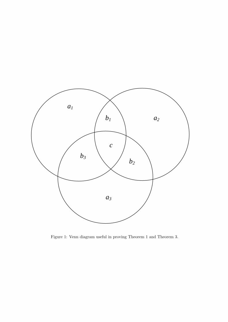
a1

a2

a3

b3

b1

b2

c

Figure 1: Venn diagram useful in proving Theorem 1 and Theorem 3.