SISSA - Universita di Trieste

Corso di Laurea Magistrale in Matematica

A. A. 2009/2010

Istituzioni di Fisica Matematica, Modulo A

Boris DUBROVIN, with additions by M. Bertola

April 10, 2019

Contents

1 Linear differential operators 3

1.1 Definitions and main examples . . . . . . . . . . . . . . . . . . . . . . . . . . . . . . 3

1.2 Principal symbol of a linear differential operator . . . . . . . . . . . . . . . . . . . . 4

1.3 Change of independent variables . . . . . . . . . . . . . . . . . . . . . . . . . . . . . 6

1.4 Canonical form of linear differential operators of order ≤ 2 with constant coefficients 7

1.5 Elliptic and hyperbolic operators. Characteristics . . . . . . . . . . . . . . . . . . . . 8

1.6 Reduction to a canonical form of second order linear differential operators in a two-dimensional space . . . . . . . . . . . . . . . . . . . . . . . . . . . . . . . . . . . . . . 11

1.7 General solution of a second order hyperbolic equation with constant coefficients inthe two-dimensional space . . . . . . . . . . . . . . . . . . . . . . . . . . . . . . . . . 14

1.8 Exercises to Section 1 . . . . . . . . . . . . . . . . . . . . . . . . . . . . . . . . . . . 15

2 Wave equation 16

2.1 Vibrating string . . . . . . . . . . . . . . . . . . . . . . . . . . . . . . . . . . . . . . . 16

2.2 D’Alembert formula . . . . . . . . . . . . . . . . . . . . . . . . . . . . . . . . . . . . 18

2.3 Some consequences of the D’Alembert formula . . . . . . . . . . . . . . . . . . . . . 20

2.4 Semi-infinite vibrating string . . . . . . . . . . . . . . . . . . . . . . . . . . . . . . . 21

2.5 Periodic problem for wave equation. Introduction to Fourier series . . . . . . . . . . 24

2.6 Finite vibrating string. Standing waves . . . . . . . . . . . . . . . . . . . . . . . . . . 32

2.7 Energy of vibrating string . . . . . . . . . . . . . . . . . . . . . . . . . . . . . . . . . 34

2.8 Inhomogeneous wave equation: Duhamel principle . . . . . . . . . . . . . . . . . . . 37

2.9 The weak solutions of the wave equation . . . . . . . . . . . . . . . . . . . . . . . . . 39

2.10 Exercises to Section 2 . . . . . . . . . . . . . . . . . . . . . . . . . . . . . . . . . . . 41

3 Laplace equation 44

3.1 Ill-posedness of the Cauchy problem for the Laplace equation . . . . . . . . . . . . . 44

3.2 Dirichlet and Neumann problems for Laplace equation on the plane . . . . . . . . . . 46

3.3 Properties of harmonic functions: mean value theorem, the maximum principle . . . 55

1

3.3.1 Boundary problem on annuli . . . . . . . . . . . . . . . . . . . . . . . . . . . 59

3.3.2 Laplace equation on rectangles . . . . . . . . . . . . . . . . . . . . . . . . . . 59

3.3.3 Poisson equation . . . . . . . . . . . . . . . . . . . . . . . . . . . . . . . . . . 61

3.4 Harmonic functions on the plane and complex analysis . . . . . . . . . . . . . . . . . 65

3.4.1 Conformal maps in fluid-dynamics . . . . . . . . . . . . . . . . . . . . . . . . 72

3.5 Exercises to Section 4 . . . . . . . . . . . . . . . . . . . . . . . . . . . . . . . . . . . 72

4 Heat equation 74

4.1 Derivation of the heat equation . . . . . . . . . . . . . . . . . . . . . . . . . . . . . . 74

4.2 Main boundary value problems for heat equation . . . . . . . . . . . . . . . . . . . . 75

4.3 Fourier transform . . . . . . . . . . . . . . . . . . . . . . . . . . . . . . . . . . . . . . 76

4.4 Solution to the Cauchy problem for heat equation on the line . . . . . . . . . . . . . 80

4.5 Mixed boundary value problems for the heat equation . . . . . . . . . . . . . . . . . 82

4.6 More general boundary conditions for the heat equation. Solution to the inhomoge-neous heat equation . . . . . . . . . . . . . . . . . . . . . . . . . . . . . . . . . . . . 86

4.7 Exercises to Section 5 . . . . . . . . . . . . . . . . . . . . . . . . . . . . . . . . . . . 89

5 Introduction to nonlinear PDEs 90

5.1 Method of characteristics for the first order quasilinear equations . . . . . . . . . . . 90

5.2 Higher order perturbations of the first order quasilinear equations. Solution of theBurgers equation . . . . . . . . . . . . . . . . . . . . . . . . . . . . . . . . . . . . . . 96

5.3 Asymptotics of Laplace integrals. Stationary phase asymptotic formula . . . . . . . 101

5.4 Dispersive waves. Solitons for KdV . . . . . . . . . . . . . . . . . . . . . . . . . . . . 105

5.5 Exercises to Section 6 . . . . . . . . . . . . . . . . . . . . . . . . . . . . . . . . . . . 108

6 Cauchy problem for systems of PDEs. Cauchy - Kovalevskaya theorem 110

6.1 Formulation of Cauchy problem . . . . . . . . . . . . . . . . . . . . . . . . . . . . . . 110

6.2 Cauchy - Kovalevskaya theorem . . . . . . . . . . . . . . . . . . . . . . . . . . . . . . 111

2

Chapter 1

Linear differential operators

1.1 Definitions and main examples

Let Ω ⊂ Rd be an open subset. Denote C∞(Ω) the set of all infinitely differentiable complex valuedsmooth functions on Ω. The Euclidean coordinates on Rd will be denoted x1, . . . , xd. We will useshort notations for the derivatives

∂k =∂

∂xk

and we also introduce operators

Dk = −i ∂k, k = 1, . . . , d. (1.1.1)

For a multiindexp = (p1, . . . , pd)

denote

|p| = p1 + · · ·+ pd

p! = p1! . . . pd!

xp = xp11 . . . xpdd∂p = ∂p11 . . . ∂pdd , Dp = Dp1

1 . . . Dpdd .

The derivatives, as well as the higher order operators Dp define linear operators

Dp : C∞(Ω)→ C∞(Ω), f 7→ Dpf = (−i)|p| ∂|p|f

∂xp11 . . . ∂xpdd.

More generally, we will consider linear differential operators of the form

A =∑|p|≤m

ap(x)Dp

ap(x) ∈ C∞(Ω) (1.1.2)

A : C∞(Ω)→ C∞(Ω).

We will define the order of the linear differential operator by

ordA = max|p| such that ap(x) 6= 0. (1.1.3)

3

Main examples are

1. Laplace operator∆ = ∂2

1 + · · ·+ ∂2d = −(D2

1 + . . . D2d) (1.1.4)

2. Heat operator∂

∂t−∆ (1.1.5)

acting on functions on the (d+ 1)-dimensional space with the coordinates (t, x1, . . . , xd).

3. Wave operator∂2

∂t2−∆. (1.1.6)

4. Schrodinger operator

i∂

∂t+ ∆. (1.1.7)

1.2 Principal symbol of a linear differential operator

Symbol of a linear differential operator (1.1.2) is a function

a(x, ξ) =∑|p|≤m

ap(x)ξp, x ∈ Ω ⊂ Rd, ξ ∈ Rd. (1.2.1)

If the order of the operator is equal to m then the principal symbol is defined by

am(x, ξ) =∑|p|=m

ap(x)ξp. (1.2.2)

The symbols (1.2.1), (1.2.2) are polynomials in d variables ξ1, . . . , ξd with coefficients being smoothfunctions on Ω.

For the above examples we have the following symbols

1. For the Laplace operator ∆ the symbol and principal symbol coincide

a = a2 = −(ξ21 + · · ·+ ξ2

d) ≡ −ξ2.

2. For the heat equation the full symbol is

a = i τ + ξ2

while the principal symbol is ξ2.

3. For the wave operator again the symbol and principal symbols coincide

a = a2 = −τ2 + ξ2.

4. The symbol of the Schrodinger operator is

−(τ + ξ2)

while the principal symbol is ξ2.

4

Exercise 1.1 Prove the following formula for the symbol of a linear differential operator

a(x, iξ) = e−i x·ξA(ei x·ξ

). (1.2.3)

Here we use the notationx · ξ = x1ξ1 + · · ·+ xd · ξd

for the natural pairing Rd × Rd → R.

Exercise 1.2 Given a linear differential operator A with constant coefficients denote a(ξ) its sym-bol (it does not depend on x for linear differential operators with constant coefficients). Prove thatthe exponential function

u(x) = ei x·ξ

is a solution to the linear differential equation

Au = 0

iff the vector ξ satisfiesa(ξ) = 0.

Exercise 1.3 Prove that for a pair of smooth functions u(x), S(x) and a linear differential operatorA of order m the expression of the form

e−i λ S(x)A(u(x)ei λ S(x)

)is a polynomial in λ of degree m. Derive the following expression for the leading coefficient of thispolynomial

e−i λ S(x)A(u(x)ei λ S(x)

)= imu(x)am(x, Sx(x))λm +O(λm−1). (1.2.4)

Here

Sx =

(∂S

∂x1, . . . ,

∂S

∂xd

)is the gradient of the function S(x).

Exercise 1.4 Let A and B be two linear differential operators of orders k and l with the principalsymbols ak(x, ξ) and bl(x, ξ) respectively. Prove that the superposition C = A B is a lineardifferential operator of order ≤ k + l. Prove that the principal symbol of C is equal to

ck+l(x, ξ) = ak(x, ξ) bl(x, ξ) (1.2.5)

in the case ordC = ordA+ ordB. In the case of strict inequality ordC < ordA+ ordB prove thatthe product (1.2.5) of principal symbols is identically equal to zero.

The formula for computing the full symbol of the product of two linear differential operators ismore complicated. We will give here the formula for the particular case of one spatial variable x.

Exercise 1.5 Let a(x, ξ) and b(x, ξ) be the symbols of two linear differential operators A and Bwith one spatial variable. Prove that the symbol of the superposition A B is equal to

a ? b =∑k≥0

(−i)k

k!∂kξ a ∂

kxb. (1.2.6)

5

1.3 Change of independent variables

Let us now analyze the transformation rules of the principal symbol a(x, ξ) of an operator A undersmooth invertible changes of variables

yi = yi(x), i = 1, . . . , n. (1.3.1)

Recall that the first derivatives transform according to the chain rule

∂

∂xi=

d∑k=1

∂yk∂xi

∂

∂yk. (1.3.2)

The transformation law of higher order derivatives is more complicated. For example

∂2

∂xi∂xj=

d∑k,l=1

∂yk∂xi

∂yl∂xj

∂2

∂yk∂yl+

d∑k=1

∂2yk∂xi∂xj

∂

∂yk

etc. However it is clear that after the transformation one obtains again a linear differential operatorof the same order m. More precisely define the operator

A =∑

(−i)|p|ap(y)∂|p|

∂yp11 . . . ∂ypdd

by the equation

Af(y(x)) =(A f(y)

)y=y(x)

.

The transformation law of the principal symbol is of particular simplicity as it follows from thefollowing

Proposition 1.6 Let am(x, ξ) be the principal symbol of a linear differential operator A. Denoteam(y, ξ) the principal symbol of the same operator written in the coordinates y, i.e., the principalsymbol of the operator A. Then

am(y(x), ξ) = am(x, ξ) provided ξi =

d∑k=1

∂yk∂xi

ξk. (1.3.3)

Proof: Applying the formula (1.2.4) one easily derives the equality

am(x, Sx) = am(y, Sy)

y = y(x)

Sx =

(∂S

∂x1, . . . ,

∂S

∂xd

), Sy =

(∂S

∂y1, . . . ,

∂S

∂yd

).

Applying the chain rule

∂S

∂xi=

d∑k=1

∂yk∂xi

∂S

∂yk

6

we arrive at the transformation rule (1.3.3) for the particular case

ξi =∂S

∂xi, ξk =

∂S

∂yk.

This proves the proposition since the gradients can take arbitrary values.

1.4 Canonical form of linear differential operators of order ≤ 2with constant coefficients

Consider a first order linear differential operator

A = a1∂

∂x1+ · · ·+ ad

∂

∂xd(1.4.1)

with constant coefficients a1, . . . , ad. One can find a linear transformation of the coordinates

ξi =d∑

k=1

ckiξk, i = 1, . . . , d (1.4.2)

that maps the vector a = (a1, . . . , ad) to the unit coordinate vector of the axis yd. After such atransformation the operator A becomes the partial derivative operator

A =∂

∂yd.

Therefore the general solution of the first order linear differential equation

Aϕ = 0

can be written in the formϕ(y1, . . . , yd) = ϕ0(y1, . . . , yd−1). (1.4.3)

Here ϕ0 is an arbitrary smooth function of (d− 1) variables.

Exercise 1.7 Prove that the general solution to the equation

Aϕ+ b ϕ = 0 (1.4.4)

with A of the form (1.4.1) and a constant b reads

ϕ(y1, . . . , yd) = ϕ0(y1, . . . , yd−1)e−b yd

for an arbitrary C1 function ϕ0(y1, . . . , yd−1).

Consider now a second order linear differential operator of the form

A =

d∑i,j=1

aij∂2

∂xi∂xj+

d∑i=1

bi∂

∂xi+ c (1.4.5)

7

with constant coefficients. Without loss of generality one can assume the coefficient matrix aij tobe symmetric. Denote

Q(ξ) = −a2(x, ξ) =

d∑i,j=1

aijξiξj (1.4.6)

the quadratic form coinciding with the principal symbol, up to a common sign. Recall the followingtheorem from linear algebra.

Theorem 1.8 There exists a linear invertible change of variables of the form (1.4.2) reducing thequadratic form (1.4.6) to the form

Q = ξ21 + · · ·+ ξ2

p − ξ2p+1 − · · · − ξ2

p+q. (1.4.7)

The numbers p ≥ 0, q ≥ 0, p+ q ≤ d do not depend on the choice of the reducing transformation.

Note that, according to the Proposition 1.6 the transformation (1.4.2) corresponds to the linearinvertible change of independent variables x→ y of the form

yk =

d∑i=1

ckixi, k = 1, . . . , d. (1.4.8)

Invertibility means that the coefficient matrix of the transformation does not degenerate:

det (cki)1≤k,i≤d 6= 0.

We arrive at

Corollary 1.9 A second order linear differential operator with constant coefficients can be reducedto the form

A =∂2

∂y21

+ · · ·+ ∂2

∂y2p

− ∂2

∂y2p+1

− · · · − ∂2

∂y2p+q

+

d∑k=1

bkyk + c (1.4.9)

by a linear transformation of the form (1.4.8). The numbers p and q do not depend on the choiceof the reducing transformation.

1.5 Elliptic and hyperbolic operators. Characteristics

Let am(x, ξ) be the principal symbol of a linear differential operator A.

Definition 1.10 It is said that the operator A : C∞(Ω)→ C∞(Ω) is elliptic if

am(x, ξ) 6= 0 for any ξ 6= 0, x ∈ Ω. (1.5.1)

8

For example the Laplace operator

∆ =∂2

∂x21

+ · · ·+ ∂2

∂x2n

is elliptic on Ω = Rd. The Tricomi operator

A =∂2

∂x2+ x

∂2

∂y2(1.5.2)

is elliptic on the right half plane x > 0.

Definition 1.11 Given a point x0 ∈ Ω, the hypersurface in the ξ-space defined by the equation

am(x0, ξ) = 0 (1.5.3)

is called characteristic cone of the operator A at x0. The vectors ξ satisfying (1.5.3) are calledcharacteristic vectors at the point x0.

Observe that the hypersurface (1.5.3) is invariant with respect to rescalings

ξ 7→ λξ ∀ λ ∈ R (1.5.4)

since the polynomial am(x0, ξ) is homogeneous of degree m:

am(x, λ ξ) = λmam(x, ξ).

The characteristic cone of an elliptic operator is one point ξ = 0. For the example of waveoperator

A =∂2

∂t2−∆, ∆ =

∂2

∂x21

+ · · ·+ ∂2

∂x2d

(1.5.5)

the characteristic cone is given by the equation

τ2 − ξ21 − · · · − ξ2

d = 0. (1.5.6)

Thus it coincides with the standard cone in the Euclidean (d+ 1)-dimensional space. The charac-teristic cone of the heat operator

∂

∂t−∆ (1.5.7)

is the τ -lineξ1 = · · · = ξd = 0. (1.5.8)

Definition 1.12 The hypersurface in Rd is called characteristic surface or simply characteristicsfor the operator A if at every point x of the surface the normal vector ξ is a characteristic vector:

am(x, ξ) = 0.

If the hypesurface is defined by a local equation

S(x) = 0 (1.5.9)

then S(x) satisfies the equationam (x, Sx(x)) = 0 (1.5.10)

at every point of the hypersurface (1.5.9).

9

As it follows from the Proposition 1.6 the characteristics do not depend on the choice of asystem of coordinates.

Example. For a first order linear differential operator

A = a1(x)∂

∂x1+ · · ·+ ad(x)

∂

∂xd(1.5.11)

the function S(x) defining a characteristic hypersurface must satisfy the equation

AS(x) = 0. (1.5.12)

It is therefore a first integral of the following system of ODEs

x1 = a1(x1, . . . , xd)

. . . (1.5.13)

xd = ad(x1, . . . , xd)

Indeed, the equation (1.5.12) says that the function S(x) is constant along the integral curves ofthe system (1.5.13). It is known from the theory of ordinary differential equations that locally, neara point x0 such that

(a1(x0), . . . , ad(x

0))6= 0 there exists a smooth invertible change of coordinates

(x1, . . . , xd) 7→ (y1, . . . , yd), yk = yk(x1, . . . , xd)

such that, in the new coordinates the system reduces to the form

y1 = 0

. . . (1.5.14)

yd−1 = 0

yd = 1

(the so-called rectification of a vector field). For the particular case of constant coefficients theneeded transformation is linear (see above). In these coordinates the general solution to the equation(1.5.12) reads

S(y1, . . . , yd) = S0(y1, . . . , yd−1). (1.5.15)

Hyperbolic operators. Let us consider a linear differential operator A acting on smooth func-tions on a domain Ω in the (d + 1)-dimensional space with Euclidean coordinates (t, x1, . . . , xd).Denote am(t, x, τ, ξ) the principal symbol of this operator. Here

τ ∈ R, ξ = (ξ1, . . . , ξd) ∈ Rd.

Recall that the principal symbol of an operator of order m is a polynomial of degree m in τ , ξ1,. . . , ξd.

Definition 1.13 The linear differential operator A is called hyperbolic with respect to the timevariable t if for any fixed ξ 6= 0 and any (t, x) ∈ Ω the equation for τ

am(t, x, τ, ξ) = 0 (1.5.16)

has m pairwise distinct real roots

τ1(t, x, ξ), . . . , τm(t, x, ξ).

10

For brevity we will often say that a linear differential operator is hyperbolic if all its character-istics are real and pairwise distinct. For elliptic operators the characteristics are purely imaginary.

The wave operator (1.5.5) gives a simple example of a hyperbolic operator. Indeed, the equation

τ2 = ξ21 + · · ·+ ξ2

d

has two distinct roots

τ = ±√ξ2

1 + · · ·+ ξ2d

for any ξ 6= 0. The heat operator (1.5.7) is neither hyperbolic nor elliptic.

Finding the j-th characteristic of a hyperbolic operator requires knowledge of solutions to thefollowing Hamilton–Jacobi equation for the functions S = S(x, t)

∂S

∂t= τj

(t, x,

∂S

∂x

). (1.5.17)

From the course of analytical mechanics it is known that the latter problem is reduced to integratingthe Hamilton equations

xi = ∂H(t,x,p)∂pi

pi = −∂H(t,x,p)∂xi

(1.5.18)

with the time-dependent Hamiltonian H(t, x, p) = τj(t, x, p). In the next section we will considerthe particular case d = 1 and apply it to the problem of canonical forms of the second order lineardifferential operators in a two-dimensional space.

1.6 Reduction to a canonical form of second order linear differen-tial operators in a two-dimensional space

Consider a linear differential operator

A = a(x, y)∂2

∂x2+ 2b(x, y)

∂2

∂x∂y+ c(x, y)

∂2

∂y2, (x, y) ∈ Ω ⊂ R2. (1.6.1)

The characteristics of these operator are curves

x = x(t), y = y(t).

Here t is some parameter on the characteristic. Let (dx, dy) be the tangent vector to the curve.Then the normal vector (−dy, dx) must satisfy the equation

a(x, y)dy2 − 2b(x, y)dx dy + c(x, y)dx2 = 0. (1.6.2)

Assuming a(x, y) 6= 0 one obtains a quadratic equation for the vector dy/dx

a(x, y)

(dy

dx

)2

− 2b(x, y)dy

dx+ c(x, y) = 0. (1.6.3)

The operator (1.6.1) is hyperbolic iff the discriminant of this equation is positive:

b2 − a c > 0. (1.6.4)

11

For elliptic operators the discriminant is strictly negative.

For a hyperbolic operator one has two families of characteristics to be found from the ODEs

dy

dx=b(x, y) +

√b2(x, y)− a(x, y) c(x, y)

a(x, y)(1.6.5)

dy

dx=b(x, y)−

√b2(x, y)− a(x, y) c(x, y)

a(x, y). (1.6.6)

Letφ(x, y) = c1, ψ(x, y) = c2 (1.6.7)

be the equations of the characteristics1. Here c1 and c2 are two integration constants. Such curvespass through any point (x, y) ∈ Ω. Moreover they are not tangent at every point. Let us introducenew local coordinates u, v by

u = φ(x, y), v = ψ(x, y). (1.6.8)

Lemma 1.14 The change of coordinates

(x, y) 7→ (u, v)

is locally invertible. Moreover the inverse functions

x = x(u, v), y = y(u, v)

are smooth.

Proof: We have to check non-vanishing of the Jacobian

det

(∂u/∂x ∂u/∂y∂v/∂x ∂v/∂y

)= det

(φx φyψx ψy

)6= 0. (1.6.9)

By definition the first derivatives of the functions φ and ψ correspond to two different roots of thesame quadratic equation

a(x, y)φ2x + 2b(x, y)φxφy + c(x, y)φ2

y = 0, a(x, y)ψ2x + 2b(x, y)ψxψy + c(x, y)ψ2

y = 0.

The determinant (1.6.9) vanishes iff the gradients of φ and ψ are proportional:

(φx, φy) ∼ (ψx, ψy).

This contradicts the requirement to have the roots distinct.

Let us rewrite the linear differential operator A in the new coordinates:

A = a(u, v)∂2

∂u2+ 2b(u, v)

∂2

∂u∂v+ c(u, v)

∂2

∂v2+ . . . (1.6.10)

where the dots stand for the terms with the low order derivatives.

1The function φ(x, y), resp. ψ(x, y), is a first integral for the ODE (1.6.5), resp. (1.6.6), that is, it takes constantvalues along the integral curves of this differential equation.

12

Theorem 1.15 In the new coordinates the linear differential operator reads

A = 2b(u, v)∂2

∂u ∂v+ . . .

Proof: In the new coordinates the characteristic have the form

u = c1, v = c2

for arbitrary constants c1 and c2. Therefore their tangent vectors (1, 0) and (0, 1) must satisfy theequation for characteristics

a(u, v)dv2 − 2b(u, v)du dv + c(u, v)dv2 = 0.

This implies a(u, v) = c(u, v) = 0.

For the case of elliptic operator (1.6.1) the analogue of the differential equations (1.6.5), (1.6.6)are complex conjugated equations

dy

dx=b± i

√a c− b2a

, a = a(x, y), b = b(x, y), c = c(x, y). (1.6.11)

Assuming analyticity of the functions a(x, y), b(x, y), c(x, y) one can prove existence of a complexvalued first integral

S(x, y) = φ(x, y) + i ψ(x, y) (1.6.12)

satisfying

aSx +(b− i

√a c− b2

)Sy = 0. (1.6.13)

Let us introduce new system of coordinates by

u = φ(x, y), v = ψ(x, y). (1.6.14)

Exercise 1.16 Prove that the transformation

(x, y) 7→ (u, v)

is locally smoothly invertible. Prove that the operator A in the new coordinates takes the form

A = a(u, v)

(∂2

∂u2+

∂2

∂v2

)+ . . . (1.6.15)

with some nonzero smooth function a(u, v). Like above the dots stand for the terms with lowerorder derivatives.

13

Let us now consider the case of linear differential operators of the form (1.6.1) with identicallyvanishing discriminant

b2(x, y)− a(x, y) c(x, y) ≡ 0. (1.6.16)

Operators of this class are called parabolic. In this case we have only one characteristic to be foundfrom the equation

dy

dx=b(x, y)

a(x, y). (1.6.17)

Let φ(x, y) be a first integral of this equation

aφx + b φy = 0, φ2x + φ2

y 6= 0. (1.6.18)

Choose an arbitrary smooth function ψ(x, y) such that

det

(φx φyψx ψy

)6= 0.

In the coordinatesu = φ(x, y), v = ψ(x, y)

the coefficient a(u, v) vanishes, since the line φ(x, y) = const is a characteristic. But then thecoefficient b(u, v) must vanish either because of vanishing of the discriminant

b2 − a c = 0.

Thus the canonical form of a parabolic operator is

A = c(u, v)∂2

∂v2+ . . . (1.6.19)

where the dots stand for the terms of lower order.

1.7 General solution of a second order hyperbolic equation withconstant coefficients in the two-dimensional space

Consider a hyperbolic operator

A = a∂2

∂x2+ 2b

∂2

∂x ∂y+ c

∂2

∂y2(1.7.1)

with constant coefficients a, b, c satisfying the hyperbolicity condition

b2 − a c > 0.

The equations for characteristics (1.6.5), (1.6.6) can be easily integrated. This gives two linear firstintegrals

u = y − λ1x, v = y − λ2x

(1.7.2)

λ1,2 =b±√b2 − a ca

.

14

In the new coordinates the hyperbolic equation Aϕ = 0 reduces to

∂2ϕ

∂u∂v= 0. (1.7.3)

The general solution to this equation can be written in the form

ϕ = f(y − λ1x) + g(y − λ2x) (1.7.4)

where f and g are two arbitrary smooth2 functions of one variable.

For example consider the wave equation

ϕtt = a2ϕxx (1.7.5)

where a is a positive constant. The general solution reads

ϕ(x, t) = f(x− a t) + g(x+ a t). (1.7.6)

Observe that f(x − a t) is a right-moving wave propagating with constant speed a. In a similarway g(x+ a t) is a left-moving wave. Therefore the general solution to the wave equation (1.7.5) isa superposition of two such waves.

1.8 Exercises to Section 1

Exercise 1.17 Reduce to the canonical form the following equations

uxx + 2uxy − 2uxz + 2uyy + 6uzz = 0 (1.8.1)

uxy − uxz + ux + uy − uz = 0. (1.8.2)

Exercise 1.18 Reduce to the canonical form the following equations

x2uxx + 2x y uxy − 3y2uyy − 2xux + 4y uy + 16x4u = 0 (1.8.3)

y2uxx + 2x y uxy + 2x2uyy + y uy = 0 (1.8.4)

uxx − 2uxy + uyy + ux + uy = 0 (1.8.5)

Exercise 1.19 Find general solution to the following equations

x2uxx − y2uyy − 2y uy = 0 (1.8.6)

x2uxx − 2x y uxy + y2uyy + xux + y uy = 0. (1.8.7)

2It suffices to take the functions of the C2 class.

15

Chapter 2

Wave equation

2.1 Vibrating string

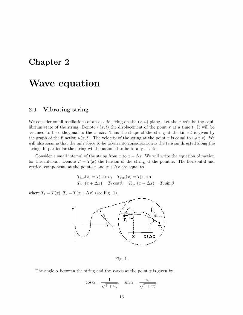
We consider small oscillations of an elastic string on the (x, u)-plane. Let the x-axis be the equi-librium state of the string. Denote u(x, t) the displacement of the point x at a time t. It will beassumed to be orthogonal to the x-axis. Thus the shape of the string at the time t is given bythe graph of the function u(x, t). The velocity of the string at the point x is equal to ut(x, t). Wewill also assume that the only force to be taken into consideration is the tension directed along thestring. In particular the string will be assumed to be totally elastic.

Consider a small interval of the string from x to x+ ∆x. We will write the equation of motionfor this interval. Denote T = T (x) the tension of the string at the point x. The horizontal andvertical components at the points x and x+ ∆x are equal to

Thor(x) = T1 cosα, Tvert(x) = T1 sinα

Thor(x+ ∆x) = T2 cosβ, Tvert(x+ ∆x) = T2 sinβ

where T1 = T (x), T2 = T (x+ ∆x) (see Fig. 1).

Fig. 1.

The angle α between the string and the x-axis at the point x is given by

cosα =1√

1 + u2x

, sinα =ux√

1 + u2x

.

16

The oscillations are assumed to be small. More precisely this means that the term ux is small. Soat the leading approximation we can neglect the square of it to arrive at

cosα ' 1, sinα ' ux(x)

cosβ ' 1, sinβ ' ux(x+ ∆x)

So the horizontal and vertical components at the points x and x+ ∆x are equal to

Thor(x) ' T1, Tvert(x) ' T1ux(x)

Thor(x+ ∆x) ' T2, Tvert(x+ ∆x) = T2ux(x+ ∆(x),

Since the string moves in the u-direction, the horizontal components at the points x and x + ∆xmust coincide:

T1 = T (x) = T (x+ ∆x) = T2.

Therefore T (x) ≡ T = const.

Let us now consider the vertical components. The resulting force acting on the piece of thestring is equal to

f = T2 sinβ − T1 sinα = T ux(x+ ∆x)− T ux(x) ' T uxx(x) ∆x.

On another side the vertical component of the total momentum of the piece of the string is equalto

p =

∫ x+∆x

xρ(x)ut(x, t) ds(x) ' ρ(x)ut(x, t) ∆x

where ρ(x) is the linear mass density of the string and

ds(x) =dx√

1 + u2x(x)

' dx

is the element of the length1. The second Newton law

pt = f

in the limit ∆x→ 0 yieldsρ(x)utt = T uxx.

In particular in the case of constant mass density one arrives at the equation

utt = a2uxx (2.1.1)

where the constant a is defined by

a2 =T

ρ. (2.1.2)

1This means that the length s of the segment of the string between x = x1 and x = x2 is equal to

s =

∫ x2

x1

ds(x),

and the total mass m of the same segment is equal to

m =

∫ x2

x1

ρ(x) ds(x).

17

Exercise 2.1 Prove that the plane wave

u(x, t) = Aei(k x+ω t) (2.1.3)

satisfies the wave equation (2.1.1) if and only if the real parameters ω and k satisfy the followingdispersion relation

ω = ±a k. (2.1.4)

The parameters ω and k are called resp. the frequency2 and wave number of the plane wave.The arbitrary parameter A is called the amplitude of the wave. It is clear that the plane wave isperiodic in x with the period

L =2π

k(2.1.5)

since the exponential function is periodic with the period 2π i. The plane wave is also periodic int with the period

T =2π

ω. (2.1.6)

Due to linearity of the wave equation the real and imaginary parts of the solution (2.1.3) solve thesame equation (2.1.1). Assuming A to be real we thus obtain the real valued solutions

Reu = A cos(k x+ ω t), Imu = A sin(k x+ ω t). (2.1.7)

2.2 D’Alembert formula

Let us start with considering oscillations of an infinite string. That is, the spatial variable x variesfrom −∞ to ∞. The Cauchy problem for the equation (2.1.1) is formulated in the following way:find a solution u(x, t) defined for t ≥ 0 such that at t = 0 the initial conditions

u(x, 0) = φ(x), ut(x, 0) = ψ(x) (2.2.1)

hold true. The solution is given by the following D’Alembert formula:

Theorem 2.2 (D’Alembert formula) For arbitrary initial data φ(x) ∈ C2(R), ψ(x) ∈ C1(R)the solution to the Cauchy problem (2.1.1), (2.2.1) exists and is unique. Moreover it is given by theformula

u(x, t) =φ(x− a t) + φ(x+ a t)

2+

1

2a

∫ x+a t

x−a tψ(s) ds. (2.2.2)

Proof: As we have proved in Section 1.7 the general solution to the equation (2.1.1) can berepresented in the form

u(x, t) = f(x− a t) + g(x+ a t). (2.2.3)

2In physics literature the number −ω is called frequency.

18

Let us choose the functions f and g in order to meet the initial conditions (2.2.1). We obtain thefollowing system:

f(x) + g(x) = φ(x)

(2.2.4)

a[g′(x)− f ′(x)

]= ψ(x).

Integrating the second equation yields

g(x)− f(x) =1

a

∫ x

x0

ψ(s) ds+ C

where C is an integration constant. So

f(x) =1

2φ(x)− 1

2a

∫ x

x0

ψ(s) ds− 1

2C

g(x) =1

2φ(x) +

1

2a

∫ x

x0

ψ(s) ds+1

2C.

Thus

u(x, t) =1

2φ(x− a t)− 1

2a

∫ x−a t

x0

ψ(s) ds+1

2φ(x+ a t) +

1

2a

∫ x+a t

x0

ψ(s) ds.

This gives (2.2.2). It remains to check that, given a pair of functions φ(x) ∈ C2, ψ(x) ∈ C1 theD’Alembert formula yields a solution to (2.1.1). Indeed, the function (2.2.2) is twice differentiablein x and t. It remains to substitute this function into the wave equation and check that the equationis satisfied. We leave it as an exercise for the reader. It is also straightforward to verify validity ofthe initial data (2.2.1).

Example. For the constant initial data

u(x, 0) = u0, ut(x, 0) = v0

the solution has the formu(x, t) = u0 + v0t.

This solution corresponds to the free motion of the string with the constant speed v0.

Moreover the solution to the wave equation is stable with respect to small variations of theinitial data. Namely,

Exercise 2.3 For any ε > 0 and any T > 0 there exists δ > 0 such that the solutions u(x, t) andu(x, t) of the two Cauchy problems with initial conditions (2.2.1) and

u(x, 0) = φ(x), ut(x, 0) = ψ(x) (2.2.5)

satisfysup

x∈R, t∈[0,T ]|u(x, t)− u(x, t)| < ε (2.2.6)

provided the initial conditions satisfy

supx∈R|φ(x)− φ(x)| < δ, sup

x∈R|ψ(x)− ψ(x)| < δ. (2.2.7)

Remark 2.4 The property formulated in the above exercise is usually referred to as well posednessof the Cauchy problem (2.1.1), (2.2.1). We will return later to the discussion of this importantproperty.

19

2.3 Some consequences of the D’Alembert formula

Let (x0, t0) be a point of the (x, t)-plane, t0 > 0. As it follows from the D’Alembert formula thevalue of the solution at the point (x0, t0) depends only on the values of φ(x) at x = x0 ± a t0and value of ψ(x) on the interval [x0 − a t0, x0 + a t0]. The triangle with the vertices (x0, t0) and(x0 ± a t0, 0) is called the dependence domain of the segment [x0 − a t0, x0 + a t0]. The values ofthe solution inside this triangle are completely determined by the values of the initial data on thesegment.

Fig. 2. The dependence domain of the segment [x0 − a t0, x0 + a t0].

Another important definition is the influence domain for a given segment [x1, x2] consider thedomain defined by inequalities

x+ a t ≥ x1, x− a t ≤ x2, t ≥ 0. (2.3.1)

Changing the initial data on the segment [x1, x2] will not change the solution u(x, t) outside theinfluence domain.

Fig. 3. The influence domain of the segment [x1, x2].

Remark 2.5 It will be convenient to slightly extend the class of initial data admitting piecewisesmooth functions φ(x), ψ(x) (all singularities of the latter must be integrable). If xj are the singu-larities of these functions, j = 1, 2, . . . , then the solution u(x, t) given by the D’Alembert formulawill satisfy the wave equation outside the lines

x = ±a t+ xj , t ≥ 0, j = 1, 2, . . .

The above formula says that the singularities of the solution propagate along the characteristics.

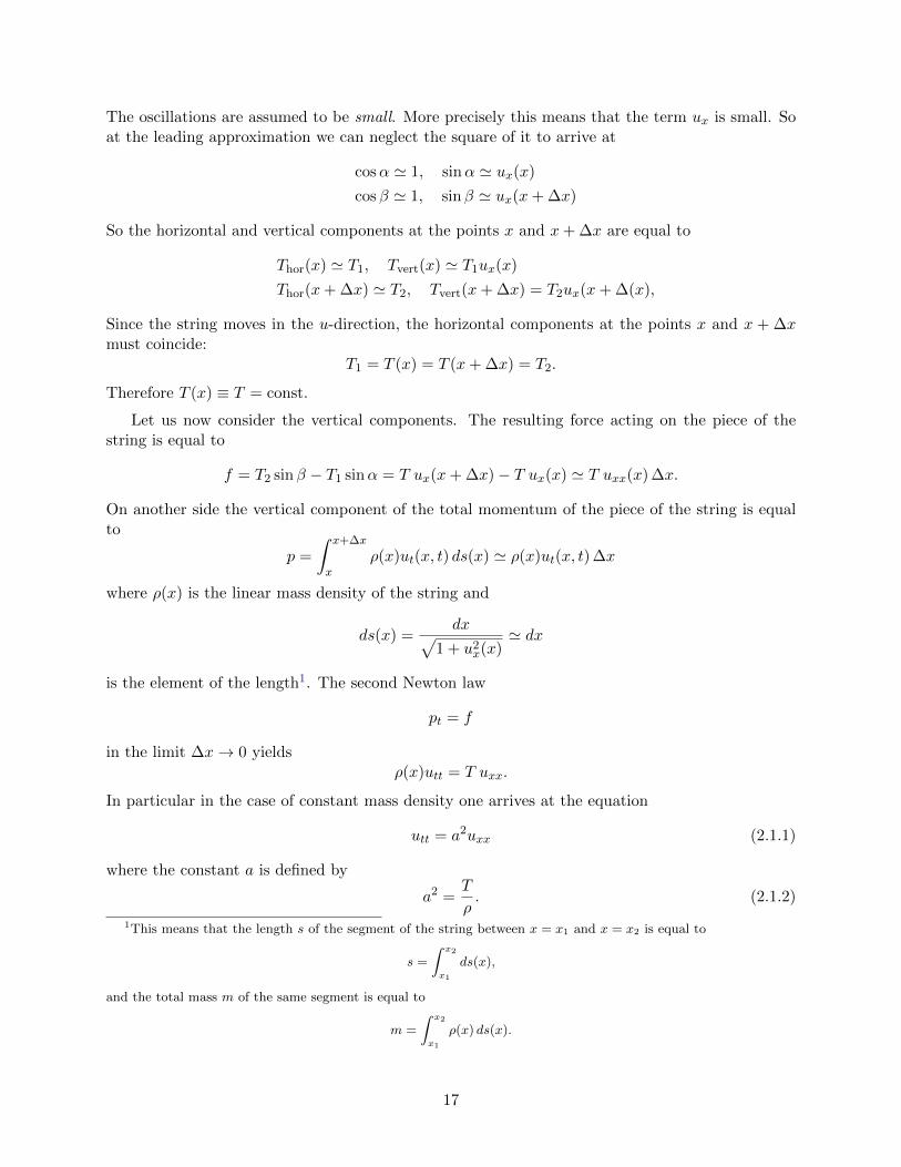
Example. Let us draw the profile of the string for the triangular initial data φ(x) shown onFig. 4 and ψ(x) ≡ 0.

20

Fig. 4. The solution of the Cauchy problem for wave equation on the real line with a triangularinitial profile at different instants of time.

2.4 Semi-infinite vibrating string

Let us begin with the following simple observation.

Lemma 2.6 Let u(x, t) be a solution to the wave equation. Then so are the functions

±u(±x,±t)

with arbitrary choices of all three signs.

Proof: This follows from linearity of the wave equation and from its invariance with respect tothe spatial reflection

x 7→ −x

and time inversiont 7→ −t.

21

Let us consider oscillations of a string with a fixed point. Without loss of generality we canassume that the fixed point is at x = 0. We arrive at the following Cauchy problem for (2.1.1) onthe half-line x > 0:

u(x, 0) = φ(x), ut(x, 0) = ψ(x), x > 0. (2.4.1)

The solution must also satisfy the boundary condition

u(0, t) = 0, t ≥ 0. (2.4.2)

The problem (2.1.1), (2.4.1), (2.4.2) is often called mixed problem since we have both initial condi-tions and boundary conditions.

The solution to the mixed problem on the half-line can be reduced to the problem on the infiniteline by means of the following trick.

Lemma 2.7 Let the initial data φ(x), ψ(x) for the Cauchy problem (2.1.1), (2.2.1) be odd functionsof x. Then the solution u(x, t) is an odd function for all t.

Proof: Denoteu(x, t) := −u(−x, t).

According to Lemma 2.6 the function u(x, t) satisfies the same equation. At t = 0 we have

u(x, 0) = −u(−x, 0) = −φ(−x) = φ(x), ut(x, 0) = −ut(−x, 0) = −ψ(−x) = ψ(x)

since φ and ψ are odd functions. Therefore u(x, t) is a solution to the same Cauchy problem (2.1.1),(2.2.1). Due to uniqueness u(x, t) = u(x, t), i.e. −u(−x, t) = u(x, t) for all x and t.

We are now ready to present a recipe for solving the mixed problem for the wave equation onthe half-line. Let us extend the initial data onto entire real line as odd functions. We arrive at thefollowing Cauchy problem for the wave equation:

u(x, 0) =

φ(x), x > 0−φ(−x), x < 0

, ut(x, 0) =

ψ(x), x > 0−ψ(−x), x < 0

(2.4.3)

According to Lemma 2.7 the solution u(x, t) to the Cauchy problem (2.1.1), (2.4.3) given by theD’Alembert formula will be an odd function for all t. Therefore

u(0, t) = −u(0, t) = 0 for all t.

Example. Consider the evolution of a triangular initial profile on the half-line. The graphof the initial function φ(x) is non-zero on the interval [l, 3l]; the initial velocity ψ(x) = 0. Theevolution is shown on Fig. 5 for few instants of time. Observe the reflected profile (the dotted line)on the negative half-line.

In a similar way one can treat the mixed problem on the half-line with a free boundary. In thiscase the vertical component T ux of the tension at the left edge must vanish at all times. Thus theboundary condition (2.4.2) has to be replaced with

ux(0, t) = 0 for all t ≥ 0. (2.4.4)

22

One can solve the mixed problem (2.1.1), (2.4.1), (2.4.4) by using even extension of the initial dataonto the negative half-line. We leave the details of the construction as an exercise for the reader.

Fig. 5. The solution of the Cauchy problem for wave equation on the half-line with a triangularinitial profile.

23

2.5 Periodic problem for wave equation. Introduction to Fourierseries

Let us look for solutions to the wave equation (2.1.1) periodic in x with a given period L > 0. Thuswe are looking for a solution u(x, t) satisfying

u(x+ L, t) = u(x, t) for any t ≥ 0. (2.5.1)

The initial data of the Cauchy problem

u(x, 0) = φ(x), ut(x, 0) = ψ(x) (2.5.2)

must also be L-periodic functions.

Theorem 2.8 Given L-periodic initial data φ(x) ∈ C2(R), ψ(x) ∈ C1(R) the periodic Cauchyproblem (2.5.1), (2.5.2) for the wave equation (2.1.1) has a unique solution.

Proof: According to the results of Section 2.2 the solution u(x, t) to the Cauchy problem (2.1.1),(2.5.2) on −∞ < x <∞ exists and is unique and is given by the D’Alembert formula. Denote

u(x, t) := u(x+ L, t).

Since the coefficients of the wave equation do not depend on x the function u(x, t) satisfies thesame equation. The initial data for this function have the form

u(x, 0) = φ(x+ L) = φ(x), ut(x, t) = ψ(x+ L) = ψ(x)

because of periodicity of the functions φ(x) and ψ(x). So the initial data of the solutions u(x, t)and u(x, t) coincide. From the uniqueness of the solution we conclude that u(x, t) = u(x, t) for allx and t, i.e. the function u(x, t) is periodic in x with the same period L.

Exercise 2.9 Prove that the complex exponential function eikx is L-periodic iff the wave numberk has the form

k =2πn

L, n ∈ Z. (2.5.3)

In the following two exercises we will consider the particular case L = 2π. In this case thecomplex exponential

e2πinxL

obtained in the previous exercise reduces to einx.

Exercise 2.10 Prove that the solution of the periodic Cauchy problem with the Cauchy data

u(x, 0) = einx, ut(x, 0) = 0 (2.5.4)

is given by the formulau(x, t) = einx cosnat. (2.5.5)

24

Exercise 2.11 Prove that the solution of the periodic Cauchy problem with the Cauchy data

u(x, 0) = 0, ut(x, 0) = einx (2.5.6)

is given by the formula

u(x, t) =

einx sinnat

na , n 6= 0t, n = 0.

(2.5.7)

Using the theory of Fourier series we can represent any solution to the periodic problem to thewave equation as a superposition of the solutions (2.5.5), (2.5.7). Let us first recall some basics ofthe theory of Fourier series.

Let f(x) be a 2π-periodic continuously differentiable complex valued function on R. The Fourierseries of this function is defined by the formula∑

n∈Zcne

inx (2.5.8)

cn =1

2π

∫ 2π

0f(x)e−inxdx. (2.5.9)

The following theorem is a fundamental result of the theory of Fourier series.

Theorem 2.12 For any function f(x) satisfying the above conditions the Fourier series is uni-formly convergent to the function f(x).

In particular we conclude that any C1-smooth 2π-periodic function f(x) can be represented asa sum of uniformly convergent Fourier series

f(x) =∑n∈Z

cneinx, cn =

1

2π

∫ 2π

0f(x)e−inxdx. (2.5.10)

For completeness we remind the proof of this Theorem.

Let us introduce Hermitean inner product in the space of complex valued 2π-periodic continuousfunctions:

(f, g) =1

2π

∫ 2π

0f(x)g(x) dx. (2.5.11)

Here the bar stands for complex conjugation. This inner product satisfies the following properties:

(g, f) = (f, g) (2.5.12)

(λf1 + µf2, g) = λ(f1, g) + µ(f2, g)

(f, λg1 + µg2) = λ(f, g1) + µ(f, g2)for any λ, µ ∈ C (2.5.13)

(f, f) > 0 for any nonzero continuous function f(x). (2.5.14)

The real nonnegative number (f, f) will be used for defining the L2-norm of the function:

‖f‖ :=√

(f, f). (2.5.15)

25

Exercise 2.13 Prove that the L2-norm satisfies the triangle inequality:

‖f + g‖ ≤ ‖f‖+ ‖g‖. (2.5.16)

Observe that the complex exponentials einx form an orthonormal system with respect to theinner product (2.5.11): (

eimx, einx)

= δmn =

1, m = n0 m 6= n

. (2.5.17)

(check it!).

Let f(x) be a continuous function; denote cn its Fourier coefficients. The following formula

cn = (einx, f), n ∈ Z (2.5.18)

gives a simple interpretation of the Fourier coefficients as the coefficients of decomposition of thefunction f with respect to the orthonormal system made from exponentials. Moreover, the partialsum of the Fourier series

SN (x) =N∑

n=−Ncne

inx (2.5.19)

can be interpreted as the orthogonal projection of the vector f onto the (2N+1)-dimensional linearsubspace

VN = span(1, e±ix, e±2ix, . . . , e±iNx

)(2.5.20)

consisting of all trigonometric polynomials

PN (x) =N∑

n=−Npne

inx (2.5.21)

of degree N . Here p0, p±1, . . . p±N are arbitrary complex numbers.

Lemma 2.14 The following inequality holds true:

N∑n=−N

|cn|2 ≤ ‖f‖2. (2.5.22)

The statement of this lemma is called Bessel inequality.

Proof: We have

0 ≤ ‖f(x)−N∑

n=−Ncne

inx‖2 =

(f(x)−

N∑n=−N

cneinx, f(x)−

N∑n=−N

cneinx

)

= (f, f)−N∑

n=−N

[cn(f, einx

)+ cn

(einx, f

)]+

N∑m,n=−N

cmcn(eimx, einx

).

Using (2.5.18) and orthonormality (2.5.17) we recast the right hand side of the last equation in theform

(f, f)−N∑

n=−N|cn|2.

26

This proves Bessel inequality.

Geometrically the Bessel inequality says that the square length of the orthogonal projection ofa vector onto the linear subspace VN cannot be longer than the square length of the vector itself.

Corollary 2.15 For any continuous function f(x) the series of squares of absolute values ofFourier coefficients converges: ∑

n∈Z|cn|2 <∞. (2.5.23)

The following extremal property says that the N -th partial sum of the Fourier series gives thebest L2-approximation of the function f(x) among all trigonometric polynomials of degree N .

Lemma 2.16 For any trigonometric polynomial PN (x) of degree N the following inequality holdstrue

‖f(x)− SN (x)‖ ≤ ‖f(x)− PN (x)‖. (2.5.24)

Here SN (x) is the N -th partial sum (2.5.19) of the Fourier series of the function f . The equalityin (2.5.24) takes place iff the trigonometric polynomial PN (x) coincides with SN (x), i.e.,

pn =1

2π

∫ 2π

0f(x)e−inxdx, n = 0,±1,±2, . . . ,±N,

Proof: From (2.5.18) we derive that

(f(x)− SN (x), PN (x)) = 0 for any PN (x) ∈ VN .

Hence

‖f(x)− PN (x)‖2 = ‖(f − SN ) + (SN − PN‖2 =

= (f − SN , f − SN ) + (f − SN , QN ) + (QN , f − SN ) + (QN , QN )

= (f − SN , f − SN ) + (QN , QN ) ≥ (f − SN , f − SN ) = ‖f − SN‖2.

Here we denoteQN = SN (x)− PN (x) ∈ VN .

Clearly the equality takes place iff QN = 0, i.e. PN = SN .

Lemma 2.17 For any continuous 2π-periodic function the following Parseval equality holds true:∑n∈Z|cn|2 = ‖f‖2. (2.5.25)

The Parseval equality can be considered as an infinite-dimensional analogue of the Pythagorastheorem: sum of the squares of orthogonal projections of a vector on the coordinate axes is equalto the square length of the vector.

27

Proof: According to Stone – Weierstrass theorem3 any continuous 2π-periodic function can beuniformly approximated by Fourier polynomials

PN (x) =

N∑n=−N

pneinx. (2.5.26)

That means that for a given function f(x) and any ε > 0 there exists a trigonometric polynomialPN (x) of some degree N such that

supx∈[0,2π] |f(x)− PN (x)| < ε.

Then

‖f − PN‖2 =1

2π

∫ 2π

0|f(x)− PN (x)|2dx < ε2.

Therefore, due to the extremal property (see Lemma 2.16 above), we obtain the following inequality

‖f − SN‖2 < ε2.

Repeating the computation used in the proof of Bessel inequality

‖f − SN‖2 = ‖f‖2 −N∑

n=−N|cn|2 < ε2

we arrive at the proof of Lemma.

3The Stone – Weierstrass theorem is a very general result about uniform approximation of continuous functionson a compact K in a metric space. Let us recall this important theorem. Let A ⊂ C(K) be a subset of functions inthe space of continuous real- or complex-valued functions on a compact K. The following requirements must holdtrue.

1. A must be a subalgebra in C(K), i.e. for f, g ∈ A, α, β ∈ R (or α, β ∈ C) the linear combination and theproduct belong to A:

αf + β g ∈ A, f · g ∈ A.2. The functions in A must separate points in K, i.e., ∀x, y ∈ K, x 6= y there exists f ∈ A such that

f(x) 6= f(y).

3. The subalgebra is non-degenerate, i.e., ∀x ∈ K there exists f ∈ A such that f(x) 6= 0.The last condition has to be imposed in the complex situation.

4. The subalgebra A is said to be self-adjoint if for any function f ∈ A the complex conjugate function f also belongsto A.

Theorem 2.18 Given an algebra of functions A ⊂ C(K) that separates points, is non-degenerate and, for complex-valued functions, is self-adjoint then A is an everywhere dense subset in C(K).

Recall that density means that for any continuous function F ∈ C(K) and an arbitrary ε > 0 there exists f ∈ Asuch that

supx∈K |F (x)− f(x)| < ε.

In the particular case of algebra of polynomials one obtains the classical Weierstrass theorem about polynomialapproximations of continuous functions on a finite interval. For the needs of the theory of Fourier series one has toapply the Stone – Weierstrass theorem to the subalgebra of Fourier polynomials in the space of continuous 2π-periodicfunctions. We leave as an exercise to verify applicability of the Stone – Weierstrass theorem in this case.

28

The Parseval equality is also referred to as completeness of the trigonometric system of functions

1, e±ix, e±2ix, . . . .

For the case of infinite-dimensional spaces equipped with a Hermitean (or Euclidean) inner productthe property of completeness is the right analogue of the notion of an orthonormal basis of the space.

Corollary 2.19 Two continuous 2π-periodic functions f(x), g(x) with all equal Fourier coefficientsidentically coincide.

Proof: Indeed, the difference h(x) = f(x)− g(x) is continuous function with zero Fourier coeffi-cients. The Parseval equality implies ‖h‖2 = 0. So h(x) ≡ 0.

We can now prove that uniform convergence of the Fourier series of a C1-function. Denote c′nthe Fourier coefficients of the derivative f ′(x). Integrating by parts we derive the following formula:

cn =1

2π

∫ 2π

0f(x)e−inx dx = − 1

2πinf(x)e−inx

∣∣2π0 +

1

2πin

∫ 2π

0f ′(x)e−inx dx = − i

nc′n.

This implies convergence of the series ∑n∈Z|cn|.

Indeed,

|cn| =|c′n|n≤ 1

2

(|c′n|2 +

1

n2

).

The series∑|c′n|2 converges according to the Corollary 2.15; convergence of the series

∑ 1n2 is well

known. Using Weierstrass theorem we conclude that the Fourier series converges absolutely anduniformly ∑

n∈Z

∣∣cneinx∣∣ =∑n∈Z|cn| <∞.

Denote g(x) the sum of this series. It is a continuos function. The Fourier coefficients of g coincidewith those of f : (

einx, g)

= cn.

Hence f(x) ≡ g(x).

For the specific case of real valued function the Fourier coefficients satisfy the following property.

Lemma 2.20 The function f(x) is real valued iff its Fourier coefficients satisfy

cn = c−n for all n ∈ Z. (2.5.27)

Proof: Reality of the function can be written in the form

f(x) = f(x).

Sinceeinx = e−inx

29

we have

cn =1

2π

∫ 2π

0f(x)einxdx = c−n.

Note that the coefficient

c0 =1

2π

∫ 2π

0f(x) dx

is always real if f(x) is a real valued function.

Let us establish the correspondence of the complex form (2.5.10) of the Fourier series of a realvalued function with the real form.

Lemma 2.21 Let f(x) be a real valued 2π-periodic smooth function. Denote cn its Fourier coeffi-cients (2.5.9). Introduce coefficients

an = cn + c−n =1

π

∫ 2π

0f(x) cosnx dx, n = 0, 1, 2, . . . (2.5.28)

bn = i(cn − c−n) =1

π

∫ 2π

0f(x) sinnx dx, n = 1, 2, . . . (2.5.29)

Then the function f(x) is represented as a sum of uniformly convergent Fourier series of the form

f(x) =a0

2+∑n≥1

(an cosnx+ bn sinnx) . (2.5.30)

We leave the proof of this Lemma as an exercise for the reader.

Exercise 2.22 For any real valued continuous function f(x) prove the following version4 of Besselinequality (2.5.22):

a20

2+

N∑n=1

(a2n + b2n) ≤ 1

π

∫ 2π

0f2(x) dx (2.5.31)

and Parseval equality (2.5.25)

a20

2+

∞∑n=1

(a2n + b2n) =

1

π

∫ 2π

0f2(x) dx. (2.5.32)

The following statement can be used in working with functions with an arbitrary period.

Exercise 2.23 Given an arbitrary constant c ∈ R and a solution u(x, t) to the wave equation(2.1.1) then

u(x, t) = u (c x, c t) (2.5.33)

also satisfies (2.1.1).

4Notice a change in the normalization of the L2 norm.

30

Note that for c 6= 0 the function u(x, t) is periodic in x with the period L = 2πc if u(x, t) was

2π-periodic.

For non-smooth functions the problem of convergence of Fourier series is more delicate. Let usconsider an example giving some idea about the convergence of Fourier series for piecewise smoothfunctions. Consider the function

signx =

1, x > 00, x = 0−1, x < 0

. (2.5.34)

This function will be considered on the interval [−π, π] and then continued 2π-periodically ontoentire real line. The Fourier coefficients of this function can be easily computed:

an = 0, bn =2

π

(1− (−1)n)

n.

So the Fourier series of this functions reads

4

π

∑k≥1

sin(2k − 1)x

2k − 1. (2.5.35)

One can prove that this series converges to the sign function at every point of the interval (−π, π).Moreover this convergence is uniform on every closed subinterval non containing 0 or ±π. Howeverthe character of convergence near the discontinuity points x = 0 and x = ±π is more complicatedas one can see from the following graph of a partial sum of the series (2.5.35).

Fig. 6. Graph of the partial sum Sn(x) = 4π

∑nk=1

sin(2k−1)x2k−1 for n = 50.

In general for piecewise smooth functions f(x) with some number of discontinuity points onecan prove that the Fourier series converges to the mean value 1

2 (f(x0 + 0) + f(x0 − 0)) at everyfirst kind discontinuity point x0. The non vanishing oscillatory behavior of partial sums neardiscontinuity points is known as Gibbs phenomenon (see Exercise 2.51 below).

31

Let us return to the wave equation. Using the theory of Fourier series we can represent anyperiodic solution to the Cauchy problem (2.5.2) as a superposition of solutions of the form (2.5.5),(2.5.7). Namely, let us expand the initial data in Fourier series:

φ(x) =∑n∈Z

φneinx, ψ(x) =

∑n∈Z

ψneinx. (2.5.36)

Then the solution to the periodic Cauchy problem reads

u(x, t) =∑n∈Z

φneinx cos ant+ ψ0t+

1

a

∑n∈Z\0

ψneinx sin ant

n. (2.5.37)

Remark 2.24 The formula (2.5.37) says that the solutions

u(1)n (x, t) = einx cos ant

(2.5.38)

u(2)n (x, t) =

t, n = 0

einx sin antn , n 6= 0

for n ∈ Z form a basis in the space of 2π-periodic solutions to the wave equation. Observe that allthese solutions can be written in the so-called separated form

u(x, t) = X(x)T (t) (2.5.39)

for some smooth functions X(x) and T (t). A rather general method of separation of variables forsolving boundary value problems for linear PDEs has this observation as a starting point. Thismethod will be explained later on.

2.6 Finite vibrating string. Standing waves

Let us proceed to considering a finite string of the length l. We begin with considering the oscilla-tions of the string with fixed endpoints. So we have to solve the following mixed problem for thewave equation (2.1.1)

u(x, 0) = φ(x), ut(x, 0) = ψ(x), x ∈ [0, l] (2.6.1)

u(0, t) = 0, u(l, t) = 0 for all t > 0. (2.6.2)

The idea of solution is, again, in a suitable extension of the problem onto entire line.

Lemma 2.25 Let the initial data φ(x), ψ(x) of the Cauchy problem (2.2.1) for the wave equationon R be odd 2l-periodic functions. Then the solution u(x, t) will also be an odd 2l-periodic functionfor all t satisfying the boundary conditions (2.6.2).

Proof: As we already know from Lemma 2.7 the solution is an odd function for all t. So

u(0, t) = 0 for all t > 0.

32

Next, the solution will be 2l-periodic for all t according to Theorem 2.8 above. So

u(l − x, t) = −u(x− l, t) = −u(x+ l, t).

Substituting x = 0 we getu(l, t) = −u(l, t), i.e. u(l, t) = 0.

The above Lemma gives an algorithm for solving the mixed problem (2.6.1), (2.6.2) for the waveequation. Namely, we extend the initial data φ(x), ψ(x) from the interval [0, x] onto the real axisas odd 2l-periodic functions. After this we apply D’Alembert formula to the extended initial data.The resulting solution will satisfy the initial conditions (2.6.1) on the interval [0, l] as well as theboundary conditions (2.6.2) at the end points of the interval.

We will apply now the technique of Fourier series to the mixed problem (2.6.1), (2.6.2).

Lemma 2.26 Let a 2π-periodic functions f(x) be represented as the sum of its Fourier series

f(x) =∑n∈Z

cneinx, cn =

1

2π

∫ π

−πf(x)e−inxdx.

The function f(x) is even/odd iff the Fourier coefficients satisfy

c−n = ±cn

respectively.

Proof: For an even function one must have∑n∈Z

cneinx = f(x) = f(−x) =

∑n∈Z

cne−inx =

∑n∈Z

c−neinx.

This proves c−n = cn. A similar argument gives c−n = −cn for the case of an odd function.

Corollary 2.27 Any even/odd smooth 2π-periodic function can be expanded in Fourier series incosines/sines:

f(x) =a0

2+∑n≥1

an cosnx, an =2

π

∫ π

0f(x) cosnx dx, f(x) is even (2.6.3)

f(x) =∑n≥1

bn sinnx, bn =2

π

∫ π

0f(x) sinnx dx, f(x) is odd. (2.6.4)

Proof: Let us consider the case of an odd function. In this case we have c−n = −cn, and, inparticular, c0 = 0, so we rewrite the Fourier series in the following form

f(x) =∑n≥1

cneinx +

∑n≤−1

cneinx

=∑n≥1

cn(einx − e−inx

)= 2i

∑n≥1

cn sinnx.

33

Denotebn = 2icn, n ≥ 1.

For this coefficient we obtain

bn =2i

2π

∫ π

−πf(x)e−inxdx =

i

π

∫ π

0f(x)e−inxdx+

i

π

∫ 0

−πf(x)e−inxdx.

In the second integral we change the integration variable x 7→ −x and use that f(−x) = −f(x) toarrive at

bn =i

π

∫ π

0f(x)e−inxdx+

i

π

∫ 0

πf(x)einxdx =

i

π

∫ π

0f(x)

[e−inx − einx

]dx =

2

π

∫ π

0f(x) sinnx dx.

Let us return to the solution to the wave equation on the interval [0, l] with fixed endpointsboundary condition. Summarizing the previous considerations we arrive at the following

Theorem 2.28 Let φ(x) ∈ C2([0, l]), ψ(x) ∈ C1([0, l]) be two arbitrary smooth functions. Then thesolutions to the mixed problem (2.6.1), (2.6.2) for the wave equation is written in the form

u(x, t) =∑n≥1

sinπnx

l

(bn cos

πant

l+ bn sin

πant

l

)(2.6.5)

bn =2

l

∫ l

0φ(x) sin

πnx

ldx, bn =

2

πan

∫ l

0ψ(x) sin

πnx

ldx.

Particular solutions to the wave equation giving a basis in the space of all solutions satisfyingthe boundary conditions (2.6.1) have the form

u(1)n (x, t) = sin

πnx

lcos

πant

l, u(2)

n (x, t) = sinπnx

lsin

πant

l, n = 1, 2, . . . (2.6.6)

are called standing waves. Observe that these solutions have the separated form (2.5.39). Theshape of these waves essentially does not change in time, only the size does change. In particularthe location of the nodes

xk = kl

n, k = 0, 1, . . . , n (2.6.7)

of the n-th solution u(1)n (x, t) or u

(2)n (x, t) does not depend on time. The n-th standing waves (2.6.6)

has (n+ 1) nodes on the string. The solution takes zero values at the nodes at all times.

2.7 Energy of vibrating string

Let us consider the vibrating string with fixed points x = 0 and x = l. It is clear that the kineticenergy of the string at the moment t is equal to

K =1

2

∫ l

0ρ u2

t (x, t) dx. (2.7.1)

34

Let us now compute the potential energy U of the string. By definition U is equal to the work doneby the elastic force moving the string from the equilibrium u ≡ 0 to the actual position given bythe graph u(x). The motion can be described by the one-parameter family of curves

v(x; s) = s u(x) (2.7.2)

where the parameter s changes from s = 0 (the equilibrium) to s = 1 (the position of the string).As we already know the vertical component of the force acting on the interval of the string (2.7.2)between x and x+ ∆x is equal to

F = T (vx(x+ ∆x; s)− vx(x; s)) ' s T uxx(x) ∆x.

The work A to move the string from the position v(x; s) to v(x; s+ ∆s) is therefore equal to

A = −F · [v(x; s+ ∆s)− v(x; s)] ' −s T u(x)∆x∆s

(the negative sign since the direction of the force is opposite to the direction of the displacement).The total work of the elastic forces for moving the string of length l from the equilibrium s = 0 tothe given configuration at s = 1 is obtained by integration:

U = −∫ 1

0ds

∫ l

0s T uxx(x)u(x) dx = −1

2

∫ l

0T uxx(x)u(x) dx.

By definition this work is equal to the potential energy of the string. Integrating by parts and usingthe boundary conditions

u(0) = u(l) = 0

we finally arrive at the following expression for the potential energy:

U =1

2

∫ l

0T u2

x(x) dx. (2.7.3)

Summarizing (2.7.1) and (2.7.3) gives the formula for the total energy E = E(t) of the vibratingstring at the moment t

E = K + U =

∫ l

0

(1

2ρ u2

t (x, t) +1

2T u2

x(x, t)

)dx. (2.7.4)

Exercise 2.29 Prove that the same expression (2.7.3) holds true for the total work of elastic forcesmoving the string from the equilibrium to the given position u(x) along an arbitrary path

v(x; s), v(x; 0) ≡ 0, v(x; s) = u(x)

in the space of configurations.

It is understood that v(x; t) is a smooth function on [0, l]× [0, 1].

We will now prove that the total energy E of vibrating string with fixed end points does notdepend on time.

Lemma 2.30 Let the function u(x, t) satisfy the wave equation. Then the following identity holdstrue

∂

∂t

(1

2ρ u2

t (x, t) +1

2T u2

x(x, t)

)=

∂

∂x(T uxut) . (2.7.5)

35

Proof: A straightforward differentiation using utt = a2uxx yields

∂

∂t

(1

2ρ u2

t (x, t) +1

2T u2

x(x, t)

)= ρ a2utuxx + T uxuxt.

Since

a2 =T

ρ

(see above) we rewrite the last equation in the form

= T (utuxx + utxux) = T (utux)x .

Corollary 2.31 Denote E[a,b](t) the energy of a segment of vibrating string

E[a,b](t) =

∫ b

a

(1

2ρ u2

t (x, t) +1

2T u2

x(x, t)

)dx. (2.7.6)

The following formula describes the dependence of this energy on time:

d

dtE[a,b](t) = T utux|x=b − T utux|x=a. (2.7.7)

Remark 2.32 In physics literature the quantity

1

2ρ u2

t (x, t) +1

2T u2

x(x, t) (2.7.8)

is called energy density. It is equal to the energy of a small piece of the string from x to x+ dx atthe moment t. The total energy of a piece of a string is obtained by integration of this density inx. Another important notion is the flux density

− T utux. (2.7.9)

The formula (2.7.7) says that the change of the energy of a given piece of the string for the timedt is given by the total flux though the boundary of the piece.

Finally we arrive at the conservation law of the total energy of a vibrating string with fixedend points.

Theorem 2.33 The total energy (2.7.4) of the vibrating string with fixed end points does not dependon t:

d

dtE = 0.

36

Proof: The formula (2.7.7) for the particular case a = 0, b = l gives

d

dtE = T (ut(l, t)ux(l, t)− ut(0, t)ux(0, t)) = 0

sinceut(0, t) = ∂tu(0, t) = 0, ut(l, t) = ∂tu(l, t) = 0

due to the boundary conditions u(0, t) = u(l, t) = 0.

The conservation law of total energy makes it evident that the vibrating string is a conservativesystem.

Exercise 2.34 Derive the formula for the total energy and prove the conservation law for a vibrat-ing string of finite length with free boundary conditions ux(0, t) = ux(l, t) = 0.

Exercise 2.35 Prove that the energy of the vibrating string represented as sum (2.6.5) of standingwaves (2.6.6) is equal to the sum of energies of standing waves.

The conservation of total energy can be used for proving uniqeness of solution for the waveequation. Indeed, if u(1)(x, t) and u(2)(x, t) are two solutions vanishing at x = 0 and x = l with thesame initial data. The difference

u(x, t) = u(2)(x, t)− u(1)(x, t)

solves wave equation, satisfies the same boundary conditions and has zero initial data u(x, 0) =φ(x) = 0, ut(x, 0) = ψ(x) = 0. The conservation of energy for this solution gives

E(t) =

∫ l

0

(1

2ρ u2

t (x, t) +1

2T u2

x(x, t)

)dx = E(0) =

∫ l

0

(1

2ρψ2(x) +

1

2T φ2

x(x)

)dx = 0.

Hence ux(x, t) = ut(x, t) = 0 for all x, t. Using the boundary conditions one concludes thatu(x, t) ≡ 0,

2.8 Inhomogeneous wave equation: Duhamel principle

To give a heuristic motivation of the method we start by reminding that for solving linear firstorder ODEs

u(t) + Lu(t) = g(t), (2.8.1)

with L a constant (in t) we can use variation of parameters which gives the particular solutionup(t)

up(t) = e−Lt∫ t

0eLsg(s)ds =

∫ t

0e−L(t−s)g(s)ds; up(0) = 0. (2.8.2)

Denoting the integrand of this latter equation by f(t; s) = eL(t−s)g(s) we note that it is also asolution of the homogeneous ODE

∂tf(t; s) + Lf(t; s) = 0, f(t; s)∣∣t=s

= g(s). (2.8.3)

37

This shows that the particular solution (2.8.2) of the non-homogeneous equation (2.8.1) can bewritten as a superposition (integral) of homogeneous solutions with g(s) is the initial value at t = s.

Similarly for second order ODEs:

u(t) + Lu(t) = g(t) . (2.8.4)

A particular solution given by the variation of parameters formula appears in the form

up(t) =

∫ t

0

sin(√L(t− s))√L

g(s)ds , up(0) = 0, up(0) = 0. (2.8.5)

Once more we observe that the integral of the above formula f(t; s) = sin(√L(t−s))√L

g(s) is the solution

of the Cauchy problem

∂2t f(t; s) + Lf(t; s) = 0 ; f(t; s)

∣∣t=s

= 0, ∂tf(t; s)∣∣t=s

= g(s). (2.8.6)

With appropriate interpretation, the same formulæ would hold if u(t) is a function taking valuesin an arbitrary vector space (even infinite dimensional, formally) as long as L is a linear operatorindependent of t. Since ∂2

x could be construed as such, this motivates the following theorem

Theorem 2.36 (Duhamel formula (principle)) Consider the inhomogeneous equation of thestring with external forcing g(x, t) ∈ C0(R2):

utt(x, t)− a2uxx(x, t) = g(x, t), u(x, 0) = 0 = ut(x, 0). (2.8.7)

Then the solution is given by the formula

u(x, t) =

∫ t

0F (x, t; s)ds (2.8.8)

where F (x, t; s) is the solution of the homogeneous wave equation with initial conditions at t = s;

Ftt − a2Fxx = 0 (2.8.9)

F (x, t; s)∣∣t=s

= 0 (2.8.10)

Ft(x, t; s)∣∣t=s

= g(x, s) (2.8.11)

Proof. We verify that the formula gives the solution; first of all we observe that from theconditions we deduce that (using the chain rule)

(Ft + Fs)∣∣t=s≡ 0, ∀x. (2.8.12)

Now we can compute the derivatives of u as follows

utt = ∂t

(F (x; t, t) +

∫ t

0Ft(x, t; s)ds

)(2.8.12)

= Ft(x, t; s)∣∣s=t

+

∫ t

0Ftt(x, t; s)ds =

= g(x, t) + a2

∫ t

0Fxx(x, t; s)dx = g(x, t) + a2uxx. (2.8.13)

38

We need to verify the initial conditions: now, clearly u(x, 0) = 0 because of the integral. Secondlywe have

ut(x, 0) = F (x, t; s)∣∣t=s=0

+

∫ 0

0Ft(x, t; s)ds = 0. (2.8.14)

This concludes the proof.

If we need to solve the nonhomogeneous wave equation with different initial conditions, wesimply write the solution as the sum of the particular solution provided for by Duhamel’s principleplus the solution of the homogeneous problem with the given initial conditions. See Problem 2.44.

Solution using D’Alembert’s formula Combining Duhamel’s principle (Thm. 2.36) withD’Alembert’s formula (Thm. 2.2) we obtain

u(x, t) =1

2a

∫ t

0

∫ x+a(t−s)

x−a(t−s)g(ξ, s)dξds. (2.8.15)

Remark 2.37 The integral in (2.8.15) has the following nice interpretation: the value of u at (x, t)in the spacetime plane, is the area integral of g(x′, t′) over the whole characteristic cone at (x, t) upto t = 0. (Picture on board!)

2.9 The weak solutions of the wave equation

In some applications (and some exercises) it is convenient to extend the meaning of the waveequation to a larger class. As one can plainly see, the D’Alembert equation (Thm. (2.2)) is rather”agnostic” regarding the regularity class of the functions φ, ψ, as long as the integration makessense. However it is not immediately clear what meaning to attribute to the differential equationitself if -say- φ is a piecewise continuous function.

For this reason we introduce the notion weak solutions, while we refer to the C2 solutions asclassical solutions.

Definition 1 (Weak solutions of the wave equation) A function u(x, t) is called a weak so-lution of the wave equation utt−a2uxx = 0 on (x, t) ∈ R×R if, for every ϕ ∈ C∞0 (R2) the followingholds: ∫

R

∫Ru(x, t)

(ϕtt(x, t)− a2ϕxx(x, t)

)dxdt = 0 (2.9.1)

This is accompanied with the definition of weak solution subject to IC and also external forge

39

Definition 2 A function u(x, t) is called a weak solution of the wave equation utt − a2uxx =g(x, t) on (x, t) ∈ R× [0,∞) subject to the initial conditions (IC)

u(x, 0) = φ(x); ut(x, 0) = ψ(x) (2.9.2)

if 5 for every ϕ ∈ C∞0(R× [0,∞)

)the following holds∫ ∞

0

∫Ru(ϕtt − a2ϕxx)dxdt+

∫R

(ϕt(x, 0)φ(x)− ϕ(x, 0)ψ(x)

)=

∫ ∞0

∫Rgϕdxdt (2.9.3)

The motivation of these definitions relies on the notion of “distribution” that the reader mayhave already encountered. It is motivated by the following

Proposition 2.38 If u(x, t) is a classical solution of the forced DE + IC, then it is also a weaksolution in the sense of Def 2.

Proof. The proof consists of the following chain of identities. For an arbitrary ϕ ∈ C∞0(R ×

[0,∞))

let R > 0 be sufficiently large so that suppϕ ⊂ [−R,R]× [0, R]. The value R is understoodto be such that the support of ϕ does not intersect the left, right and top sides of the boundary ofthe rectangle [−R,R] × [0, R] but, of course, it may intersect the segment (x, t) ∈ (−R,R) × 0(picture on board!)∫∫

R+×Ruϕ =

∫∫R+×R

(utt − a2uxx

)ϕ =

∫Rdx

∫ ∞0

dt uttϕ− a2

∫ ∞0

dt

∫ R

−Rdxdt uxxϕ (2.9.4)

The inner integral in the second term can be integrated by parts twice without contribution fromthe boundary x = −R,R; the inner integral in the first term, on the other hand should be handledwith some care:∫

Rdx

∫ ∞0

dtuttϕ =

∫Rdx

∫ R

0dt uttϕ =

∫dx(utϕ)

∣∣∣∣t=Rt=0

−∫Rdx

∫ R

0dt utϕt =

= −∫

dxψϕ∣∣t=0−∫

dx(uϕt)

∣∣∣∣t=Rt=0

+

∫Rdx

∫ R

0dt uϕtt =

= −∫

dxψϕ∣∣t=0

+

∫dx(φϕt)

∣∣t=0

+

∫Rdx

∫ ∞0

dt uϕtt. (2.9.5)

Recombining the terms yields∫∫R+×R

uϕ = −∫

dxψϕ∣∣t=0

+

∫dx(φϕt)

∣∣t=0

+

∫Rdx

∫ ∞0

dt u(ϕtt − a2ϕxx

)(2.9.6)

This proves the statement.

40

2.10 Exercises to Section 2

Exercise 2.39 We know that a solution (weak or classical) of utt − uxx = 0 is the sum of a leftand right traveling waves: u(x, t) = f(x − t) + g(x + t). Suppose now that f, g are only C1

0(R) sothat u is a weak(er) solution.

1. Show that for any t ∈ R fixed, the function u(x, t) is compactly supported with respect to x.

2. Show that the energy

E =1

2

∫R

(u2t + u2

x)dx (2.10.1)

is well defined (i.e. not infinite).

3. Show that the energy is still conserved. Show also that the energy is the sum of the energyof the left and right traveling waves. Note that f, g are not assumed to be twice differentiableand hence you cannot use this for showing the conservation of energy.

Exercise 2.40 Prove a similar statement as Prop. 2.38 for the first definition of weak solution,Def. 1

Exercise 2.41 Give an appropriate definition of the notion of weak solution for the followingDE+IC+BC for the finite string x ∈ [0, `]

(DE) utt − uxx = g,

(IC) u(x, 0) = φ(x), ut(x, 0) = ψ(x),

(BC) u(x, 0) = 0 = u(`, 0) (2.10.2)

Exercise 2.42 Let f(x) be a piecewise continuous function on R. Show that u(x, t) = f(x− t) isa weak solution of utt − uxx = 0.

Exercise 2.43 For few instants of time t ≥ 0 make a graph of the solution u(x, t) to the waveequation with the initial data

u(x, 0) = 0, ut(x, 0) =

1, x ∈ [x0, x1]0 otherwise

, −∞ < x <∞.

Exercise 2.44 Solve the following DE + IC on the whole line x ∈ R:

utt − uxx = x− t (2.10.3)

u(x, 0) = x4 (2.10.4)

ut(x, 0) = sin(x) (2.10.5)

Exercise 2.45 For few instants of time t ≥ 0 make a graph of the solution u(x, t) to the waveequation on the half line x ≥ 0 with the free boundary condition

ux(0, t) = 0

and with the initial datau(x, 0) = φ(x), ut(x, 0) = 0, x > 0

where the graph of the function φ(x) is an isosceles triangle of height 1 and the base [l, 3l].

41

Exercise 2.46 For few instants of time t ≥ 0 make a graph of the solution u(x, t) to the waveequation on the half line x ≥ 0 with the fixed point boundary condition

u(0, t) = 0

and with the initial data

u(x, 0) = 0, ut(x, 0) =

1, x ∈ [l, 3l]0, otherwise

, x > 0.

Exercise 2.47 Prove that

∞∑n=1

sinnx

n=π − x

2for 0 < x < 2π.

Compute the sum of the Fourier series for all other values of x ∈ R.

Exercise 2.48 Compute the sums of the following Fourier series:

∞∑n=1

sin 2nx

2n, 0 < x < π;

∞∑n=1

(−1)n

nsinnx, |x| < π.

Exercise 2.49 Prove that

x2 =π2

3+ 4

∞∑n=1

(−1)n

n2cosnx, |x| < π.

Exercise 2.50 Compute the sums of the following Fourier series:

∞∑n=1

cos(2n− 1)x

(2n− 1)2

∞∑n=1

cosnx

n2.

Exercise 2.51 Denote

Sn(x) =4

π

n∑k=1

sin(2k − 1)x

2k − 1

the n-th partial sum of the Fourier series (2.5.35). Prove that

1) for any x ∈ (−π, π)limn→∞

Sn(x) = signx.

2) Verify that the n-th partial sum has a maximum at

xn =π

2n.

42

Hint: derive the following expression for the derivative

S′n(x) =2

π

sin 2nx

sinx.

3) Prove that

Sn(xn) =2

π

n∑k=1

π

n·

sin (2k−1)π2n

(2k−1)π2n

→ 2

π

∫ π

0

sinx

xdx ' 1.17898

for n→∞.

Thus for the trigonometric series (2.5.35)

lim supn→∞

Sn(x) > 1 for x > 0.

In a similar way one can prove that

lim infn→∞

Sn(x) < −1 for x < 0.

Exercise 2.52 Consider the DE utt − uxx = 0 on the semi-infinite axis x ∈ [0,∞) with Neumannboundary conditions and the following IC:

u(x, 0) = φ(x); ut(x, 0) = φ′(x) (2.10.6)

where φ is the smooth compactly supported function

φ(x) =

(x− 1)3(2− x)3 x =∈ [1, 2]

0 x 6∈ [1, 2].(2.10.7)

Give a sketch of φ and describe the evolution of the string in the following three intervals of time:

t ∈ [0, 1], t ∈ [1, 2], t ≥ 2. (2.10.8)

Also answer the same question where the Neumann condition is replaced with a Dirichlet condition.

43

Chapter 3

Laplace equation

3.1 Ill-posedness of the Cauchy problem for the Laplace equation

In the study of various classes of solutions to the Cauchy problem for the wave equation we wereable to establish

• existence of the solution in a suitable class of functions;

• uniqueness of the solution;

• continuous dependence of the solution on the initial data (see Exercise 2.3 above) with respectto a suitable topology.

One may ask whether these properties remain valid for all evolutionary PDEs satisfying condi-tions of the Cauchy – Kovalevskaya theorem?

Let us consider a counterexample found by J.Hadamard (1922). Changing the sign in the waveequation one arrives at an equation of elliptic type

utt + a2uxx = 0. (3.1.1)

(The equation (3.1.1) is usually called Laplace equation.) Does the change of the type of equationaffect seriously the properties of solutions?

To be more specific we will deal with the periodic Cauchy problem

u(x, 0) = φ(x), ut(x, 0) = ψ(x) (3.1.2)

with two 2π-periodic smooth initial functions φ(x), ψ(x). For simplicity let us choose a = 1. Wewill see that the solution to this Cauchy problem does not depend continuously on the initial data.To do this let us consider the following sequence of initial data: for any integer k > 0 denote uk(x, t)solution to the Cauchy problem

u(x, 0) = 0, ut(x, 0) =sin k x

k. (3.1.3)

The 2π-periodic solution can be expanded in Fourier series

uk(x, t) =a0(t)

2+

∞∑n=1

[an(t) cosnx+ bn(t) sinnx]

44

with some coefficients an(t), bn(t). Substituting the series into equation

utt + uxx = 0

we obtain an infinite system of ODEs

an = n2an

bn = n2bn,

n = 0, 1, 2, . . . . The initial data for this infinite system of ODEs follow from the Cauchy problem(3.1.2):

an(0) = 0, an = 0 ∀n,

bn(0) = 0, bn(0) =

1/k, n = k0, n 6= k.

The solution has the form

an(t) = 0 ∀n, bn(t) = 0 ∀n 6= k

bk(t) =1

k2sinh kt.

So the solution to the Cauchy problem (3.1.2) reads

uk(x, t) =1

k2sin kx sinh kt. (3.1.4)

Using this explicit solution we can prove the following

Theorem 3.1 For any positive ε, M , t0 there exists an integer K such that for any k ≥ K theinitial data (3.1.3) satisfy

supx∈[0,2π]

(|uk(x, 0)|+ |∂tuk(x, 0)|) < ε (3.1.5)

but the solution uk(x, t) at the moment t = t0 > 0 satisfies

supx∈[0,2π]

(|uk(x, t0)|+ |∂tuk(x, t0)|) ≥M. (3.1.6)

Proof: Choosing an integer K1 satisfying

K1 >1

ε

we will have the inequality (3.1.5) for any k ≥ K1. In order to obtain a lower estimate of the form(3.1.6) let us first observe that

supx∈[0,2π]

(|uk(x, t)|+ |∂tuk(x, t)|) =1

k2sinh kt+

1

kcosh kt >

ekt

k2

45

where we have used an obvious inequality

1

k>

1

k2for k > 1.

The function

y =ex

x2

is monotone increasing for x > 2 and

limx→+∞

ex

x2= +∞.

Hence for any t0 > 0 there exists x0 such that

ex

x2>M

t20for x > x0.

Let K2 be a positive integer satisfying

K2 >x0

t0.

Then for any k > K2

ek t0

k2= t20

ek t0

(k t0)2> t20

ex0

x20

> M.

ChoosingK = max(K1,K2)

we complete the proof of the Theorem.

The statement of the Theorem is usually referred to as ill-posedness of the Cauchy problem(3.1.1), (3.1.2).

A natural question arises: what kind of initial or boundary conditions can be chosen in orderto uniquely specify solutions to Laplace equation without violating the continuous dependence ofthe solutions on the boundary/initial conditions?

3.2 Dirichlet and Neumann problems for Laplace equation on theplane

The Laplace operator in the d-dimensional Euclidean space is defined by

∆ =∂2

∂x21

+ · · ·+ ∂2

∂x2d

. (3.2.1)

The symbol (coinciding with the principal symbol) of this operator is equal to

−(ξ2

1 + · · ·+ ξ2d

)< 0 for all ξ 6= 0.

So Laplace operator is an example of an elliptic operator.

46

In this section we will formulate the two main boundary value problems (b.v.p.’s) for the Laplaceequation

∆u = 0, u = u(x), x ∈ Ω ⊂ Rd. (3.2.2)

The solutions to the Laplace equation are called harmonic functions in the domain Ω.

We will assume that the boundary ∂Ω of the domain Ω is a smooth hypersurface. Moreoverwe assume that the domain Ω does not go to infinity, i.e., Ω belongs to some ball in Rd. Denoten = n(x) the unit external normal vector at every point x ∈ ∂Ω of the boundary.

Problem 1 (Dirichlet problem). Given a function f(x) defined at the points of the boundaryfind a function u = u(x) satisfying the Laplace equation on the internal part of the domain Ω andthe boundary condition

u(x)|x∈∂Ω = f(x) (3.2.3)

on the boundary of the domain.

Problem 2 (Neumann problem). Given a function g(x) defined at the points of the boundaryfind a function u = u(x) satisfying the Laplace equation on the internal part of the domain Ω andthe boundary condition (

∂u(x)

∂n

)x∈∂Ω

= g(x) (3.2.4)

on the boundary of the domain.

Example 1. For d = 1 the Laplace operator is just the second derivative

∆ =d2

dx2.

The Dirichlet b.v.p. in the domain Ω = (a, b)

u′′(x) = 0, u(a) = fa, u(b) = fb

has an obvious unique solution

u(x) =fb − fab− a

(x− a) + fa.

The Neumann b.v.p. in the same domain

u′′(x) = 0, −u′(a) = ga, u′(b) = gb

has solution only ifga + gb = 0. (3.2.5)

Example 2. In two dimensions the Laplace operator reads.

∆ =∂2

∂x2+

∂2

∂y2. (3.2.6)

Exercise 3.2 Prove that in the polar coordinates

x = r cosφy = r sinφ

(3.2.7)

the Laplace operator takes the form

∆ =∂2

∂r2+

1

r

∂

∂r+

1

r2

∂2

∂φ2. (3.2.8)

47

In the particular caseΩ = (x, y) |x2 + y2 < ρ2 (3.2.9)

(a circle of radius ρ) the Dirichlet b.v.p. is formulated as follows: find a solution to the Laplaceequation

∆u =∂2u

∂x2+∂2u

∂y2= 0, u = u(x, y), for x2 + y2 < ρ2 (3.2.10)

satisfying the boundary conditionu |r=ρ = f(φ). (3.2.11)

Here we represent the boundary condition defined on the boundary of the circle as a functiondepending only on the polar angle φ. Similarly, the Neumann problem consists of finding a solutionto the Laplace equation satisfying (

ρ∂u

∂r

)r=ρ

= g(φ) (3.2.12)

for a given function g(φ). The factor ρ in the left side is only a convenient normalization of theboundary data.

Let us return to the general d-dimensional case. The following identity will be useful in thestudy of harmonic functions.

Theorem 3.3 (Green’s formula) . For arbitrary smooth functions u, v on the closed andbounded domain Ω with a piecewise smooth boundary ∂Ω the following identity holds true∫

Ω∇u · ∇v dV +

∫Ωu∆v dV =

∫∂Ωu∂v

∂ndS. (3.2.13)

where ∂v/∂n denotes the directional derivative of v along the outer normal vector n

Here

∇u · ∇v =d∑i=1

∂u

∂xi

∂v

∂xi

is the inner product of the gradients of the functions,

dV = dx1 . . . dxd

is the Euclidean volume element, n the external normal and dS is the area element on the hyper-surface ∂Ω.

This identity is a consequence of another identity known as the Divergence Theorem:

48

Theorem 3.4 (Divergence theorem) Let Ω ⊂ Rd be a bounded domain (open and connectedset) with piecewise smooth boundary ∂Ω. Let ~F : Ω → Rd be a vector field of class C1(Ω) andC0(Ω). Then ∫

Ωdiv ~F dV =

∫∂Ω

~F · n dS (3.2.14)

Example 1. For d = 1 and Ω = (a, b) the Green’s formula reads∫ b

aux vx dx+

∫ b

au vxx dx = u vx|ba

since the oriented boundary of the interval consists of two points ∂[a, b] = b − a. This is an easyconsequence of integration by parts.

Example 2. For d = 2 and a rectangle Ω = (a, b)× (c, d) the Green’s formula becomes∫Ω

(uxvx + uyvy) dx dy +

∫Ωu (vxx + vyy) dx dy =

∫ b

a(u vy)

dc dx+

∫ d

c(u vx)ba dy

(the sum of integrals over four pieces of the boundary ∂Ω stands in the right hand side of theformula).

Let us return to the general discussion of Laplace equation. The following corollary followsimmediately from the Green’s formula.

Corollary 3.5 For a function u harmonic in a bounded domain Ω with a piecewise smooth bound-ary the following identity holds true ∫

Ω(∇u)2 =

∫∂Ω

1

2∂nu

2 dS. (3.2.15)

Proof: This is obtained from (3.2.13) by choosing u = v.

Using this identity we can easily derive uniqueness of solution to the Dirichlet problem.

Theorem 3.6 1) Let u1, u2 be two functions harmonic in the bounded domain Ω and smooth inthe closed domain Ω coinciding on the boundary ∂Ω. Then u1 ≡ u2.

2) Under the same assumptions about the functions u1, u2, if the normal derivatives on theboundary coincide

∂u1

∂n=∂u2

∂n

then the functions differ by a constant.

49

Proof: Applying to the difference u = u2 − u1 the identity (3.2.15) one obtains∫Ω

(∇u)2dV = 0

since the right hand side vanishes. Hence ∇u = 0, and thus the function u is equal to a constant.The value of this constant on the boundary is zero. Therefore u ≡ 0. The second statement has asimilar proof.

The following counterexample shows that the uniqueness does not hold true for infinite domains.Let Ω be the upper half plane:

Ω = (x, y) ∈ R2 | y > 0..

The linear function u(x, y) = y is harmonic in Ω and vanishes on the boundary. Clearly u 6= 0 onΩ.

Our goal is to solve the Dirichlet and Neumann boundary value problems. The first result inthis direction is the following

Theorem 3.7 (Solution of the Laplace equation on a disk: Dirichlet problem) For anarbitrary C1-smooth 2π-periodic function f(φ) the solution to the Dirichlet b.v.p. (3.2.10), (3.2.11)exists and is unique. Moreover it is given by the following formula

u(r, φ) =1

2π

∫ 2π

0

ρ2 − r2

ρ2 − 2ρ r cos(φ− ψ) + r2f(ψ) dψ. (3.2.16)

The expression (3.2.16) for the solution to the Dirichlet b.v.p. in the circle is called Poissonformula.

Proof: We will first use the method of separation of variables in order to construct particularsolutions to the Laplace equation. At the second step we will represent solutions to the Dirichletb.v.p. as a linear combination of the particular solutions.

The method of separation of variables starts from looking for solutions to the Laplace equationin the form

u = R(r)Φ(φ). (3.2.17)

Here r, φ are the polar coordinates on the plane (see Exercise 3.2 above). Using the form (3.2.8)we reduce the Laplace equation ∆u = 0 to

R′′(r)Φ(φ) +1

rR′(r)Φ(φ) +

1

r2R(r)Φ′′(φ) = 0.

After division by 1r2R(r)Φ(φ) we can rewrite the last equation in the form

R′′(r) + 1rR′(r)

1r2R(r)

= −Φ′′(φ)

Φ(φ).

50

The left hand side of this equation depends on r while the right hand side depends on φ. Theequality is possible only if both sides are equal to some constant λ. In this way we arrive at twoODEs for the functions R = R(r) and Φ = Φ(φ)

R′′ +1

rR′ − λ

r2R = 0 (3.2.18)

Φ′′ + λΦ = 0. (3.2.19)

We have now to determine the admissible values of the parameter λ. To this end let us begin fromthe second equation (3.2.19). Its solutions have the form

Φ(φ) =

Ae√−λφ +B e−

√−λφ, λ < 0

A+B φ, λ = 0

A cos√λφ+B sin

√λφ, λ > 0

.

Since the pairs of polar coordinates (r, φ) and (r, φ + 2π) correspond to the same point on theEuclidean plane the solution Φ(φ) must be a 2π-periodic function. Hence we must discard thenegative values of λ. Moreover λ must have the form

λ = n2, n = 0, 1, 2, . . . . (3.2.20)

This givesΦ(φ) = A cosnφ+B sinnφ. (3.2.21)

The first ODE (3.2.18) for λ = n2 becomes

R′′ +1

rR′ − n2

r2R = 0.

This is a particular case of Euler equation. One can look for solutions in the form

R(r) = rk.

The exponent k has to be determined from the characteristic equation

k(k − 1) + k − n2 = 0

obtained by the direct substitution of R = rk into the equation. The roots of the characteristicequation are k = ±n. For n > 0 this gives the general solution of the equation (3.2.18) in the form

R = a rn +b

rn

with two integration constants a and b. For n = 0 the general solution is

R = a+ b log r.

As the solution must be smooth at r = 0 one must always choose b = 0 for all n. In this way wearrive at the following family of particular solutions to the Laplace equation

un = rn (an cosnφ+ bn sinnφ) , n = 0, 1, 2, . . . (3.2.22)

51

We want now to represent any solution to the Dirichlet b.v.p. in the circle of radius ρ as a linearcombination of these solutions:

u =A0

2+∑n≥1

rn (An cosnφ+Bn sinnφ)

(3.2.23)

u|r=ρ = f(φ).

The boundary data function f(φ) must be a 2π-periodic function. Assuming this function to beC1-smooth let us expand it in Fourier series

f(φ) =a0

2+∑n≥1

(an cosnφ+ bn sinnφ)

an =1

π

∫ 2π

0f(φ) cosnφdφ, bn =

1

π

∫ 2π

0f(φ) sinnφdφ. (3.2.24)

Comparison of (3.2.23) with (3.2.24) yields

An =anρn, Bn =

bnρn,

or, equivalently

u =a0

2+∑n≥1

(r

ρ

)n(an cosnφ+ bn sinnφ) . (3.2.25)

Recall that this formula holds true on the circle of radius ρ, i.e., for

r ≤ ρ.

The last formula can be rewritten as follows:

u =1

π

∫ 2π

0

1

2+∑n≥1

(r

ρ

)n(cosnφ cosnψ + sinnφ sinnψ)

f(ψ) dψ

=1

π

∫ 2π

0

1

2+∑n≥1

(r

ρ

)ncosn(φ− ψ)

f(ψ) dψ.

To compute the sum in the square bracket we represent it as a geometric series converging forr < ρ:

1

2+∑n≥1

(r

ρ

)ncosn(φ− ψ) =

1

2+ Re

∑n≥1

(r

ρ

)nein(φ−ψ)

=1

2+ Re

r ei(φ−ψ)

ρ− r ei (φ−ψ)=

1

2+

1

2

(r ei(φ−ψ)

ρ− r ei (φ−ψ)+

r e−i(φ−ψ)

ρ− r e−i (φ−ψ)

)

=1

2

ρ2 − r2

ρ2 − 2ρ r cos(φ− ψ) + r2.

52

In a similar way one can treat the Neumann boundary problem. However in this case one has toimpose an additional constraint for the boundary value of the normal derivative (cf. (3.2.5) abovein dimension 1).

Lemma 3.8 Let v be a smooth function on the closed domain Ω harmonic inside the domain.Then the integral of the normal derivative of v over the boundary ∂Ω vanishes:∫

∂Ω

∂v

∂ndS = 0. (3.2.26)

Proof: Applying the Green formula to the pair of functions u ≡ 1 and v one obtains∫Ω

∆v dV =

∫∂Ω

∂v

∂ndS.

The left hand side of the equation vanishes since ∆v = 0 in Ω.

Corollary 3.9 The Neumann problem (3.2.4) can have a solution only if the boundary function gsatisfies ∫

∂Ωg dS = 0. (3.2.27)

We will now prove, for the particular case of a circle domain in the dimension d = 2 that thisnecessary condition of solvability is also a sufficient one.

Theorem 3.10 (Solution of the Laplace equation on a disk: Neumann problem.) Foran arbitrary C1-smooth 2π-periodic function g(φ) satisfying∫ 2π

0g(φ) dφ = 0 (3.2.28)

the Neumann b.v.p. (3.2.10), (3.2.12) has a solution unique up to an additive constant. Thissolution can be represented by the following integral formula

u(r, φ) =1

2π

∫ 2π

0log

ρ2

ρ2 − 2ρ r cos(φ− ψ) + r2g(ψ) dψ. (3.2.29)

Proof: Repeating the above arguments one arrives at the following expression for the solutionu = u(r, φ):

u =A0

2+∑n≥1

rn (An cosnφ+Bn sinnφ)

(3.2.30)(ρ∂u

∂r

)r=ρ

= g(φ).

53

Let us consider the Fourier series of the function g(φ)

g(φ) =a0

2+∑n≥1

(an cosnφ+ bn sinnφ) .

Due to the constraint (3.2.28) the constant term vanishes:

a0 = 0.

Comparing this series with the boundary condition (3.2.30) we find that

u(r, φ) =A0

2+∑n≥1

1

n

(r

ρ

)n(an cosnφ+ bn sinnφ)

an =1

π

∫ 2π

0cosnψ g(ψ) dψ, bn =

1

π

∫ 2π

0sinnψ g(ψ) dψ.

Here A0 is an arbitrary constant. Combining the two last equations we arrive at the followingexpression:

u(r, φ) =1

π

∫ 2π

0

∑n≥1

1

n

(r

ρ

)ncosn(φ− ψ)g(ψ) dψ. (3.2.31)

It remains to compute the sum of the trigonometric series in the last formula.

Lemma 3.11 Let R and θ be two real numbers, R < 1. Then

∞∑n=1

1

nRn cosnθ =

1

2log

1

1− 2R cos θ +R2. (3.2.32)

Proof: The series under consideration can be represented as the real part of a complex series

∞∑n=1

1

nRn cosnθ = Re

∞∑n=1

1

nRneinθ.

The latter can be written as follows:∞∑n=1

1

nRneinθ =

∫ R

0

∞∑n=1

1

RRneinθ dR.

We can easily compute the sum of the geometric series with the denominator Reiθ. Integrating weobtain

∞∑n=1

1

nRneinθ =

∫ R

0

eiθ

1−ReiθdR = − log

(1−Reiθ

).

Hence∞∑n=1

1

nRn cosnθ =

1

2

[log

1

1−Reiθ+ log

1

1−Re−iθ

]=

1

2log

1

1− 2R cos θ +R2.

Applying the formula of the Lemma to the series (3.2.31) we complete the proof of the Theorem.

54

3.3 Properties of harmonic functions: mean value theorem, themaximum principle

In this section we will establish, for the specific case of dimension d = 2, the two fundamentalproperties of harmonic functions.

Let Ω ⊂ Rd be a domain. Recall that a point x0 ∈ Ω is called internal if there exists a ballof some radius R > 0 with the centre at x0 entirely belonging to Ω. For an internal point x0 ∈ Ωdenote

Sd−1(x0, R) = x ∈ Rd | |x− x0| = Ra sphere of radius R > 0 with the center at x0.

Remark 3.12 The area ad−1 of the unit sphere in Rd can be computed with the following “trick”:we start from the d–dimensional Gaussian integral∫

Rde−‖x‖

2dV = π

d2 . (3.3.1)

Rewriting it in “spherical” coordinates it reads∫ ∞0

rd−1e−r2dr

∫Sd−1

dS = ad−11

2Γ

(d

2

)(3.3.2)

Comparing the two formulas we obtain

ad−1 =2π

d2

Γ(d2

) . (3.3.3)

The radius is chosen small enough to guarantee that the sphere belongs to the domain Ω. Denotead−1 the area of the unit sphere in Rd. For any continuous function f(x) on the sphere the meanvalue is defined by the formula

f =1

ad−1Rd−1

∫Sd−1(x0,R)

f(x) dS. (3.3.4)

In the particular case of a constant function the mean value coincides with the value of the function.

For example, in dimension d = 1 the “sphere” consists of two points x0±R. The formula (3.3.3)for the area of the zero-dimensional sphere gives

a0 =π1/2

Γ(

32

) = 2.

So the mean value of a function is just the arithmetic mean value of the two numbers f(x0 ±R):

f =f(x0 +R) + f(x0 −R)

2.

In the next case d = 2 the sphere is just a circle of radius R with the centre at x0. The area (i.e.,the length) element is dS = Rdφ. The restriction of f to the circle is a 2π-periodic function f(φ).So the mean value on this circle is given by

f =1

2π

∫ 2π

0f(φ) dφ.

55

Theorem 3.13 Let u = u(x) be a function harmonic in a domain Ω. Then the mean value of uover a small sphere centered at a point x0 ∈ Ω is equal to the value of the function at this point:

u(x0) =1

ad−1Rd−1

∫Sd−1(x0,R)

u(x) dS. (3.3.5)

Moreover we also have

u(x0) =1

Vd(R)

∫BR(x0)

u dV (3.3.6)

where Vd(R) = ad−1Rd

d is the volume of the ball of radius R.

Proof. We start with d = 2. Denote f(φ) the restriction of the harmonic function u onto thesmall circle |x − x0| = R. By definition the function u(x) satisfies the Dirichlet b.v.p. inside thecircle:

∆u(x) = 0, |x− x0| < R

u(x)||x−x0|=R = f(φ).

As we already know from the proof of Theorem 3.7 the solution to this b.v.p. can be representedby the Fourier series

u(r, φ) =a0

2+∑n≥1

( rR

)n(an cosnφ+ bn sinnφ) (3.3.7)

for r := |x− x0| < R (cf. (3.2.25) above). In this formula an and bn are the Fourier coefficients ofthe boundary function

f(φ) = u(x)||x−x0|=R.

In particulara0

2=

1

2π

∫ 2π

0f(φ) dφ

is the mean value of the function u on the circle. On the other side the value of the function u atthe center of the circle can be evaluated substituting r = 0 in the formula (3.3.7):

u(x0) =a0

2.

Comparing the last two equations we arrive at (3.3.5).

For general dimension we can proceed as follows: Let Br(x0) be the ball of radius r centered atx0 ∈ Ω ⊂ Rd. Then

0 =

∫Br(x0)4u Div. Thm.

=

∫∂Br(x0)∇nu dS = rd−1

∫Sd−1

∂

∂ru(x0 + ry)dS(y) =

= rd−1 ∂

∂r

∫Sd−1

u(x0 + ry)dS(y) (3.3.8)

56

Now divide by the volume of the sphere Vd = ad−1rd

d so that (denoting by −∫

the average)

0 = −∫Br(x0)4u =

d

r

∂

∂r−∫Sd−1

u(x0 + ry)dS(y) (3.3.9)

The integral under differentiation is the average of u over the surface of the ball Br(x0). Thus weconclude that

−∫∂Br(x0)

udS = C(x0) (3.3.10)

is a constant independent of the radius of the ball (within the domain Ω). Since u ∈ C2(Ω) we knowthat it takes a maximum and minimum on ∂Bd(x0) (which is compact), and a simple continuityargument shows that, as r → 0 the average must converge to u(x0). Thus −

∫∂Br(x0) udS = u(x0).

The second formula is proven by integration of the first:∫BR(x0)

udV =

∫ R

0

(∫Sd−1

u(x0 + ry)dS(y)

)rd−1dr =

= ad−1u(x0)

∫ R

0rd−1dr = Vd(R)u(x0). (3.3.11)

Dividing by the volume Vd(R) concludes the proof.

Using the mean value theorem we will now prove another important property of harmonicfunctions, namely the maximum principle. Recall that a function u(x) defined on a domain Ω ⊂ Rdis said to have a local maximum at the point x0 if the inequality

u(x) ≤ u(x0) (3.3.12)

holds true for any x ∈ Ω sufficiently close to x0. A local minimum is defined in a similar way.

Theorem 3.14 Let a function u(x) be harmonic in a bounded connected domain Ω and continuousin a closed domain Ω. Denote

M = supx∈∂Ω

u(x), m = infx∈∂Ω

u(x).

Then

1) m ≤ u(x) ≤M for all x ∈ Ω;

2) if u(x) = M or u(x) = m for some internal point x ∈ Ω then the function u is constant.

Proof: It is based on the following Main Lemma.

Lemma 3.15 Let the harmonic function u(x) have a local maximum/minimum at an internalpoint x0 ∈ Ω. Then u(x) ≡ u(x0) on some neighborhood of the point x0.

57

Proof: Let us consider the case of a local maximum. Choosing a sufficiently small sphere withthe centre at x0 we obtain, according to the mean value theorem, that

u(x0) =1

ad−1Rd−1

∫|x−x0|=R

u(x) dS.

We can assume the inequality (3.3.12) holds true for all x on the sphere. So

u(x0) =1

ad−1Rd−1

∫|x−x0|=R

u(x) dS ≤ 1

ad−1Rd−1

∫|x−x0|=R

u(x0) dS = u(x0). (3.3.13)

If there exists a point x sufficiently close to x0 such that u(x) < u(x0) then also the inequality(3.3.13) is strict. Such a contradiction shows that the function u(x) takes constant values on someball with the centre at x0. The case of a local minimum can be treated in a similar way.

Let us return to the proof of the Theorem. Denote

M ′ = supx∈Ω

u(x)

the maximum of the function u continuous on the compact Ω. We want to prove that M ′ ≤ M .Indeed, if M ′ > M then there exists an internal point x0 ∈ Ω such that u(x0) = M ′. Denote Ω′ ⊂ Ωthe set of points x of the domain where the function u takes the same value M ′. According to theMain Lemma this subset is open. Clearly it is also closed and nonempty. Hence Ω′ = Ω since thedomain is connect. In other words the function is constant everywhere in Ω. Because of continuityit takes the same value M ′ at the points of the boundary ∂Ω. Hence M ′ ≤ M . The contradictionwe arrived at shows that the value of a harmonic function at an internal point of the domain cannotbe bigger than the value of this function on the boundary of the domain. Moreover if the harmonicfunction takes the value M at an internal point then it is constant. In a similar way we prove thata non-constant harmonic function cannot have a minimum outside the boundary of the domain.

Corollary 3.16 Given two functions u1(x), u2(x) harmonic in a bounded domain Ω and continu-ous in the closed domain Ω. If

|u1(x)− u2(x)| ≤ ε for x ∈ ∂Ω

then|u1(x)− u2(x)| ≤ ε for any x ∈ Ω

Proof: Denoteu(x) = u1(x)− u2(x).

The function u is harmonic in Ω and continuous in Ω. By assumption we have −ε ≤ u(x) ≤ ε forany x ∈ ∂Ω. So

−ε ≤ infx∈∂Ω

u(x), supx∈∂Ω

u(x) ≤ ε.

According to the maximum principle it must be also

−ε ≤ infx∈Ω

u(x), supx∈Ω

u(x) ≤ ε.

The Corollary implies that the the solution to the Dirichlet boundary value problem, if exists,depends continuously on the boundary data.

58

3.3.1 Boundary problem on annuli

The Poisson kernels for the Dirichlet and Neumann boundary conditions on circles does not workfor other domains. We consider here an annulus Ω := ρ2 < x2 + y2 < R2.

Since the domain does not contain the origin, the same considerations already used allow us tosay that any harmonic function on Ω must take the form

u(r, θ) =A0

2+C0

2ln r +

∑n≥1

rn(An cos(nθ) +Bn sin(nθ)

)+Cn cos(nθ) +Dn sin(nθ)

rn(3.3.14)

There are clearly four types of boundary conditions: D-D, D-N, N-D, N-N, where D stands forDirichlet and N for Neumann. Here we consider only D-D.

Suppose we want to find the kernel for D-D BCs

4u = 0, (x, y) ∈ Ω (3.3.15)

u∣∣r=ρ

= f(θ); u∣∣r=R

= g(θ). (3.3.16)

Let the Fourier expansion of f, g be

f =α0

2+∑n≥1

αn cos(nθ) + βn sin(nθ); (3.3.17)

g =γ0

2+∑n≥1

γn cos(nθ) + δn sin(nθ). (3.3.18)

The coefficients An, Bn, Cn, Dn must solve the system

A0 + C0 ln(ρ) = α0

A0 + C0 ln(R) = γ0

Anρn + Cn

ρn = αnBnρ

n + Dnρn = βn

AnRn + Cn

Rn = βnBnR

n + DnRn = δn

(3.3.19)

It is more practical, in concrete problems, to solve directly the system rather than writing a kernel.

3.3.2 Laplace equation on rectangles

Consider the equation

D.E. : 4u = 0, (x, y) ∈ [0, L]× [0,M ] (3.3.20)

B.C. :

u(x, 0) = f(x)u(0, y) = h(y)

u(x,M) = g(x)u(L, y) = k(y)

(3.3.21)

The B.C. are assumed to be continuous; so, for example f(0) = h(0) and so on. We consider herethe simpler case where f(0) = f(M) = h(0) = h(L) = g(0) = g(L) = k(0) = k(M) = 0 so thateach of the functions f, h, g, k admits periodic odd extensions to continuous functions of periods2L or 2M .

59

Namely we assume that all of them have a sin Fourier series representation:

f(x) =∑n≥1

an sin(nπ

x

L

)g(x) =

∑n≥1

bn sin(nπ

x

L

)(3.3.22)

h(x) =∑n≥1

cn sin(nπ

y

M

)k(x) =

∑n≥1

dn sin(nπ

y

M

)(3.3.23)

Consider first the problem where g = h = k ≡ 0; if we solve this BVP, then we can analogouslysolve the others and the complete solution will simply be the sum of the various solutions.

First we look for factorized solutions u(x, y) = X(x)Y (y); plugging into the equation yieldsseparation of variables

X ′′Y +XY ′′ = 0 X ′′ = −λX; Y ′′ = λY. (3.3.24)

Depending on the sign of λ we have various possibilities. Since we must have u(0, y) = u(L, y) = 0

we quickly conclude that −λ = n2π2

L with n ∈ N, and we arrive at possible solutions

un(x, y) = sin(nπxL

)(Ane

nπyL +Bne−

nπyL

)(3.3.25)

Imposing also that un(x,M) = 0 gives

un(x, y) = sin(nπxL

)sinh

(nπ(M − y)

L

)(3.3.26)

so that

u(x, y) =∑n≥1

An sin(nπxL

)sinh

(nπ(M − y)

L

)(3.3.27)

Finally, imposing u(x, 0) = f(x) yields:

u(x, y) =∑n≥1

an

sinh(nπML

) sin(nπxL

)sinh

(nπ(M − y)

L

)(3.3.28)

Solution of the full problem. Therefore we have the solution of the full problem as follows:

u(x, y) =∑n≥1

an

sinh(nπML

) sin(nπxL

)sinh

(nπ(M − y)

L

)+ (3.3.29)

+∑n≥1

bn

sinh(nπML

) sin(nπxL

)sinh

(nπyL

)+ (3.3.30)

+∑n≥1

cn

sinh(nπLM

) sin(nπyM

)sinh

(nπ(L− x)

M

)+ (3.3.31)

+∑n≥1

dn

sinh(nπLM

) sin(nπyM

)sinh

(nπxM

)(3.3.32)

60

3.3.3 Poisson equation

The Poisson equation is the non-homogeneous version of the Laplace equation

4u(x) = g(x) (3.3.33)

possibly subject to some boundary conditions.

Note that if Ω = Rd typically one requires g to be either compactly supported or decaying atinfinity. Uniqueness of a solution is then based on the following Lemma left as exercise

Lemma 3.17 Let u ∈ C2(Rd) be harmonic. If lim|x|→∞ u(~x) = 0 then u vanishes identically.

The Lemma 3.17 allows to replace the Dirichlet conditions on a finite domain with an ”asymp-totic” Dirichlet condition.

The solution can be found according to the general philosophy of finding a particular solutionof the non-homogeneous equation and then adding a suitable solution of the homogeneous equationthat also takes care of the boundary conditions.

We start with the Lemma

Lemma 3.18 The functions

G1(x) =1

2|x|, x ∈ R1 (3.3.34)

G2(~x) =1

2πln(|~x|), ~x ∈ R2 \ ~0 (3.3.35)

Gd(~x) = −Γ(d2 − 1)

4πd2 |~x|d−2

, ~x ∈ Rd \ ~0, d ≥ 3 (3.3.36)

are all harmonic in Rd \ ~0. Here the multiplicative constants are chosen for later convenience.

Observe that all Gd’s are functions only of the distance from the origin; furthermore the formulafor Gd gives the same result for d = 1. For d = 2 the function G2 is the limit

G2(r) = limd=2

(Gd(r) +

1

2π(d− 2)+γ + ln(π)

4π

)(3.3.37)

where γ ' 0.5772... here is the Euler–Mascheroni constant (this is an example of renormalization).

Exercise 3.19 Prove Lemma 3.18.

Definition 3 The functions Gd are called ”Green functions” for the Laplace operator in d–dimensions.

61

Remark 3.20 For the readers who know what the Dirac delta distribution is, we can say that theGreen’s functions of the Laplace operator are function that satisfy the following equation in thedistributional sense (which is precisely what we prove below):

4yGd(y − x) = δdx(y) (3.3.38)

where δdx(y) denotes the Dirac distribution in the variable y in d–dimensions supported at y = x.

Remark 3.21 (Connection with Maxwell’s equations of electromagnetism) Maxwell’s equa-tions are a set of PDEs for two 3–dimensional vector-fields E(~x, t),B(~x, t). (electric/magneticfields). They read:

divE =ρ(~x, t)

ε0(3.3.39)

divB = 0 (3.3.40)

curlE = −∂B∂t

(3.3.41)

curlB = µ0

(ε0∂E∂t

+ J(x, t)

)(3.3.42)

where ρ is the density of charge per unit volume, J is the electric current, ε0 is the permittivity ofspace (dielectric constant) and µ0 the permeability of space (magnetic constant).

If the sources ρ, J are independent of time and we seek for static solutions (independent of time)we see that curlE = 0 and hence (in R3) we can write E = −∇V (the sign is conventional), whereV is the electrostatic potential.

Thus the potential solves the Poisson equation 4V = −ρ(~x)ε0

.

You may also notice that G3(~x) is (up to a suitable constant) the Coulomb potential for anisolated point-like charge placed at the origin.

For these reasons, the study of the Laplace/Poisson equation is usually part of the branch ofmathematics called potential theory.

Proposition 3.22 Let g(~x) be C10(Rd). Then

u(~x) :=

∫RdGd(~y − ~x)g(~y)dV (~y) (3.3.43)

is a solution of the Poisson equation 4u(~x) = g(~x).

Proof. We sketch the proof (we discount some analytical details for simplicity).

First of all we observe that the integral is well defined; this is seen by passing to polar coordinatescentered at x and writing ~y = ~x + ρn, dV (y) = ρd−1dρdS(n). One can also see that it is possibleto differentiate Gd with respect to ~x once and still have a convergent integral.

62

With that in mind we can integrate by parts

∇xu(x) = ∇x∫RdGd(~y − ~x)g(~y)dV (~y) = −

∫Rd∇yGd(~y − ~x)g(~y)dV (~y) =

=

∫RdGd(~y − ~x)∇yg(~y)dV (~y) (3.3.44)

Now we can compute the divergence:

4u =

∫Rd∇xGd(~y − ~x)∇yg(~y)dV (~y) = −

∫Rd∇yGd(~y − ~x)∇yg(~y)dV (~y) (3.3.45)

Now the integral can be split into Rd \Bε(~x) and Bε(~x); since the value is independent of ε, we areallowed to take the limit as ε→ 0+:

−∫Rd∇yGd(~y − ~x)∇yg(~y)dV (~y) =

= limε→0+

(∫Rd\Bε(x)

+

∫Bε(~x)

)∇yGd(~y − ~x)∇yg(~y)dV (~y) (3.3.46)

Since the integrand is integrable, the second limit tends to zero and we reach the conclusion that

4u(~x) = − limε→0+

∫Rd\Bε(x)

∇yGd(~y − ~x)∇yg(~y)dV (~y) (3.3.47)

Applying Thm. 3.3 again to the first integral and keeping in mind that 4yGd(y − x) = 0 fory ∈ Rd \Bε(x), we get

4u(x) = − limε→0+

∫∂Bε(x)

∇nGd(~y − ~x)g(~y)dS(~y) (3.3.48)

The normal n is the normal pointing towards x (the outer normal of Rd \Bε(x)) and the gradientis with respect to y

−∇nG(~y − ~x)∣∣|~y−~x|=ε| =

∂rGd|r=ε =(d− 2)Γ(d2 − 1)

4πd2 εd−1

=1

αd−1εd−1d ≥ 3

∂rGd|r=ε =1

2πεd = 2

∂rGd|r=ε =1

2d = 1

(3.3.49)

In all cases d = 1, 2, . . . we have

4u(x) = limε→0+

1

αd−1εd−1

∫∂Bε(x)

g(y)dS(y) (3.3.50)

Since g(y) is continuous at y = x, its average on the surface of the ε–sphere at x tends to g(x) as εtends to zero.

63

Green’s functions for domains

The Green functions presented in Lemma 3.18 allow to solve the Poisson equation on Rd (i.e.unbounded domains). For domains Ω with boundary the corresponding Green’s function is, usingthe distributional notation,

4yGΩ(y, x) = δx(y) GΩ(y, x)

∣∣∣∣y∈∂Ω

= 0 (3.3.51)

for the Dirichlet problem (analogous formulation for the Neumann problem). In other words, theyallow to solve the Poisson equation

4u = g; u

∣∣∣∣∂Ω

= 0, (3.3.52)

for g ∈ C∞0 (Ω). In general these Green functions are not invariant under translations.

While the general theory is beyond the scope of the present course, we present here a simpleexample of the Green functions of special domains in R2.

It is convenient to identify R2 ' C and write a point in complex notation (see also next section)

z = x+ iy. (3.3.53)

Definition 4 Given a domain Ω ⊂ C ' R2 the Green’s function GΩ(z;w) is a function definedfor w ∈ Ω, z ∈ Ω \ w satisfying the following properties:

1. GΩ(z;w) is harmonic with respect to z in Ω \ w;

2. GΩ(z;w)− 12π ln |z − w| extends to a harmonic function with respect to z in the whole Ω.

3. GΩ(z;w) extends to a continuous function for z ∈ Ω \ w and GΩ(z;w) = 0 for z ∈ ∂Ω.

The complex conjugation geometrically represents the reflection around the real axis. LetH = z; =(z) > 0 and define

GH(z, w) = G(z − w)−G(z − w?) =1

2πln|z − w||z − w?|

. (3.3.54)

Note that if z ∈ R then GH(z, w) = 0 for any w ∈ H.

Proposition 3.23 The function GH is the Green’s function of the upper half plane with Dirichletboundary conditions; namely, for any g ∈ C∞0 (H), the solution of the Poisson-Dirichlet problem

4u = g u(x, 0) = 0 (3.3.55)

64

is given by

u(z) =

∫H

g(w)

2πln|z − w||z − w|

d2w (3.3.56)

where d2w denotes the Lebesgue area measure in C ' R2.

Similarly one can write the Green’s function for the unit disk (or any other disk by simplearguments)

Proposition 3.24 Let D = |z| < 1 ⊂ C ' R2 and define

GD(z, w) :=1

2πln|z − w||w|∣∣z − 1

w

∣∣ , z, w ∈ D. (3.3.57)

Then GD is the Green’s function of D with Dirichlet boundary conditions.

3.4 Harmonic functions on the plane and complex analysis

In solving the wave equation uxx − uyy we have factorized the wave operator into two derivativesalong the characteristic directions:

∂2x − c2∂2

y = (∂x − c∂y) (∂x + c∂y) (3.4.1)

so that one easily concludes that the solutions are sums of functions of x+ cy and x− cy.

On a formalistic level we may assume that c = i =√−1 and proceed in the same way:

∂2x + ∂2

y = (∂x − i∂y) (∂x + i∂y) (3.4.2)

This (heuristic) observation ushers the methods of complex analysis into the study of the Laplaceequation in two-dimensions. In a certain sense, as we shall see momentarily, this is also correct.

First of all we identify R2 ' C2 via the obvious map (x, y) 7→ z = x+ iy. Then we recall thata differentiable complex valued function f(x, y) = u(x, y) + iv(x, y) on a domain in R2 is calledholomorphic if it satisfies the following system of Cauchy – Riemann equations

∂u∂x −

∂v∂y = 0

∂v∂x + ∂u

∂y = 0

(3.4.3)

or, in complex form∂f

∂x+ i

∂f

∂y= 0. (3.4.4)

65

Introducing complex combinations of the Euclidean coordinates

z = x+ iy z = x− iy

we can also introduce the following two vector fields.

∂

∂z=

1

2

(∂

∂x− i ∂

∂y

)∂

∂z=

1

2

(∂

∂x+ i

∂

∂y

). (3.4.5)

Note that, by construction

∂

∂zz = 1 =

∂

∂zz,

∂

∂zz = 0 =

∂

∂zz. (3.4.6)

so that, in a certain sense, we can view z and z as independent coordinates.

With the aid of the vectors (3.4.5) the Cauchy – Riemann equations can be rewritten in theform

∂f

∂z= 0. (3.4.7)

Example 3.25 Let f(x, y) be a polynomial

f(x, y) =∑k,l

aklxkyl.

It is a holomorphic function iff, after the substitution

x =z + z

2

y =z − z

2i

there will be no dependence on z:

∑k,l

akl

(z + z

2

)k (z − z2i

)l=∑m

cmzm.

In that case the result will be a polynomial in z. For example a quadratic polynomial

f(x, y) = ax2 + 2bxy + cy2

is holomorphic iff a+ c = 0 and b = i2(a− c).

More generally holomorphic functions are denoted f = f(z). The partial derivative ∂/∂z ofa holomorphic function is denoted df/dz or f ′(z). One can also define antiholomorphic functionsf = f(z) satisfying equation

∂f

∂z= 0. (3.4.8)

Notice that the complex conjugate f(z) to a holomorphic function is an antiholomorphic function.

66

From complex analysis it is known that any function f holomorphic on a neighborhood of apoint z0 is also a complex analytic function, i.e., it can be represented as a sum of a power series

f(z) =∞∑n=0

an(z − z0)n (3.4.9)

convergent uniformly and absolutely for sufficiently small |z − z0|. In particular it is continuouslydifferentiable any number of times. Its real and imaginary parts u(x, y) and v(x, y) are infinitelysmooth functions of x and y.

Theorem 3.26 The real and imaginary parts of a function holomorphic in a domain Ω are har-monic functions on the same domain.

Proof: Differentiating the first equation in (3.4.3) in x and the second one in y and adding weobtain

∂2u

∂x2+∂2u

∂y2= 0.

Similarly, differentiating the second equation in x and subtracting the first one differentiated in ygives

∂2v

∂x2+∂2v

∂y2= 0.

Corollary 3.27 For any integer n ≥ 1 the functions

Re zn and Im zn (3.4.10)

are polynomial solutions to the Laplace equation.

Polynomial solutions to the Laplace equation are called harmonic polynomials. We obtain asequence of harmonic polynomials

x, y, x2 − y2, xy, x3 − 3xy2, 3x2y − y3, . . . .

Observe that the harmonic polynomials of degree n can be represented in the polar coordinates r,φ as

Re zn = rn cosnφ, Im zn = rn sinnφ.

These are exactly the same functions we used to solve the main boundary value problems for thecircle.

Exercise 3.28 Prove that the Laplace operator

∆ =∂2

∂x2+

∂2

∂y2

in the coordinates z, z becomes

∆ = 4∂2

∂z∂z. (3.4.11)

67

To a certain extent the converse of Theorem 3.26 holds as well

Theorem 3.29 Let u(x, y) be a harmonic function in a simply connected domain Ω ⊂ R2 ' C.Then there is a holomorphic function f(z) such that u = <f . The function v = =f is called theharmonic conjugate function to u.

Proof. Consider the total differential of u,

du = uxdx+ uydy (3.4.12)

This is clearly an exact form; now consider the “Hodge dual”

?du := −uydx+ uxdy. (3.4.13)

Due to the fact that u is harmonic, this form is also closed: uyy = −uxx. Now, since Ω is simplyconnected, we can define

v(x, y) :=

∫ (x,y)

(x0,y0)

(− uydx+ uxdy

)⇒ dv = ?du. (3.4.14)

and the integration is independent of the path (here (x0, y0) is some choice of point in Ω).

By construction we have vx = −uy and vy = ux; namely the function f(x, y) = u(x, y)+ iv(x, y)satisfies the Cauchy–Riemann equations in the domain Ω and hence it is holomorphic.

Remark 3.30 If we lift the assumption that Ω is simply connected, then we can only assertthe local existence of v, but in general f will not be single valued. The prototypical exampleis u(x, y) = ln(

√x2 + y2) on C \ 0. In this case f(z) is the complex logarithm, which is not

single–valued.

Using the representation (3.4.11) of the two-dimensional Laplace operator one can describe allcomplex valued solutions to the Laplace equation.

Theorem 3.31 Any complex valued solution u to the Laplace equation ∆u = 0 on the plane canbe represented as a sum of a holomorphic and an antiholomorphic function:

u(x, y) = f(z) + g(z). (3.4.15)

Proof: Let the C2-smooth function u(x, y) satisfy the Laplace equation

∂2u

∂z∂z= 0.

68

Denote

F =∂u

∂z.

The Laplace equation implies that this function is holomorphic, F = F (z). From complex analysisit is known that any holomorphic function admits a holomorphic primitive,

F (z) = f ′(z).

Consider the difference g := u− f . It is an antiholomorphic function, g = g(z). Indeed,

∂g

∂z=∂u

∂z− f ′ = 0.

So u = f(z) + g(z).

Corollary 3.32 Any harmonic function on the plane can be represented as the real part of aholomorphic function.

Notice that the imaginary part of a holomorphic function f(z) is equal to the real part of thefunction −i f(z) that is holomorphic as well.

Corollary 3.33 Any harmonic function on the plane is C∞-smooth.

Another important consequence of the complex representation (3.4.11) of the Laplace operatoron the plane is invariance of the Laplace equation under conformal transformation. Recall that asmooth map

f : Ω→ Ω′

is called conformal if it preserves the angles between smooth curves. The dilatations

(x, y) 7→ (k x, k y)

with k 6= 0, rotations by the angle φ

(x, y) 7→ (x cosφ− y sinφ, x sinφ+ y sinφ)

and reflections(x, y) 7→ (x,−y)

are examples of linear conformal transformations. These examples and their superpositions exhaustthe class of linear conformal maps. The general description of conformal maps on the plane aregiven by

Lemma 3.34 Let f(z) be a function holomorphic in the domain Ω with never vanishing derivative:

df(z)

dz6= 0 ∀z ∈ Ω.

Then the mapz 7→ f(z)

of the domain Ω to Ω′ = f(Ω is conformal. Same for antiholomorphic functions. Conversely, if thesmooth map (x, y) 7→ (u(x, y), v(x, y)) is conformal then the function f = u+ iv is holomorphic orantiholomorphic with nonvanishing derivative.

69

Proof: Let us consider the differential of the map (x, y) 7→ (u(x, y), v(x, y)) given by the realu = Re f and imaginary v = Im f parts of the holomorphic function f . It is a linear map definedby the Jacobi matrix ∂u/∂x ∂u/∂y

∂v/∂x ∂v/∂y

=

∂u/∂x −∂v/∂x

∂v/∂x ∂u/∂x

(we have used the Cauchy – Riemann equations). Since

0 6= |f ′(z)|2 =

(∂u

∂x

)2

+

(∂v

∂x

)2

,

we can introduce the numbers r > 0 and φ by

r = |f ′(z)|, cosφ =∂u/∂x√(

∂u∂x

)2+(∂v∂x

)2 , sinφ =∂v/∂x√(

∂u∂x

)2+(∂v∂x

)2 .The Jacobi matrix then becomes a composition of the rotation by the angle φ and a dilatation withthe coefficient r: ∂u/∂x ∂u/∂y

∂v/∂x ∂v/∂y

= r

cosφ − sinφ

sinφ cosφ

.

This is a linear conformal transformation preserving the angles. A similar computation works foran antiholomorphic map with nonvanishing derivatives f ′(z) 6= 0.

Conversely, the Jacobi matrix of a conformal transformation must have the form

r

cosφ − sinφ

sinφ cosφ

or

r

cosφ sinφ

sinφ − cosφ

.

In the first case one obtains the differential of a holomorphic map while the second matrix corre-sponds to the antiholomorphic map.

We are ready to prove

Theorem 3.35 Letf : Ω→ Ω′

be a conformal map. Then the pull-back (composition with f) of any function harmonic in Ω′ willbe harmonic in Ω.

70

Proof: According to the Lemma the conformal map is given by a holomorphic or an antiholo-morphic function. Let us consider the holomorphic case,

z 7→ w = f(z).

The transformation law of the Laplace operator under such a map is clear from the followingformula:

∂2

∂z∂z= |f ′(z)|2 ∂2

∂w∂w. (3.4.16)

Thus any function U on Ω′ satisfying∂2U

∂w∂w= 0

will also satisfy∂2U

∂z∂z= 0.

The case of an antiholomorphic map can be considered in a similar way.

A conformal mapf : Ω→ Ω′

is called conformal transformation if it is one-to-one. In that case the inverse map

f−1 : Ω′ → Ω

exists and is also conformal. The following fundamental Riemann theorem is the central result ofthe theory of conformal transformations on the plane.

Theorem 3.36 (Riemann uniformization theorem) For any connected and simply connecteddomain Ω on the plane not coinciding with the plane itself there exists a conformal transformationof Ω to the unit circle f : Ω→ D.

There is an interesting application of the Riemann Uniformization Theorem.

Theorem 3.37 For an arbitrary simply connected domain Ω not coinciding with the plane, theGreen’s function for the Dirichlet problem is given by

GΩ(z, w) =1

2πln

∣∣∣∣∣ f(z)− f(w)

1− f(z)f(w)

∣∣∣∣∣ (3.4.17)

The Riemann theorem, together with conformal invariance of the Laplace equation gives apossibility to reduce the main boundary value problems for any connected simply connected domainto similar problems for the unit circle.

The proof of Riemann’s theorem belongs to an advanced course in complex analysis and willnot be reported here.

71

3.4.1 Conformal maps in fluid-dynamics

Suppose ~V (x, y, z, t) is a vector field representing the motion of a fluid.

The fluid is called incompressible if div ~V ≡ 0.

Suppose that ~V represents a stationary flow (i.e. independent of time) and bi-dimensional (i.e.independent of z and with zero z–component). Denote by v(x, y) the projection of ~V to the x, ycomponents.

Proposition 3.38 If v is incompressible and irrotational, then there are two functions Φ,Ω suchthat

v = Φxi + Φyj = Ωyi− Ωxj. (3.4.18)

These two functions are called the velocity potential and the stream function respectively.

The naming stems from the observation that the level-sets of Ω are stream lines.

A simple consequence of the above proposition is that the function

F (z) = Φ(x, y) + iΩ(x, y) (3.4.19)

is analytic. It is called the complex velocity potential. Since F ′(z) = Φx + iΩx = v1 − iv2 wesee that |F ′(x)| is the speed of the flow. I.e. the complex conjugate of F ′(z) represents the velocityfield v interpreted as a complex number.

3.5 Exercises to Section 4

Exercise 3.39 Prove Lemma 3.17.

Exercise 3.40 Let Ω be a bounded open set in Rd with p.w. smooth boundary. Let u1, u2, u3 ∈C2(Ω) ∩ C0(Ω) be harmonic functions. Show that if u1 ≤ u2 ≤ u3 when restricted to the boundaryof Ω then the same inequality holds throughout Ω.

Exercise 3.41 Let Ω be the semi-infinite strip (0, π) × (0,∞). Consider the Laplace problem onΩ with B.C.

u(x, 0) = 0, u(0, y) = 0 x ∈ [0, π], y ∈ [0,∞) (3.5.1)

Find more than one harmonic solution to this problem. Explain how that does not contradict theuniqueness theorem for harmonic functions.

Exercise 3.42 Prove Proposition 3.24.

Exercise 3.43 Prove Proposition 3.23.

72

Exercise 3.44 Prove that any harmonic polynomial is a linear combination of the polynomials(3.4.10). [Hint: if p is a harmonic polynomial, then solve the Laplace equation on the disk with BCu||z|=1 = p||z|=1.]

Exercise 3.45 Find a Green function for the upper half plane H but with Neumann conditions onR.

Exercise 3.46 Suppose that we have the Poisson equation 4u = g where g is only an L1 function.Show that

u(x) =

∫RdGd(y − x)g(y)dV (y) (3.5.2)

is a solution in the weak sense, namely show that for all ϕ ∈ C∞0 (Rd) we have∫Rdu4ϕdV (x) =

∫RdgϕdV (x). (3.5.3)

Exercise 3.47 Let Ω ⊂ C ' R2 be an open domain and a ∈ Ω. Recalling Def. ?? prove that

1. If a bounded open set Ω admits a Green’s function then GΩ(z;w) is unique.

2. With Ω as above plus connected, prove that GΩ(z;w) is negative on Ω \ a.

Exercise 3.48 Find a function u(x, y) satisfying

∆u = x2 − y2

for r < a and the boundary condition u|r=a = 0.

Exercise 3.49 Let χD(z) be the characteristic function of the unit disk D := z ∈ C : |z| < 1.Compute

U(z) :=

∫CχD(w)

ln |z − w|2π

d2w. (3.5.4)

Exercise 3.50 Find a harmonic function on the annular domain

a < r < b

with the boundary conditions

u|r=a = 1,

(∂u

∂r

)r=b

= cos2 φ.

Exercise 3.51 Find a harmonic function u(x, y) solving the the Dirichlet b.v.p. in the rectangle

0 ≤ x ≤ a, 0 ≤ y ≤ b

satisfying the boundary conditions

u(0, y) = Ay(b− y), u(a, y) = 0

u(x, 0) = B sinπx

a, u(x, b) = 0.

Hint: use separation of variables in Euclidean coordinates.

73