Differential Equations

Alvin Lin

January 2018 - May 2018

Laplace Transforms

Let f be a function defined on [0,∞). The Laplace transform of f , Lf(s), is afunction F (s), where s is the new variable. The domain of Lf, or F (s), is allvalues of s for which the following converges:

Lf =

∫ ∞0

e−stf(t) dt

Recall the following: ∫ ∞0

g(t) dt = limN→∞

∫ N

0

g(t) dt

If this limit exists, it converges. Otherwise, it diverges.

Example

Find Lf(t) where f(t) = 1.

L1 =

∫ ∞0

e−st dt

= limN→∞

∫ ∞0

e−st dt

= limN→∞

[− 1

se−st

]N0

= limN→∞

[− 1

esN−(− 1

s

)]=

1

s, s > 0

Additional fact: L0 = 0.

1

Example

Find Leat where a is real.

f(t) = eat

Leat =

∫ ∞0

e−steat dt

=

∫ ∞0

e−(s−a)t dt

= limN→∞

∫ N

0

e−(s−a)t dt

= limN→∞

[− 1

s− ae−(s−a)t

]N0

= limN→∞

[− 1

s− ae−(s−a)N −

(− 1

s− a

)]= lim

N→∞− 1

s− ae−(s−a)N +

1

s− a

=1

s− a, s− a > 0

=1

s− a, s > a

Le2t =1

s− 2

Le−2t =1

s+ 2

Example

Find Lt.

f(t) = t

Lt =

∫ ∞0

te−st dt

= limN→∞

∫ N

0

te−st dt

2

= limN→∞

[− 1

se−stt

]N0

−∫ N

0

−1

se−st dt

= limN→∞

[− 1

se−stt+

1

s(−1

se−st)

]N0

= limN→∞

[(−1

se−sNN) + (− 1

s2e−sN − 1

s2)

]=

1

s2, s > 0

As a general rule, for f(t) = tn where n is a non-negative integer:

Ltn =n!

sn+1

Lt3 =3!

s3+1=

6

s4

Additionally, for sines and cosines:

Lsin(bt) =b

s2 + b2, s > 0, b 6= 0

Lcos(bt) =s

s2 + b2, s > 0, b 6= 0

Lsin(√

2t) =

√2

s2 + 2

Lcos(√

2t) =s

s2 + 2

Property of Linearity

Given f(t), g(t) and k a constant:

1. Lf(t)± g(t) = Lf(t) ± Lg(t)

2. Lkf(t) = kLf(t)

Example

L7 + 5e−7t − 7 sin(3t) + 7t2 + 5 cos(7t)

= L7+ L5e−7t − L7 sin(3t)+ L7t2+ L5 cos(7t)= 7L1+ 5Le−7t − 7Lsin(3t)+ 7Lt2+ 5Lcos(7t)

=7

s+

5

s+ 7− (7)(3)

s2 + 9+

(7)(2!)

s3+

5s

s2 + 49, s > 0

Note that each term has a different condition for s, so we need to take the intersectionof the conditions.

3

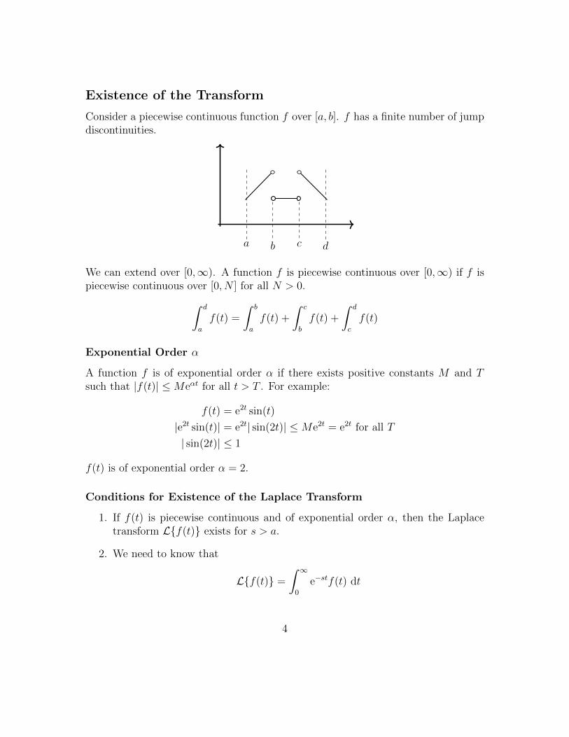
Existence of the Transform

Consider a piecewise continuous function f over [a, b]. f has a finite number of jumpdiscontinuities.

a b c d

We can extend over [0,∞). A function f is piecewise continuous over [0,∞) if f ispiecewise continuous over [0, N ] for all N > 0.∫ d

a

f(t) =

∫ b

a

f(t) +

∫ c

b

f(t) +

∫ d

c

f(t)

Exponential Order α

A function f is of exponential order α if there exists positive constants M and Tsuch that |f(t)| ≤Meαt for all t > T . For example:

f(t) = e2t sin(t)

|e2t sin(t)| = e2t| sin(2t)| ≤Me2t = e2t for all T

| sin(2t)| ≤ 1

f(t) is of exponential order α = 2.

Conditions for Existence of the Laplace Transform

1. If f(t) is piecewise continuous and of exponential order α, then the Laplacetransform Lf(t) exists for s > a.

2. We need to know that

Lf(t) =

∫ ∞0

e−stf(t) dt

4

converges for s > a. We can rewrite it as∫ ∞0

e−stf(t) dt =

∫ T

0

e−stf(t) dt+

∫ ∞T

e−stf(t) dt

where we have |f(t)| ≤Meαt for all t > T . By continuity,∫ T0

e−stf(t) dt exists,so we only need to consider

∫∞T

e−stf(t) dt.∫ ∞T

e−stf(t) dt = limN→∞

∫ N

T

e−stf(t) dt

≤ limN→∞

∫ N

T

Me−steαt dt

= limN→∞

M

∫ N

T

e−(s−α)t dt

= limN→∞

M

[− 1

s− αe−(s−α)t

]NT

= limN→∞

M

[− 1

s− αe−(s−α)N − (− 1

s− αe−(s−α)T )

]=

M

s− αe−(s−α)T <∞

Since M and T are positive constants, this integral converges by the comparison testfor improper integrals.

Properties of the Transform

• Translation in s: If the Laplace transform Lf(t) = F (s) exists, then Leαtf(t) =F (s − a). eαt indicates a translation in the s domain, where we replace s bys− a in the transform of f(t). For example:

Le2t sin(2t) α = 2

Lsin(2t) =2

s2 + 4

Le2t sin(2t) =2

(s− 2)2 + 4

5

Another example:

Le−2t cos(2t) α = −2

Lcos(2t) =s

s2 + 4

Le−2t cos(2t) =s+ 2

(s+ 2)2 + 4

The Laplace Transform of the Derivative

Let f be continuous on [0,∞) and f ′ be piecewise continuous on [0,∞) and both areof exponential order α.

Lf ′(t) =

∫ ∞0

e−stf ′(t) dt

= limN→∞

∫ N

0

e−stf ′(t) dt

u = e−st dv = f ′(t) dt

du = −se−st dt v = f(t)

= limN→∞

[e−stf(t)

]N0

+ limN→∞

s

∫ N

0

e−stf(t) dt

= −f(0) + sF (s)

= sF (s)− f(0)

In summary:

Ly′ = sY (s)− y(0)

Ly′′ = s2Y (s)− sy(0)− y′(0)

Derivatives of the Laplace Transform

Let F (S) = Lf(t). Then for s > a:

Ltnf(t) = (−1)ndnF

dsn

6

For example:

Lt sin(t) n = 1 f(t) = sin(t)

Lsin(t) =1

s2 + 1= F (s)

dF

ds=

d

ds

[1

s2 + 1

]=

(s2 + 1)(0)− 1(2s)

(s2 + 1)2

=−2s

(s2 + 1)2

Lt sin(t) = (−1)1−2s

(s2 + 1)2=

2s

(s2 + 1)2

Another example:

Lte−2t sin(3t) n = 1 f(t) = e−2t sin(3t)

F (s) = Le−2t sin(3t)

Lsin(3t) =3

s2 + 9

Le−2t sin(3t) =3

(s+ 2)2 + 9= F (s)

d

dsF (s) =

0− (3(2(s+ 2)))

((s+ 2)2 + 9)2

=−6(s+ 2)

((s+ 2)2 + 9)2

Lte−2t sin(3t) = (−1)1−6(s+ 2)

((s+ 2)2 + 9)2

=6(s+ 2)

((s+ 2)2 + 9)2

Inverse Laplace Transforms

The Laplace transform maps a function f(t) to a function F (s) = Lf(t). Thetransform has an inverse denoted by:

L−1f(t) = f(t)

7

Consider the following initial value problem:

y′′ − y = −t y(0) = 0 y′(0) = 1

If we apply the Laplace transform to the entire equation:

Ly′′ − y = L−tLy′′ − Ly = −Lt

s2Y (s)− (s)y(0)− y′(0)− Y (s) = − 1

s2

(s2 − 1)Y (s) = − 1

s2+ 1

=−1 + s2

s2

Y (s) =1

s2

L−1Y (s) = L−1 1

s2

t = y(t)

Given F (s), if there exists a function f(t) that is continuous on [0,∞) where Lf(t) =F (s), f(t) is the inverse of F (s). The inverse Laplace transform is a linear operator.Given F1(s), F2(s) and k a constant, the properties of linearity apply:

1. L−1F1(s)± F2(s) = L−1F1(s) ± L−1F2(s)

2. L−1kF1(s)± = kL−1F1

Example

L−1 3

s2 + 9 = L−1 3

s2 + 32

= sin(3t)

L−1 s− 2

(s− 2)2 + 4 = e2t cos(2t)

L−1 1

s− 6 = e6t

8

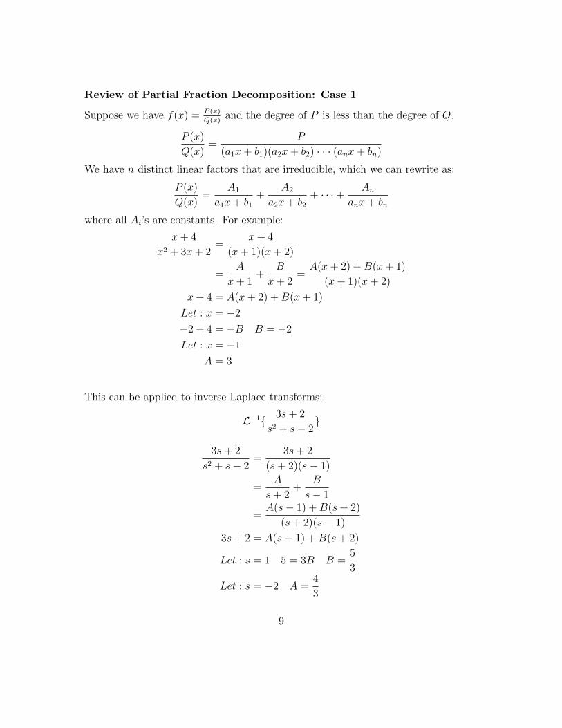
Review of Partial Fraction Decomposition: Case 1

Suppose we have f(x) = P (x)Q(x)

and the degree of P is less than the degree of Q.

P (x)

Q(x)=

P

(a1x+ b1)(a2x+ b2) · · · (anx+ bn)

We have n distinct linear factors that are irreducible, which we can rewrite as:

P (x)

Q(x)=

A1

a1x+ b1+

A2

a2x+ b2+ · · ·+ An

anx+ bn

where all Ai’s are constants. For example:

x+ 4

x2 + 3x+ 2=

x+ 4

(x+ 1)(x+ 2)

=A

x+ 1+

B

x+ 2=A(x+ 2) +B(x+ 1)

(x+ 1)(x+ 2)

x+ 4 = A(x+ 2) +B(x+ 1)

Let : x = −2

−2 + 4 = −B B = −2

Let : x = −1

A = 3

This can be applied to inverse Laplace transforms:

L−1 3s+ 2

s2 + s− 2

3s+ 2

s2 + s− 2=

3s+ 2

(s+ 2)(s− 1)

=A

s+ 2+

B

s− 1

=A(s− 1) +B(s+ 2)

(s+ 2)(s− 1)

3s+ 2 = A(s− 1) +B(s+ 2)

Let : s = 1 5 = 3B B =5

3

Let : s = −2 A =4

3

9

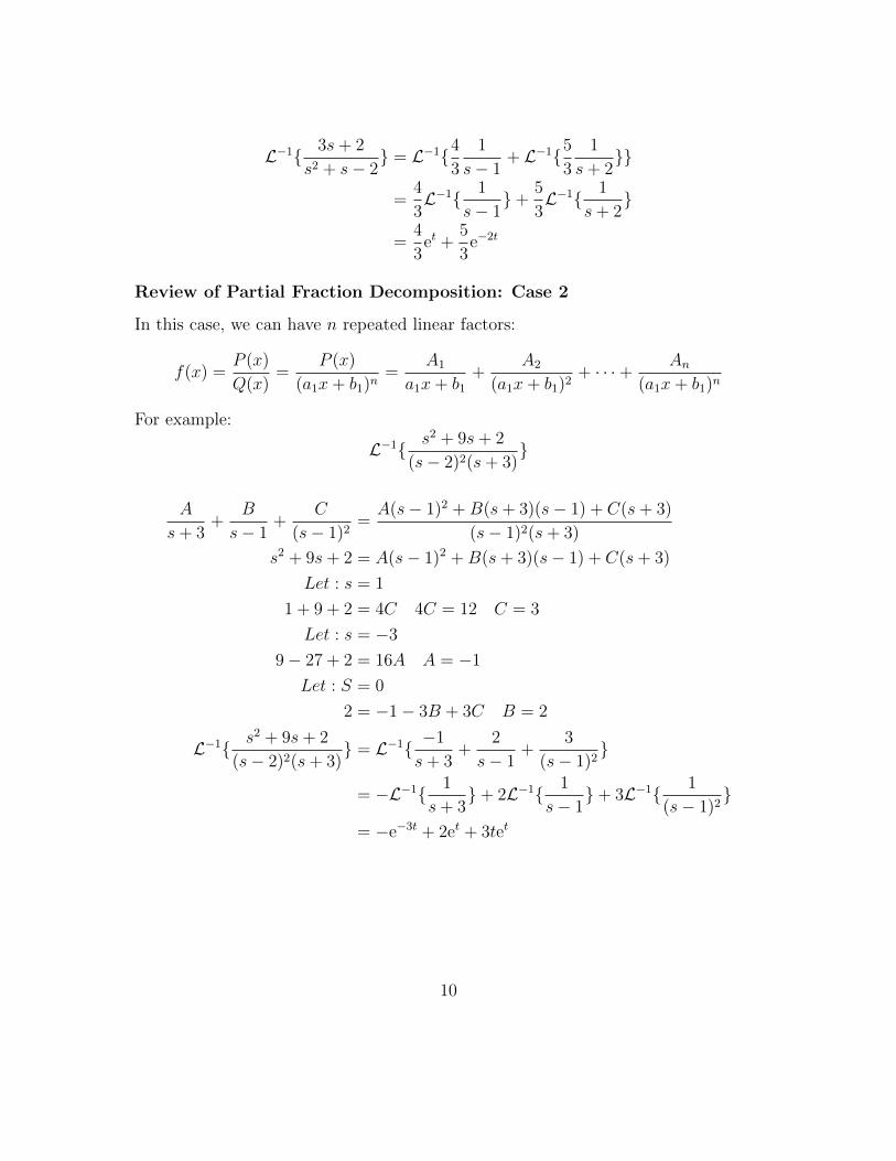
L−1 3s+ 2

s2 + s− 2 = L−14

3

1

s− 1+ L−15

3

1

s+ 2

=4

3L−1 1

s− 1+

5

3L−1 1

s+ 2

=4

3et +

5

3e−2t

Review of Partial Fraction Decomposition: Case 2

In this case, we can have n repeated linear factors:

f(x) =P (x)

Q(x)=

P (x)

(a1x+ b1)n=

A1

a1x+ b1+

A2

(a1x+ b1)2+ · · ·+ An

(a1x+ b1)n

For example:

L−1 s2 + 9s+ 2

(s− 2)2(s+ 3)

A

s+ 3+

B

s− 1+

C

(s− 1)2=A(s− 1)2 +B(s+ 3)(s− 1) + C(s+ 3)

(s− 1)2(s+ 3)

s2 + 9s+ 2 = A(s− 1)2 +B(s+ 3)(s− 1) + C(s+ 3)

Let : s = 1

1 + 9 + 2 = 4C 4C = 12 C = 3

Let : s = −3

9− 27 + 2 = 16A A = −1

Let : S = 0

2 = −1− 3B + 3C B = 2

L−1 s2 + 9s+ 2

(s− 2)2(s+ 3) = L−1 −1

s+ 3+

2

s− 1+

3

(s− 1)2

= −L−1 1

s+ 3+ 2L−1 1

s− 1+ 3L−1 1

(s− 1)2

= −e−3t + 2et + 3tet

10

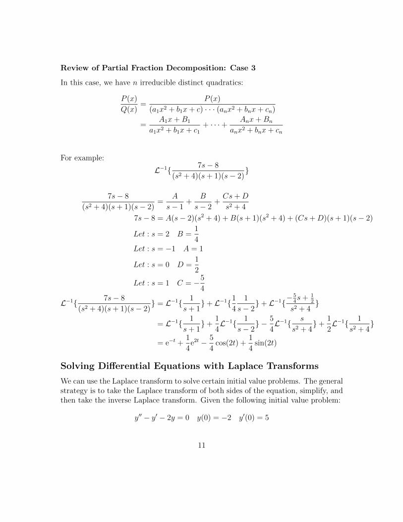
Review of Partial Fraction Decomposition: Case 3

In this case, we have n irreducible distinct quadratics:

P (x)

Q(x)=

P (x)

(a1x2 + b1x+ c) · · · (anx2 + bnx+ cn)

=A1x+B1

a1x2 + b1x+ c1+ · · ·+ Anx+Bn

anx2 + bnx+ cn

For example:

L−1 7s− 8

(s2 + 4)(s+ 1)(s− 2)

7s− 8

(s2 + 4)(s+ 1)(s− 2)=

A

s− 1+

B

s− 2+Cs+D

s2 + 4

7s− 8 = A(s− 2)(s2 + 4) +B(s+ 1)(s2 + 4) + (Cs+D)(s+ 1)(s− 2)

Let : s = 2 B =1

4Let : s = −1 A = 1

Let : s = 0 D =1

2

Let : s = 1 C = −5

4

L−1 7s− 8

(s2 + 4)(s+ 1)(s− 2) = L−1 1

s+ 1+ L−11

4

1

s− 2+ L−1

−54s+ 1

2

s2 + 4

= L−1 1

s+ 1+

1

4L−1 1

s− 2 − 5

4L−1 s

s2 + 4+

1

2L−1 1

s2 + 4

= e−t +1

4e2t − 5

4cos(2t) +

1

4sin(2t)

Solving Differential Equations with Laplace Transforms

We can use the Laplace transform to solve certain initial value problems. The generalstrategy is to take the Laplace transform of both sides of the equation, simplify, andthen take the inverse Laplace transform. Given the following initial value problem:

y′′ − y′ − 2y = 0 y(0) = −2 y′(0) = 5

11

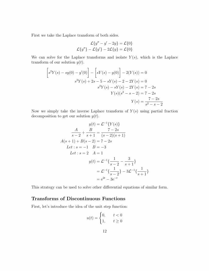
First we take the Laplace transform of both sides.

Ly′′ − y′ − 2y = L0Ly′′ − Ly′ − 2Ly = L0

We can solve for the Laplace transforms and isolate Y (s), which is the Laplacetransform of our solution y(t).[

s2Y (s)− sy(0)− y′(0)

]−[sY (s)− y(0)

]− 2(Y (s)) = 0

s2Y (s) + 2s− 5− sY (s)− 2− 2Y (s) = 0

s2Y (s)− sY (s)− 2Y (s) = 7− 2s

Y (s)(s2 − s− 2) = 7− 2s

Y (s) =7− 2s

s2 − s− 2

Now we simply take the inverse Laplace transform of Y (s) using partial fractiondecomposition to get our solution y(t).

y(t) = L−1Y (s)A

s− 2+

B

s+ 1=

7− 2s

(s− 2)(s+ 1)

A(s+ 1) +B(s− 2) = 7− 2s

Let : s = −1 B = −3

Let : s = 2 A = 1

y(t) = L−1 1

s− 2− 3

s+ 1

= L−1 1

s− 2 − 3L−1 1

s+ 1

= e2t − 3e−t

This strategy can be used to solve other differential equations of similar form.

Transforms of Discontinuous Functions

First, let’s introduce the idea of the unit step function:

u(t) =

0, t < 0

1, t ≥ 0

12

For a > 0:

u(t− a) =

0, t < a

1 t ≥ a

Suppose we have the function:

f(t) =

−1, 0 ≤ t < 3

1, 3 < t < 5

0, t ≥ 5

We can represent this function using the unit step function. The first jump dis-continuity occurs at t = 3, which can be associated with the following unit stepfunction:

u(t− 3) =

0, t < 3

1, t ≥ 3

The jump discontinuity at t = 5 can be associated with the following:

u(t− 5) =

0, t < 5

1, t ≥ 5

Using this, we can rewrite our discontinuous function as the following:

f(t) = −1 + 2u(t− 3)− u(t− 5)

At the boundary on t = 3, the function increases by a value of 2, which becomes thecoefficient for u(t− 3). At the boundary on t = 5, the function decreases by a valueof 1, which becomes the coefficient for u(t− 5).

Example

Let’s consider another example. Suppose now we have the function:

f(t) =

1, 0 < t < 2

t, 2 < t < 3

−1, t ≥ 3

We can represent this function using the unit step function as follows:

f(t) = 1 + (t− 1)u(t− 2)− (t+ 1)u(t− 3)

13

Laplace Transforms of the Unit Step

By definition:

Lu(t− a) =

∫ ∞0

e−stu(t− a) dt

Since this is 0 for t < a by the definition of the unit step function, we can rewritethis as follows: ∫ ∞

0

e−stu(t− a) dt =

∫ ∞a

e−st dt

= limN→∞

∫ N

a

e−st dt

= limN→∞

[− 1

se−st

]Na

= limN→∞

[− 1

se−sN − (−1

se−sa)

]=

e−as

s

For a function y = f(t− a)u(t− a) translated in the t domain:

Lf(t− a)u(t− a) = e−asF (s) = e−asLf(t)

Example

L4u(t− 2) = e−2sL4

= e−2s4

sLsin(t− π)u(t− π) = e−πsLsin(t)

= e−πs1

s2 + 1

The same logic can be applied for inverse transforms:

L−1e−πs 1

(s− 1)2 + 1+ e−2πs

1

s2 = L−1e−πs 1

(s− 1)2 + 1+ L−1e−2πs 1

s2

= et−π sin(t− π)u(t− π) + (t− 2π)u(t− 2π)

14

Example

We can use these techniques to solve differential equations as well. Suppose we have:

y′′ + y = f(t)

f(t) =

0, 0 < t < 2

1, 2 < t < 4

0, 4 < t

y(0) = 1

y′(0) = 0

We can rewrite f(t) using the unit step function.

f(t) = u(t− 2)− u(t− 4)

Now we can use the method of Laplace transforms to solve the differential equation.

y′′ + y = u(t− 2)− u(t− 4)

Ly′′ + y = Lu(t− 2) − Lu(t− 4)Ly′′+ Ly = Lu(t− 2) − Lu(t− 4)[

s2Y (s)− sy(0)− y′(0)

]+ Y (s) =

e−2s

s− e−4s

s

Y (s)(s2 + 1)− s =e−2s

s− e−4s

s

Y (s) =s

s2 + 1+

e−2s

s(s2 + 1)− e−4s

s(s2 + 1)

y(t) = L−1Y (s)

= L−1 s

s2 + 1+ L−1e−2s 1

s(s2 + 1) − L−1e−4s 1

s(s2 + 1)

15

We will need to use partial fraction decomposition to solve these inverse transforms.

1

s(s2 + 1)=A

s+Bs+ C

s2 + 1

=A(s2 + 1) + (Bs+ C)s

s(s2 + 1)

Let : s = 0 A = 1

B = −1

C = 0

y(t) = L−1 s

s2 + 1+ L−1e−2s(1

s− s

(s2 + 1)) − L−1e−4s(1

s− s

(s2 + 1))

= cos(t) + u(t− 2)− cos(t− 2)u(t− 2)− u(t− 4) + cos(t− 4)u(t− 4)

Example

y′ − 4y = sin(t)u(t− 2π) y(0) = 1

y′ − 4y = sin(t− 2π)u(t− 2π)

Ly′ − 4y = Lsin(t− 2π)u(t− 2π)Ly′ − 4Ly = Lsin(t− 2π)u(t− 2π)

sY (s)− 1− 4Y (s) = e−2πs1

s2 + 1

(s− 4)Y (s) = 1 + e−2πs1

s2 + 1

Y (s) =1

s− 4+ e−2πs

1

(s− 4)(s2 + 1)

1

(s− 4)(s2 + 1)=

A

s− 4+Bs+ C

s2 + 1

1 = A(s2 + 1) + (Bs+ C)(s− 4)

A = − 1

17B = − 4

17C =

1

17

16

Y (s) =1

s− 4+ e−2πs

[− 1

17

1

s− 4− 4

17

s

s2 + 1+

1

17

1

s2 + 1

]y(t) = L−1Y (s)

= e4t − 1

17e4(t−2π)u(t− 2π)− 4

17cos(t− 2π)u(t− 2π) +

1

17sin(t− 2π)u(t− 2π)

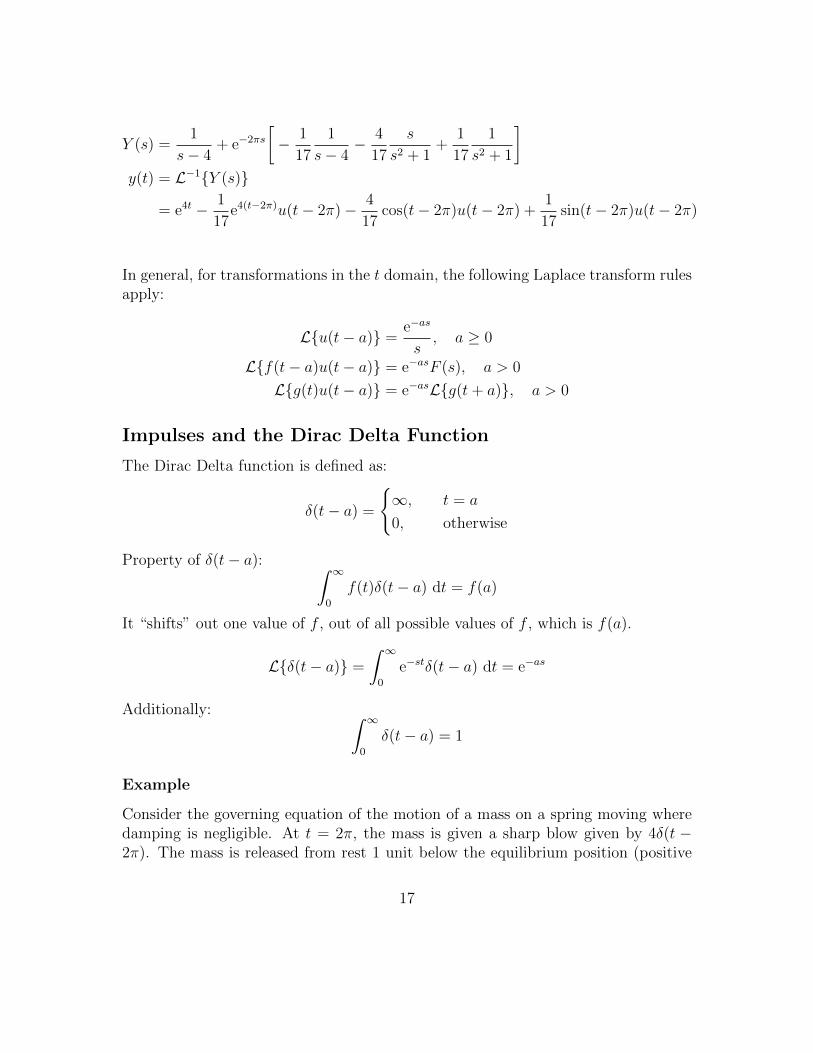
In general, for transformations in the t domain, the following Laplace transform rulesapply:

Lu(t− a) =e−as

s, a ≥ 0

Lf(t− a)u(t− a) = e−asF (s), a > 0

Lg(t)u(t− a) = e−asLg(t+ a), a > 0

Impulses and the Dirac Delta Function

The Dirac Delta function is defined as:

δ(t− a) =

∞, t = a

0, otherwise

Property of δ(t− a): ∫ ∞0

f(t)δ(t− a) dt = f(a)

It “shifts” out one value of f , out of all possible values of f , which is f(a).

Lδ(t− a) =

∫ ∞0

e−stδ(t− a) dt = e−as

Additionally: ∫ ∞0

δ(t− a) = 1

Example

Consider the governing equation of the motion of a mass on a spring moving wheredamping is negligible. At t = 2π, the mass is given a sharp blow given by 4δ(t −2π). The mass is released from rest 1 unit below the equilibrium position (positive

17

direction) with no initial velocity. Find the equation of motion given that the massis 1kg and the spring constant is 1 Newton per meter.

y′′ + y = 4δ(t− 2π)

Ly′′ + y = L4δ(t− 2π)Ly′′+ Ly = 4Lδ(t− 2π)

s2Y (s)− sy(0)− y′(0) + Y (s) = 4e−2πs

s2Y (s)− s− 0 + Y (s) = 4e−2πs

Y (s)(s2 + 1) = s+ 4e−2πs

Y (s) =s

s2 + 1+

4e−2πs

s2 + 1

y(t) = L−1Y (s)

L−1 s

s2 + 1 = cos(t)

4L−1 e−2πs

s2 + 1 = 4L−1e−asF (s)

= 4f(t− a)u(t− a)

a = 2π

F (s) =1

s2 + 1

f(t) = sin(t)

4f(t− a)u(t− a) = 4 sin(t− 2π)u(t− 2π)

= 4 sin(t)u(t− 2π)

y(t) = cos(t) + 4 sin(t)u(t− 2π)

=

cos(t), 0 ≤ t ≤ 2π

cos(t) + 4 sin(t), t > 2π

Convolution

Let f and g be piecewise continuous functions over [0,∞). The convolution of f andg is defined as:

f ∗ g =

∫ t

0

f(t− v)g(v) dv

We call this the convolution intelgral. This operation is commutative, in other words:

g ∗ f = f ∗ g

18

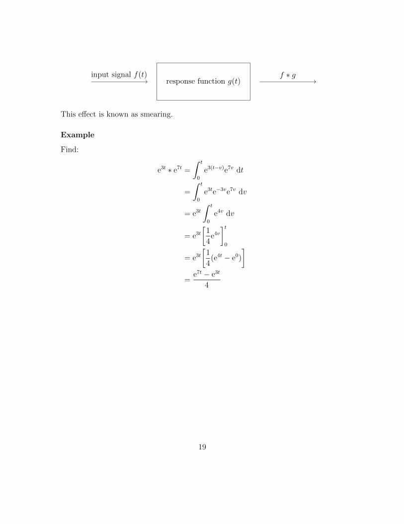
input signal f(t)response function g(t)

f ∗ g

This effect is known as smearing.

Example

Find:

e3t ∗ e7t =

∫ t

0

e3(t−v)e7v dt

=

∫ t

0

e3te−3ve7v dv

= e3t∫ t

0

e4v dv

= e3t[

1

4e4v]t0

= e3t[

1

4(e4t − e0)

]=

e7t − e3t

4

19

Example

Find:

f(t) = et g(t) = e−2t

f ∗ g =

∫ t

0

et−ve−2v dv

=

∫ t

0

ete−ve−2v dv

= et∫ t

0

e−3v dv

= et[− 1

3e−3v

]t0

=et − e−2t

3

The Convolution Theorem

Lf ∗ g = F (s)G(s)

Examples:

Le2t ∗ sin(t) =1

s− 2

1

s2 + 1

L−1 1

s+ 1

1

s+ 2 = e−t ∗ e−2t

=

∫ t

0

e−(t−v)e−2v dv

=

∫ t

0

e−teve−2v dv

= e−t∫ t

0

e−v dv

= e−t[− e−v

]t0

= e−t − e−2t

20

Example

Solve the following integral-differential equation using the method of Laplace trans-forms:

y′ + 6y + 9

∫ t

0

y(v) dv = 1 y(0) = 0∫ t

0

y(v) dv =

∫ t

0

1y(v) dv

= 1 ∗ y(t)

y′ + 6y + 9(1 ∗ y(t)) = 1

Ly′ + 6y + 9(1 ∗ y(t)) = L1

sY (s) + 6Y (s) + 9

[1

sY (s)

]=

1

s

Y (s)(s+ 6 +9

s) =

1

s

Y (s)(s2 + 6s+ 9

s) =

1

s

Y (s) =1

(s+ 3)2

y(t) = L−1 1

(s+ 3)2

= e−3tt

21

Example

Solve the following integral equation.

y(t) = cos(t) +

∫ t

0

e−vy(t− v) dv∫ t

0

e−vy(t− v) dv = e−t ∗ y(t)

y(t) = cos(t) + et ∗ y(t)

Ly(t) = Lcos(t) + et ∗ y(t)

Y (s) =s

s2 + 1+

1

s+ 1Y (s)

Y (s)− 1

s+ 1Y (s) =

s

s2 + 1

(1− 1

s+ 1)Y (s) =

s

s2 + 1

(s+ 1− 1

s+ 1)Y (s) =

s

s2 + 1s

s+ 1Y (s) =

s

s2 + 1

Y (s) =s

s2 + 1

s+ 1

s

=s+ 1

s2 + 1

=s

s2 + 1+

1

s2 + 1

y(t) = L−1Y (s)= cos(t) + sin(t)

22

Example

Solve the following integral equation.

y(t) +

∫ t

0

(t− v)y(v) dv = t2

y(t) + t ∗ y(t) = t2

Ly(t) + t ∗ y(t) = Lt2

Y (s) +1

s2Y (s) =

2

s3

(1 +1

s2)Y (s) =

2

s3

s2 + 1

sY (s) =

2

s3

Y (s) =2

s3s2

s2 + 1

=2

s(s2 + 1)

partial fraction decomposition omitted for brevity

=2

s− 2

s2 + 1

y(t) = L−1Y (s)

= L−12

s − L−1 2

s2 + 1

= 2L−11

s − 2L−1 1

s2 + 1

= 2− 2 cos(t)

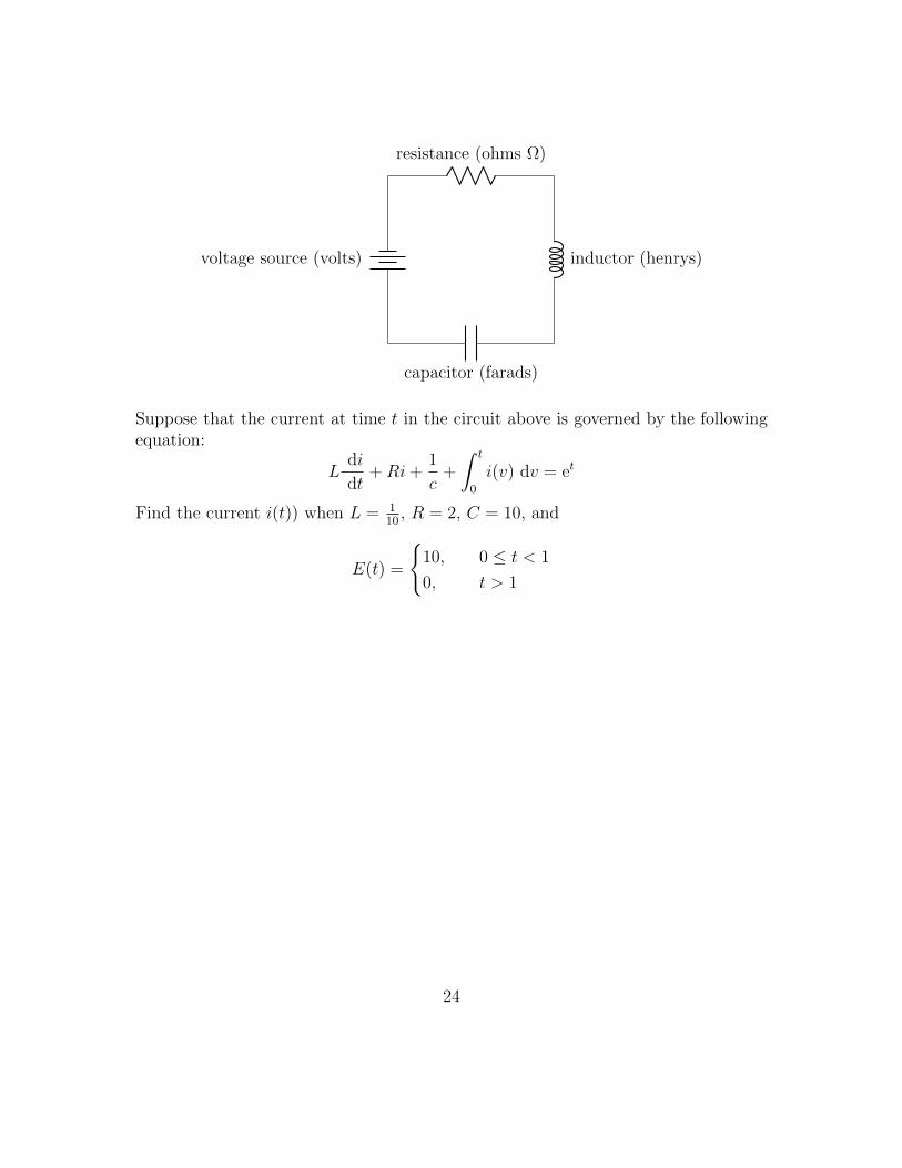
Example

Consider an LRC Series Circuit.

23

voltage source (volts)

resistance (ohms Ω)

inductor (henrys)

capacitor (farads)

Suppose that the current at time t in the circuit above is governed by the followingequation:

Ldi

dt+Ri+

1

c+

∫ t

0

i(v) dv = et

Find the current i(t)) when L = 110

, R = 2, C = 10, and

E(t) =

10, 0 ≤ t < 1

0, t > 1

24

with i(0) = 0.

1

10

di

dt+ 2i(t) + 10

∫ t

0

i(v) dv = E(t)

1

10

di

dt+ 2i(t) + 10

∫ t

0

i(v) dv = 10− 10u(t− 1)

L 1

10

di

dt+ 2i(t) + 10

∫ t

0

i(v) dv = L10− 10u(t− 1)

1

10sI(s) + 2I(s) +

10

sI(s) =

10

s− 10e−s

s

I(s)

[s

10+ 2 +

10

s

]=

10

s− 10

e−2

s

I(s)

[(s+ 10)2

10s

]=

10

s− 10

e−s

s

I(s) =10

s

10s

(s+ 10)2− e−s

[10

s

10s

(s+ 10)2

]=

100

(s+ 10)2− e−s

100

(s+ 10)2

i(t) = L−1I(s)

= L−1 100

(s+ 10)2 − L−1e−s 100

(s+ 10)2

= 100te−10t − 100(t− 1)e−10(t−1)u(t− 1)

You can find all my notes at http://omgimanerd.tech/notes. If you have anyquestions, comments, or concerns, please contact me at alvin@omgimanerd.tech

25