Numerical Methods for Differential Games based

on Partial Differential Equations ∗

M. Falcone

1st June 2005

Abstract

In this paper we present some numerical methods for the solution of two-personszero-sum deterministic differential games. The methods are based on the dynamicprogramming approach. We first solve the Isaacs equation associated to the gameto get an approximate value function and then we use it to reconstruct approximateoptimal feedback controls and optimal trajectories. The approximation schemes alsohave an interesting control interpretation since the time-discrete scheme stems froma dynamic programming principle for the associated discrete time dynamical system.The general framework for convergence results to the value function is the theoryof viscosity solutions. Numerical experiments are presented solving some classicalpursuit-evasion games.

AMS Subject Classification. Primary 65M12; Secondary 49N25, 49L20.

Keywords. Pursuit-evasion games, numerical methods, dynamic programming, Isaacs equation

1 Introduction

In this paper we present a class of numerical methods for two-persons zero-sum determin-istic differential games. These methods are strongly connected to Dynamic Programming(DP in the sequel) for two main reasons. The first is that we solve the Isaacs equationrelated to the game and compute an approximate value function from which we derive allthe informations and the approximations for optimal feedbacks and optimal trajectories.The second is that the schemes are derived from a discrete version of the Dynamic Pro-gramming Principle which gives a nice control interpretation and helps in the analysis ofthe properties of the schemes. This paper is intended to be a tutorial on the subject sowe will present the main ideas and results trying to avoid technicalities. The interestedreader can find all the details and recent developments in the list of references.

It is worth to note that DP is one of the most important tools in the analysis of two-persons zero-sum differential games. It has its roots in the classical work on calculus ofvariations and was applied extensively to optimal control problems by Bellman.

∗Work partially supported by MIUR Project 2003 ”Metodologie Numeriche Avanzate per il Calcolo

Scientifico”. We gratefully acknowledge the technical support given by CASPUR to the development of

this research.

1

The central object of investigation for this method is the value function v(x) of theproblem, which is, roughly speaking, the outcome of the game with initial state x ifthe players behave optimally. In the ’60s many control problems in discrete-time wereinvestigated via the DP method showing that v satisfies a functional equation and that onecan derive from its knowledge optimal controls in feedback form. For discrete-time systems,DP leads to a difference equation for v, we refer the interested reader to the classical books[Ber] and [BeS] for an extended presentation of these results. For continuous-time systems,the situation is more delicate since the DP equation is a nonlinear partial differentialequation (PDE in the sequel) and one has to show first that the equation has a solutionand that this solution is unique, so it coincides with the value function. The main difficultyis the fact that, in general, the value functions of deterministic optimal control problemsand games are not differentiable (they are not even continuous for some problems) sothey are not classical solutions of the DP equation. Moreover, for a deterministic optimalcontrol/game problem the DP equation is of first order and it is well-known that suchequations do not have global classical solutions. In general, one does not even know howto interpret the DP equation at points where v is not differentiable. One way to circumventthe problem is to try to solve the equation explicitly but this can be done only for systemswith low state-space dimensions (typically 1 or 2 dimensions). Isaacs used extensively theDP principle and the first order PDE which is now associated to his name in his book [I] ontwo-persons zero-sum differential games, but he worked mainly on the explicit solution ofseveral examples where the value function is regular except some smooth surfaces. Only atthe beginning of the eighties M.C. Crandall and P.L. Lions [CL] introduced a new notion ofweak solution for a class of first-order PDEs including Isaacs’ equations, and proved theirexistence, uniqueness and stability for the main boundary value problems. These solutionsare called viscosity solutions because they coincide with the limits of the approximationsobtained adding a vanishing second order term to the equation (a vanishing artificialviscosity in physical terms, which explains the name). The theory was reformulated byCrandall, L.C. Evans and Lions [CEL] and P.L. Lions proved in [L] that the value functionsof optimal control problems are viscosity solutions of the corresponding DP equations assoon as they are continuous. The same type of results was obtained for the value function ofsome zero-sum differential games by Barron, Evans, Jensen and Souganidis in [BEJ], [ES],[So] for various definitions of upper and lower value. Independently, Subbotin [Su 1, Su 2]found that the value functions in the Krassovski-Subbotin [KS] sense of some differentialgames satisfy certain inequalities for the directional derivatives which reduce to the Isaacs’equation at points of differentiability. Moreover, he introduced a different notion of weaksolution for first order nonlinear PDEs, the minmax solution. The book [Su 6] presents thistheory with a special emphasis on the solution of differential games which motivated hisstudy and the name for these solutions (since in games the DP equation has a min-maxoperator, see Section 2). It is important to note that several proofs were given of theequivalence of this notion of weak solution with viscosity solutions (see [EI, LS, SuT] sothat nowadays the two theories are essentially unified, cfr.[Su 3, Su 4, Su 6]. The theory ofviscosity solutions has received many contributions in the last twenty years so that it nowcovers several boundary and Cauchy problems for general first and second order nonlinearPDEs. Moreover, the theory has been developed to deal with discontinuous solutionsat least for some classes of Hamilton-Jacobi equations, which include DP equations forcontrol problems (see [Ba 1], [BJ 2], [S 3]). An extensive presentation of the theory of

2

viscosity solutions can be found in the survey paper [CIL] and in the book [Ba 2]. For theapplications to control problems and games the interested reader should refer to the books[FS] and [BCD].

The numerical approximation of viscosity solutions has grown in parallel with theabove mentioned theoretical results and in [CL 2] Crandall and Lions have investigated anumber of monotone schemes proving a general convergence result. As we said, the theoryhas shown to be successful in many fields of application so that numerical schemes arenow available for nonlinear equations arising e.g. in control, games, image processing,phase-transitions, economics. The theory of numerical approximation offers some gen-eral convergence results mainly for first order schemes and for convex Hamiltonians, see[BSo], [LT]. A general results for high-order semi-Lagrangian approximation schemes hasbeen recently proved by Ferretti [Fe]. The approximation of the value function in theframework of viscosity solutions has been investigated by several authors starting fromCapuzzo Dolcetta [CD] and [F 1]. Several convergence results as well as a-priori error es-timates are now available for the approximation of classical control problems and games,see e.g. [BF 1], [BF 2], [CDF], [A 1], [A 2], [BS 3]. The interested reader will find in thesurvey papers [F 1] and [BFS2] a comprehensive presentation of this theory respectivelyfor control problems and games. We will present in the sequel the main results of thisapproach which is based on a discretization in time of the original control/game problemfollowed by a discretization in space which result in a fixed point problem. This approachis natural for control problems since at every discretization we keep the meaning of theapproximate solutions in terms of the control problem and we have a-priori error estimateswhich just depend on the data of the problem and on the discretization steps. Thus thealgorithms based on this approach produce approximate solutions which are close to theexact solution within a given tolerance. Moreover, by the approximate value function onecan easily compute approximate feedback controls and optimal trajectories. For the syn-thesis of feedback controls we have some error estimates in the case of control problems[F 2] but the problem is still open for games. Before starting our presentation let us quoteother numerical approaches related to the approximation of games. The theory of minmaxsolutions has also a numerical counterpart which is based on the construction of general-ized gradients adapted to finite difference operators which approximate the value function.This approach has been developed by the russian school (see [TUU], [PT]) and has alsoproduced an approximation of optimal feedback controls [T]. Another approximation forthe value and for the optimal policies of dynamic zero-sum stochastic games has beenproposed in [TA], [TPA] and it is based on the approximation of the game by a finite stateapproximation (see also [TG 1] for a numerical approximation of zero-sum differentialgames with stopping time). The theory of viability [A] gives a different characterizationof the value function of control/game problems: the value function is the boundary of theviability kernel. This approach is based on set-valued analysis and allows to deal easilywith lower semicontinuous solutions of the DP equation [F]. The numerical counterpartof this approach is based on the approximation of the viability kernel and can be foundin [CQS1] and [CQS2]. Finally, let us mention that other numerical methods based onthe approximation of open-loop control have been proposed. The advantage is of courseto replace the approximation of the DP equation (which can be difficult or impossible tosolve for high-dimensional problems) by a large system of ordinary differential equationsexploiting the necessary conditions for the optimal policy and trajectory. The interested

3

reader can find in [P] a general presentation and in [LBP1], [LBP 2] some examples of theeffectiveness of the method.

This paper is based on the lectures given at the Summer School on ”Differential Gamesand Applications”, held at GERAD, Montreal (June 14-18, 2004) and I want to thank G.Zaccour for his warm hospitality.

The outline of the paper is the following.In Section 1 we briefly present the general framework of the theory of viscosity solutionswhich allows to characterize the value function of control/game problems as the uniquesolution of the DP equation, at the end we give some informations about the extensionto discontinuous viscosity solutions. The first part of this section partly follows the pre-sentation in [B 2]. Section 3 is devoted to the numerical approximation, here we analyzethe time and the space discretization giving the basic results on convergence and errorestimates. A reader already skilled on viscosity solutions can start from there. In Section4 we shortly present the algorithm to compute a numerical synthesis of optimal controlsand give some informations on recent developments. Finally, Section 5 is devoted to thenumerical solution of some classical pursuit-evasion games by the methods presented inthis paper.

2 Dynamic Programming for games and viscosity solutions

Let us consider the nonlinear system

y(t) = f(y(t), a(t), b(t)), t > 0,y(0) = x

(D)

wherey(t) ∈ R

N is the statea( · ) ∈ A is the control of player 1 (player a)

A a : [0,+∞[ → A,measurable (1)

b( · ) ∈ B is the control of player 2 (player b),

B = b : [0,+∞[ → B, measurable , (2)

A,B ⊂ RM are given compact sets. A typical choice is to take as admissible control

function for the two players piecewise constant functions respectively with values in A orB. Assume f is continuous and

|f(x, a, b) − f(y, a, b)| ≤ L |x − y| ∀x, y ∈ RN , a ∈ A, b ∈ B.

By Caratheodory’s theorem the choice of measurable controls guaratees that for any givena( · ) ∈ A and b( · ) ∈ B, there is a unique trajectory of (D) which we will denote byyx(t; a, b). The payoff of the game is

tx(a( · ), b( · )) = min t : yx(t; a, b) ∈ T ≤ +∞, (3)

where T ⊆ RN is a given closed target. Naturally, txa(·), b(·) will be finite only under

additional assumptions on the target and on the dynamics. The two players are opponents

4

since player a wants to minimize the payoff (he is called the pursuer) whereas player bwants to maximize the payoff (he is called the evader). Let us give some examples.

Example 1: Minimum time problemThis is a classical control problem, here we have just one player:

y = a, A = a ∈ R

N : |a| = 1 ,y(0) = x.

Since the maximum speed is 1, tx(a∗) is equal to the length of the optimal trajectoryjoining x and the point yx(tx(a∗)), thus

tx(a∗) = mina∈A

tx(a) = dist(x, T ).

Note that any optimal trajectory is a straight line.

Example 2: Pursuit-Evasion gamesWe have two players, each one controlling its own dynamics

y1 = f1(y1, a), yi ∈ R

N/2, i = 1, 2y2 = f2(y2, b)

(PEG)

The target is

Tε ≡ |y1 − y2| ≤ ε , for ε > 0, or T0 ≡ (y1, y2) : y1 = y2 .

Then, tx(a( · ), b( · )) is the capture time corresponding to the strategies a(·) and b(·).

2.1 Dynamic Programming for a single player

Let us consider first the case of a single player. So in this section we assume B = b which allow us to write the dynamics (D) as

y = f(y, a), t > 0,y(0) = x.

Define the value functionT (x) ≡ inf

a( · )∈Atx(a) .

T ( · ) is the minimum-time function, it is the best possible outcome of the game for playera, as a function of the initial position x of the system.

Definition 2.1 The reachable set is R ≡ x ∈ RN : T (x) < +∞, i.e.it is the set of

starting points from which it is possible to reach the target.

The reachable set depends on the target, on the dynamics and on the set of admissiblecontrols in a rather complicated way, it is not a datum in our problem.

Lemma 1 (Dynamic Programming Principle) For all x ∈ R, 0 ≤ t < T (x) (so thatx /∈ T ),

T (x) = infa( · )∈A

t + T (yx(t; a)) . (DPP)

5

“Proof”The inequality “≤” follows from the intuitive fact that ∀a( · )

T (x) ≤ t + T (yx(t; a)).

The proof of the opposite inequality “≥” is based on the fact that the equality holds ifa( · ) is optimal for x.

To prove rigorously the above inequalities the following two properties of A are crucial:

1. a( · ) ∈ A ⇒ ∀s ∈ R the function t 7→ a(t + s) is in A;

2. a1, a2 ∈ A and

a(t) ≡

a1(t) t ≤ s,a2(t) t > s.

then a( · ) ∈ A, ∀s > 0.

Note that the DPP works for A = piecewise constants functions into A but not forA = continuous functions into A because joining together two continuous controls weare not guaranteed that the resulting control is continuous.

Let us derive the Hamilton-Jacobi-Bellman equation from the DPP. Rewrite (DPP) as

T (x) − infa( · )

T (yx(t; a)) = t

and divide by t > 0,

supa( · )

T (x) − T (yx(t; a))

t

= 1 ∀t < T (x) .

We want to pass to the limit as t → 0+.Assume T is differentiable at x and limt→0+ commute with supa( · ). Then, if yx(0; a)

exists,sup

a( · )∈A−∇T (x) · yx(0, a) = 1,

so that, if limt→0+

a(t) = a0, we get

supa0∈A

−∇T (x) · f(x, a0) = 1 . (HJB)

This is the Hamilton-Jacobi-Bellman partial differential equation associated to the min-imum time problem. It is a first order, fully nonlinear PDE. Note that in (HJB) thesupremum is taken over the A and not on the set of measurable controls A.

Let us define the Hamiltonian,

H1(x, p) ≡ supa∈A

−p · f(x, a) − 1,

we can rewrite (HJB) in short as

H1(x,∇T (x)) = 0 in R \ T .

6

Note that H1(x, ·) is convex since is the sup of linear operators. A natural boundarycondition on ∂T is

T (x) = 0 for x ∈ ∂T

Let us prove that if T is regular then it is a classical solution of (HJB) (i.e.T ∈ C 1(R\T ))and (HJB) is satisfied pointwise).

Proposition 2 If T ( · ) is C1 in a neighborhood of x ∈ R \ T , then T ( · ) satisfies (HJB)at x.

ProofWe first prove the inequality “≤”.Fix a(t) ≡ a0 ∀t, and set yx(t) = yx(t; a). (DPP) gives

T (x) − T (yx(t)) ≤ t ∀ 0 ≤ t < T (x).

We divide by t > 0 and let t → 0+ to get

−∇T (x) · yx(0) ≤ 1,

where yx(0) = f(x, a0) (since a(t) ≡ a0). Then,

−∇T (x) · f(x, a0) ≤ 1 ∀a0 ∈ A

and we getsupa∈A

−∇T (x) · f(x, a) ≤ 1 .

Next we prove the inequality “≥”.Fix ε > 0. For all t ∈ ]0, T (x)[, by (DPP) there exists αε ∈ A such that

T (x) ≥ t + T (yx(t;αε)) − εt ,

which implies

1−ε ≤T (x) − T (yx(t;αε))

t= −

1

t

∫ t

0

∂

∂sT (yx(s;αε)) ds = −

1

t

∫ t

0∇T (yx(s)) · yx(s;αε) ds .

(4)Adding and subtracting the term ∇T (x) · f(yx(s;αε)) by the Lipschitz continuity of f

we get from (4)

1 − ε ≤ −1

t

∫ t

0∇T (x) · f(x, α(s)) ds + o(1) (5)

so for t → 0+, ε → 0+ we finally get

supa∈A

−∇T (x) · f(x, a) ≥ 1 .

Unfortunately T is not regular even for simple dynamics as the following exampleshows. Consider Example 1 where T (x) = dist(x, T ) it is easy to see that T is not

7

differentiable at x if there exist two distinct points of minimal distance. In fact, forN = 1, f(x, a) = a, A = B(0, 1) and

T = ]−∞,−1] ∪ [1,+∞[ .

we haveT (x) = 1 − |x|

which is not differentiable at x = 0. We must observe also that in this example the Bellmanequation is the eikonal equation

|Du(x)| = 1 (6)

which has infinitely many a.e. solutions also when we fix the values on the boundary ∂T ,

u(−1) = u(1) = 0

Also the continuity of T is, in general, not guarateed.Take the previous example and set A = [−1, 0], then we have

T (1) = 0 limx→1

T (x) = 2 (7)

However, the continuity of T ( · ) is equivalent to the property of Small-Time Local Con-trollability (STLC) around T .

Definition 2.2 Assume ∂T smooth. We say that the STLC is satisfied if

∀x ∈ ∂T ∃a ∈ A : f(x, a) · η(x) < 0. (STLC)

where η(x) is the exteriour normal to T at x.

The STLC guarantees that R is an open subset of RN and that

limx→x0

T (x) = +∞, ∀x0 ∈ ∂R

We want to interpret the HJB equation in a “weak sense” so that T ( · ) is a “solution”(non-classical), unique under suitable boundary conditions.

Let’s go back to the proof of Proposition 2.We showed that

1. T (x) − T (yx(t)) ≤ t, ∀t small and T ∈ C1 implies H(x,∇T (x)) ≤ 0;

2. T (x) − T (yx(t)) ≥ t(1 − ε), ∀t, ε small and T ∈ C1 implies H(x,∇T (x)) ≥ 0.

Idea: If φ ∈ C1 and T − φ has a maximum at x then

T (x) − φ(x) ≥ T (yx(t)) − φ(yx(t)) ∀t,

thusφ(x) − φ(yx(t)) ≤ T (x) − T (yx(t)) ≤ t,

so we can replace T by φ in the proof of Proposition 2 and get

H(x,∇φ(x)) ≤ 0 .

8

Similarly, if φ ∈ C1 and T − φ has a minimum at x, then

T (x) − φ(x) ≤ T (yx(t)) − φ(yx(t)), ∀t.

thusφ(x) − φ(yx(t)) ≥ T (x) − T (yx(t)) ≥ t(1 − ε)

and, by the proof of Proposition 2,

H(x,∇φ(x)) ≥ 0 .

Thus, the classical proof can be fixed when T is not C 1 replacing T with a “test function”φ ∈ C1.

Definition 2.3 (Crandall-Evans-Lions [CEL]) Let F : RN × R × R

N → R be contin-uous, Ω ⊆ R

N open. We say that u ∈ C(Ω) is a viscosity subsolution of

F (x, u,∇u) = 0 in Ω

if ∀φ ∈ C1, ∀x0 local maximum point of u − φ,

F (x0, u(x0),∇φ(x0)) ≤ 0.

It is a viscosity supersolution if ∀φ ∈ C1, ∀x0 local minimum point of u − φ,

F (x0, u(x0),∇φ(x0)) ≥ 0.

A viscosity solution is a sub- and supersolution.

Theorem 3 If R\T is open and T ( · ) is continuous, then T ( · ) is a viscosity solution ofthe Hamilton-Jacobi-Bellman equation (HJB).

Proof. The proof is the argument before the definition.

The following result (see e.g. [BCD] for the proof) shows the link between viscosityand classical solutions.

Corollary 4

1. If u is a classical solution of F (x, u,∇u) = 0 in Ω then u is a viscosity solution;

2. if u is a viscosity solution of F (x, u,∇u) = 0 in Ω and if u is differentiable at x0

then the equation is satisfied in the classical sense at x0, i.e.

F (x0, u(x0),∇u(x0)) = 0 .

9

It is clear that the set of viscosity solutions contains that of classical solutions. The mainissue in this theory of weak solutions is to prove uniqueness results. This point is veryimportant also for numerical purposes since the fact that we have a unique solution allowto prove convergence results for the approximation schemes. To this end, let us considerthe Dirichlet boundary value problem

u + H(x,∇u) = 0 in Ωu = g on ∂Ω

(BVP)

and prove a uniqueness result under assumptions on H including Bellman’s HamiltonianH1. This new boundary value problem is connected to (HJB) because the new solution of(BVP) is a rescaling of T . In fact, introducing the new variable

V (x) ≡

1 − e−T (x) if T (x) < +∞, i.e. x ∈ R1 if T (x) = +∞, (x /∈ R)

(8)

it is easy to check that, by the DPP,

V (x) = infa( · )∈A

J(x, a)

where

J(x, a) ≡

∫ tx(a)

0e−t dt .

Moreover, V is a solution of

V + maxa∈A

−∇V · f(x, a) − 1 = 0 in RN \ T

V = 0 on ∂T ,(BVP-B)

which is a special case of (BVP), with H(x, p) = H1(x, p) ≡ maxa∈A−p ·f(x, a)−1 andΩ = T c ≡ R

N \ T .The change of variable (8) is called Kruzkov transformation and has several advantages.

First of all V takes values in [0, 1] whereas T is generally unbounded and this helps in thenumerical approximation. Moreover, one can always reconstruct T and R from V by therelations

T (x) = − log(1 − V (x)), R = x : V (x) < 1 .

Lemma 5 The Mininimum Time Hamiltonian H1 satisfies the “structural condition”

|H(x, p) − H(y, q)| ≤ K(1 + |x|)|p − q| + |q|L |x − y| ∀x, y, p, q, (SH)

where K and L are two positive constants.

Theorem 6 (Crandall-Lions [CL 1]) Assume H satisfies (SH), u,w ∈ BUC(Ω), u sub-solution, w supersolution of v + H(x,∇v) = 0 in Ω (open), u ≤ w on ∂Ω. Then, u ≤ win Ω.

Definition 2.4 We call subsolution (respectively supersolution) of (BVP-B) a subsolution(respectively supersolution) u of the differential equation such that u ≤ 0 on ∂Ω (respec-tively ≥ 0 on ∂Ω).

10

Corollary 7 If the value function V ( · ) ∈ BUC(T c), then V is the maximal subsolutionand the minimal supersolution of (BVP-B) (we say it is the complete solution). Thus Vis the unique viscosity solution.

If the system is STLC around T (i.e. T ( · ) is continuous at each point of ∂T ) thenV ∈ BUC(T c) and we can apply the Corollary.

2.2 Dynamic Programming for games

We now go back to our original problem to develop the same approach. The first questionis: how can we define the value function for the 2-players game ? Certainly it is not

infa∈A

supb∈B

J(x, a, b)

because a would choose his control function with the information of the whole futureresponse of player b to any control function a( · ) and this will give him a big advantage.

A more unbiased information pattern can be modeled by means of the notion of nonan-ticipating strategies (see [EK] and the references therein),

∆ ≡ α : B → A : b(t) = b(t) ∀t ≤ t′ ⇒ α[b](t) = α[b](t) ∀t ≤ t′ , (9)

Γ ≡ β : A → B : a(t) = a(t) ∀t ≤ t′ ⇒ β[a](t) = β[a](t) ∀t ≤ t′ . (10)

The above definition is fair with respect to the two players. In fact, if player a chooses hiscontrol in ∆ he will not be influenced by the future choices of player b (Γ has the samerole for player b). Now we can define the lower value of the game

T (x) ≡ infα∈∆

supb∈B

tx(α[b], b),

orV (x) ≡ inf

α∈∆supb∈B

J(x, α[b], b)

when the payoff is J(x, a, b) =∫ tx(a,b)0 e−t dt.

Similarly the upper value of the game is

T (x) ≡ supβ∈Γ

infa∈A

tx(a, β[a]),

orV (x) ≡ sup

β∈Γinfa∈A

J(x, a, β[a]) .

We say that the game has a value if the upper and lower values coincide, i.e.if T = T orV = V .

Lemma 8 (DPP for games) For all 0 ≤ t < T (x)

T (x) = infα∈∆

supb∈B

t + T (yx(t;α[b], b)) , ∀x ∈ R \ T ,

and

V (x) = infα∈∆

supb∈B

∫ t

0e−s ds + e−tV (yx(t;α[b], b))

, ∀x ∈ T c.

11

The proof is similar to the 1-player case but more technical due to the use of non-anticipating strategies. Note that the upper values T and V satisfy a similar DPP. Let usintroduce the two Hamiltonians for games Isaacs’ Lower Hamiltonian

H(x, p) ≡ minb∈B

maxa∈A

−p · f(x, a, b) − 1 .

Isaacs’ Upper Hamiltonian

H(x, p) ≡ maxa∈A

minb∈B

−p · f(x, a, b) − 1 .

Theorem 9 (Evans-Souganidis [ES] ) 1. If R \ T is open and T ( · ) is continuous,then T ( · ) is a viscosity solution of

H(x,∇T ) = 0 in R \ T . (HJI-L)

2. If V ( · ) is continuous, then it is a viscosity solution of

V + H(x,∇V ) = 0 in T c.

The structural condition (SH) plays an important role for uniqueness.

Lemma 10 Isaacs’ Hamiltonians H, H satisfy the structural condition (SH).

Then Comparison Theorem 6 applies and we get

Theorem 11 If the lower value function V ( · ) ∈ BUC(T c), then V is the complete solu-tion (maximal subsolution and minimal supersolution) of

u + H(x,Du) = 0 in T c,u = 0 on ∂T .

. (BVP-I-L)

Thus V is the unique viscosity solution.

Note that for the upper value functions T and W the same results are valid with H = H.We can give “capturability” conditions on the system ensuring V, V ∈ BUC(T c).

However, those conditions are less studied for games because there are importantpursuit-evasion games with discontinuous value, the games with “barriers” (cfr.[I]). Itis important to note that in general the upper and the lower values are different. However,the Isaacs condition

H(x, p) = H(x, p) ∀x, p, (11)

guarantees that they coincide.

Corollary 12 If V, V ∈ BUC(T c), then

V ≤ V , T ≤ T .

If Isaacs condition holds then V = V and T = T , (i.e.the game has a value).

12

ProofImmediate from the comparison and uniqueness for (BVP-I-L).

For numerical purposes, one can decide to write down an approximation scheme foreither the upper or the lower value using the techniques of the next section. Beforegoing to it, let us give some informations about the characterization of discontinuousvalue functions for games. This is an important issue because discontinuities appear evenin classical pursuit-evasion games (e.g. in the homicidal chauffeur game that we willpresent and solve in Section 5). We will denote by B(Ω) the set of bounded real functionsdefined on Ω. Let us start with a definition which has been successfully applied to convexHamiltonians.

Definition 2.5 (Discontinuous Viscosity Solutions) Let H(x, u, ·) be convex.We define,

u∗(x) = lim infy→x

u(y), u∗(x) = lim supy→x

u(y)

We say that u ∈ B(Ω) is a viscosity solution if ∀φ ∈ C 1(Ω), the following conditions aresatisfied:1. at every local maximum point x0 for u∗ − φ,

H(x0, u∗(x0),∇φ(x0)) ≤ 0.

2. at every local minimum point x0 for u∗ − φ,

H(x0, u∗(x0),∇φ(x0)) ≥ 0.

As we have seen, to obtain uniqueness one should prove that a comparison principle holds,i.e.for every subsolution w and supersolution W we have

w ≤ W

Although this is sufficient to get uniqueness in the convex case the above definition willnot guarantee uniqueness for nonconvex hamiltonians (e.g.min-max Hamiltonians).

Two new definitions have been proposed. Let us denote by S the set of subsolutions ofour equation and by Z the set of supersolutions always satisfying the Dirichlet boundarycondition on ∂Ω.

Definition 2.6 (minmax solutions [Su 6]) u is a minmax solution if there exists twosequences wn ∈ S and Wn ∈ Z such that

wn = Wn = 0 on ∂Ω (12)

wn is continuous on ∂Ω (13)

and limn wn(x) = u(x) = limn Wn(x), x ∈ Ω. (14)

Definition 2.7 (e-solutions, see e.g.[BCD]) u is an e-solution (envelope solution) ifthere exists two non empty subsets

S(u) ⊂ S Z(u) ⊂ Z

13

such that ∀x ∈ Ωu(x) = sup

w∈S(u)w(x) = inf

W∈Z(u)W (x)

By the comparison Lemma there exists a unique e-solution.In fact, if u and v are two e-solutions,

u(x) = supw∈S(u)

w(x) ≤ infW∈Z(v)

W (x) = v(x)

and alsov(x) = sup

w∈S(v)w(x) ≤ inf

W∈Z(u)W (x) = u(x)

It is interesting to note that in our problem the two definitions coincide.

Theorem 13 Under our hypotheses, u is a minmax solution if and only if u is an e-solution.

3 Numerical approximation

We will describe a method to construct approximation schemes for the Isaacs equationwhere we try to keep the essential informations of the game/control problem which isbehind it. In this approach, the numerical approximation of the first order PDE is basedon a time-discretization of the original control problem via discrete DP principle. Then,the functional equation for the time-discrete problem is ”projected” on a grid to derive afinite dimensional fixed point problem. Naturally, one can also choose to construct directlyan approximation scheme for the Isaacs equation based on classical methods for hyper-bolic PDE, e.g.using a Finite Difference (FD) scheme. However this choice is not simplerfrom the point of view of implementation since it is well known that an up-wind correc-tion is needed in the scheme to keep stability and obtain a converging scheme (cfr.[Str]).Moreover, proving convergence of the scheme by only PDE arguments is sometimes morecomplicated. The dynamic programming schemes which we present in this section have abuilt-in up-wind correction and convergence can be proved also using control arguments.

3.1 Time discretization

Let us start by the time discretization of the minimum time problem. The fact that thereis only one player makes easier to describe the scheme and to introduce the basic ideaswhich are behind this approach. In the previous section, we have seen how one can obtainby the Kruzkov change of variable (8) a characterization of the (rescaled) value functionas the unique viscosity solution of (BVP-B). To build the approximation let us choose atime step h = ∆t > 0 for the dynamical system and define the discrete times tm = mh,m ∈ N. We can obtain a discrete dynamical system associated to (D) just using any one-step scheme for the Cauchy problem. A well known example is the explicit Euler schemewhich corresponds to the following discrete dynamical system

xm+1 = xm + hf(xm, am)x0 = x

(Dh)

14

We will denote by yx(n; am) the state at time nh of the discrete time trajectory verifying(Dh). Define the discrete analogue of the reachable set

Rh ≡ x ∈ RN : ∃ a sequence am and m ∈ N such that xm ∈ T (15)

and

nh(am, x) =

+∞ x /∈ Rh

minm ∈ N : xm ∈ T ∀x ∈ Rh(16)

Nh(x) = minam

nh(am, x), (17)

Thus the discrete analogue of the minimum time function T (·) is Nh(·)h.

Lemma 14 (Discrete Dynamic Programming Principle) Let h > 0 be fixed. Forall x ∈ Rh, 0 ≤ n < Nh(x) (so that x /∈ T ),

hNh(x) = infam

hn + Nh(yx(n; am)) . (DDPP)

Sketch of the proof.The ”≤” inequality is easy since hNh is clearly lower than any choice which makes n steps

on the dynamics and then is optimal starting from xn. For the reverse inequality, bydefinition, for every ε > 0 there exists a sequence aε

n such that

hNh(x) > nh(aεm, x) − ε > hn + Nh(yx(n; aε

m)) − ε (18)

Since ε is arbitrary, this concludes proof.

As in the continuous problem, we apply the Kruzkov change of variable

vh(x) = 1 − e−hNh(x). (19)

Note that, by definition, 0 ≤ vh ≤ 1 and vh has constant values on the set of initial pointsx which can be driven to T by the discrete dynamical system in the same number of steps(of constant width h).

Writing the discrete Discrete Dynamic Programming Principle for n = 1, and changingvariable we get the following characterization of vh

vh(x) = S(vh)(x) on RN \ T (HJBh)

vh(x) = 0 on T (BCh)

whereS(vh)(x) ≡ min

a∈A

[e−hvh(x + hf(x, a))

]+ 1 − e−h (20)

In fact, note that x ∈ Rch ≡ R

N \ R implies x + hf(x, a) ∈ Rch so we can easily extend

vh to Rch just defining

vh(x) = 1 on Rch

and get rid of Rh finally setting (HJBh) on RN \ T .

15

Theorem 15 vh is the unique bounded solution of (HJBh) − (BCh).

Sketch of the proof.The proof directly follows from the fact that S defined in (20) is a contraction map in

L∞(RN ). In fact, one can easily prove (see [BF 1] for details) that for every x ∈ RN

|S(u)(x) − S(w)(x)| ≤ e−h‖u − w‖∞, for any u,w ∈ L∞(RN ). (21)

In order to prove an error bound for the approximation we need to introduce someassumptions which are the discrete analogue of the local controllability assumptions ofSection 1. Let us define the δ-neighbourhood of ∂T

Tδ ≡ ∂T + δB(0, 1) , and d(x) ≡ dist (x, ∂T )

We are now able to prove the following upper bounds for our approximations

Lemma 16 Under our assumptions on f and STLC , there exist some positive constantsh, δ such that

vh(x) ≤ C d(x) + h , ∀h < h , x ∈ Tδ

Theorem 17 Let the assumptions of Lemma 16 be satisfied and let T be compact withnonempty interiour.Then, vh converges to v locally uniformly in R

N for h → 0+

Sketch of the proof.Since vh is a discontinuous function we define the two semicontinuous envelopes

v = lim infh→0+

y→x

vh(y), v = lim suph→0+

y→x

vh(y)

Note that v (respectively v) is lower (respectively upper) semicontinuous. The first stepis to show that

1. v is a viscosity subsolution for (HJB)

2. v is a viscosity supersolution for (HJB)

Then, we want show that both the envelopes satisfy the boundary condition on T . In fact,by Lemma 16,

vh(x) ≤ C d(x) + h

which implies

|v| ≤ C d(x) (22)

|v| ≤ C d(x) (23)

16

so we havev = v = 0 on ∂T

Since the two envelopes coincide on ∂T we can apply the comparison theorem for semi-continuous sub and supersolutions in [BP] and obtain

v = v = v on RN .

We now want to prove an error estimate for our discrete time approximation. Let usassume Q is a compact subset of R where the following condition holds:

∃ C0 > 0 : ∀x ∈ Q there is a time optimal control withtotal variation less than C0 bringing the system to T .

(BV)

Theorem 18 ([BF 2]) Let the assumptions of Lemma 16 be verified and let Q be a com-pact subset of R where (BV) holds. Then there exists two positive constants h and C suchthat

|v(x) − vh(x)| ≤ Ch ∀x ∈ Q,h ≤ h (E)

The above results show that the rate of convergence for the scheme based on the Eulerscheme is 1, which is exactly what we expected.

Now let us go back to games. The same time discretization can be written for thedynamics and natural extensions of Nh and vh are easily obtained. The crucial point isto prove that the discrete dynamic programming principle holds true and that the uppervalue of the discrete game is the unique solution in L∞(RN ) of the external Dirichletproblem

vh(x) = S(vh)(x) on RN \ T (HJIh)

vh(x) = 0 on ∂T (BCh)

where the fixed point operator now is

S(vh)(x) ≡ maxb∈B

mina∈A

[e−hvh(x + hf(x, a, b))

]+ 1 − e−h

The next step is to show that the discretization (HJIh)–(BCh) is convergent to the uppervalue of the game. A detailed presentation goes beyond the purposes of this paper, theinterested reader will find these results in [BS 3]. We just give the main convergence resultfor the continuous case.

Theorem 19 Let vh be the solution of (HJIh)–(BCh), Let T be compact with nonemptyinteriour, the assumptions on f be verified, v be continuous.Then, vh converges to v locallyuniformly in R

N for h → 0+.

17

3.2 Space discretization (1 player)

In order to solve the problem numerically we need a (finite) grid so we have to restrict ourproblem to a compact subdomain. A typical choice is to replace the whole space with ahypercube containing T . We consider a triangular mesh of Q made by triangles Sj, j ∈ Jdenoting by k the size of the mesh (this means that k = ∆x ≡ maxjdiam(Sj). Let usjust remark that one can always decide to build a structured grid for Q as is the case for FDschemes, although for dynamic programming schemes this is not compulsory. Moreover,the use of triangles instead of uniform rectangular cells can be a clever and better choicewhen the boundary of T is rather complicated. We will denote by xi, the nodes of themesh (the vertices of the triangles Sj), typically i is a multi-index, i = (i1, . . . , iN ) whereN is the dimension of the state space of the problem. We denote by L the global numberof nodes.

To simplify the presentation let us take a rectangle Q in R2, Q ⊃ T and present the

scheme for N = 2. Moreover, we map the matrix of the values at the nodes (where vi1,i2 isthe value corresponding to the node xi1,i2) on to a vector V of dimension L by the usualrepresentation by rows where the element vi1,i2 goes into Vm for m = (i1 −1)Ncolumns + i2.This ordering allows us to locate the nodes and their values by a single index so from nowon i ∈ I ≡ 1, . . . , L. We will divide the nodes into three subsets, the algorithm willperfom different operations in the three subsets. Let us introduce the sets of indices

IT ≡ i ∈ I : xi ∈ T (24)

I out ≡ i ∈ I : xi + hf(xi, a) /∈ Q∀a ∈ A (25)

I in ≡ i ∈ I : xi + hf(xi, a) ∈ Q (26)

We can describe the fully discrete scheme simply writing (HJBh) at every node of thegrid such that i ∈ Iin adding the boundary conditions on T and on ∂Q (more precisely,on the part of the boundary where the vectorfield points outward for every control). Thefully discrete scheme is

v(xi) = mina∈A

[βv(xi + hf(xi, a)] + 1 − β, for i ∈ Iin (27)

v(xi) = 0 for i ∈ IT (28)

v(xi) = 1 for i ∈ Iout (29)

where β = e−h. Note that the condition on Iout assigns to those nodes a value greater thanthe maximum value inside Q \ T . It is like saying that once the trajectory leaves Q it willnever come back to T (which is obviously false). Nonetheless the condition is reasonablesince we will never get the information that the real trajectory (living in the whole space)can get back to the target unless we compute the solution in a larger domain containingQ. The solution we compute in Q is correct only if Iout is empty, if this is not the case thesolution is correct in a subdomain of Q and is greater than the real solution everywherein Q. This means that the reachable set is approximated from the inside.

We look for a solution of the above problem in the space of piecewise linear functions

W k ≡ w : Q → [0, 1] : w ∈ C(Q),∇w = constant in Sj (30)

18

For any i ∈ Iin, there exists at least one control such that zi(a) ≡ xi + hf(xi, a) ∈ Q.Associated to zi(a) ∈ Q there is a unique vector of coefficients, λi

j(zi(a)), i, j ∈ I such that

0 ≤ λij(a) ≤ 1,

L∑

j=1

λij(zi(a)) = 1 and zi(a) =

L∑

j=1

λij(zi(a))xj

The coefficients λij(zi(a)) are the local (baricentric) coordinates of the point zi(a) with

respect to the vertices of the triangle containing zi(a). The above conditions just say thatz can be written in a unique way as a convex combination of the nodes. Since we are lookingfor a solution in W k, it is important to note that for any w ∈ W k, w(zi(a)) =

∑j λi

jwj

where wj = w(xj), j = 1, . . . , L. For z /∈ Q we set w(z) = 1.Let us define componentwise the operator S : R

L → RL corresponding to the fully

discrete scheme

[S(U)]i ≡

mina∈A

[βΛi(a) · U ] + 1 − β , ∀ i ∈ Iin

0 ∀ i ∈ IT1 ∀ i ∈ Iout

(31)

where Λi(a) ≡ (λi1(zi(a)), . . . , λi

L(zi(a))) The following theorem shows that S has a uniquefixed point.

Theorem 20 The operator S defined in (31) has the following properties:

i) S is monotone, i.e.U ≤ V implies S(U) ≤ S(V );

ii) S : [0, 1]L → [0, 1]L ;

iii) S is a contraction mapping in the max norm ‖W‖∞ = maxi |Wi|,

‖S(U) − S(V )‖∞ ≤ β‖U − V ‖∞

Sketch of the proof.

i) To prove that S is monotone it suffices to show that for U ≤ V ,

S(U)i ≤ S(V )i, for i ∈ Iin.

In fact, for any i ∈ Iin, we have

S(U)i − S(V )i ≤ βΛi(a) · (U − V )

where a is the control where the minimum for S(V ) is achieved. The proof just follows bythe fact that all the λi

j are nonnegative.

ii) Then, for any U ∈ [0, 1]L

1 − β = Si(0) ≤ Si(U) ≤ Si(1) = 1, ∀ i ∈ Iin

19

where 1 ≡ (1, 1, . . . , 1). This concludes the proof.iii). For any i ∈ Iin

Si(U) − Si(V ) ≤ βΛi(a)(U − V )

and ‖Λi(a)‖∞ ≤ 1, ∀ a ∈ A which implies

‖Si(U) − S(V )‖∞ ≤ β‖U − V ‖∞.

Although one can compute the fixed point starting from any initial guess U 0 it is moreefficient to start from an initial guess in the set of discrete supersolutions U +,

U+ ≡ U ∈ [0, 1]L : U ≥ S(U)

This will guarantee monotone convergence. In fact, let us consider the fixed point sequence

Un+1 ≡ S(Un) (32)

Taking U 0 ∈ U+, the monotonicity of S implies

U0 ≥ S(U0) = U1, U1 ≥ U2, U2 ≥ U3 . . .

and Un converges to U ∗ monotonically decreasing by the fixed point argument. A typicalchoice for U 0 ∈ U+ is

U0i =

0 ∀ i ∈ IT1 elsewhere

It is also interesting to remark that in the algorithm the information flows from the targetto the other nodes of the grid. In fact, on the nodes in Q \ T we have U 0

i = 1 but thesevalues immediately decrease in a neighbourhood of T since, by the local controllabilityassumption, the Euler scheme drives them to the target in just one step. At the nextiteration other values, in a larger neighbourhood of T , will decrease due to the samemechanism and so on.

3.3 Fully discrete scheme for games

Let us get back to zero-sum games. Using the change of variable v(x) ≡ 1− e−T (x) we canset the Isaacs equation in R

N obtaining

v(x) + min

b∈Bmaxa∈A

[−f(x, a, b) · ∇v(x)] = 1 in RN \ T

v(x) = 0 for x ∈ ∂T(HJI)

Assume we want to solve the equation in Q, an hypercube in RN . As we have seen, inthe case of a single player we need to impose boundary conditions on ∂Q or, at least, onIout. However, the situation for games is much more complicated. In fact, setting thevalue of the solution outside Q equal to 1 (as in the single player case) will imply thatthe pursuer looses every time the evader drives the dynamics outside Q. On the contrary,setting the value to 0 outside Q will give a great advantage to the pursuer. One way todefine more unbiased boundary conditions is the following. Assume that Q = Q1 ∩ Q2,

20

where Qi, i = 1, 2 are subsets of RN/2 which can be interpreted as the set of constraints

for the i-th player. For example, in R2 we can consider as Q1 a vertical strip and as Q2 an

horizontal strip and compute in the rectangle Q which is the intersection of those strips.According to this construction, we penalize the pursuer if the dynamics exits Q1 and theevader if the dynamics exits Q2. When the dynamics exits Q1 and Q2 we have assigna value, e.g.giving an advantage to one of them (in the following scheme we are givingadvantage to the evader).

The discretization in time and space leads to a fully discrete scheme

w(xi) = maxb

mina

[βw(xi + hf(xi, a, b))] + 1 − β for i ∈ I in (33)

w(xi) = 1 for i ∈ Iout2 (34)

w(xi) = 0 for i ∈ IT ∪ Iout1 (35)

where β ≡ e−h and

Iin = i : xi + hf(xi, a, b) ∈ Q \ T for any a ∈ A, b ∈ B (36)

IT = i : xi ∈ T ∩ Q (37)

Iout1 = i : xi /∈ Q2 (38)

Iout2 = i : xi /∈ Q2 \ Q (39)

Theorem 21 The operator S defined in (33) has the following properties:

i) S is monotone, i.e.U ≤ V implies S(U) ≤ S(V );

ii) S : [0, 1]L → [0, 1]L ;

iii) S is a contraction mapping in the max norm,

‖S(U) − S(V )‖∞ ≤ β‖U − V ‖∞

The proof of the above theorem is a generalization of that of Theorem 20 and can befound in [BFS1].

The above result guarantees that there is a unique fixed point U ∗ for S. Naturally thenumerical solution w will be obtained extending by linear interpolation the values of U ∗

and it will depend on the discretization steps h = ∆t and k = ∆x. Let us state the firstconvergence result for continuous value functions

Theorem 22 Let T be the closure of an open set with Lipschitz boundary, “diam Q →+∞” and v be continuous. Then, for h → 0+ and k

h → 0+, wh,k converges to v locallyuniformly on the compact sets of R

N .

Note that the requirement “diam Q → +∞” is just a technical trick to avoid to dealwith boundary conditions on Q (a similar statement can be written in the whole spacejust working on an infinite mesh). We conclude this section quoting a convergence resultwhich holds also in presence of discontinuities (barriers) for the values function. Let w ε

n

be the sequence generated by the numerical scheme with target Tε = x : d(x, T ) ≤ ε.

21

Theorem 23 For all x there exists the limit

w(x) = limε→0+

n→+∞n≥n(ε)

wεn(x)

and it coincides with the lower value V of the game with target T , i.e.w = V . Convergenceis uniform on every compact set where V is continuous.

Can we know a-priori what is the accuracy of the method in the approximation of the valuefunction? This result is necessary to understand how far we are from the real solutionwhen we compute our approximate solution. To simplify, let us assume that the Lipschitzconstant for f Lf ≤ 1 and that v is Lipschitz continuous. Then,

‖wh,k − v‖∞ ≤ Ch1/2

(1 +

(k

h

)2)

The proof of the above error estimate is rather technical and can be found in [S 4].

4 Approximation of optimal feedback and trajectories

One of the goals of every approximation for control problems and games is to computediscrete synthesis of feedback controls. It is interesting to note that the algorithm proposedand analyzed in the previous section computes an approximate optimal control at everypoint of the grid. Since the numerical solution w has been extended to Q by interpolationwe can also compute an approximate optimal feedback at every point of x ∈ Q, i.e.for thecontrol problem we can define the feedback map F : Q → A. In order to construct thismap, let us introduce the notation

Ik(x, a) ≡ e−hw(x + hf(x, a)) + 1 − e−h. (40)

where we indicate by the index k the fact that the above function also depends on thespace discretization. Note that Ik(x, ·) has a minimum over A, but the minimum pointmay be not unique.We want to construct a selection, e.g. take a strictly convex φ and define

Akx = a ∈ A : Ik

x(x, a) = minA

Ik(x, a) (41)

The selection isa∗x = arg min Ak

xφ(a) (42)

In this way we are able to compute our approximate optimal trajectories, we define thepiecewise constant control

ak(s) = a∗xm,hs ∈ [mh, (m + 1)h[ (43)

where xm,h is the state of the Euler scheme, at the iteration m. Error estimates of theapproximation of feedbacks and optimal trajectories are available for control problems in[BCD] [F 1, F 2].

22

For games, the algorithm computes an approximate optimal control couple (a∗, b∗) atevery point of the grid. Again by w we can also compute an approximate optimal feedbackat every point x ∈ Q.

(a∗(x), b∗(x)) ≡ argminmaxe−hw(x + hf(x, a, b)) + 1 − e−h (44)

If that control is not unique then we can select a unique couple, e.g.minimizing two con-vex functionals. A typical choice is to introduce an inertial criterium to stabilize thetrajectories, i.e.if at step n + 1 the set of optimal couples contains (a∗

n, b∗n) we keep it.We end this section giving some informations on recent developments which we cannot

include in this presentation. Some acceleration methods have been implemented to reducethe amount of floating point operation needed to compute the fixed point: Gauss-Seideliterations, monotone acceleration methods [St] and approximation in policy space [TG 2,St]. Moreover, an effort has been made to reduce the size of the problem by means of thedomain decomposition technique, see [QV] for a general presentation of the method andseveral applications to PDEs. This approach has produced parallel codes for the Isaacsequation [FLM, St, FSt].

5 Numerical experiments

Let us examine some classical games and look at their numerical solutions. We will focusour attention to the accuracy in the approximation of the value function as well as tothe accuracy in the approximation of optimal feedbacks and trajectories. In the previoussections we always assumed that the sets of controls A and B were compact. In thealgorithm and in the numerical tests we have used a discrete finite approximation forthose sets which allows to compute the min-max by comparison. For example, we willconsider the following discrete sets

A =a1 + j

a2 − a1

c − 1

, j = 0, . . . , c − 1;

B =b1 + j

b2 − b1

c − 1

, j = 0, . . . , c − 1;

where [a1, a2] and [b1, b2] represent the control sets respectively for the pursuer P and theevader E. Finally, note that all the value functions represented in the pictures have valuesin [0, 1] because we have computed the fixed point after the Kruzkov change of variable.

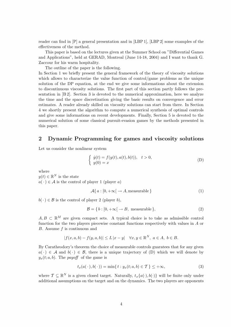
5.1 The Tag-Chase Game

Two boys P and E are running one after the other in the plane R2. P wants to catch E

in minimal time whereas E wants to avoid the capture. Both of them are running withconstant velocity and can change their direction instantaneously. This means that thedynamics of the system is

fP (y, a, b) = vP a fE(y, a, b) = vEb

where vP and vE are two scalars representing the maximum speed for P and E andthe admissible controls are taken in the sets

A = B = B(0, 1).

23

Let us give a more explicit version of the dynamics which is useful for the discretization.Let us denote by (xP , yP ) the position of P and by (xE , yE) the position of E, we canwrite the dynamics as

xP = vP sin θP

yP = vP cos θP

xE = vE sin θE

yE = vE cos θE

(45)

where θP ∈ [a1, a2] ⊆ [−π, π] is the control for P and θE ∈ [b1, b2] ⊆ [−π, π] is the controlfor E, θP and θE are the angles between the y axis and the velocities for P and E (seeFigure 5.1).

We say that E has been captured by P if their distance in the plane is lower than agiven threshold ε > 0. Introducing z ≡ (xP , yP , xE , yE) we can say that the capture occurswhenever z ∈ T where

T ≡z ∈ R

4 :√

(xP − xE)2 + (yP − yE)2 < ε. (46)

The Isaacs equation is set in R4 since every player belongs to R

2. However the resultof the game just depends on the relative positions of P and E, since their dynamics arehomogeneous. In order to reduce the amount of computations needed to compute thevalue function we describe the game in a new coordinate system introducing the variables

x = (xE − xP ) cos θ − (yE − yP ) sin θ (47)

y = (xE − xP ) sin θ − (yE − yP ) cos θ (48)

(49)

The new system (called relative coordinates system) has the origin fixed on the positionof P and moves with this player (see Figure 5.1). Note that the y axis is oriented from Pto E. In the new coordinates the dynamics (45) becomes

˙x = vE sin θE − vP sin θP

˙y = vE cos θE − vP cos θP

(50)

and the target (46) is

T ≡

(x, y) :√

x2 + y2 < ε

.

It is important to note that the above change of variables greatly simplifies the numericalsolution of the problem for three different reasons. The first is that we now solve theIsaacs equation in R

2 and we need a grid of just M 2 nodes instead of M 4 nodes (here Mdenotes the number of nodes in one dimension). The second reason is that we now havea compact target in R

2 whereas the original target (46) is unbounded. This is a majoradvantage since we can choose a fixed rectangular domain Q in R

2 such that it containsT and compute the solution in it. Finally, we get rid of the boundary conditions on ∂Q(see Section 3).

It is easily seen that the game has always a value and that the only interesting case isvP > vE (if the opposite inequality holds true capture is impossible if E plays optimally).In this situation the best strategy for E is to run at maximal velocity in the direction

24

opposite to P along the line passing through the initial positions of P and E. The optimalstrategy for P is to run after E at maximal velocity. The corresponding minimal time ofcapture is

T (xP , yP , xE , yE) =

√(xE − xP )2 + (yE − yP )2

vP − vE

or, in relative coordinates,

T (x, y) =

√x2 + y2

vP − vE.

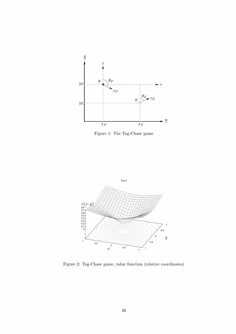
Let us comment some numerical experiments. We have chosen Q = [−1, 1]2

vP = 2, vE = 1, A = B = [−π, π].

Figures 2, 3 correspond to the following discretization

# Nodes ∆t ε # Controls

23 × 23 0.05 0.20 P=41 E=41

The value function is represented in the relative coordinate system, so P is fixed atthe origin and the value at every point is the minimal time of capture (after Kruzkovtransform). As one can see in Figure 2, the behaviour is correct since it correspond toa (rescaled) distance function. The optimal trajectories for the initial positions P =(0.3, 0.3), E = (0.6,−0.3) are represented in Figure 3.

5.2 The Tag-Chase game with constraints on the directions

This game has the dynamics (45). The only difference with respect to the Tag-Chase gameis that now the pursuer P has a constraint on his displacement directions. He can choosehis control in the set θP ∈ [a1, a2] ⊆ [−3/4π, 3/4π]. The evader can still choose his controlas θE ∈ [b1, b2] = [−π, π], i.e.

A = [θ1, θ2] and B = [−π, π].

In the numerical experiment below we have chosen vP = 2, vE = 1, A = [ 34π, 34π] and

B = [−π, π]. As one can see in Figure 4 the time of capture at points which are below theorigin and which cannot be reached by P in a direct way have a value bigger than at thesymmetric points (above the origin). This is clearly due to the fact that P has to zig-zagto those points because the directions pointing directly to them are not allowed (Figure5).

5.3 Zermelo navigation problem

A boat B moves with constant velocity in a river and it can change its direction istanta-neously. The water of the river flows with a velocity σ and the boat tries to reach an islandin the middle of the river (the target) maneuvering against water current. We choose asystem of coordinates such that the velocity of the current is (σ, 0) (see Figure 6). In thenew system, the dynamics of the boat is described by

x = σ + vB cos a,

y = vB sin a,

25

x

y

P

E

PSfrag replacements

hMf

QQ∗

v =?v = 0

v = 1 + Mg

a = 1vB

vP

vE

vr

TBCrRab

xxP xE

xy y

yP

yE

θθ

θP

θE

σ(σ, 0)

Γv(x, y)v(θ, r)

Figure 1: The Tag-Chase game

Test 3

-1-0.5

00.5

1

-1

-0.5

0

0.5

1

00.10.20.30.40.50.60.70.8

PSfrag replacements

hMf

QQ∗

v =?v = 0

v = 1 + Mg

a = 1vB

vP

vE

vr

TBCrRabx

xP

xE

x

y

yyP

yE

θθ

θP

θE

σ(σ, 0)

Γ

v(x, y)

v(θ, r)

Figure 2: Tag-Chase game, value function (relative coordinates)

26

-1

-0.8

-0.6

-0.4

-0.2

0

0.2

0.4

0.6

0.8

1

-1 -0.8 -0.6 -0.4 -0.2 0 0.2 0.4 0.6 0.8 1

Test 3: P=(0.3,0.3) E=(0.6,-0.3)

E

P

PSfrag replacements

hMf

QQ∗

v =?v = 0

v = 1 + Mg

a = 1vB

vP

vE

vr

TBCrRabx

xP

xE

x

y

yyP

yE

θθ

θP

θE

σ(σ, 0)

Γv(x, y)v(θ, r)

Figure 3: Tag-Chase game, optimal trajectoires

Test 4

-1-0.5

00.5

1

-1

-0.5

0

0.5

1

00.10.20.30.40.50.60.70.80.9

PSfrag replacements

hMf

QQ∗

v =?v = 0

v = 1 + Mg

a = 1vB

vP

vE

vr

TBCrRabx

xP

xE

xy

yyP

yE

θθ

θP

θE

σ(σ, 0)

Γ

v(x, y)

v(θ, r)

Figure 4: Constrained Tag-Chase game, value function

27

-2

-1.5

-1

-0.5

0

0.5

1

-1 -0.8 -0.6 -0.4 -0.2 0 0.2 0.4 0.6 0.8 1

Test 4: P=(-0.5,0.8) E=(-0.5,0.0)

P

E

PSfrag replacements

hMf

QQ∗

v =?v = 0

v = 1 + Mg

a = 1vB

vP

vE

vr

TBCrRabx

xP

xE

x

y

yyP

yE

θθ

θP

θE

σ(σ, 0)

Γv(x, y)v(θ, r)

Figure 5: Constrained Tag-Chase game, optimal trajectories

PSfrag replacements

hMf

QQ∗

v =?v = 0

v = 1 + Mg

a = 1

vB

vP

vE

vr

T

B

CrR

a

bx

xP

xE

x

y

yyP

yE

θθ

θP

θE

σ

(σ, 0)

(σ, 0)

Γv(x, y)v(θ, r)

xy

EP

Figure 6: Zermelo navigation problem

28

where a ∈ [−π, π] is the control over the boat direction. Let z(t) =(x(t), y(t)

).

It is easy to see that vB > σ is a sufficient condition for the boat to reach the islandfrom any initial condition in the river. This is not the case if the opposite condition holdstrue (see below). Let us introduce the reachable set

R ≡x0 : ∃t > 0, a(·) ∈ A such that y(t;x0, a(·)) ∈ T

. (51)

This is the set of initial positions from which the boat can reach the island. Let us chooseT =

(0, 0)

, then a simple geometric argument shows that

R =

R2 se vB > σ,(x, y) : x < 0 or x = y = 0

if vB = σ,

(x, y) : x < 0, |y| ≤ −x vB(σ2 − v2B)−

12

if 0 ≤ vB < σ.

(52)

The result is obvious for vB ≥ σ. Now assume 0 < vB < σ. The motion of the boat atevery point is determined by the (vector) sum of its velocity vB and the current velocityσ.

The maximum angle which is allowed to the boat direction is

θ ≡π

2+ arctan

(vB√

σ2 − v2B

)

and the equation of the line with this slope passing from the origin is

y = −xvB√

σ2 − v2B

,

which explains (52). Let us examine the results of two tests. In both tests we have setQ = [−1, 1]2 and the parameters of the discretization are

# Nodes ∆t ε # Controls

80 × 80 0.05 0.10 B=36

In the first test, σ = 1 and vB = 1.4. The value function is presented in Figure 7. SincevB > σ the reachable set is the whole river as predicted by the above argument.

In the second test, σ = 1 and vB = 0.6. As one can see in Figure 8 the reachable setis stricly contained in Q since in this case vB < σ.

5.4 The lady in the lake

A lady E is swimming in a circular lake, she can change her direction istantaneously. Aman P is waiting for her on the shore, he is not able to swim so he can not enter the lakebut he wants to meet her when she leaves the lake. P runs on the shore with a maximumvelocity vP and he can change istantaneously his direction (switching from clockwise tocounterclockwise) (see Figure 9).

Naturally the lady would like to leave the lake at some point but she also wants toavoid the man. We assume that on the ground the velocity of the lady in greater thanthat of the man so that meeting can only occur on the shore, this is the interesting case.

29

Test 1

-1-0.5

00.5

1

-1

-0.5

0

0.5

1

00.10.20.30.40.50.60.70.80.9

1

PSfrag replacements

hMf

QQ∗

v =?v = 0

v = 1 + Mg

a = 1vB

vP

vE

vr

TBCrRabx

xP

xE

xy

yyP

yE

θθ

θP

θE

σ(σ, 0)

Γ

v(x, y)

v(θ, r)

Figure 7: Zermelo problem, value function for σ = 1, vB = 1.4

-1.5-1

-0.50

0.5

-1

-0.5

0

0.5

1

0

0.5

1

PSfrag replacements

hMf

QQ∗

v =?v = 0

v = 1 + Mg

a = 1vB

vP

vE

vr

TBCrRabx

xP

xE

x

y

yyP

yE

θθ

θP

θE

σ(σ, 0)

Γ

v(x, y)

v(θ, r)

Figure 8: Zermelo problem, value function for σ = 1, vB = 0.6

30

PSfrag replacements

hMf

QQ∗

v =?v = 0

v = 1 + Mg

a = 1

vB

vP

vE

vr

TB

C r

R

a

b

xxP

xE

xyy

yP

yE

θ

θθP

θE

σ(σ, 0)

Γv(x, y)v(θ, r)

xy

E

P

Figure 9: The lady in the lake problem

The lady wants to maximize the angular distance PE (measured from the center of thelake) at the time when she exits from the water; naturally P wants to minimize the samedistance.

It is natural to describe the dynamics in polar coordinates. We will denote by θ theangle PCE (where C is the center of the lake) and with r the distance of E from C. Wedenote by R the radius of the lake. The dynamics of the game is

θ = vE sin b

r − vP aR ,

r = vE cos b.

where vE and vP are two scalars representing the maximum velocities of E and P anda ∈ A ≡ [−1, 1] and b ∈ B ≡ [−π, π]. As we made in the tag-chase game we choose asystem of coordinates centered on P . The control a for P is bounded, |A| < 1, and its signcorresponds to the direction followed by P to move along the shore (as usual, + meanscounterclockwise). The control b for E is the angle between the direction chosen by E andthe segment CE, so b ∈ [−π, π].

P (respectively E) wants to minimize (maximize)

∣∣θ(T )∣∣

where T ≡ mint : r(t) = R

is the moment when E exits the lake and θ ∈ [−π, π]. Our

value function will be (in polar coordinates)

v(r, θ) ≡ mina

maxb

∣∣θ(T )∣∣.

Let us now compute v(r, θ) by a geometric argument. Let us assume vP = +1. In therelative coordinate system the E velocity is the (vector) sum vr of two components: thevelocity vector of E in the lake (vE) and a vector vP which is due to the rotation of Paround the lake, this vector is opposite to the direction of P and its modulus is equal tor(t)/R (see Figure 10).

31

P

E

PSfrag replacements

hMf

QQ∗

v =?v = 0

v = 1 + Mg

a = 1vB

vP

vE

vE

vr

TB

C

r

R

a

b

xxP

xE

xyy

yP

yE θ

θθP

θE

σ(σ, 0)

Γv(x, y)v(θ, r)

Figure 10: The lady in the lake, equilibrium strategies

The best strategy for E is to choose b in order to keep vP orthogonal to vr. For anyother choice of b the angle between CE and vr will decrease, i.e. E would move morerapidly toward P which is exactly what the lady wants to avoid. Then, the equilibriumstrategy is b = b∗ where sin(b∗) = RvE/r(t). Note that the above argument to reconstructan optimal strategy for E fails if r(t) < RvE. In fact, in that case E has an angularvelocity greater than P and can always reach a point which is opposite with respect tothe position of P (which means θ(t) = π). Once E reaches the position (θ = π, r = RvP ),her optimal strategy consists in running around (remember, the lady runs faster than theman on the shore). Following [BO] we can obtain the value of the game

∣∣θ(t)∣∣ = π + arccos vE −

1

vE

√1 − v2

E

where we have assumed vP = 1. The above argument is always true for any initial conditionbelonging to the circle or radius RvE. If the initial position of E is outside that circle shecan always enter it swimming in the direction of the center C. It is interesting to notethat from some initial positions outside the circle or radius RvE, E has a better strategy.These initial positions belong to the area which is shadowed in Figure 10. This area isbounded on one side by the lake’s shore and by the two equilibrium trajectories whichstart at the point (θ = π, r = RvE). In this area the optimal trajectories can be obtainedby a direct integration of the Isaacs equation (see [BO], p. 369 for details). Let us set thefollowing values for the parameters: R = 1, vP = 1 and vE = 0.3. For the discretizationwe have used the following values

# Nodes ∆t ε # Controls

40 × 40 0.05 0.10 P=2 E=36

The value function is represented in Figure 11. One can observe that, according to abovediscussion, the time of capture is constant everywhere but in the shadowed area of Figure

32

Test 8

-1-0.5

00.5

1

-1

-0.5

0

0.5

1

00.10.20.30.40.50.60.70.80.9

1

PSfrag replacements

hMf

QQ∗

v =?v = 0

v = 1 + Mg

a = 1vB

vP

vE

vr

TBCrRabx

xP

xE

x

y

yyP

yE

θθ

θP

θE

σ(σ, 0)

Γ

v(x, y)

v(θ, r)

Figure 11: The lady in the lake problem, value function

10. For this problem we do not present optimal trajectories since they are not uniquelydefined. In fact, in this problem there is no running cost (the lady can wait foreverswimming in the center of the lake) so that the lady can always decide to stop her motionalong an equilibrium path, go around everywhere in the lake and get back to the pathwithout affecting the value of the game.

5.5 The Homicidal chauffeur

The presentation of this game follows [FSt]. Let us consider two players (P and E) andthe following dynamics:

xP = vP sin θ,yP = vP cos θ,xE = vE sin b,yE = vE cos b,

θ = RvP

a,

(53)

where a ∈ A ≡ [−1, 1] and b ∈ B ≡ [−π, π] are the two player’s controls. The pursuerP is not free in his movements, he is constrained by a minimum curvature radius R.The target is defined as in the Tag-Chase game. Also in this example we have used thereduced coordinate system (50). We have considered the homicidal chauffeur game whereQ = [−1, 1]2, vP = 1, vE = 0.5, R = 0.2 and the following discretization parameters:

# Nodes ∆t ε # Controls

120 × 120 0.05 0.10 P=36 E=36

Figure 13 shows the value function of the game. Note that when E is in front of P thebehaviour of the two players is analogous to the tag-chase game: in this case, indeed,the constraint on P ’s radius turn does not come into action (Figure 14). However, onthe P sides the value function has two higher lobes. In fact, to reach the correspondingpoints of the domain, the pursuer must first turn around himself to be able to catch Efollowing a straight line (see Figure 15). Finally, behind P there is a region where captureis impossible (v = 1) because the evader has the time to exit Q before the pursuer can catch

33

him. Figure 17 shows a set of optimal trajectories near a barrier in the relative coordinatessystem . Figure 16 is taken from [Me] and shows the optimal trajectories which have beenobtained by analytical methods. One can see that our results are quite accurate since theapproximate trajectories (Figure 17) look very similar to the exact solutions (Figure 16).Moreover, in the numerical approximation the barrier curve is clearly visible: that barriercannot be crossed if both the players behave optimally. It divides the initial positions fromwhich the trajectories point directly to the origin from those corresponding to trajectoriesreaching the origin after a round trip.

6 Conclusions and open problems

As we have seen, the dynamic programming approach can be used to compute the solutionof two-persons zero-sum differential games in low dimension. The accuracy in the recon-struction of the value functions, optimal feedbacks and trajectories is rather satisfactoryalthough it strongly depends on the discretization steps and this has a dramatic impacton the number of floating point operations necessary to compute the solutions. There areseveral open problems from the theoretical as well as from the algorithmic point of view:

1. From the theoretical point of view if would be nice to establish sharp bounds forapproximation of discontinuous value functions in terms of the discretization steps.The extension to high-order schemes also deserves attentions because the use of thisschemes can produce a significative reduction of the grid points required for a givenaccuracy and, on turn, this will reduce the number of floating point operations.Moreover, the accuracy in the reconstruction of optimal feedbacks and trajectoriesis still an open problem.

2. Several points should be investigated to improve the algorithms. The first is todevelop an efficient acceleration method for the fixed point scheme resulting fromthe discretization of the Isaacs equation. Fast Marching Methods have been proposedfor convex Hamiltonians (basically for eikonal type equation) but the extension tonon convex Hamiltonian is still open. Another improvement could be obtained usingadaptive grids which would allow to concentrate the nodes where the singularity ofthe value function appear, (i.e. near the lines of discontinuity of Dv or v).

3. Can the DP approach be extended to other classes of differential games? For ex-ample, one could start from more general non-cooperative games. Once the char-acterization of Nash equilibria and Pareto optima has been derived we could try todevelop numerical schemes for them.

The above program would require strong efforts and several years to be accomplished.

References

[A] J.P. Aubin, Viability Theory, Birkhauser, Boston, 1992.

[A 1] B. Alziary de Roquefort, Jeux differentiels et approximation numerique de fonc-tions valeur, 1re partie: etude theorique, RAIRO Math. Model. Numer. Anal.,25 (1991), 517–533.

34

E

P

x

y

PSfrag replacements

hMf

QQ∗

v =?v = 0

v = 1 + Mg

a = 1vB

vP

vE

vr

TBCr

R a

b

xxP xE

xy

y

yP

yE

θ

θθP

θE

σ(σ, 0)

Γv(x, y)v(θ, r)

Figure 12: The Homicidal Chauffeur problem

Test 5

-1

-0.5

0

0.5

1

-1

-0.5

0

0.5

1

0

0.5

1

PSfrag replacements

hMf

QQ∗

v =?v = 0

v = 1 + Mg

a = 1vB

vP

vE

vr

TBCrRabx

xP

xE

xy

yyP

yE

θθ

θP

θE

σ(σ, 0)

Γ

v(x, y)

v(θ, r)

Figure 13: Homicidal Chauffeur, value function

35

-1

-0.8

-0.6

-0.4

-0.2

0

0.2

0.4

0.6

0.8

1

-1 -0.8 -0.6 -0.4 -0.2 0 0.2 0.4 0.6 0.8 1

Test 5: P=(-0.1,-0.3) E=(0.1,0.3)

P

E

PSfrag replacements

hMf

QQ∗

v =?v = 0

v = 1 + Mg

a = 1vB

vP

vE

vr

TBCrRabx

xP

xE

x

y

yyP

yE

θθ

θP

θE

σ(σ, 0)

Γv(x, y)v(θ, r)

Figure 14: Homicidal Chauffeur, optimal trajectories

-1

-0.8

-0.6

-0.4

-0.2

0

0.2

0.4

0.6

0.8

1

-1 -0.8 -0.6 -0.4 -0.2 0 0.2 0.4 0.6 0.8 1

Test 5: P=(0.0,0.2) E=(0.0,-0.2)

P

E

PSfrag replacements

hMf

QQ∗

v =?v = 0

v = 1 + Mg

a = 1vB

vP

vE

vr

TBCrRabx

xP

xE

x

y

yyP

yE

θθ

θP

θE

σ(σ, 0)

Γv(x, y)v(θ, r)

Figure 15: Homicidal Chauffeur, optimal trajectories

36

PSfrag replacements

hMf

QQ∗

v =?v = 0

v = 1 + Mg

a = 1vB

vP

vE

vr

TBCrRabx

xP

xE

xyy

yP

yE

θθ

θP

θE

σ(σ, 0)

Γv(x, y)v(θ, r)

Figure 16: Homicidal Chauffeur, optimal trajectories (Merz Thesis)

-1

-0.8

-0.6

-0.4

-0.2

0

0.2

0.4

0.6

0.8

1

0 0.1 0.2 0.3 0.4 0.5 0.6 0.7 0.8 0.9 1

Test 5

PSfrag replacements

hMf

QQ∗

v =?v = 0

v = 1 + Mg

a = 1vB

vP

vE

vr

TBCrRabx

xP

xE

x

y

yyP

yE

θθ

θP

θE

σ(σ, 0)

Γv(x, y)v(θ, r)

Figure 17: Homicidal Chauffeur, optimal trajectories (computed)

37

[A 2] B. Alziary de Roquefort, Jeux differentiels et approximation numerique de fonc-tions valuer, 2e partie: etude numerique, RAIRO Math. Model. Numer. Anal.,25 (1991), 535–560.

[AL] B. Alziary de Roquefort, P.L. Lions, A grid refinement method for deterministiccontrol and differential games Math. Models Methods Appl. Sci, 4 (1994), 899-910.

[B 1] M. Bardi. A boundary value problem for the minimum time function, SIAM J.Control Optim., 26 (1989), 776–785.

[B 2] M. Bardi, Viscosity solutions of Isaacs’ equations and existence of a value, Uni-versita di Padova, preprint, 2000.

[BBF] M. Bardi, S. Bottacin, M. Falcone, Convergence of discrete schemes for discontin-uous value functions of pursuit-evasion games, in G.J. Olsder (ed.), ”New Trendsin Dynamic Games and Applications”, Birkhauser, Boston, 1995, 273-304.

[BCD] M. Bardi, I. Capuzzo Dolcetta, Optimal control and viscosity solutions of Hamil-ton-Jacobi-Bellman equations, Birkhauser, 1997.

[BF 1] M. Bardi, M. Falcone, An approximation scheme for the minimum time function,SIAM J. Control Optim., 28 (1990), 950–965.

[BF 2] M. Bardi, M. Falcone, Discrete approximation of the minimal time functionfor systems with regular optimal trajectories, in A. Bensoussan, J.L. Lions (eds.)”Analysis and optimization of systems (Antibes, 1990)”, Lecture Notes in Controland Inform. Sci., vol. 144, Springer, Berlin, 1990, 103–112.

[BFS1] M. Bardi, M. Falcone, P. Soravia, Fully discrete schemes for the value function ofpursuit-evasion games, Advances in dynamic games and applications, T. Basarand A. Haurie eds., Annals of the International Society of Differential Games,Boston: Birkhauser, (1994), vol. 1, 89-105.

[BFS2] M. Bardi, M. Falcone, P. Soravia, Numerical Methods for Pursuit-Evasion Gamesvia Viscosity Solutions, in M. Bardi, T. Parthasarathy and T.E.S. Raghavan (eds.)“Stochastic and differential games: theory and numerical methods”, Annals ofthe International Society of Differential Games, Boston: Birkhauser, (2000) vol.4, 289-303.

[BKS] M. Bardi, S. Koike, P. Soravia, Pursuit-evasion games with state constraints: dy-namic programming and discrete-time approximations, Discrete Contin. Dynam.Systems 6 (2000), 361–380.

[BRP] M. Bardi, T.E.S. Raghavan, T. Parthasarathy (eds.), Stochastic and DifferentialGames: Theory and Numerical Methods, Annals of the International Society ofDifferential Games, Boston: Birkhauser, (2000).

[BS 1] M. Bardi, P. Soravia, A PDE framework for differential games of pursuit-evasiontype, In T. Basar and P. Bernhard, editors, Differential games and applications,Lecture Notes in Control and Information Sciences, 62–71. Springer-Verlag, 1989.

38

[BS 2] M. Bardi, P. Soravia, Hamilton-jacobi equations with singular boundary conditionson a free boundary and applications to differential games, Trans. Amer. Math.Soc. 325 (1991), 205–229.

[BS 3] M. Bardi, P. Soravia, Approximation of differential games of pursuit-evasion bydiscrete-time games, in R.P. Hamalainen and H.K. Ethamo, editors, volume 156of Lecture Notes in Control and Information Sciences, 131–143. Springer-Verlag,1991.

[Ba 1] G. Barles, Discontinuous viscosity solutions of first order Hamilton-Jacobi equa-tions: A guided visit, Nonlinear Anal. T.M.A, 20 (1993), 1123-1134.

[Ba 2] G. Barles, Solutions de viscosite des equations de Hamilton-Jacobi, Mathematicsand Applications, Springer-Verlag, 1994.

[BP] G. Barles, B. Perthame, Discontinuous solutions of deterministic optimal stoppingtime problems, RAIRO Model. Math. Anal. Num., 21 (1987), 557–579.

[BSo] G. Barles, P.E. Souganidis, Convergence of approximation schemes for fully non-linear second order equations, Asymptotic Anal., 4 (1991), 271–283.

[Br] E. N. Barron, Differential games with maximum cost, Nonlinear Anal. T. M. A.,14 (1990), 971–989.

[BEJ] E.N. Barron, L.C. Evans, R. Jensen, Viscosity solutions of Isaacs’ equations anddifferential games with Lipschitz controls, J. Differential Equations, 53 (1984),213–233.

[BJ 2] E. N. Barron, R. Jensen, Optimal control and semicontinuous viscosity solutions,Proc. Amer. Math. Soc., 113:397–402, 1991.

[BO] T. Basar and G. J. Olsder, Dynamic non-cooperative game theory. AcademicPress, New York, 1982.

[Be] L.D. Berkovitz, A survey of recent results in differential games, In T. Basar andP. Bernhard, editors, Differential games and applications, volume 119 of LectureNotes in Control and Information Sciences, pages 35–50. Springer, 1989.

[Ber] D. P. Bertsekas, Dynamic programming. Deterministic and stochastic models,Prentice Hall, Inc., Englewood Cliffs, NJ, 1987.

[BeS] D. P. Bertsekas, S.E. Shreve, Stochastic optimal control. The discrete time case,Mathematics in Science and Engineering, 139. Academic Press, New York-London,1978.

[CD] I. Capuzzo Dolcetta, On a discrete approximation of the Hamilton-Jacobi equationof dynamic programming, Appl. Math. Optim., 10:367–377, 1983.

[CDF] I. Capuzzo Dolcetta, M. Falcone, Viscosity solutions and discrete dynamic pro-gramming, Ann. Inst. H. Poincare Anal. Non Lin., 6 (Supplement):161–183, 1989.

39

[CQS1] P. Cardaliaguet, M. Quincampoix, P. Saint-Pierre, Set valued numerical analysisfor optimal control and differential games, in M. Bardi, T. Parthasarathy andT.E.S. Raghavan (eds.) “Stochastic and differential games: theory and numericalmethods”, Annals of the International Society of Differential Games, Boston:Birkhauser, vol. 4, 1999, 177-247.

[CQS2] P. Cardaliaguet, M. Quincampoix, P. Saint-Pierre, Numerical schemes for discon-tinuous value functions of optimal control. Set-valued analysis in control theory,Set-Valued Anal. 8 (2000), 111–126.

[CEL] M. G. Crandall, L. C. Evans, P. L. Lions, Some properties of viscosity solutionsof Hamilton-Jacobi equations, Trans. Amer. Math. Soc., 282 (1984), 487–502.

[CIL] M. G. Crandall, H. Ishii, P. L. Lions, User’s guide to viscosity solutions of secondorder partial differential equations, Bull. Amer. Math. Soc., 27 (1992) 1–67.

[CL 1] M. G. Crandall, P. L. Lions, Viscosity solutions of Hamilton-Jacobi equations,Trans. Amer. Math. Soc., 277 (1983), 1–42.

[CL 2] M. G. Crandall, P. L. Lions, Two approximations of solutions of Hamilton-Jacobiequations, Math. Comp., 43 (1984), 1–19.

[EK] R.J. Elliott, N.J. Kalton, The existence of value in differential games, Mem.Amer. Math. Soc., 126, 1972.

[EI] L.C. Evans, H. Ishii. Differential games and nonlinear first order PDEs in boundeddomains, Manuscripta Math., 49 (1984), 109–139.

[ES] L. C. Evans, P.E. Souganidis. Differential games and representation formulasfor solutions of Hamilton-Jacobi equations Indiana Univ. Math. J., 33 (1984),773–797.

[F 1] M. Falcone, Numerical solution of Dynamic Programming equations, Appendix Ain the volume M. Bardi and I. Capuzzo Dolcetta, Optimal control and viscositysolutions of Hamilton-Jacobi-Bellman equations, Birkhauser, Boston, 1997.

[F 2] M. Falcone, Some remarks on the synthesis of feedback controls via numericalmethods, in J.L. Menaldi, E. Rofman, A. Sulem (eds), Optimal Control and PartialDifferential Equations, IOS Press, 2001, 456-465.

[FLM] M. Falcone, P. Lanucara, M. Marinucci, Parallel Algorithms for the Isaacs equa-tion, in O. Pourtallier and E. Altman (eds.), ”Advances in Dynamic Gamesand Applications”, Annals of the International Society of Differential Games,Birkhauser (2001), 203-223.

[FSt] M. Falcone, P. Stefani, Advances in Parallel Algorithms for the Isaacs equation,A.S. Nowak and K. Szajowski (eds.), ”Advances in Dynamic Games”, Annals ofthe International Society of Differential Games, Birkhauser (2005), 515-544.

[Fe] R. Ferretti, Convergence of semi-Lagrangian approximations to convex Hamilton-Jacobi equations under (very) large Courant numbers, SIAM J. Numer. Anal., 40(2002), 2240–2253.

40

[FM 1] W.H. Fleming, W.M. McEneaney. Risk sensitive optimal control and differentialgames, volume 184 of Lecture Notes on Control and Information Sciences, pages185–197. Springer, 1992.

[FR] W. H. Fleming. R.W. Rishel, Deterministic and stochastic optimal control.Springer-Verlag, New York, 1975.

[FS] W. H. Fleming, H.M. Soner. Controlled Markov processes and viscosity solutions.Springer Verlag, 1993.

[FSo] W.H. Fleming, P.E. Souganidis, On the existence of value function of two-players,zero-sum differential games. Indiana Univ. Math. J., 38 (1989), 293–314.

[F] H. Frankowska, Lower semicontinuous solutions of Hamilton-Jacobi-Bellmanequations. SIAM J. Control Optim., 31 (1993), 257–272.

[I] R. Isaacs, Differential games, Wiley, New York, 1965.

[Is] H. Ishii, A boundary value problem of the Dirichlet type for Hamilton-Jacobiequations, Ann. Sc. Norm. Sup. Pisa, (IV) 16 (1989), 105–135.

[KS] N.N. Krasovskii, A.I. Subbotin, Game theoretical control problems. Springer,New York 1988.

[LBP1] R. Lachner, M.H. Breitner, H.J. Pesch, Real-time computation of strategies of dif-ferential games with applications to collision avoidance. Variational calculus, op-timal control and applications (Trassenheide, 1996), Internat. Ser. Numer. Math.,124, Birkhuser, Basel, 1998, 281–290.

[LBP2] R.Lachner, M.H. Breitner, H.J. Pesch, Three-dimensional air combat: numericalsolution of complex differential games, in ”New trends in dynamic games andapplications”, Ann. Internat. Soc. Dynam. Games, 3, Birkhuser Boston, Boston,MA, 1995, 165–190.

[LT] C.T. Lin, E. Tadmor, L1-stability and error estimates for approximate Hamilton-Jacobi solutions, Numer. Math. 87 (2001), 701–735.

[L] P. L. Lions, Generalized solutions of Hamilton-Jacobi equations, Pitman, Boston,1982.

[LS] P. L. Lions, P. E. Souganidis, Differential games and directional derivatives ofviscosity solutions of Bellman’s and Isaacs’ equations I and II, SIAM J. ControlOptim., 23 (1985), 566–583 and 24 (1986), 1086–1089.

[Me] A.W. Merz, The Homicidal Chauffeur - a Differential Game, PhD Dissertation,Stanford University, 1971.

[PT] V.S. Patsko, V.L. Turova Numerical study of differential games with the homicidalchauffeur dynamics, Scientific report of the Russian Academy of Science, UralBranch, Ekaterinburg, 2000.

41

[P] H.J. Pesch, Solving optimal control and pursuit-evasion game problems of highcomplexity in Computational optimal control (Munich, 1992), 43–61, Internat.Ser. Numer. Math., 115, Birkhuser, Basel, 1994.

[PB] M.L. Puterman, S.L. Brumelle, On the convergence of policy iteration in station-ary dynamic programming, Mathematics of Operations Research 4 (1979), 60-69.

[QV] A. Quarteroni, A. Valli, Domain decomposition methods for partial differentialequations, Oxford University Press, 1999.

[S 1] P. Soravia, The concept of value in differential games of survival and viscositysolutions of Hamilton-Jacobi equations, Differential Integral Equations, 5 (1992),1049–1068.

[S 2] P. Soravia, Pursuit-evasion problems and viscosity solutions of Isaacs equations,SIAM J. Control Optim., 31 (1993), 604-623.

[S 3] P. Soravia, Discontinuous viscosity solutions to Dirichlet problems for Hamilton-Jacobi equations with convex Hamiltonians, Comm. Partial Diff. Equations, 18(1993), 1493-1514.

[S 4] P. Soravia, Estimates of convergence of fully discrete schemes for the Isaacs equa-tion of pursuit-evasion games via maximum principle, SIAM J. Control Optim.,36 (1998), 1-11.

[St] P. Stefani, Algoritmi paralleli per giochi di fuga-evasione, Tesi di Laurea, Dipar-timento di Matematica, Universita di Roma “La Sapienza”, 1998.

[Str] J.C. Strikwerda, Finite difference schemes for partial differential equations, Chap-man & Hall, 1989.

[So] P. E. Souganidis, Max-min representations and product formulas for the viscositysolutions of Hamilton-Jacobi equations with applications to differential games,Nonlinear Anal. T.M.A., 91985, 217–257.

[Su 1] A. I. Subbotin, A generalization of the basic equation of the theory of differentialgames, Soviet Math. Dokl., 22 (1980), 358–362.

[Su 2] A. I. Subbotin. Generalization of the main equation of differential game theory,J. Optim. Th. Appl. 43 (1984), 103–133.

[Su 3] A. I. Subbotin, Existence and uniqueness results for Hamilton-Jacobi equations,Nonlinear Anal. T.M.A., 16:683–699, 1991.

[Su 4] A. I. Subbotin, Minimax and viscosity solutions of Hamilton-Jacobi equations,Nauka, Moscow, 1991. (In Russian.)

[Su 5] A. I. Subbotin, Discontinuous solutions of a Dirichlet type boundary value prob-lem for first order partial differential equations, Russian J. Numer. Anal. Math.Modelling, 8 (1993), 145–164.

42

[Su 6] A. I. Subbotin, Generalized solutions of first-order PDEs, Birkhauser, Boston,1995.

[SuT] A. I. Subbotin, A.M. Tarasyev, Stability properties of the value function of adifferential game and viscosity solutions of Hamilton-Jacobi equations, Probl.Control Inf. Theory, 15 (1986), 451–463.

[T] A.M. Tarasyev, Control synthesis in grid schemes for Hamilton-Jacobi equa-tions. Optimal control and differential games (Vienna, 1997), Ann. Oper. Res.88 (1999), 337–359.

[TUU] A.M.Tarasyev, A.A. Uspenskiy, V.N. Ushakov, Approximation schemas and finite-difference operators for constructing generalized solutions of Hamilton-Jacobiequations, J. Comput. Systems Sci. Internat. 33 (1995), no. 6, 127–139; translatedfrom Izv. Ross. Akad. Nauk Tekhn. Kibernet. 1994, , no. 3, 173–185(Russian)

[TA] M.M. Tidball, E. Altman, Approximations in dynamic zero-sum games. I, SIAMJ. Control Optim. 34 (1996), no. 1, 311–328.

[TG 1] M.M. Tidball and R.L.V. Gonzalez, Zero sum differential games with stoppingtimes: some results about their numerical resolution, In ”Advances in dynamicgames and applications (Geneva, 1992)”, Ann. Internat. Soc. Dynam. Games, vol.1, Birkhuser, 1994, 106–124.

[TG2] M.M. Tidball and R.L.V. Gonzalez, Fast solution of general nonlinear fixed pointproblems, in ”System modelling and optimization (Zurich, 1991)”, Lecture Notesin Control and Inform. Sci., 180, Springer, Berlin, 1992, 35–44.

[TPA] M.M. Tidball, O. Pourtallier, E. Altman, Approximations in dynamic zero-sumgames. II, SIAM J. Control Optim. 35 (1997), no. 6, 2101–2117.

Author’s addressMaurizio Falcone, Dipartimento di Matematica, Universita di Roma “La Sapienza”, P.Aldo Moro 2, 00185 Roma, e-mail: falcone@mat.uniroma1.it,

43