FOURIER ANALYSIS: LECTURE 17

10 Partial Di↵erential Equations and Fourier methods

The final element of this course is a look at partial di↵erential equations from a Fourier point ofview. For those students taking the 20-point course, this will involve a small amount of overlapwith the lectures on PDEs and special functions.

10.1 Examples of important PDEs

PDEs are very common and important in physics. Here, we will illustrate the methods under studywith three key examples:

The wave equation : r2 =1

c2@2

@t2(10.205)

The di↵usion equation : r2 =1

D

@

@t(10.206)

Schrodinger’s equation :�h2

2mr2 + V = ih

@

@t(10.207)

These are all examples in 3D; for simplicity, we will often consider the 1D analogue, in which (r, t)depends only on x and t, so that r2 is replaced by @2/@x2.

10.1.1 The wave equation

A simple way to see the form of the wave equation is to consider a single plane wave, representedby = exp[i(k · x � !t)]. We have r2 = �k2 , and (@2/@t2) = �!2 . Since !/|k| = c, thisone mode satisfies the wave equation. But a general can be created by superposition of di↵erentwaves (as in Fourier analysis), so also satisfies the equation. Exactly the same reasoning is usedin deriving Schrodinger’s equation. Here we use de Broglie’s relations for momentum and energy:

p = hk; E = h!. (10.208)

Then the nonrelativistic energy-momentum relation, E = p2/2m+V becomes h! = (h2/2m)k2+V .A single wave therefore obeys Schrodinger’s equation, and by superposition and completeness, sodoes a general .

10.1.2 The di↵usion equation

The di↵usion equation is important because it describes how heat and particles get transported,(typically) under conduction. For completeness, here is a derivation – although this is non-examinable in this course.

65

The heat flux density (energy per second crossing unit area of surface) is assumed to be proportionalto the gradient of the temperature (which we will call u, as T is conventionally used for the separatedfunction T (t)):

f(x, t) = ��@u(x, t)@x

, (10.209)

where � is a constant (the thermal conductivity). The minus sign is there because if the temperaturegradient is positive, then heat flows towards negative x.

Now consider a thin slice of width �x from x to x+ �x: there is energy flowing in at the left whichis (per unit area) f(x), and energy is flowing out to the right at a rate f(x+ �x). So in time �t, forunit area of surface, the energy content increases by an amount

�Q = �t [f(x)� f(x+ �x)] ' ��t �x (@f/@x), (10.210)

where we have made a Taylor expansion f(x+ �x) = f(x) + �x (@f/@x) +O([�x]2). This heats thegas. The temperature rise is proportional to the energy added per unit volume,

�u = c�Q

�V(10.211)

where the constant of proportionality c here is called the specific heat capacity. �V = �x is thevolume of the slice (remember it has unit area cross-section). Dividing by �t then gives the di↵usionequation:

�u = �c

@f

@x�x

�

�t1

�V= c�

@2u

@x2

�t ) @u

@t=

@2u

@x2

(10.212)

(for a constant = c�). We often write = 1/D, where D is called the di↵usion coe�cient.

In 3D, this generalises to@u

@t= r2u. (10.213)

The heat transport relation f = ��(@u/@x) takes a vector form f = ��ru, which is just a flowin the direction of maximum temperature gradient, but otherwise identical to the 1D case. Whenthere is a flux-density vector in 3D, the corresponding density, ⇢, obeys the continuity equation,r · f = �@⇢/@t. Since the change in temperature is c times the change in heat density, this givesthe above 3D heat equation.

10.2 Solving PDEs with Fourier methods

The Fourier transform is one example of an integral transform: a general technique for solvingdi↵erential equations.

Transformation of a PDE (e.g. from x to k) often leads to simpler equations (algebraic or ODEtypically) for the integral transform of the unknown function. This is because spatial derivativesturn into factors of ik. Similar behaviour is seen in higher numbers of dimensions. When is asingle Fourier mode

1D :@

@x ! ik ;

@2

@x2

! �k2 (10.214)

3D : r ! ik ; r2 ! �k2 . (10.215)

These simpler equations are then solved and the answer transformed back to give the requiredsolution. This is just the method we used to solve ordinary di↵erential equations, but with the

66

di↵erence that there is still a di↵erential equation to solve in the untransformed variable. Notethat we can choose whether to Fourier transform from x to k, resulting in equations that are stillfunctions of t, or we can transform from t to !, or we can transform both. Both routes should work,but normally we would choose to transform away the higher derivative (e.g. the spatial derivative,for the di↵usion equation).

The FT method works best for infinite systems. In subsequent lectures, we will see how Fourierseries are better able to incorporate boundary conditions.

10.2.1 Example: the di↵usion equation

As an example, we’ll solve the di↵usion equation for an infinite system.

@2n(x, t)

@x2

=1

D

@n(x, t)

@t. (10.216)

The di↵usion coe�cient D is assumed to be independent of position. This is important, otherwisethe FT method is not so useful. The procedure is as follows:

• FT each side:

– Multiply both sides by e�ikx

– Integrate over the full range �1 < x < 1.

– Write the (spatial) FT of n(x, t) as n(k, t)

• Pull the temporal derivative outside the integral over x

• Use Eqn. (3.33) with p = 2 to get:

(ik)2n(k, t) =1

D

@n(k, t)

@t(10.217)

• This is true for each value of k (k is a continuous variable). This is a partial di↵erentialequation, but let us for now fix k, so we have a simple ODE involving a time derivative, andwe note that d(ln n) = dn/n, so we need to solve

d ln n

dt= �k2D. (10.218)

Its solution is ln n(k, t) = �k2Dt + constant. Note that the constant can be di↵erent fordi↵erent values of k, so the general solution is

n(k, t) = n0

(k) e�Dk

2t. (10.219)

where n0

(k) ⌘ n(k, t = 0), to be determined by the initial conditions.

• The answer (i.e. general solution) comes via an inverse FT:

n(x, t) =

Z 1

�1

dk

2⇡n(k, t) eikx =

Z 1

�1

dk

2⇡n0

(k) eikx�Dk

2t . (10.220)

67

n(x,t)

x

increasing time

Figure 10.18: Variation of concentration with distance x at various di↵usion times.

SPECIFIC EXAMPLE: We add a small drop of ink to a large tank of water (assumed 1-dimensional). We want to find the density of ink as a function of space and time, n(x, t).

Initially, all the ink (S particles) is concentrated at one point (call it the origin):

n(x, t = 0) = S �(x) (10.221)

implying (using the sifting property of the Dirac delta function),

n0

(k) ⌘ n(k, 0) =

Z 1

�1dx n(x, t = 0) e�ikx =

Z 1

�1dx �(x) e�ikx = S. (10.222)

Putting this into Eqn. (10.220) we get:

n(x, t) =

Z 1

�1

dk

2⇡n(k, t) eikx =

Z 1

�1

dk

2⇡n0

(k) eikx�Dk

2t

=

Z 1

�1

dk

2⇡S eikx�Dk

2t =

Sp2⇡

p2Dt

e�x

2/(4Dt) . (10.223)

(we used the ‘completing the square’ trick that we previously used to FT the Gaussian). Comparethis with the usual expression for a Gaussian,

1p2⇡�

exp

✓

� x2

2�2

◆

(10.224)

and identify the width � withp2Dt.

So, the ink spreads out with concentration described by a normalized Gaussian centred on the originwith width � =

p2Dt. The important features are:

• normalized: there are always S particles in total at every value of t

• centred on the origin: where we placed the initial drop

• width � =p2Dt: gets broader as time increases

68

– � /pt: characteristic of random walk (‘stochastic’) process

– � /pD: if we increase the di↵usion constant D, the ink spreads out more quickly.

The solution n(x, t) is sketched for various t in Fig. 10.18.

FOURIER ANALYSIS: LECTURE 18

10.3 Fourier solution of the wave equation

One is used to thinking of solutions to the wave equation being sinusoidal, but they don’t have tobe. We can use Fourier Transforms to show this rather elegantly, applying a partial FT (x ! k,but keeping t as is).

The wave equation is

c2@2u(x, t)

@x2

=@2u(x, t)

@t2(10.225)

where c is the wave speed. We Fourier Transform w.r.t. x to get u(k, t) (note the arguments),remembering that the FT of @2/@x2 is �k2:

� c2k2u(k, t) =@2u(k, t)

@t2. (10.226)

This is a harmonic equation for u(k, t), with solution

u(k, t) = Ae�ikct +Beikct (10.227)

However, because the derivatives are partial derivatives, the ‘constants’ A and B can be functionsof k. Let us write these arbitrary functions as f(k) and g(k), i.e.

u(k, t) = f(k)e�ikct + g(k)eikct. (10.228)

We now invert the transform, to give

u(x, t) =

Z 1

�1

dk

2⇡

h

f(k)e�ikct + g(k)eikcti

eikx

=

Z 1

�1

dk

2⇡f(k)eik(x�ct) +

Z 1

�1

dk

2⇡g(k)eik(x+ct)

= f(x� ct) + g(x+ ct)

and f and g are arbitrary functions.

10.4 Fourier solution of the Schrodinger equation in 2D

Consider the time-dependent Schrodinger equation in 2D, for a particle trapped in a (zero) potential2D square well with infinite potentials on walls at x = 0, L, y = 0, L:

� h2

2mr2 (x, t) = ih

@ (x, t)

@t. (10.229)

69

For example, let us perform a FT with respect to x. r2 ! �k.k = �k2 = �(k2

x

+ k2

y

), so

h2k2

2m (k, t) = ih

@ (k, t)

@t. (10.230)

We can integrate this with an integrating factor:

(k, t) = (k, 0)e�i

hk

2

2m t. (10.231)

The time-dependence of the wave is e�i!t, or, in terms of energy E = h!, e�iEt/h, where

E =h2k2

2m. (10.232)

If the particle is trapped in the box, then the wavefunction must be zero on the boundaries, sothe wavelength in the x direction must be �

x

= 2L, L, 2L/3, . . . i.e. 2L/m for q = 1, 2, 3, . . ., orwavenumbers of k

x

= 2⇡/�x

= q⇡/L. Similarly, ky

= r⇡/L for r = 1, 2, . . ..

So the wavefunction is a superposition of modes of the form

(x, t) = A sin⇣q⇡x

L

⌘

sin⇣r⇡y

L

⌘

e�iEt/h (10.233)

for integers q, r. A is a normalization constant to ensure thatR R

| 2| dx dy = 1.

Each mode has an energy

E =h2k2

2m=

h2⇡2(q2 + r2)

2mL2

. (10.234)

For a square well, the energy levels are degenerate – di↵erent combinations of q and r give the sameenergy level.

11 Separation of Variables

We now contrast the approach of Fourier transforming the equations with another standard tech-nique. If we have a partial di↵erential equation for a function which depends on several variables,e.g. u(x, y, z, t), then we can attempt to find a solution which is separable in the variables:

u(x, y, z, t) = X(x)Y (y)Z(z)T (t) (11.235)

where X, Y, Z, T are some functions of their arguments, and we try to work out what these functionsare. Examples of separable functions are xyz2e�t, x2 sin(y)(1 + z2)t, but not (x2 + y2)zt. Not allPDEs have separable solutions, but many physically important examples do.

Let us consider the one-dimensional wave equation (so we have only x and t as variables) as anexample:

@2u

@x2

=1

c2@2u

@t2. (11.236)

We try a solution u(x, t) = X(x)T (t):

@2(XT )

@x2

=1

c2@2(XT )

@t2. (11.237)

Now notice that on the left hand side, T is not a function of x, so can come outside the derivative,and also, since X is a function of x only, the partial derivative with respect to x is the same as the

70

ordinary derivative. A similar argument holds on the right hand side, where X is not a function oft, so

Td2X

dx2

=X

c2d2T

dt2. (11.238)

The trick here is to divide by XT , to get

1

X

d2X

dx2

=1

c2T

d2T

dt2. (11.239)

Now, the left hand side is not a function of t (only of x), whereas the right hand side is not afunction of x (only of t). The only way these two independent quantities can be equal for all t andx is if they are both constant. The constant is called the separation constant, and let us call it �k2.(Note that we aren’t sure at this point that the separation constant is negative; if it turns out it ispositive, we’ll come back and call it k2, or, alternatively, let k be imaginary). Hence the equationfor X is (multiplying by X)

d2X

dx2

= �k2X. (11.240)

You know the solution to this:

X(x) = A exp(ikx) + B exp(�ikx) (11.241)

for constants A and B (alternatively, we can write X as a sum of sines and cosines).

The equation for T is1

c2d2T

dt2= �k2T (11.242)

which has solutionT (t) = C exp(i!t) +D exp(�i!t) (11.243)

where ! = ck. If we take in particular B = C = 0 and A = D = 1, we have a solution

u(x, t) = exp[i(kx� !t)] (11.244)

which we recognise as a sinusoidal wave travelling in the +x direction. In general, we will get amixture of this and exp[i(kx+!t)], which is a sinusoidal wave travelling in the negative x direction.We will also get the same exponentials with the opposite sign in the exponent. These could becombined into

u(x, t) = A sin[(kx� !t) + ↵] + B sin[(kx� !t) + �], (11.245)

which is a mixture of waves travelling in the two directions, with di↵erent phases.

IMPORTANT: Notice that we can add together any number of solutions with di↵erentvalues of the separation constant �k2, and we will still satisfy the equation. This meansthat the full solution can be a more complicated non-periodic function, just as Fourier transformsallow us to express a general function as a superposition of periodic modes. In this case (as we sawabove), the general solution of the 1D wave equation is

u(x, t) = f(x� ct) + g(x+ ct), (11.246)

for any (twice-di↵erentiable) functions f and g.

In general to find which of the many solutions are possible in a given situation, we need to specifywhat the boundary conditions are for the problem, i.e. what restrictions are there on the solutionat (for example) fixed values of x, or t. e.g. if the solution has to be periodic in x, we will have

71

0

2

4

6

x

0

1

2

3

t

-1.0

-0.5

0.0

0.5

1.0

T

0

2

4

6

x

0

1

2

3

t

-1.0

-0.5

0.0

0.5

1.0

T

Figure 11.19: Contrasting the travelling-wave and standing-wave solutions to the wave equation.

exactly the same restrictions on k as in Fourier analysis. Note that the boundary conditions usuallydetermine the solution.

Here is another example. If we require that u is zero at two boundaries x = (0, ⇡), and that att = 0 the solution is a sin wave, u(x, 0) = sin(3x), then the solution is u(x, t) = sin(3x) cos(3ct).This is a standing wave, which does not propagate, just varies its amplitude with time.

Note that we can write the standing wave solution as a superposition of waves travelling in oppositedirections (with ck = !):

sin(kx) cos(!t) =1

2i(eikx � e�ikx)

1

2(ei!t + e�i!t)

=1

4i

⇥

ei(kx+!t) + ei(kx�!t) � e�i(kx�!t) � e�i(kx+!t)

⇤

=1

2[sin(kx+ !t) + sin(kx� !t)] . (11.247)

FOURIER ANALYSIS: LECTURE 19

11.1 Solving the di↵usion equation via separation of variables

Let us now try to solve the di↵usion equation in 1D:

@2u

@x2

=1

@u

@t. (11.248)

We wish to find a solution with u ! 0 as t ! 1. We try separating variables, u(x, t) = X(x)T (t),to find

1

X

d2X

dx2

=1

T

dT

dt= ��2 (11.249)

where we have written the separation constant as ��2. The equation for X is the same as we hadbefore. This time, let us write the solution as sines and cosines:

X(x) = A sin(�x) + B cos(�x). (11.250)

72

The equation for T isdT

dt= ��2T, (11.251)

ord lnT

dt= ��2 (11.252)

which has solutionT (t) = C exp(��2t) (11.253)

so we have a separable solution (absorbing the constant C into A and B)

u(x, t) = [A sin(�x) + B cos(�x)] exp(��2t), (11.254)

This tends to zero as t ! 1 provided �2 > 0. This justifies our implicit assumption that �2 > 0– otherwise we would have an unphysical diverging solution, which would not satisfy the boundarycondition that u ! 0 as t ! 1.

Note that we can add in solutions with di↵erent �, and as usual the full solution will depend onthe initial conditions. This begins to look like Fourier analysis. We certainly need to add at leasta constant in order to make the solution physically sensible: as written, it allows for negativetemperatures. But we can always add a constant to any solution of the di↵usion equation; so whenwe speak of a boundary condition involving u = 0, this really means the temperature is at someuniform average value, which we do not need to specify.

11.2 Separation of variables with several dimensions

As a last example of solving equations via separation of variables, let us consider a more complicatedsituation, where we have 2 space dimensions, and time. Consider an infinite square column of sideL which is initially (at t = 0) at zero temperature, u(x, y, t = 0) = 0. We ignore z as by symmetrythere is no heat flowing along this direction. At t = 0 it is immersed in a heat bath at temperatureT0

. We need to solve the heat equation

r2u =1

@u

@t, (11.255)

and we will look for separable solutions in the following form:

u(x, y, z, t) = T0

+X(x)Y (y)T (t). (11.256)

We do this because this will make it easier to absorb the boundary conditions. Although u = 0throughout the block initially, it is u = T

0

at the surface of the block (at all times). Thus as written,XY T = 0 on the surface of the block at t = 0, which is a simpler boundary condition. We didn’thave to choose this form, but it makes the working simpler. In any case, the di↵erential equationis independent of T

0

:

Y Td2X

d2x+XT

d2Y

d2y� XY Z

dT

dt= 0 (11.257)

Dividing by XY T ,1

X

d2X

d2x+

1

Y

d2Y

d2y� 1

T

dT

dt= 0 (11.258)

Since the first term is not a function of y, t, and the second is not a function of x, t etc, we concludethat all the terms must be constant. e.g.

1

T

dT

dt= �� ) T (t) / e��t. (11.259)

73

We next find the equation for X, by isolating terms which depend on x only:

1

X

d2X

d2x= � 1

Y

d2Y

d2y� � = �k2

x

= constant (11.260)

(the l.h.s. is not a function of y, z, the Y terms is not a function of x, hence they must be equal toanother constant).

d2X

d2x= �k2

x

X ) X(x) = Aeikxx +Be�ik

x

x (11.261)

and similarly for Y – except that the equivalent wavenumber ky

must satisfy k2

x

+ k2

y

= �, fromequation (11.260).

Now, as stated above, the terms we calculate here must be zero on the boundaries at x = 0, L,y = 0, L. Hence the solutions for X and Y must be sinusoidal, with the correct period, e.g.

X(x) / sin⇣m⇡x

L

⌘

(11.262)

for any integer m. Similarly for Y . So a separable solution is

u(x, y, t) = T0

+ Cmn

sin⇣m⇡x

L

⌘

sin⇣n⇡y

L

⌘

e��

mn

t (11.263)

where

�mn

=⇡2

L2

(m2 + n2). (11.264)

Here we have identified the separation constants explicitly with the integers m,n, rewriting � =k2

x

+ k2

y

.

Now we can add the separable solutions:

u(x, y, t) = T0

+1X

m,n=0

Cmn

sin⇣m⇡x

L

⌘

sin⇣n⇡y

L

⌘

e��

mn

t. (11.265)

All that remains is to determine the constants Cmn

. We use the initial condition that inside thevolume u = 0 when t = 0 (when the exponential term is unity), so

1X

m,n=0

Cmn

sin⇣m⇡x

L

⌘

sin⇣n⇡y

L

⌘

= �T0

. (11.266)

This looks very much like a Fourier Series, and we can use the same trick of the orthogonality of thesin functions. Multiply by sin(m0⇡x/L) and integrate with respect to x, giving 0 unless m = m0,and L/2 if m = m0. Similarly for y, so

Cmn

✓

L

2

◆

2

= �T0

Z

L

0

sin(m⇡x/L)dx

Z

L

0

sin(n⇡y/L)dy

= �T0

� L

m⇡cos

⇣m⇡x

L

⌘

�

L

0

� L

n⇡cos

⇣n⇡y

L

⌘

�

L

0

. (11.267)

The cosines are zero if m,n are even. If m,n are both odd, the right hand side is 4L2/(mn⇡2), fromwhich we get

Cmn

=

⇢

�16T0

/(⇡2mn) m,n all odd0 otherwise

(11.268)

Finally the full solution is

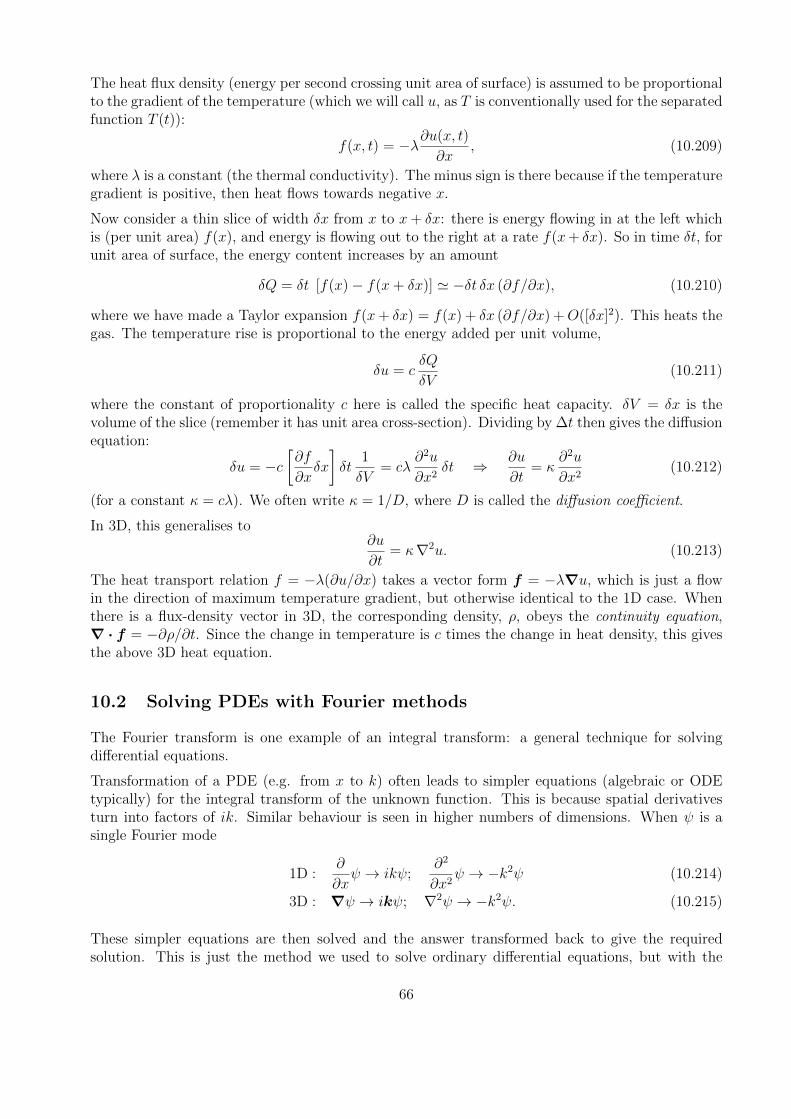
u(x, y, t) = T0

(

1� 16

⇡2

X

m,n odd

1

mnsin

⇣m⇡x

L

⌘

sin⇣n⇡y

L

⌘

exp

�(m2 + n2)⇡2

L2

t

�

)

. (11.269)

74

0

1

2

3

0

1

2

3

0.0

0.5

1.0

0

1

2

3 0

1

2

3

0.90

0.95

1.00

Figure 11.20: Temperature at an early time t = 0.01, for T0

= 1, = 1 and L = ⇡, and then at alate time t = 1.

75