MTH6151 —Partial Differential EquationsWeek 3

2

0.1 The general linear first order pde with variable coef-ficients

In this section we will discuss how to solve the equation

a(x, y)Ux + b(x, y)Uy = c(x, y)U + d(x, y) (1)

where a, b, c and d are functions of the coordinates (x, y). The method of characteristicsused to analyse the equation with constant coefficients can be extended to consider this typeof equations. The point of departure is the geometric perspective we followed in the previoussection.

0.1.1 Geometric approach

Equation (1) can be written as(a(x, y), b(x, y)

)· ∇U = c(x, y)U + d(x, y)

so that∇~vU = c(x, y)U + d(x, y), with ~v ≡

(a(x, y), b(x, y)

).

In this case the vector ~v is no longer constant. This means that the characteristics are nolonger lines but curves. If the characteristics are of the form y = y(x) then they satisfy theordinary differential equation

dy

dx=b(x, y(x))

a(x, y(x)). (2)

Question. Can an ode always be solved?

There is a general result known as Piccard’s theorem that basically says that an odehas always a solution for given initial conditions. Of course, this result does not say (atleast directly) how to solve the equation.

In what follows we assume that we can solve the ode (2). This gives the solution in theform y = y(x). Now, we compute the derivative of U along the characteristics —for this weuse the chain rule as follows:

d

dxU(x, y(x)) =

dx

dx

∂U

∂x+dy

dx

∂U

∂y

= Ux +b(x, y(x))

a(x, y(x))Uy.

Finally, using equation (1) one obtains

d

dxU(x, y(x)) =

c(x, y(x))

a(x, y(x))U +

d(x, y(x))

a(x, y(x)).

This equation is, again, another ode. Its solutions yields the value of U(x, y) along a givencharacteristic curve.

0.1. THE GENERAL LINEAR FIRST ORDER PDE WITH VARIABLE COEFFICIENTS 3

Note. If the characteristic curves cover the whole plane R2, then one obtains a solutionto equation (1) on the whole of R2. On the other hand, if the characteristics do notexist somewhere, then the solution breaks down there —intuitively, one can say that thesolution does not know where to go!

0.1.2 Examples

We now exemplify the general theory of the previous subsection with a number of examples.

Example 0.1.1. Find the general solution of

Ux + yUy = 0.

The equation an be rewritten as(1, y) · ∇U = 0,

so that U is constant along the curves with tangent given by ~v = (1, y). The slope of thecurves is y/1 and, hence, the ordinary differential equation to be solved is

dy

dx= y.

The solutions are given

y(x) = Cex, with C a constant.

These are the characteristics of the pde. A plot for various values of C is given below.

0.5 1.0 1.5 2.0

!15

!10

!5

5

10

15

It is observed that, in fact, the whole planes can be covered by these curves by varying C—i.e.

R2 = {(x, y) | y = Cex, C ∈ R}.Now, observe that for U(x, y(x)) = U(x,Cex) one has that

d

dxU(x,Cex) = Ux + CexUy

= Ux + yUy = 0.

4

Thus, along each characteristic curve the solution is a constant and the solution can onlydepend on C —that is,

U(x, y) = f(C).

In order to obtain the value of the constant it is sufficient to evaluate at a single point foreach curve. For this solution a good point is x = 0. Thus,

U(x,Cex) = constant

= U(0, Ce0) = U(0, C).

However, as y = Cex, one has that C = ye−xso that

U(x, y) = U(0, C) = U(0, ye−x).

In other words, the solution depends only on the combination ye−x. Hence, one can write thegeneral solution as

U(x, y) = f(ye−x),

where f is an arbitrary function of a single variable.

Example 0.1.2. Find the solution to the boundary value problem

Ux + yUy = 0,

U(0, y) = y3.

From the previous example we know that the general solution is given by

U(x, y) = f(ye−x)

so that using that if x = 0 then y = Ce0 = C so that

U(0, y) = f(y) = f(C)

But one also has thatU(0, y) = y3 = C3

Hence, f(C) = C3 and the required solution is given by

U(x, y) =(ye−x

)3= y3e−3x.

Exercise. Check by direct computation that U(x, y) = y3e−3x is, indeed, the required solution.

Example 0.1.3. Find the general solution to

(1 + x2)Ux + Uy = 0.

In this case the equation for the characteristic curves is given by

dy

dx=

1

1 + x2.

The solution to this ode is given by (why?):

y(x) = arctan x+ C, C a constant.

A plot of the characteristics for various values of C is given below.

0.1. THE GENERAL LINEAR FIRST ORDER PDE WITH VARIABLE COEFFICIENTS 5

!4 !2 2 4

!3

!2

!1

1

2

3

Again one can check that they actually cover the whole plane.Now, from the general theory one has that

U(x, arctanx+ C)

is constant along the characteristics —of course, one can also verify it by direct computation.Hence,

U(x, arctanx+ C) = f(C) = constant for given C.

On the other hand one has that

C = y − arctanx

so that

U(x, y) = U(0, y − arctanx) = f(y − arctanx),

with f a function of a single argument. This is the general solution of the equation.

Example 0.1.4. Find the general solution to

Ux + 2xy2Uy = 0.

In this case the equation for the characteristics is given by

dy

dx= 2xy2.

It follows that ∫dy

y2=

∫2xdx+ C.

Integrating one gets

−1

y= x2 + C,

so that after some reorganisation one ends up with

y =1

C − x2.

A plot of the characteristic curves for various choices of C are given below.

6

!4 !2 2 4

!2

!1

1

2

Note that the curves do not seem to fill the plane so that the solution may not exists for all(x, y). Again, from general theory we know that U(x, y) is constant along these curves. Thatis,

U(x, y(x)) = f(C).

Observing that in this case

C = x2 +1

y

one concludes that the required general solution is given by

U(x, y) = f

(x2 +

1

y

).

Example 0.1.5. Find the solution to the boundary value problem√1− x2Ux + Uy = 0,

U(0, y) = y.

In this case the ode for the characteristic curves is given by

dy

dx=

1√1− x2

.

The general solution to this ode is

y(x) = arcsin x+ C

—why? A plot of the curves for various values of C is given below:

!2 !1 1 2

!3

!2

!1

1

2

3

0.1. THE GENERAL LINEAR FIRST ORDER PDE WITH VARIABLE COEFFICIENTS 7

Observe, again, that the curves do not cover the whole plane. Now, by the general theory (ordirect computation)

d

dxU(x, y(x)) = 0,

so thatU(x, y(x)) = f(C).

Hence, the general solution to the equation is given by

U(x, y) = f(y − arcsinx).

Evaluating at x = 0 one finds that U(0, y) = f(y). Thus, comparing with the boundarycondition one concludes that f(y) = y. Hence, the solution we look for is

U(x, y) = y − arcsinx.

Example 0.1.6. Find the general solution to the equation

Ut + xUx = sin t.

This is an example of an inhomogeneous equation. The ode for the characteristics is in thiscase given by

dt

dx=

1

x.

The general solution to this equation is given by

t(x) = ln x+ C.

It will be convenient to rewrite the latter in a slightly different form: t = lnx+ lnC, so thatt = lnCx. A plot of the curves for various values of C is given below:

0.5 1.0 1.5 2.0

!6

!4

!2

2

From the general theory (or direct computation) one further obtains the ode

d

dtU(x, t(x)) =

sin t

x

Expressing t in terms of x using the equation for the characteristic curves one finally finds that

dU

dx=

sin ln(Cx)

x.

8

Using a the substitution z = lnCx one has that∫sin ln(Cx)

xdx =

∫sin zdz = −cosz = − cos lnCx,

so thatU = − cos lnCx+ f(C).

Eliminating C using C = et/x one concludes that

U(x, t) = − cos t+ f

(et

x

).

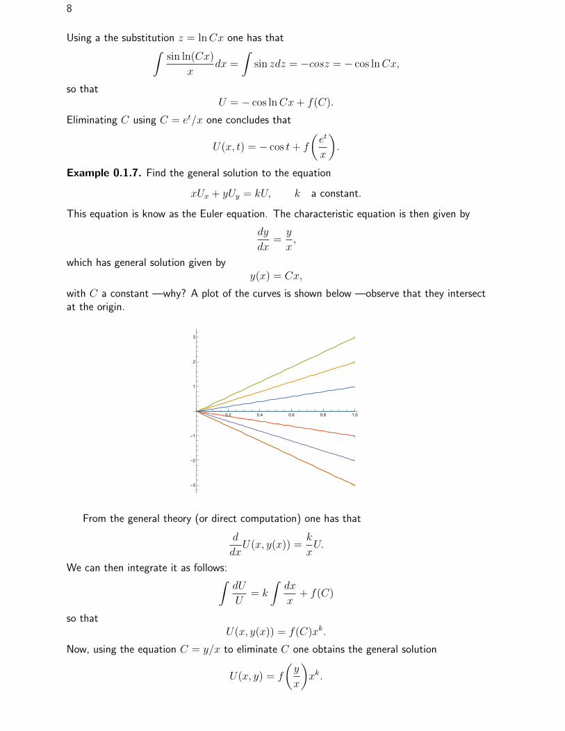
Example 0.1.7. Find the general solution to the equation

xUx + yUy = kU, k a constant.

This equation is know as the Euler equation. The characteristic equation is then given by

dy

dx=y

x,

which has general solution given byy(x) = Cx,

with C a constant —why? A plot of the curves is shown below —observe that they intersectat the origin.

0.2 0.4 0.6 0.8 1.0

!3

!2

!1

1

2

3

From the general theory (or direct computation) one has that

d

dxU(x, y(x)) =

k

xU.

We can then integrate it as follows:∫dU

U= k

∫dx

x+ f(C)

so thatU(x, y(x)) = f(C)xk.

Now, using the equation C = y/x to eliminate C one obtains the general solution

U(x, y) = f

(y

x

)xk.

0.1. THE GENERAL LINEAR FIRST ORDER PDE WITH VARIABLE COEFFICIENTS 9

0.1.3 A second application: population models

First order pdes arise in the study of the age distribution in a population.

Populations (of persons, animals, plants...) obey a sort of continuity equation as in thecase of traffic models. The key difference is that members in a population are born and die.So, the number of individuals in a population does not remain constant in time. Let N(x, t)denote the number of individuals of age x at time t. We are interested in knowing whathappens some time later, say at time t+ h. Then

N(x+ h, t+ h) : Number of people of age x+ h at time t+ h,

so that

N(x+h, t+h)−N(x, t) : −(Number of deceases of age in the interval [x, x+ h] in the period [t, t+ h]).

At a given moment of time t the number of deceases of people of age x is proportional tothe number of people at that particular age (roughly). We write this as µ(x, t)N(x, t), whereµ(x, t) > 0 is the mortality rate. The mortality rate depends on the age group and on time—e.g. there is more mortality in early age, and also more in Winter than in Summer. Toobtain the total number of deceases of age in the interval [x, x + h] in the period [t, t + h]one needs to integrate: ∫ h

0

µ(x+ s, t+ s)N(x+ s, t+ s)ds.

Hence, we obtain that

N(x+ h, t+ h)−N(x, t) = −∫ h

0

µ(x+ s, t+ s)N(x+ s, t+ s)ds.

Now, divide by h to obtain

N(x+ h, t+ h)−N(x, t)

h= −1

h

∫ h

0

µ(x+ s, t+ s)N(x+ s, t+ s)ds.

Taking the limit as h→ 0 one has that

limh→0

N(x+ h, t+ h)−N(x, t)

h=dN

dh|h=0,

and that

limh→0

=1

h

∫ h

0

µ(x+ s, t+ s)N(x+ s, t+ s)ds = µ(x, t)N(x, t),

where in the last equality on has used L’Hopital’s rule to evaluate the limit. Finally, using thechain rule we find that

dN

dh=∂(x+ h)

∂h

∂N

∂(x+ h)+∂(t+ h)

∂h

∂N

∂(t+ h),

so thatdN

dh

∣∣∣∣h=0

=∂N

∂x+∂N

∂t.

Then in a simple model (ignoring, say immigration and emigration) one has that

Nx +Nt = −µ(x, t)N(x, t).

In principle, one knowsN(x, 0) = f(x)

—that is, the initial distribution of population. Some examples are given below:

10

0.1. THE GENERAL LINEAR FIRST ORDER PDE WITH VARIABLE COEFFICIENTS 11

The function f(x) is roughly obtaining by adding the male/female figures together. Onealso requires boundary data N(0, t) = g(t) which corresponds to the number of births at timet.

On this models one can readily see that the characteristics are of the form

t = x+ C,

that is, they are lines. A plot illustrating what happens is shown below:

t

x

N(0,t)=g(t)

N(x,0)=f(x)

I

II

characteristichittingboundarydata

characteristic hittinginitial data

Observe that region I receives only information about the boundary, while II recieves in-formation about the initial condition. Also, one can see that if g(t) = 0 (no births), thepopulation eventually dies.

Remark 0.1.8. There is a complication in the model: in a realistic population model, thenumber of births depends on N(x, t) —that is, the boundary data! A good model describingthis is

N(0, t) ≡ g(t) =

∫ ∞0

λ(x, t)N(x, t)dx,

where λ(x, t) is the so-called fecundity rate. This complicates the model considerably and wewill not dwell into it further.

12

Progress Check1. What is a characteristic curve?

Chapter 1

Second order pde’s with constantcoefficients

In this section we briefly look at the classification of second order partial differential equationswith constant coefficients.

1.1 Introduction

The most general second order partial differential equation with constant coefficients is givenby

aUxx + 2bUxy + cUyy + dUx + eUy + fU = h(x, y) (1.1)

witha, b, c, d, e, f,

are constants and h(x, y) is an arbitrary function. The terms with the highest order derivatives,namely

aUxx + 2bUxy + cUyy (1.2)

are called the principal part. It determines the character of the solutions of the equation. Inthe following, to avoid messy computations, we consider only the principal part —i.e. we setd, e and f to zero. Particular cases of equation (1.1) are

Uxx − Utt = 0 (wave equation),

Uxx + Uyy = 0 (Laplace equation),

Uxx − Ut = 0 (heat equation).

The solutions to each of these equations have a completely different behaviour. In the follow-ing, we will see that, in a sense, these are the only possibilities.

1.2 Quadratic forms

The basic observation is the following: compare the principal part (1.2) with the quadraticform

ax2 + 2bxy + cy2.

We know from basic geometry that the solutions to the equation defined by this quadraticform represents a conic section —i.e. a hyperbola, a parabola or an ellipse. The type of conic

13

14 CHAPTER 1. SECOND ORDER PDE’S WITH CONSTANT COEFFICIENTS

section depends on the coefficients in the quadratic form. More precisely, completing squaresone has that

ax2 + 2bxy + cy2 = a

((x+

b

ay

)2

+

(ac− b2

a2

)y2

).

One then has the following classification:

b2 − ac > 0 hyperbola,

b2 − ac = 0 parabola,

b2 − ac < 0 ellipse.

One can do something similar with the principal part (1.2). One can readily check that

aUxx + 2bUxy + cUyy = a

((∂

∂x+b

a

∂

∂y

)2

+

(ac− b2

a2

)∂

∂y2

)U.

Accordingly, one classifies the pde’s according to the same criteria as for the quadratic forms—more precisely, one says that (1.1) is

b2 − ac > 0 hyperbolic pde,

b2 − ac = 0 parabolic pde,

b2 − ac < 0 ellipse pde.

One can readily check that

wave equation hyperbolic,

Laplace equation elliptic,

heat equation parabolic.

1.3 A change of variables

Consider now new coordiates (x′, y′) given by

x′ = x,

y′ = − bax+ y,

so that

x = x′,

y = y′ +b

ax.

Using the chain rule for partial derivatives one finds that

∂

∂y′=

∂

∂y,

∂

∂x′=

∂

∂x+b

a

∂

∂y.

1.3. A CHANGE OF VARIABLES 15

Substituting the above into the principal part (1.2) a calculation readily gives

aUxx + 2bUxy + cUyy = a

(Ux′x′ +

(ac− b2

a2

)Uy′y′

).

Now, if ac− b2 < 0 one can write

Ux′x′ +

(ac− b2

a2

)Uy′y′ = Ux′x′ − |ac− b

2||a|2

Uy′y′

=

(∂

∂x′+

√|ac− b2||a|

∂

∂y′

)(∂

∂x′−√|ac− b2||a|

∂

∂y′

)U.

In fact, one can eliminate the factor√|ac− b2|/|a| by a further change of variables.

Note. The classification also works if the coefficients depend on the coordinates. In that casethe character of the equation can change from point to point. As an example one has theequation

Uxx + xUyy = 0.

16 CHAPTER 1. SECOND ORDER PDE’S WITH CONSTANT COEFFICIENTS

Progress Check1. What is a characteristic curve? How do you determine then for a linear first order

equation?

2. What is the ode satisfied by the solution toa first order pde along a characteristiccurve?

3. What happens when the characteristic curves do not cover the whole plane?

4. What happens when two (or more) characteristic curves intersect?

5. How do you classify second order pde’s with constant coefficients?

6. What is the advantage of using an appropriate change of coordinates when solvinga second order pde?