simultaneous levitation & power by induction
TRANSCRIPT
S W A R T H M O R E C O L L E G E D E P A R T M E N T O F E N G I N E E R I N G
SIMULTANEOUS LEVITATION & POWER
BY INDUCTION RICHARD METZLER ’06
S E N I O R D E S I G N T H E S I S : F I N A L R E P O R TA D V I S O R : E R I K C H E E V E R
S U B M I T T E D M A Y 4 , 2 0 0 6

2
E 9 0 : F I N A L R E P O RT SIMULTANEOUS LEVITATION & POWER BY INDUCTION
TABLE OF CONTENTS
ABSTRACT………………………………………………………………………...………3
INTRODUCTION…………………………………………………………………………4 DESIGN…………………………………………………………………………………....6
SOLENOID DESIGN……………………………………………………………………6 INITIAL CRITERIA…………………………………………………………………....6 MATERIALS SELECTION…………………………………………………………….11 CONSTRUCTION & MODIFICATION…………………………………………………15 POWER SUPPLY REVISITED…………………………………………………………19
POSITION SENSING……………………………………………………………………21 THEORY…………………………………………………………………………….21 CIRCUIT…………………………………………………………………………….24
CONTROL……………………………………………………………………………….26 SYSTEM CHARACTERIZATION……………………………………………………….26 COMPENSATOR DESIGN……………………………………………………………..30 IMPLEMENTATION…………………………………………………………………..33
DISCUSSION & CONCLUDING REMARKS……………………………………………35
ACKNOWLEDGEMENTS………………………………………………………………..36 REFERENCES…………………………………………………………………………...36 APPENDIX………………………………………………………………………………38
2

3
Figure 1: Levitation System
ABSTRACT
The goal of this project is to simultaneously levitate and power an autonomous device in a controlled manner. The system of particular interest—a conductive ring, driven by a solenoid—could be used to power machinery mounted on the ring without the means of an onboard power supply. This induced power is supplied by the stored momentum of the magnetic field generated by the solenoid when the field is altered. The induced current in the ring is be rectified and used to run electrical components on the ring itself, without the added weight of a battery. Thus, the design of this control unit could lead to the eventual design of a circuit that can run automatically from induced power, and could be controlled to move in three dimensions by adjustment of feedback controlled electromagnets.
3
4
INTRODUCTION
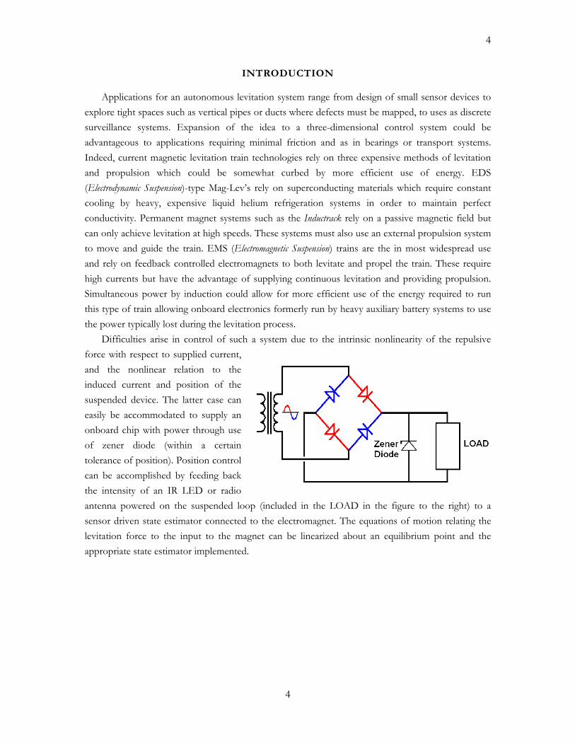
Applications for an autonomous levitation system range from design of small sensor devices to explore tight spaces such as vertical pipes or ducts where defects must be mapped, to uses as discrete surveillance systems. Expansion of the idea to a three-dimensional control system could be advantageous to applications requiring minimal friction and as in bearings or transport systems. Indeed, current magnetic levitation train technologies rely on three expensive methods of levitation and propulsion which could be somewhat curbed by more efficient use of energy. EDS (Electrodynamic Suspension)-type Mag-Lev’s rely on superconducting materials which require constant cooling by heavy, expensive liquid helium refrigeration systems in order to maintain perfect conductivity. Permanent magnet systems such as the Inductrack rely on a passive magnetic field but can only achieve levitation at high speeds. These systems must also use an external propulsion system to move and guide the train. EMS (Electromagnetic Suspension) trains are the in most widespread use and rely on feedback controlled electromagnets to both levitate and propel the train. These require high currents but have the advantage of supplying continuous levitation and providing propulsion. Simultaneous power by induction could allow for more efficient use of the energy required to run this type of train allowing onboard electronics formerly run by heavy auxiliary battery systems to use the power typically lost during the levitation process. Difficulties arise in control of such a system due to the intrinsic nonlinearity of the repulsive force with respect to supplied current, and the nonlinear relation to the induced current and position of the suspended device. The latter case can easily be accommodated to supply an onboard chip with power through use of zener diode (within a certain tolerance of position). Position control can be accomplished by feeding back the intensity of an IR LED or radio antenna powered on the suspended loop (included in the LOAD in the figure to the right) to a sensor driven state estimator connected to the electromagnet. The equations of motion relating the levitation force to the input to the magnet can be linearized about an equilibrium point and the appropriate state estimator implemented.
4

5
Figure 2: Photoelectric Position Feedback System in Proposed Levitation Device.
5

6
DESIGN
I. SOLENOID DESIGN: INITIAL CRITERIA
Originally, a conductive coil was to be levitated above the power solenoid by the Lorentz force law. This repulsive force is proportional to the time derivative of the supplied magnetic field from the power solenoid. Thus, if the solenoid is powered by a sinusoidal voltage, the force is proportional to the amplitude A times the natural frequency ω. A simple model for the power solenoid is given by the RLC circuit shown below
V
36 V 10MHz 0Deg
C1nF
L860mH
R
14 Ω 1
2
3
4 Figure 3: 2nd Order Solenoid Model
with the generated field proportional to the current. To maximize the repulsive force without requiring significant power consumption, the solenoid would be wound such that its resonant frequency would be about 10 MHz.
Figure 4: The system. A current i t is driven through the solenoid. This current will produce a force on the
ring that is proportional to the current and to the height( ) zF
Z of the ring itself.
6

7
We begin by defining the force on the ring by using the Lorentz Force Law, which states that the
repulsive force on a unit with a current I due to a magnetic field B is given by:
( )F I dl B= ×∫ (1)
The total force on the ring will then be the integral of the Lorentz law (1), applied to some differential length in the ring. We know from symmetry that the net force must be in the
direction: all other components will cancel out when we take the integral around the loop. From (1) above we get:
dlz
ˆzF dl I Bθ r= ⋅ ⋅∫ (2)
where we have taken the scalar components of the vector quantities B and ˆIθ
as we are only
interested in one component of each (we set rB B= and ˆI Iθ
= ). We find that the current and
the magnetic component are symmetric around the loop, so the integral is becomes trivial, and we get:
2z ringF r I rBπ= ⋅ ⋅ (3)
Now, we can use the geometry of the system to find rB . We take as a control volume a
cylinder the size of the ring, with radius , and some differential height : r dz
Figure 5: The flux diagram for the cylindrical control volume. We see that the total flux must be equal to zero, so the flux
lost through the sides must be the net flux gained through the top and bottom.
We must have a total flux equal to zero in our control volume, since it only contains empty space. We know we gain some flux through the bottom, lose some through the top, and also lose
7

8
some through the sides. We have expressed these values above as a product of the magnetic flux density and the surface area. By setting the total flux equal to zero to satisfy this continuity condition, we get:
20 2 rBrB rz
π π ∂= −
∂ (4.a)
which simplifies to:
2z
rdBrBdz
−= (4.b)
Then,
2 2 ringz ring
ring
VdB dBF r I rdz dz R
π π= − ⋅ ⋅ = − ⋅ ⋅ (5)
where
( )2
3/ 22 2( , )
2oNi RB z i
R z
µ=
+ (6)
and is the induced EMF in the ring, which is given by Faraday’s Law:ringV 1
( )
MF
22
0 3/ 22 2
( )
( )
z
sol sol
sol
dBdV Adt dt
R di tr NdtR Z t
π µ
ΕΦ
= − = − ⋅
= − ⋅+
(6.a)
Here N is the number density of windings in the solenoid, and we have assume that Z(t) does not change appreciably in time. Thus, the simple result for the induced voltage is
1 Griffiths
8
9
( )MF 3/ 22 2
( )
( )sol
sol
di tKVdtR Z t
θΕ
−= − ⋅
+ (6.b)
where is a constant lumping up the messy system parameters and theta is some phase lag owing to the self inductance of the ring (we will return to this later).
K
We also need an expression for zdBdz
, for which we get2:
( ) ( )
20
3/ 2 5/ 22 2 2 2
( ) ( ) ( )2 ( ) ( )
sol sol solz
sol sol
i t N R C Z t i tdBdz z R Z t R Z t
µ⎡ ⎤ ⋅ ⋅∂ ⎢ ⎥= = −⎢ ⎥∂ + +⎣ ⎦
(7) where we have again grouped constants into C for brevity. Plugging (6) and (7) back into (5), we get:
( ) ( )
( )
3/ 2 5/ 22 2 2 2
2 2
2 ( ) ( ) ( )( )
( ) ( ) ( )( )
( ) ( )( )
z sring sol sol
sol sol
sol
sol sol
K C Z tF iR R Z R Z t
Z t i t i tDR Z t
D i t i tZ t
ol solt i tπ θ
θ
θ
−
⋅ ′= ⋅+ +
′⋅ ⋅ −=
+
′⋅ ⋅ −≈
−
(8)
where we have assumed in the last approximation that the distance Z(t) above the solenoid is much larger than the radius of the solenoid itself.
We can now find the equations of motion by using Newton’s First Law ( ). We
assume that the only forces acting on the system are gravity and the Lorentz Force, so we wind up getting:
( )F mZ t=
( ) ( )D i t i tmZ mg
Zθ′⋅ ⋅ −
= −
(9.a)
Or
2 Griffiths
9

10
( ) ( )D i t i tz
m Zgθ′⋅ −
= − (9.b)
The derivative term can be misleading in that the force is not generated by the current of the solenoid; rather, it is generated by the opposing magnetic fields of the ring and the solenoid (which has an i(t) dependence) and the ring (which is dependent on the derivative of i(t)). The phase lag θ is included here to indicate that the opposing magnetic field of the ring is not necessarily instantaneously induced by the oscillating magnetic field of the solenoid. In fact the
ring itself is an inductor and will introduce this phase lag between the generated current and the induced EMF generated by the solenoid current. If the capacitance of the between the coils is negligible, we can use a simple RL circuit to model this. Notice that the average force is zero unless the field generating current, isol, is in phase with the induced current’s derivative.3 We can use the self-impedance relationship for the ring to find the phase lag of induced current’s derivative in terms of the EMF voltage generated by isol:4
( ) ( ) ( ) ( )( EMF1
sol ring ringi t i t V t R i tL
θ′ ′− = = − ⋅ ) (10)
where R is the resistance of the ring and is its self-inductance. Taking the Laplace Transform and solving for the transfer function of the derivative we get:
L
1( )1
sT sLR sR
= ⋅⎛ ⎞+⎜ ⎟⎝ ⎠
(11)
We get the following Bode plot:
3 Notice that for any periodic waveform such as a sinusoid, the derivative is 90° out of phase. Thus the average of the signal times its derivative must be an odd function with average zero. 4 Purcell
10
11
0
10
20
30
40
50
60
Mag
nitu
de (d
B)
106
107
108
109
1010
0
30
60
90
Phas
e (d
eg)
Bode Diagram
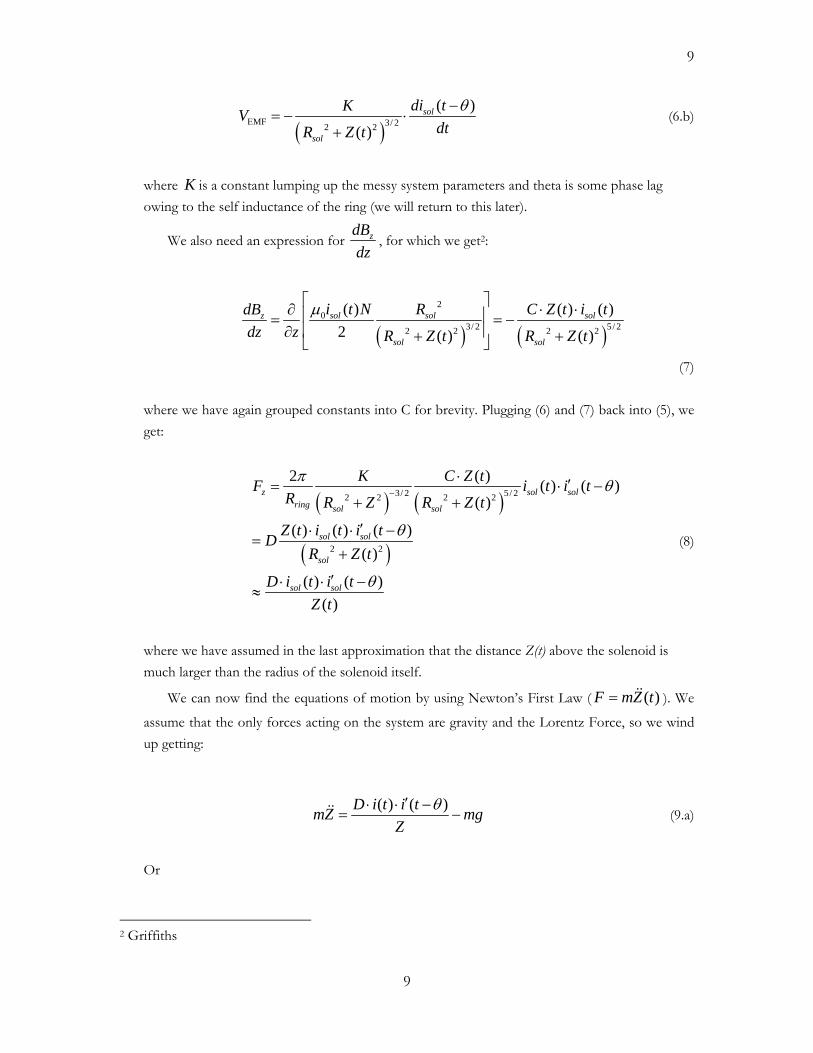
Frequency (rad/sec) Figure 6: Bode Plot of Current through Levitation Ring
where we can see that the phase only approaches zero when the circuit is driven an order of magnitude greater than the pole frequency L/R where it also approaches its maximum gain. Thus, experimentally it appears that the induced force is proportional to the square of the amplitude of the supplied solenoid current over the height of flotation for high driving frequencies with respect to L/R.:
2 ( )i tz k gmZ
≈ − (9.c)
MATERIALS SELECTION
In constructing the power solenoid, special care was taken to use the proper materials to produce the maximum field strength that could be oscillated megahertz frequencies. Here I will discuss some of the concepts involved in materials selection of suitable magnetic materials.
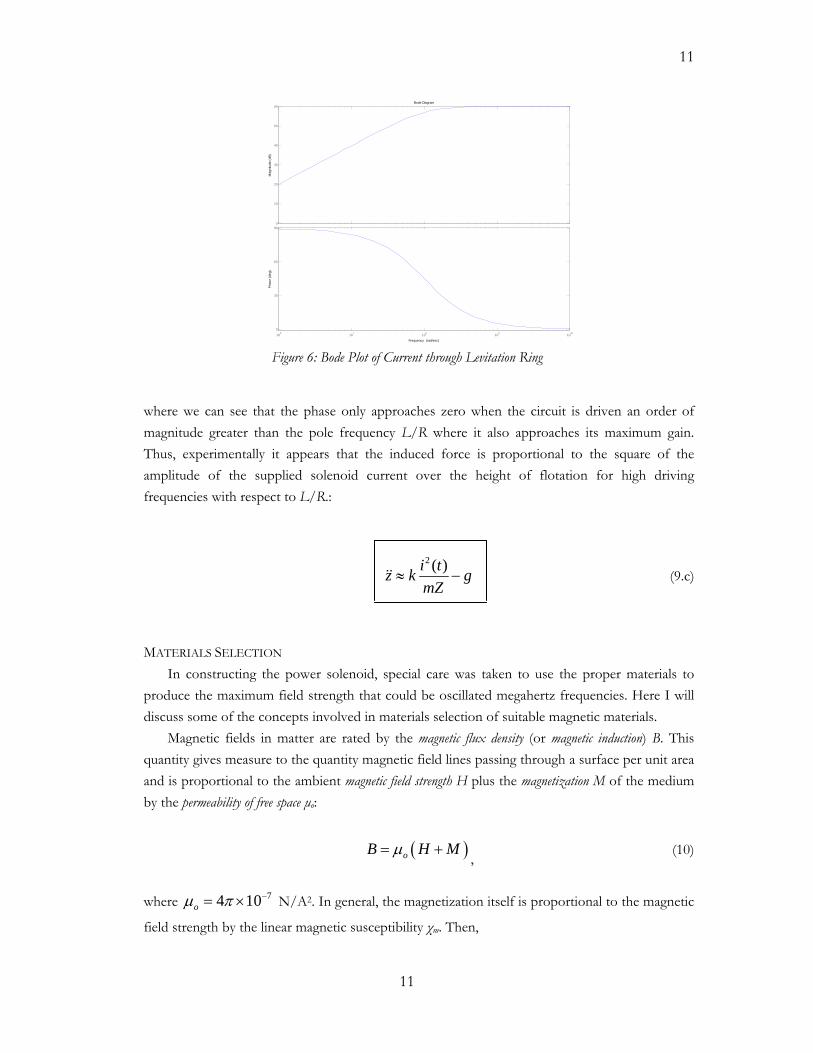
Magnetic fields in matter are rated by the magnetic flux density (or magnetic induction) B. This quantity gives measure to the quantity magnetic field lines passing through a surface per unit area and is proportional to the ambient magnetic field strength H plus the magnetization M of the medium by the permeability of free space µo:
( )oB H Mµ= + , (10)
where N/A74 10oµ π −= × 2. In general, the magnetization itself is proportional to the magnetic
field strength by the linear magnetic susceptibility χm. Then,
11

12
( )1
o mB HH
µ χµ
= +
= (11)
where µ is the medium’s magnetic permeability. Often however, materials are characterized by their relative permeability
ro
µµµ
= . (12)
In order to support and enhance the magnetic field strength H supplied by a current-carrying
coil, high permeability ferromagnetic materials should be used for a solenoid’s core.
5
Figure 7: Magnetic Fields trough Vacuum and through Iron
One must also consider that the saturation flux density of any given material will limit its maximal performance; that is, once the magnitude of the field strength reaches a certain value, all magnetic dipoles will be aligned with the field and further magnetization cannot take place. Typically, iron has a saturation flux density of about 2 T. This is an upper value in typical NMR machines. In cores which must support magnetic fields greater than this such as in an MRI which requires flux densities of 40 T, air can be used as the core material as it will not saturate. However, because air has a relative permeability of only 1, one would need to provide 150 times more field strength than necessary to generate the same flux density within an iron core with a typical relative permeability of 150.
Another important factor is hysteresis loss. The graph below shows the B field as a function of the H field.
5 http://hyperphysics.phy-astr.gsu.edu/hbase/magnetic/elemag.html#c4
12

13
Figure 7
Figure 8: B vs H of a typical ferromagnetic material.
Note that the magnetic flux density is path dependent. In traversing the curve, the area enclosed by the path is the energy cost of changing the magnetization of a material. This is usually released as thermal energy at the expense of the induced field in a solenoid core. The saturation flux density can also be determined from the curve and is given by magnitude at the cusps of the hysteresis curve where the magnitude of B approaches the horizontal asymptote. The permeability of the material is given by the slope of the curve at any given point and is seen to be dependent on H. The initial permeability is that given on most data tables and is the slope of the path starting from the origin. Here is good place to elucidate the meaning of permeability: It is a measure of how easy/difficult it is to rotate the magnetic dipoles within a medium.
Materials that have a narrow hysteresis curve experience little energy loss in the presence of a changing H field and are dubbed “soft” magnetic materials. These usually have steep curves originating from the origin and thus have very high initial permeabilities. “Hard” magnetic materials on the other hand undergo massive core loss and require massive amounts of energy to change their magnetization. For this reason, hard magnetic materials have a large remenancy; that is, they generally hold their magnetization indefinitely unless forcefully altered.
13

14
6
Figure 9: Hysteresis Curves of Hard and Soft Magnetic Materials
For these reasons, soft magnetic materials are preferred for AC operation. A table of soft magnetic materials is given below and a chart of hard magnetic materials in the following section.
Table 1: Table of Soft Magnetic Materials
6 Callister, 690
14

15
Table 2: Soft Magnetic Materials Listing from Ed Fagan Inc.7
Typical DC Magnetic Properties EFI 79 EFI 50 EFI Co50 EFI Core Iron EFI Vac Iron
Saturation Induction - Gauss 8,700 14,500 24,200 21,500 21,500 Maximum Permeability 230,000 100,000 10,000 10,000 10,0000
Coercive Force - Oersteds 0.015 0.060 0.400 1.000 1.000 amps per m 1.19 4.77 31.83 79.58 79.58
Typical AC Magnetic Properties Core Loss W/lb @400Hz & 20k G N/A N/A 34 N/A N/A
B-40 Permeabilty @60Hz 45,000 6,500 N/A N/A N/A NA = Not reported, not a typical application value
One other consideration is important to take into account: resistance. An oscillating
magnetic field induces an electromotive force which causes current to flow in the opposite sense to the current supplied through the coil. This manifests in magnetization opposite the desired direction and effectively increases the impedance of the coil. This mutual inductance is exactly what we want in the floatation coil but is a hindrance to the performance of the solenoid of the solenoid. Because of this we require a core material with very high resistance which will keep eddy currents to a minimum. Other tricks can be employed to lessen eddy currents such as eliminating any circular paths for current to flow or by using laminations to prevent current flow from one sheet to the next.
CONSTRUCTION & MODIFICATION Noting that an alternating magnetic field will also induce a back EMF into the winding itself
thereby impeding the flow of current, effort was taken to minimize the self-inductance
2
onLl
µ∝ (13)
The strength of the field depends on n so it is not desirable to minimize this quantity too much, rather, by maximizing the length of the solenoid l we can minimize the self-inductance affordably.
A 7” long, 4” inner diameter steel spool was to be constructed for winding the coil. To maximize the saturation density, EFI Co50 alloy rods were held in a primarily air core by insulative phenolic sleeves which were pressed into the spool which was to be wound with the proper magnet wire.
7 www.edfagan.com
15

16
The proper solenoid winding gauge was determined by an appropriate java script (see APPENDIX) by comparing the winding density (a positive factor in contribution to the net magnetic field) to the net impedance of the solenoid for each gauge. Also considering price constraints and availability, 30 lbs (almost one mile) of AWG 16 gauge magnetic wire rated at 300° C was chosen. The core was wound from 4.3” to 6.9” in diameter (about 21 layers of winding) and had a DC impedance of about 14 Ohms. Winding was done originally to be done on a lathe, but even on the lowest speed setting, windings would jump and slide creating air gaps which decrease the winding density. This was also intolerable because thermal expansion and strain working of the wires during AC operation would cause windings to rub insulation off and short together whole layers. For these reasons, winding of the solenoid was done painstakingly by hand.
In order to reduce the total impedance of the core, it was initially planned to wire every two layers of wiring in parallel with the next two successive layers.
L182mH
L282mH
L382mH
L482mH
L582mH
L682mH
L782mH
L882mH
L982mH
L1082mH
L1182mH
V1
120 V 60 Hz 0Deg
2
1
Z = 8.2 Ohms
V2
120 V 60 Hz 0Deg
L12820mH
3
4 Z = 820 Ohms Figure 10: Dividing Inductance for Solenoid Winding
This reduces the necessary driving voltage to below the safe limit of 48 V but requires a significant amount of amperage. Because the power supplies available for use could only deliver a total of 5.6 A, a continuously wound magnet was built instead, with a maximum possible voltage drop of 70 V to accommodate the limitation. Because a series aligned inductances add while a parallel alignment diminish, the total impedance was sacrificed for current performance, which is the contributor to the magnetic field. However, the power supplies were only able to deliver up to 20 kHz AC current without significant attenuation, limiting the electromagnet’s response orders of magnitude below the ten megahertz resonant frequency.
Inductive power supplied to the solenoid at 5 A amplitude, 20 kHz frequency was insufficient to jump a 7” ID, 8” OD ring without extending the solenoid core through the center of the ring. Because the levitating device was to be completely free-floating, this was an unacceptable condition.
16

17
To compromise for the lack of repulsive force, the entire system was flipped upside-down and the solenoid was fitted with a 3” diameter, one inch thick, high power N48 neodymium magnet.
Figure 11: Solenoid with Permanent Magnet
At the time, N48 was the highest grade magnet available in size. Several weeks later higher grades N50 and N52 advertising higher flux densities came on the market.
The magnet alone allows astable floatation of a one inch diameter by one inch thick N50 neodymium magnet up to 8 inches. However, because a hard magnetic material is now introduced to the core (already near saturation) further boosting of the auxiliary field produced by the coil is limited.
17
18
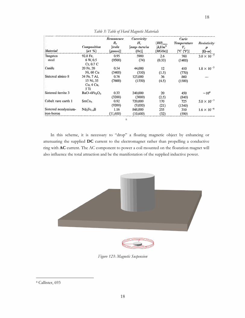
Table 3: Table of Hard Magnetic Materials
8
In this scheme, it is necessary to “drop” a floating magnetic object by enhancing or attenuating the supplied DC current to the electromagnet rather than propelling a conductive ring with AC current. The AC component to power a coil mounted on the floatation magnet will also influence the total attraction and be the manifestation of the supplied inductive power.
Figure 123: Magnetic Suspension
8 Callister, 693
18

19
The force between two magnetic fields is proportional to the net flux between the generators of those fields. In thus case a solenoid, a large permanent magnet, and a floating permanent magnet contribute the total flux. Geometrically, the magnet field of a cylindrical magnet and the magnetic field of a current carrying coil of wire are indistinguishable. Thus, the total force on the floating magnet will be proportional to its static B-field times that of the solenoid plus its B-field time that of the permanent magnet. Considering Equation (6), the force becomes approximately
( ) ( )
319/ 4 9 / 4
2 4
( , ) mm iF z iz m z m
= +− −
(14)
The mi’’s are fit parameters grouping all the geometrical factors found in the similar derivation of the inductive force. m1 and m3 scale the strength of the solenoid and the permanent magnet, respectively, while m2 and m4 account for the effective distances from the solenoid to the floating magnet and from the permanent magnet to the floating magnet (with contributions from their radii).
POWER SUPPLY REVISITED Noting that the induced voltage to the levitation coil is proportional to both the frequency
and magnitude of the current in the solenoid wining,
( ) ( )EMF oV t nf i tµ∝ − , (15)
one option to improve power performance is to exchange driving frequency for amplitude. This may be accomplished by driving the solenoid at 60 Hz (near its DC impedance) with substantial current drawn from the AC outlet. On average, the net DC force on the levitating magnet would be zero; however, this current could be rectified to produce an only positive or negative-sensed current to supply the appropriate magnetic field.
A better idea is to rectify both positive and negative components of a wall outlet’s voltage to supply DC power to a fast push-pull amplifier.
19

20
T1
TS_POWER_VIRTUALWall Outlet
C10.1F-POL
C20.1F-POL
C30.1F-POL
C40.1F-POL
C50.1F-POL
C60.1F-POL
C70.1F-POL
C80.1F-POL
C90.1F-POL
C110.1F-POL
1
2
3
4
5
6
7
8
D1
1B4B42
1
2
4
3
11
12
0
V1
120 V 60 Hz 0Deg
14
15
10
Vcc120V
-Vcc-120V
9
240V Wall Outlet Rectifier with 1/2 V Ripple
Figure 13: Rectifying Power from the Wall Outlet
The positive component is taken and smoothed by five 100,00uF capacitors rated at 25V each to minimize ripple to ½ V (0.42%). The same is done on the negative side of the circuit. The outputs are then connected to the terminals of a two stage push-pull amplifier.
20

21
Q3
NDS8852H
Q1
NDS8852H
U1
0.04 sq.m 0.15 mFloatation Device
4 5
VCC120V
NegativeVCC-120V
U2
CLC505AJP
3
2
4
7
6
8
NegativeVCC
VCC
R2
120kΩ
R1
5.1kΩ
2
1
0
3Vin
2-Stage Push-Pull Follower Amplifier
from Computer
Figure 14: Push-Pull Amplifier
The amplifier follows a -5 to 5V output signal from the computer and is limited in speed by the op-amp (the transistors in use here are relatively fast). The output of the controller can be effectively amplified to up to 240V as the first stage of the amplifier pulls one terminal of the load up to +120V while the second stage pulls the other terminal down to -120 V (and vise-versa).
If faster switching speeds are required for induction, a comparator with a PWM input signal from the computer could be used instead of the op-amp. This would not be difficult to realize implement; however, because of time constraints, converting the output from the controller to a PWM signal was never implemented.
II. POSITION SENSING: THEORY
To complete the feedback loop it is necessary to know something about the state of the levitating object. This can be accomplished by position sensing. There are several methods of doing this:
Hall Effect Sensing One Hall Sensor is placed in a location where it can only measure the B field of the
solenoid.
21
22
Another is placed in a location where it measures the total field from the solenoid and the floatation magnet.
Based on the difference between the signals the position of he floating magnet can be determined.
This method can be unreliable and is subject to interference.
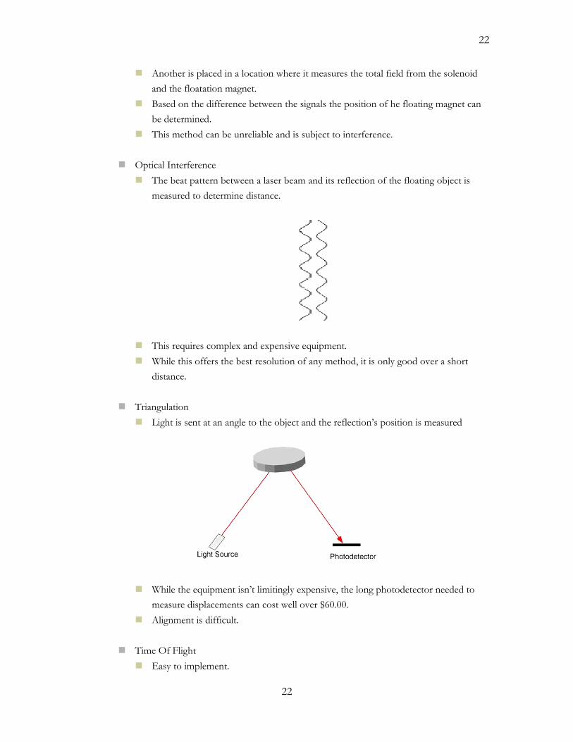
Optical Interference The beat pattern between a laser beam and its reflection of the floating object is
measured to determine distance.
This requires complex and expensive equipment. While this offers the best resolution of any method, it is only good over a short
distance.
Triangulation Light is sent at an angle to the object and the reflection’s position is measured
While the equipment isn’t limitingly expensive, the long photodetector needed to measure displacements can cost well over $60.00.
Alignment is difficult.
Time Of Flight Easy to implement.
22

23
Requires fast electronics for nanosecond measurements.
Optical Intensity
ment. ich limits speed of acquisition.
Although I considered using triangulation, the last two methods appeared to be better at pro
or the time of flight method, laser light is be pulsed and the time it takes to return to a pho
Accurate measurement.
Easy to imple Requires filtering wh Reasonably accurate measurement.
viding distance data over long distances. I will go into more detail on these methods below. Ftodiode receiver will provide two times the distance to the object off which the pulse is
reflected:
2ctd = (16)
Similar measurements can also be achieved using ultrasound.
For a cost effective solution, the magnitude of a certain wavelength of light reflected from th
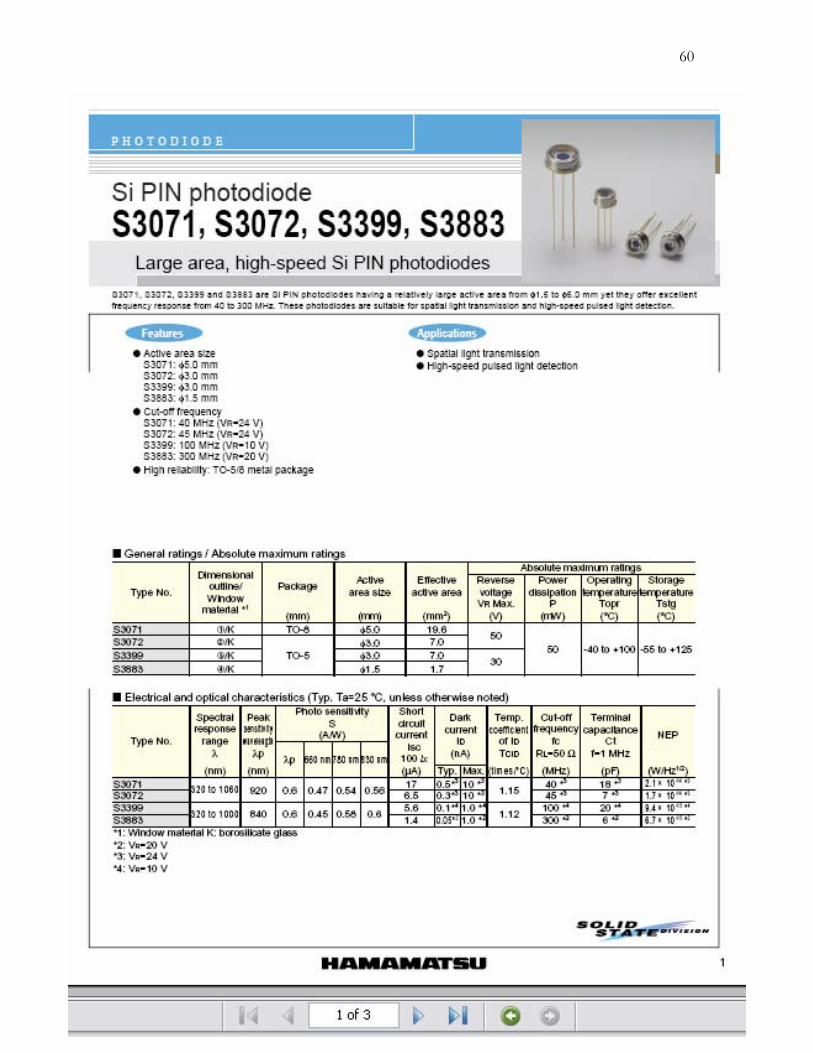
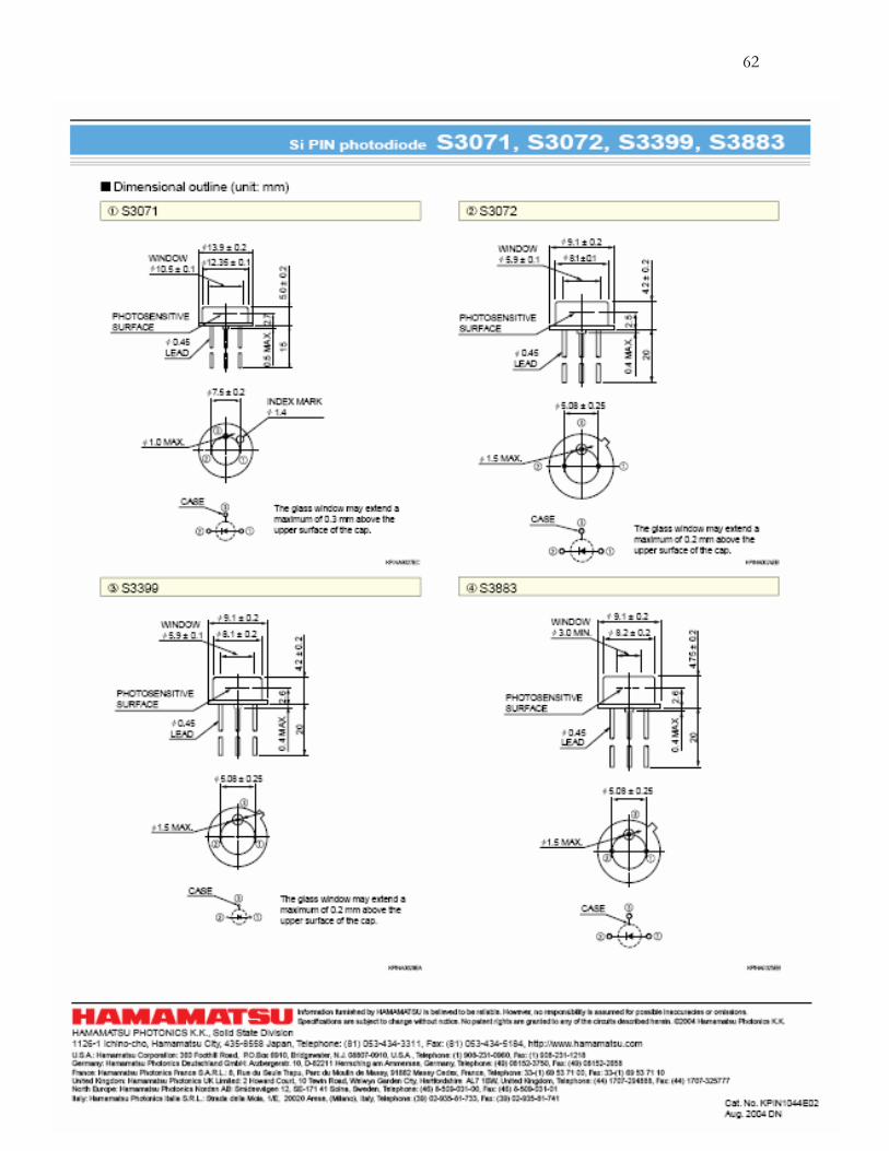
e object of interest can be measured. This is the optical intensity method. In this case, an IR LED is flashed at 20 kHz and is received by a photodiode. The photodiode’s output is digitally filtered to produce only the clocked Fourier spectrum and the magnitude measured to determine the distance regardless of ambient conditions. The output must be calibrated against the known position (leading to inaccuracies) and the method is also relatively slow. For these two reasons, modern control techniques cannot be used as accurate derivative (velocity) feedback cannot be obtained. An example output from the system is shown below:
23

24
Figure 16: Position Detector Signal Output (in Volts)
For better accuracy and speed an IR laser could be used instead of the LEDs. Although IR laser diodes are readily available for about $20, pulsed versions require a relatively large supply current (typically 1.4 to 12A). Without stringing together a row of smaller power supplies to provide the necessary current, it was not possible to attain such a current with the equipment available to us (the large power supplies were already in use on the solenoid). I did experiment with one IR laser diode rated with a lasing threshold of 1.4 A. However, the diode was faulty and would not lase for reasonably supplied amperages (up to 4 A).
CIRCUIT
The circuit below was designed using a 555 chip to pulse three 840 nm IRLEDs at 25 kHz. The output is picked up by a photodiode and amplified then fed into a computer for processing.
24

25
LED1
LED2
LED3
D1
DIODE_VIRTUALLTE-5208 Photodiode
R1
27Ω
R339kΩ
R41.0kΩ
C11.2nF
VCC9V
4
5
6
R5
100kΩ
A1
555_VIRTUALGND
DIS
OUTRST
VCC
THR
CON
TRI
1
2
7
C210nF
U1
741
3
2
4
7
6
51
9
8
0
DisplacementDetector
0
VCC
3
R6
100kΩ
10
11
Figure 17: Position Sensor Circuit
The actual board was modified later on to a 20 kHz, approximate 50% duty cycle pulse train which allowed better response from the photodiode detector.
25

26
CONTROL
I. SYSTEM CHARACTERIZATION:
To pick the optimal magnet for levitation one must consider its geometry. Consider a cylindrical magnet cut into thin lateral slices. Each slice contributes to the net flux of the entire system, but because the falloff of the magnetic field with respect to distance is faster then linear, each slice contributes less and less force between it and the permanent magnet in as it grows in distance from the core.
Figure 158: The Flux of two Permanent Magnets
Thus the added weight of each subsequent slice will grow faster than the total force.
Also notice that as the diameter of a slice levitating cylinder increases, it encompasses more
field lines. Thus the force scales at approximately the same rate as the increase in weight for a magnet of larger surface area. Optimally, the best levitation magnet is as thin as possible with the same diameter (3”) as the core magnet.
Out of several different magnets, a 1.5” diameter by 1/8” thickness ND48 magnet was
chosen as the levitator. A 3x1” N48 magnet similar to that in the core provided 50 times more force (at 72 times the mass). Although this magnet’s equilibrium floating position was about ½” less than that of the thinner magnet, its strength would allow for a larger, heavier induction coil and a greater payload. Another 1x1 N50 displayed a significant increase in strength per mass. It could float 10” at 0 amps and carry ample load. However, the latter two magnets both would
26

27
require high current to achieve stability in regions above the equilibrium position nearer to the solenoid.
To measure the force between the magnets, fishing line was connected between a 239.8g
wooden block and a 4.0g polystyrene block. The wooden block was placed on a scale and the levitation magnet floated beneath the polystyrene block. By reading the change in scale reading from the total component weights, the force between the magnets could be determined.
Figure 169: Force Measurement of System
By varying the current from -5 to 5V DC at set string lengths, the force contour vs. current
and drop height could be determined.
27

28
0
0.5
1
1.5
2
2.5
3
3.5
6 8 10 12 14 16
Current Slope & Permanent Magnet Offset Versus Distance
Current Slope (N/A)Current Offset (N)
Cur
rent
Slo
pe (N
/A)
Distance (cm)
Figure 20: Falloff of the force due to the permanent magnet force and the slope of the force due to the solenoid. Above are data points taken at 0 A (blue) and at a constant amperage (2.5 A, red)
corresponding to the interaction with the permanent magnet in the core and the behavior of the solenoid separately. The lower fit fits all constant parameters in the function from Equation (). The upper fit forces the decay rate to (z-m3,4)-9/4 as derived. I assume the second fit is more reliable as the second data point is obviously inaccurate and pulls each curve from its mark to the lower fit.
The magnetic force was found to be
( ) ( )9/ 4 9 / 4
327 18.5( , )1.44 2.53
iF z iz z
= ++ − (17)
considering all data. The functional force contour looks as such:
28
29
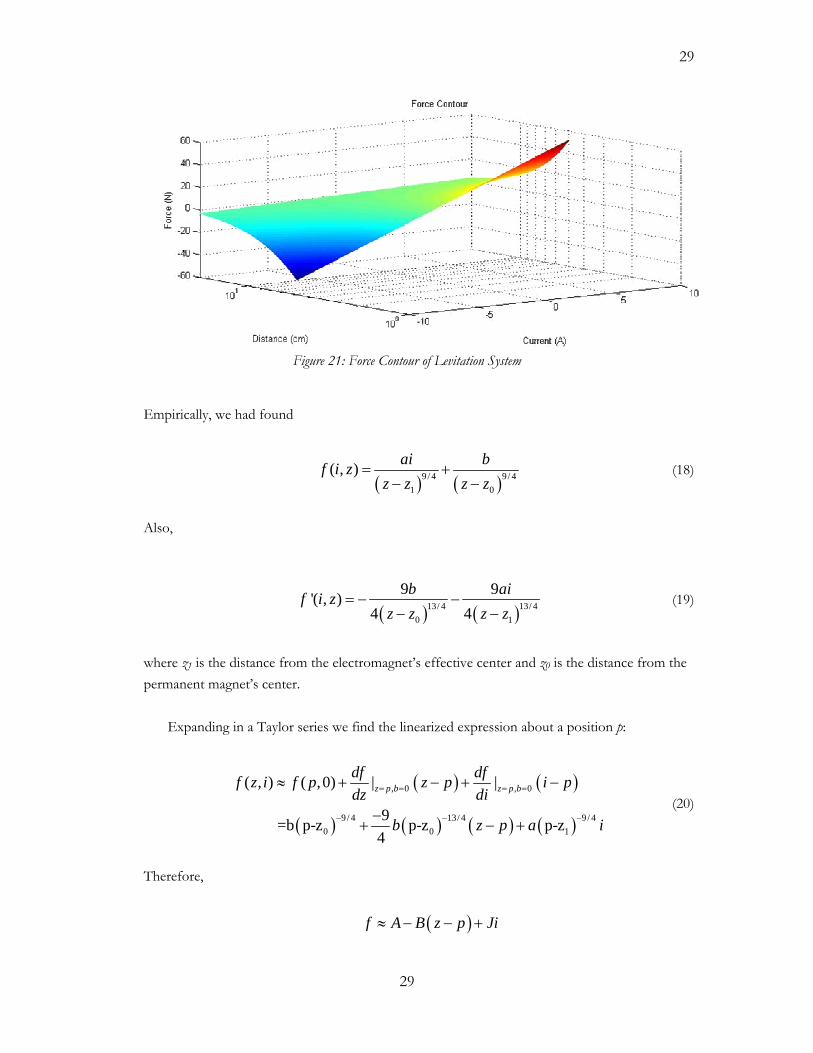
Figure 21: Force Contour of Levitation System
Empirically, we had found
( ) ( )9/ 4 9/ 4
1 0
( , ) ai bf i zz z z z
= +− −
(18)
Also,
( ) ( )13/ 4 13/ 4
0 1
9 9'( , )4 4
b af i zz z z z
= − −− −
i (19)
where z1 is the distance from the electromagnet’s effective center and z0 is the distance from the permanent magnet’s center.
Expanding in a Taylor series we find the linearized expression about a position p:
( ) ( )
( ) ( ) ( ) ( )
, 0 , 0
9 / 4 13/ 4 9 / 40 0
( , ) ( ,0) | |
9 =b p-z p-z p-z4
z p b z p bdf dff z i f p z p i pdz di
b z p a
= = = =
− −
≈ + − + −
−+ − + 1 i−
(20)
Therefore,
( )f A B z p Ji≈ − − +
29

30
where
( )
( )
( )
9/ 4
13/ 4
9 / 4
09 04
1
A b p z
B b p z
J a p z
−
−
−
= −
= −
= −
II. Equations of Motion near Position “p”:
The equation of motion is
mg F mz Dz− = − (21)
where z is the distance from the solenoid base and D is a damping term due to air resistance.
This becomes
z Dz Bz g A Bp Ji+ − = − − − (22)
We’ll substitute in the state variable g Ax z
Bp−
= + − to get rid of the offset on the input
side of the equation. Applying the Laplace Transform, the transfer function is
2( )lJG s
s Ds B= −
+ − (23)
II. COMPENSATOR DESIGN:
The system as a whole can be broken down as such:
30

31
V(s) X(s)p(t)pv
Workspace to Voltage Convertor
20
Power Amplifier
1
Position Sensor
-J
s +D.s-B2
Levitator
Position
FromWorkspace
-s
L.s+R
Electromagnet
0
Display
a1.s+a0
b1.s+1
Controller
Figure 22: Control System Diagram
An input from the MatLab Workspace is converted into a voltage to be output to the system. The gain of the operational amplifier is set at about 20. The signal is sent to the electromagnet, the levitator responds, and the position from the detector is fed back into the controller to compensate the system.
The transfer function of the electromagnet’s current in response to the applied voltage from the controller can be treated as an RLC circuit in series operation. We may also easily adjust the total capacitance by adding an external capacitor in series with the electromagnet to adjust for stability requirements. In this case, we will choose the total capacitance such that its contribution is negligible in order to reduce the order of the model. Assuming we connect the coil to the power supply in reverse sense (to get rid of unwanted negatives in the system transfer function), the electromagnet transfer function becomes
( )msG s
Ls R= −
+ (24)
We will also set the gain of the power amplifier 20 and employ a phase-lead controller to
improve stability. The open loop transfer function is then
( )
( )( )( )1 0
21
20( )
1 *J a s a
G sL b s Ls R s D s B
+=
+ + + − (25)
and the characteristic equation of the open loop transfer function is
( ) ( )
( )
4 31 1 1 1 1 1
1
( ) 20
- - 20 o
C s b Ls b R b DL L s b DR R DL Bb L a J s
DR Bb R BL a J s BR
= + + + + + + − +
+ −
2
(26)
31

32
To satisfy the Routh-Hurwitz stability criterion we can quickly see that b1 must be negative in order for all coefficients of the characteristic equation to match. At 10 cm, with a solenoid inductance of .962 H and resistance of 14 Ohms, the root locus of the uncompensated open loop transfer function looks as such:
-40 -30 -20 -10 0 10 20-30
-20
-10
0
10
20
30Root Locus
Real Axis
Imag
inar
y Ax
is
-0.5 -0.4 -0.3 -0.2 -0.1 0-0.3
-0.2
-0.1
0
0.1
0.2
0.3Root Locus
Real Axis
Imag
inar
y Ax
is
Figure 23: Root Locus of Uncompensated System
We have also approximated the damping coefficient D is negligible for ease of calculation.
The controller is decided to be phase-lead (as shown in the overall system above) to account for the poles in the right half plane of the complex plot. We will pick our new pole at -0.4 ± 0.0j based on the blowup above to stabilize the system. Because we are not so concerned with the speed of the system, we will choose controller values fairly arbitrarily to lead to simplistic calculation. Thus, we will also choose a0 = 1. For any point about which the system transfer function is linearized, controller values a1 and b1 are calculated according to
( ) ( )( )( )( )
( ) ( )( ) ( )
1
1
sin( 0.4 0.4 ) ( 0.4 0.4 ) sin 0.4 0.4 ( 0.4 0.4 )
0.4 0.4 ( 0.4) sin ( 0.4 0.4 )
sin 0.4 0.4 ( 0.4 0.4 ) ( 0.4 0.4 ) sin 0.4 0.4
0.4 0.4 sin ( 0.4 0.4
p p
p p
p p
p
j G j angle j angle G ja
j G angle G j
angle j angle G j G j jb
j angle G j
− + + − + − + − − +=
− + − − +
− + + − + + − + − +=
− − + − +( )( ))
(1)
For this particular example we can see that the step response is very slow and the steady state error is almost 5 cm, although simulation shows stability.
32

33
0 10 20 30 40 50 60 70 80 90 1000
5
10
15Step Response
Time (sec)
Ampl
itude
Figure 24: Simulated Step Response of Compensated System
In implementation this configuration is not permanently sable and the levitation magnet will eventually fall to the ground. In attempts to speed up the system by choosing different poles, the general result is the opposite, and the levitator flies to the solenoid. This is most likely due to the extreme nonlinearity of the system away from the linearized position.
III. IMPLEMENTATION:
An input from the PCI 1200 Data Acquisition System is fed into a Simulink Real Time Workshop control system. The linearized position’s corresponding variables are calculated and proper controller configuration implemented on the fly.
33

34
V(s)p(t)
b1
To Workspace1
a1
To Workspace
32Delays
Tapped Delay SumSignals
Scope1
Position
FromWorkspace1
calibration
FromWorkspace
T b1ctrlparam
EmbeddedMATLAB Function6
T a1ctrlparam
EmbeddedMATLAB Function5
A
B
J
TGp
EmbeddedMATLAB Function4
x JCalcJ
EmbeddedMATLAB Function3
x BcalcB
EmbeddedMATLAB Function2
x AcalcA
EmbeddedMATLAB Function1
sensor
calibration
x displacement
EmbeddedMATLAB Function
a1.s+a0
b1.s+1
Controller
-5
Constant
AnalogOutput
Analog OutputNational Instruments
PCI-1200 [auto]
AnalogInput
Analog InputNational Instruments
PCI-1200 [auto]
Figure 25: Simulink Workspace Layout of Control System
The controller output (-5 to 5V analog) is sent to the push-pull amplifier that drives the system and attempts to hold the system in the desired equilibrium position. The settling time is ignored in calculation as we do not require high speed – only high accuracy – to prevent disturbances into nonlinear regions. Unfortunately, disturbances driving the levitation magnet closer to the permanent magnet in the solenoid increase the necessary power from the amplifier beyond its limit to drive the levitator back down to equilibrium. The problem could also rest within the control system as I have not had the time within the duration of this project to optimize it. Because of the limiting driving frequency of the Kepco bipolar op-amps I was originally using, I was only able to obtain 1/200 of the supply voltage in a light, 4” diameter coil of 100 windings one foot in distance from the solenoid. It would be interesting to see if reasonable voltage could be obtained from a faster power supply considering the fact that induction is directly proportional to driving frequency. Of course, driving the solenoid at a high frequency would also have the negative effect of increased impedance within the winding, requiring a more powerful power supply. As it is now, a battery mounted on the floatation device could easily be recharged in close proximity to the solenoid before traveling to its desired position.
34

35
DISCUSSION & CONCLUDING REMARKS
In simulation, a phase-lead controller was able to stabilize and control the magnetic levitation system assuming ideal position and derivative feedback with an ideal power supply. In practice, stability was not so easy to obtain. Because of the strong position dependence of the magnetic field, a power supply must be able to respond with ample current within the time constant of the system. The two Kepco bipolar operational amplifiers I was originally using could only supply 5.6A when 10A would have been the tolerable minimal. These op-amps were also poor at driving the large inductive load required to levitate the object. Switching times only approached the 20 kHz region while the solenoid was designed and built to resonate around 10 MHz. At 20 kHz, the system can only induce 1/200 of the supply voltage into a small 4” coil of 100 turns. To curb the power supply issue I have built my own push-pull amplifier. I am now able to drive the solenoid up to 1 MHz with reasonable current, although time has not permitted me to test power by induction at this frequency.
Modification to the solenoid design could also significantly loosen the requirements on the power supply. The field strength of the solenoid at a given current can be improved by increasing winding density. Thus, constructing an 8” outer diameter spool with a one to two inch inner diameter could greatly boost performance. In order to maintain the same DC resistance of a solenoid with higher winding density, the spool length would have to be shortened from 7” to two or three inches as well.
The smaller size of the spool’s inner diameter would also allow other benefits. Because of the decrease in inner diameter and length, a solid piece of Hyperco Alloy 50 could be used as the core for an affordable price. Also, the decreased length would allow one to put the permanent magnet on the backside of the spool. With the permanent magnet at the front (nearest to the levitating magnet) the performance of the core was greatly reduced because its effective center was moved farther away from the levitating magnet. However, the permanent magnet could not be moved to the back of the spool because the falloff of its field through the insubstantial core is too great and the field would be significantly diminished at the front of the electromagnet. On the back of a shorter solenoid with a solid core, the decay of the DC field would be minimal while the electromagnet’s performance would be significantly increased by the nearness of the core.
Unfortunately, decreasing the length of the solenoid also increases its inductance. Based on the recommended geometry for a new solenoid described above, this inductance would increase threefold upon shortening of the solenoid. However, this could be curbed by a factor of eleven simply by wiring layers of winding in parallel. A 5V, 10A power supply would be more than sufficient for the task of driving this solenoid.
It may seem like levitation and power by induction costs a great deal of power, but it must be realized that near the median operating distance as dictated by the DC field of the permanent magnets, minimal power is supplied. General power is spent driving small perturbations back to equilibrium only. The high wattage is necessitated by the initial dropping the permanent magnet to its
35

36
resting position. In a worst case scenario, it might take 1000W to drop a 1x1” neodymium magnet 10cm. However, as soon as the field is cancelled the magnet will begin to fall at 9.8m/s. Thus it will only take one hundredth of a second to fall the 10cm. This is a total energy consumption of only 10J (1000W*1/100s)! After this, the required power should be far less. Of course, high power is still needed for floating an object especially near or far away from the solenoid.
This project has showed that simultaneous levitation and power by induction is a feasible method for controlling a wireless device through space. Although neither controlled levitation nor efficient power by induction was successfully implemented, rules for constructing a better system were made clear. Hopefully, this project will be able to be extended upon in the years to come.
36
37
ACKNOWLEDGEMENTS
I would like to give special thanks to my advisor Erik Cheever, Carl Grossman, Grant Smith, and Ed Jaoudi for their support and feedback. I would also like to hank Jim Holdeman and Steve Palmer whose work was indispensable in constructing the electromagnet.
REFERENCES
1. Callister, William D. Jr. Materials Science and Engineering. Hoboken, NJ: John Wiley & Sons, 2003.
2. Griffiths, David J. Introduction to Electrodynamics. Upper Saddle River, NJ: Prentice-Hall Inc., 1999.
3. Ogata, Katsuhiko. System Dynamics. Upper Saddle River, NJ: Prentice-Hall Inc., 1998.
4. Phillips, Charles L. & Royce, D. Harbor. Feedback Control Systems. Upper Saddle River, NJ: Prentice-Hall Inc., 2000.
5. Purcell, Edward M. Electricity and Magnetism. New York, NY: McGraw-Hill Science, 1984.
37

38
APPENDIX
CONTENTS
A. Sample Code
B. Force Data
C. Neodymium Magnet Properties
D. Solenoid Properties at 4.5A
E. Data Sheets
38

39
SAMPLE CODE
Wire Gauge Scrip:
Java Script:
public class maxVoltage
public static void main(String[] args)
double N=2500.0;
double[] R=0.9989, 1.26, 1.588, 2.003, 2.525, 3.184, 4.016, 5.064, 6.385, 8.051, 10.15, 12.8, 16.14;
double[] d=2.58826, 2.30378, 2.05232, 1.8288, 1.62814, 1.45034, 1.29032, 1.15062, 1.02362, 0.91186, 0.8128, 0.7238, 0.64516;
double[] Vmax=new double[R.length];
double[] L=new double[R.length];
double[] Rtotal=new double[R.length];
double[] width = new double[R.length];
double Ampl=4.0;
for(int i = 0; i< R.length; i++)
Rtotal[i]=(14.5*N*R[i])/12000;
double pi=Math.PI;
double omega=2*pi*1000.0;
//System.out.println(pi);
double u=4*pi*1E-7;
//System.out.println(u);
39

40
for (int i = 0; i < R.length; i++)
L[i]=u*N/4*pi*Math.pow((8.0*0.0254),2);
width[i]=N*Math.pow((d[i]*0.0393700787),2)/6.25;
for (int i = 0; i < R.length; i++)
double arctanterm=Math.atan(-L[i]*omega/Rtotal[i]);
double costerm=Math.cos(arctanterm);
double sinterm=Math.sin(arctanterm);
Vmax[i]=Ampl*(Rtotal[i]*costerm-L[i]*omega*sinterm);
for (int i = 0; i < R.length; i++)
System.out.println(Vmax[i]);
System.out.println("min omega");
for (int i = 0; i < R.length; i++)
System.out.println(" "+ (10*L[i]/Rtotal[i]));
System.out.println("resistance");
for (int i = 0; i < R.length; i++)
System.out.println(" "+ (Rtotal[i]));
System.out.println("width");
for (int i = 0; i < R.length; i++)
System.out.println(" "+ (width[i]));
40

41
41

42
Position Sensing:
function h = displacement(sensor,calibration) % Takes unfiltered signal from position sensor every 32 data points (.64 ms). % Determines position and converts to control voltage. Fs = 50000; %Sample Frequency clk = 19980; %Expected Signal Frequency = 19.98 kHz t = (0:length(sensor)-1)*(1/Fs); %time step vector for 34 points tnew = 0:t(length(t)/2^13-1:t(length(t)); %time step vector with 2^13 points signal = interp1(t,sensor,tnew,'spline'); %interpolate data for better resolution signalfft = fft(signal); %Fourier xform with 2^13 data points newFs = 1/(t(length(t))/(2^13)); normalfreq = linspace(0,0.5,2^13/2); f = normalfreq(2)*newFs; %f is the data separation in Hz pwr = abs(signalfft(round((clk-80)/f)):signalfft(round((clk+120)/f))).^2; %Power spectrum of the signal near 19.98 kHz h=calibration*max(pwr); %Determines max power and scales to 0-5V end
42

43
FORCE DATA:
0
0.5
1
1.5
2
2.5
3
3.5
6 8 10 12 14 16
Current Slope & Permanent Magnet Offset Versus Distance
Current Slope (N/A)Current Offset (N)
Cur
rent
Slo
pe (N
/A)
Distance (cm)
43

44
0
0.5
1
1.5
2
2.5
3
3.5
6 8 10 12 14 16
Data 15
B
y = 262.94 * x^(-2.3197) R= 0.98037
y = 14.453 * e^(-0.23147x) R= 0.99588
B
A
y = m1/m0^ 2.22ErrorValue
12.187203.25m1 NA0.23009ChisqNA0.97991R
44

45
0
0.5
1
1.5
2
2.5
3
3.5
6 8 10 12 14 16
Current Slope Versus Distance
Current Slope (N/A)Current Offset (N)
y = 112.73 * x^(-2.6162) R= 0.99942
y = 195.5 * x^(-2.2225) R= 0.99954
Cur
rent
Slo
pe (N
/A)
Distance (cm)
y = m1/m0^ 2.22ErrorValue
3.179455.416m1 NA0.010182ChisqNA0.99102R
45

46
0
0.5
1
1.5
2
2.5
3
3.5
6 8 10 12 14 16
Current Slope Versus Distance
Current Slope (N/A)Current Offset (N)
Cur
rent
Slo
pe (N
/A)
Distance (cm)
y = m1/m0^2.5ErrorValue
6.894689.249m1 NA0.025457ChisqNA0.97784R
y = m1/m0^2.5ErrorValue
28.693342.45m1 NA0.44091ChisqNA0.96108R
46

47
3.3
3.35
3.4
3.45
3.5
3.55
3.6
3.65
-0.2 0 0.2 0.4 0.6 0.8 1 1.2
Force vs Current 6.2cm
L
47

48
1.9
2
2.1
2.2
2.3
2.4
2.5
2.6
-0.5 0 0.5 1 1.5 2 2.5 3
Force vs Current 9cm
O
48
49
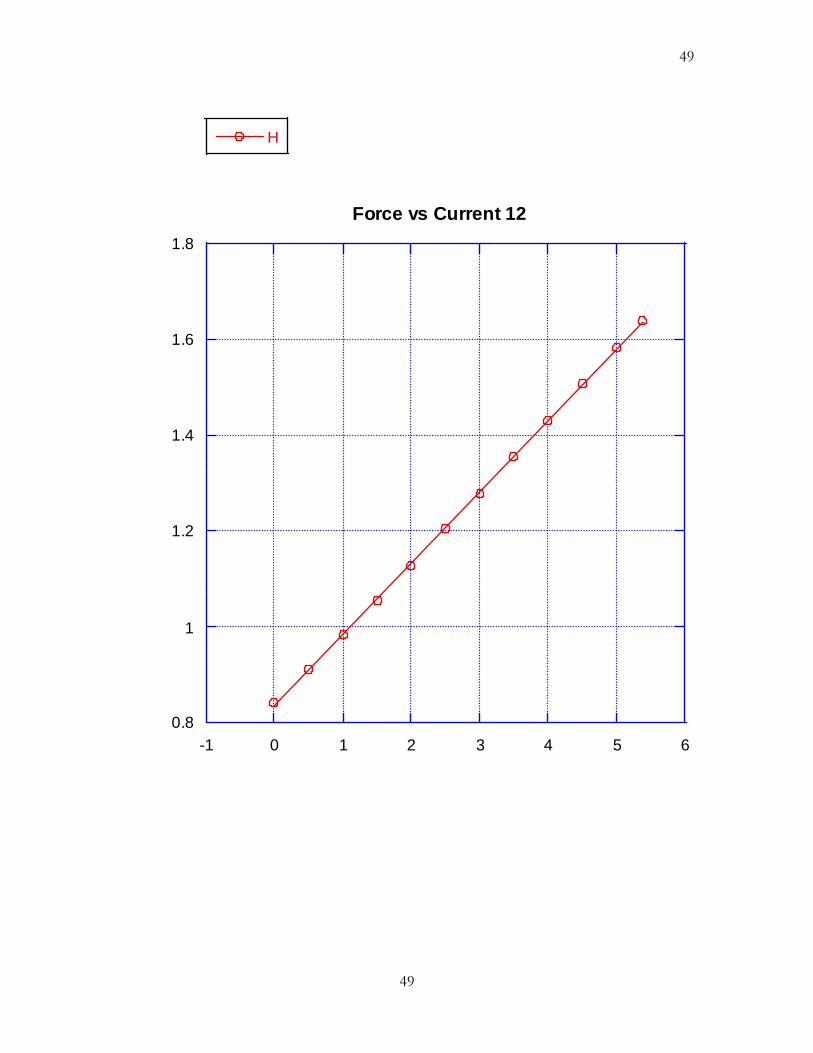
0.8
1
1.2
1.4
1.6
1.8
-1 0 1 2 3 4 5 6
Force vs Current 12
H
49

50
0.6
0.8
1
1.2
1.4
1.6
-1 0 1 2 3 4 5 6
Force vs Current 13cm
E
50
51
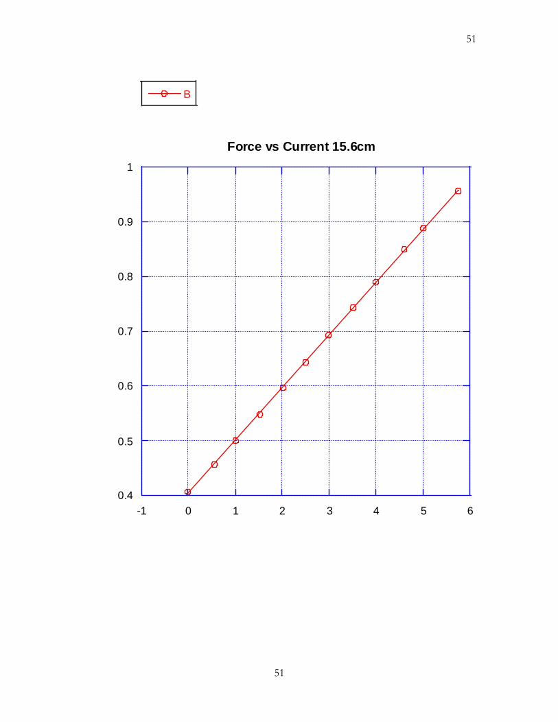
0.4
0.5
0.6
0.7
0.8
0.9
1
-1 0 1 2 3 4 5 6
Force vs Current 15.6cm
B
51

52
0
0.5
1
1.5
2
2.5
3
3.5
6 8 10 12 14 16
Data 15
B
y = 205.15 * x^(-2.2371) R= 0.99922
B
A
y = m1/m0^ 2.25ErrorValue
3.116206.52m1 NA0.014766ChisqNA0.99872R
52

53
NEODYMIUM MAGNET PROPERTIES:
-0.3
-0.2
-0.1
0
0.1
0.2
0.3
0.4
0.5
-0.05 0 0.05 0.1 0.15 0.2 0.25
Radial Falloff
B
B (T
esla
)
r (m)
y = m1*exp(-m2*M0)-m4*exp(-m...ErrorValue
1.42831.4915m1 83.672124.47m2 23.42253.143m3 1.42831.0694m4
NA0.0016324ChisqNA0.99697R
53

54
10-5
0.0001
0.001
0.01
0.1
1
-0.2 0 0.2 0.4 0.6 0.8 1 1.2
Height Data
B (Tesla)
B (T
esla
)
h (m)
54

55
10-5
0.0001
0.001
0.01
0.1
1
-0.2 0 0.2 0.4 0.6 0.8 1 1.2
Height Data
B (Tesla)E
B (T
esla
)
h (m)
Figure 17
Neodymium Magnetic Field (h=0 at surface, N+) in Tesla:
( )( )
124.5 53.145
5/ 44 2
.7170( , ) 12.83 10
5.589 10
r re eB r h
h
− −−
−−
−= ×
× +
55

56
SOLENOID PROPERTIES AT 4.5A:
0.0001
0.001
0.01
0.1
1
-0.2 0 0.2 0.4 0.6 0.8 1 1.2
4.5A B-Field
B (Tesla)
B (T
esla
)
h (m)
y = m1*(M0 2+m2 2)^(-m3)ErrorValue
1.5688e-59.5242e-5m1 0.00134190.030463m2
0.0388811.2321m3 NA6.2592e-7ChisqNA1R
Falloff of solenoid at 4.5 A.
Vmax Min Nat Freq Width Guage Resistancs (Ohms)
12.339 0.00033763 4.1534 10.000 3.0175
15.439 0.00026766 3.2906 11.000 3.8063
19.358 0.00021238 2.6115 12.000 4.7971
24.338 0.00016838 2.0736 13.000 6.0507
30.618 0.00013357 1.6435 14.000 7.6276
56

57
38.558 0.00010592 1.3042 15.000 9.6183
48.594 8.3978e-05 1.0323 16.000 12.132
61.244 6.6599e-05 0.82084 17.000 15.297
77.195 5.2820e-05 0.64964 18.000 19.288
97.317 4.1890e-05 0.51552 19.000 24.321
122.67 3.3227e-05 0.40960 20.000 30.661
154.69 2.6348e-05 0.32481 21.000 38.667
195.04 2.0896e-05 0.25806 22.000 48.756
57

58
DATA SHEETS:
58

59
59
60
60

61
61
62
62

63
63

64
64

65
65
66
66