search for additive nonlinear time series causal models

Journal of Machine Learning Research 9 (2008) 967-991 Submitted 9/06; Revised 9/07; Published 5/08

Search for Additive Nonlinear Time Series Causal Models

Tianjiao Chu [email protected]

Department of Obstetrics, Gynecology & Reproductive SciencesUniversity of Pittsburgh204 Craft Ave., Room B409Pittsburgh, PA 15213, USA

Clark Glymour [email protected]

Department of PhilosophyCarnegie Mellon UniversityPittsburgh, PA 15213, USA

Editor: Greg Ridgeway

AbstractPointwise consistent, feasible procedures for estimating contemporaneous linear causal structurefrom time series data have been developed using multiple conditional independence tests, but nosuch procedures are available for non-linear systems. We describe a feasible procedure for learninga class of non-linear time series structures, which we call additive non-linear time series. We showthat for data generated from stationary models of this type, two classes of conditional independencerelations among time series variables and their lags can be tested efficiently and consistently us-ing tests based on additive model regression. Combining results of statistical tests for these twoclasses of conditional independence relations and the temporal structure of time series data, a newconsistent model specification procedure is able to extract relatively detailed causal information.We investigate the finite sample behavior of the procedure through simulation, and illustrate theapplication of this method through analysis of the possible causal connections among four oceanindices. Several variants of the procedure are also discussed.

Keywords: conditional independence test, contemporaneous causation, additive model regression,Granger causality, ocean indices

1. Introduction

For stationary time series of four or more dimensions, Swanson and Granger (1997) proposed todetermine contemporaneous causation—causal influences occurring more rapidly than the samplinginterval of the time series data—by regressing each time series variable on all lags of all variablesconsidered and using the residuals to test for vanishing partial correlations. Using search proceduresfor directed acyclic graphical linear models, in particular, the PC algorithm (Spirtes et al., 2000),Bessler et al. (2002), Demiralp and Hoover (2003), and Hoover (2005) generalized Swanson andGranger’s procedure to allow specification searches for contemporaneous linear systems among allpartial orderings of the dependencies among the variables. Moneta (2003) derived the correctionneeded for the fact that the correlations are obtained from residuals of a regression, and applied it toa set of cointegrated variables.

All these methods are designed for linear systems with joint Normal distributions, and allowneither unrecorded (latent) common causes nor feedbacks. One source of these limitations is the

c©2008 Tianjiao Chu and Clark Glymour.

CHU AND GLYMOUR

search algorithm used by all of these procedures, PC, which is known to be consistent only in theabsence of feedback relations and latent common causes. In principle, some of these difficultiescan be met by replacing PC with related algorithms: the FCI algorithm (Spirtes et al., 2000), whichallows latent variables, or an algorithm due to Richardson and Spirtes (1999) that allows linearfeedback relations, though no algorithm is available that is consistent for search for linear causalmodels when both latent variables and feedback may be present.

More fundamentally, PC and related algorithms require conditional independence informationabout the random variables as input, and are therefore limited to distribution families for whichconditional independence tests of arbitrary order are available, such as Multinomial and Normaldistributions. (Another group of causal inference algorithms that are based on model scores, suchas Bayesian posteriors, are unable to handle either latent variables or feedbacks, except under ex-tra constraints (Silva et al., 2006; Drton et al., 2006). For non-Gaussian linear models with latentvariables, independent component analysis based algorithms (Hoyer et al., 2006) could be moreinformative than PC and FCI.) Extending the PC and related algorithms based on conditional inde-pendence constraints to a larger class of systems that includes nonlinear continuous models requiresmore general conditional independence tests. We begin by considering some of the difficultiesinvolved with finding such tests.

In theory, using nonparametric density estimation, we can test conditional independence forany set of random variables which have a joint density with respect to the Lebesgue measure. Forexample, let the joint density of {X ,Y,Z} be fXY Z(x,y,z), the joint density of {X ,Z} be fXZ(x,z),the joint density of {Y,Z} be fY Z(y,z), and the marginal density of Z be fZ(z). We could test ifX and Y are independent given Z by testing if the Hellinger distance between fXY Z(x,y,z) fZ(z)and fXZ(x,z) fYZ(y,z) is 0. For example, Su and White (2007) propose a conditional independencetest for stationary time series satisfying certain conditions, based on a weighted Hellinger distancebetween fX |Y Z(x;y,z) and fX |Z(x;z), where fX |Y Z(x;y,z) and fX |Z(x;z) are densities of the conditionaldistributions of X given {Y,Z} and Z respectively. However, this approach requires nonparametricdensity estimation of multivariate distributions, which is subject to the curse of dimensionality: asthe number of variables increases, the data points become sparse rapidly in the space spanned bythe variables.

Baek and Brock (1992) and Hiemstra and Jones (1994) proposed a nonparametric method in-tended for Granger causality testing of nonlinear time series. Consider a bivariate time series{Xt ,Yt}, t = 1, · · ·, let X

mt = (Xt , · · · ,Xt+m−1) for some m, they proposed to test if X

mt and Y

bt−b

are independent given Xat−a by testing the following null hypothesis:

P(

‖Xmt −X

ms ‖∞ < e | ‖Xa

t−a−Xas−a‖∞ < e, ‖Y b

t−b−Yb

s−b‖∞ < e)

= P(

‖Xmt −X

ms ‖∞ < e | ‖Xa

t−a−Xas−a‖∞ < e

)

.

Unfortunately, only under some specific conditions is the above null hypothesis equivalent tothe hypothesis that X

mt is independent of Y

bt−b given X

at−a (Diks and Panchenko, 2006).

Bell et al. (1996) considered additive model regression (Hastie and Tibshirani, 1990) for condi-tional independence tests in their study of nonlinear Granger causality. An additive model assumesthat the response variable Y is a linear combination of univariate smooth functions of predictorsX = {X1, · · · ,Xp} plus an independent error term. That is:

968

ADDITIVE NON-LINEAR TIME SERIES CAUSAL INFERENCE

Y =p

∑i=1

fi(Xi)+ ε (1)

where it is possible that fi(Xi) = 0 for some i ∈ {1, · · · , p}. Assuming Equation (1), additive modelregression could be used to test if the response variable Y and some predictors Xa ⊆X are inde-pendent conditional on the other predictors Xb = X \Xa, because Y is independent of Xa givenXb if and only if E[Y |X] is constant in Xa}.

Additive regression works well as a conditional independence test in the study of Grangercausality when no contemporaneous causation is allowed among time series, because the only typeof conditional independence relations to be tested is the one described above. For example, in Bellet al. (1996), two additive models were fitted: one model for estimating the conditional expectationof a variable XT+1 given its T lags {X1, X2, · · ·, XT}, another for conditional expectation of XT+1

given {X1, X2, · · ·, XT} and {Y1, Y2, · · ·, YT}. The F test was used to compare these two regressionmodels: if the test failed to reject the first model, XT+1 was judged independent of {Y1, Y2, · · ·, YT}given {X1, X2, · · ·, XT}.

However, the use of additive model regression as a general purpose nonlinear conditional inde-pendence test is problematic, even for variables that are known to be related via additive models.Generally speaking, it is not always valid to use additive model regression to test conditional in-dependence relations other than those between the response variable and some predictors given theother predictors. First, in some cases, additive model regression may miss some conditional de-pendencies. Consider a causal system with two exogenous variables X1 and X2, and an endogenousvariable Y such that Y = X2

1 + X22 + εY , where X1,X2 and εY are independent Gaussian variables.

Although the predictors X1 and X2 are dependent given the response variable Y , the conditionalexpectation of X1 given Y and X2 estimated using additive model regression will be constant in X2.Second, even worse, in some cases additive model regression may miss some conditional indepen-dencies. Consider a system with two exogenous variables X1 and X2, and five endogenous variablesW = X1 + X2 + εW , Y = W 2 + εY , U = log(X1)+ εU , V = log(X2)+ εV , and Z = U +V + εZ . Al-though the two response variables Y and Z are independent conditional on the predictors X1 and X2,Z will be present in the conditional expectation of Y given {X1,X2,Z} estimated by additive modelregression. (Note that Y contains a term 2X1X2, and eZ = eεU +εV +εZ X1X2.)

Nevertheless, additive model regression has some very attractive features. First, and probablymost importantly, it is not subject to the curse of dimensionality. In fact, Stone (1985) shows that therate of convergence for an additive model regression is the same as that for a univariate smoother,which is much faster than a general multidimensional nonparametric regression method. The secondmajor advantage of additive model regression is that it is possible to identify the contribution of eachpredictor to the response variable, thus allowing an intuitive interpretation of the fitted models.

In the following sections, we define a additive non-linear time series model by imposing lin-ear constraints only among contemporaneous variables. We show that two families of conditionalindependence relations can be tested consistently among variables in a additive non-linear time se-ries model using additive model regression. That is, asymptotically, additive model regression willneither miss any conditional independence relations nor report any spurious conditional indepen-dence relations when applied to data generated from a additive non-linear time series model to testthose two families of conditional independence relations. We propose an inference procedure fornonlinear time series data that requires only information about these two families of conditionalindependence relations.

969

CHU AND GLYMOUR

2. Additive Non-linear Time Series Models

Below we present the definition of a family of nonlinear time series models for which additive modelregression based conditional independence test is possible. Here Xt is a p dimensional observedtime series, Ut a q dimensional unobserved time series, and εt a p dimensional white noise.Definition: A p dimensional time series {X}t = {· · ·, X1, · · ·, XT , · · ·}, where Xt = {Xt,1, · · · ,Xt,p},is generated from a lag T additive non-linear model if it satisfies the following conditions:

C1 For i = 1, · · · , p,

Xt,i = ∑1≤ j≤p, j,i

c j,iXt, j + ∑1≤k≤p,1≤l≤T

fk,i,l(Xt−l,k)+q

∑m=1

bm,iUt,m + εt,i (2)

where bm,i’s and c j,i’s are constants, and fk,i,l’s are smooth univariate functions

C2 · · · ,ε1,1, · · · ,ε1,p,ε2,1, · · · ,εt,i, · · · and · · · ,U1,1, · · · ,U1,q,U2,1, · · · ,Ut, j, · · · are jointly indepen-dent, with εt,i ∼ N(0,σ2

1,i) and Ut, j ∼ N(0,σ22, j).

C3 There is a k and an i such that fk,i,T (·) , 0

C4 There is no sequence of indices { j1, j2, · · · , jm} such that c j1, j2 , c j2, j3 , · · ·, c jm−1, jm , c jm, j1 areall nonzero.

The model is additive because Equation (2) includes both linear terms and arbitrary smoothterms. It is also recursive in the sense that given an initialization of Xt−T , · · · ,Xt−1, all the laterpoints in the time series, starting from Xt , can be generated inductively.

A additive non-linear model can be causally interpreted in the following way:

• Xt, j is a direct cause of Xt,i if and only if c j,i , 0 in Equation (2), (for the definition of directcause, see Spirtes et al., 2000; Pearl, 2000);

• Xt−l, j is a direct cause of Xt,i if and only if f j,i,l(·) , 0 in Equation (2);

• Latent common causes are allowed only for variables in the same time tier, and Xt,i and Xt, j

have a latent common cause Ut,m if and only if there is an m such that bm,ibm, j , 0.

Note that both Ut and εt are multi-dimensional Gaussian white noise and both are unobserved.However, for i = 1, · · · , p, εt,i can only be a direct cause of Xt,i, where for m = 1, · · · ,q, Ut,m

can be a direct cause of several variables in Xt .

• Condition C4 means that no contemporaneous feedback is allowed. If condition C4 is vio-lated, Xt, jm would be a direct cause of Xt, j1 , while at the same time Xt, j1 would be a (possiblyindirect) cause of Xt, jm .

Note that using results of Richardson and Spirtes (1999) the method described in Section 3can be modified to allow contemporaneous feedback.

A additive non-linear model can be represented by a directed graph consisting of nodes forXT+1,1, · · · ,XT+1,p and their direct causes, and directed edges between nodes for the direct influencesbetween the corresponding variables. We call this graph a unit causal graph for the corresponding

970


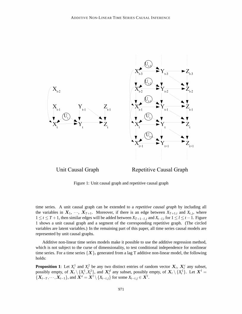
Figure 1: Unit causal graph and repetitive causal graph

time series. A unit causal graph can be extended to a repetitive causal graph by including allthe variables in X1, · · ·, XT+1. Moreover, if there is an edge between XT+1,i and Xt, j, where1≤ t ≤ T +1, then similar edges will be added between XT+1−l, j and Xt−l,i for 1≤ l ≤ t−1. Figure1 shows a unit causal graph and a segment of the corresponding repetitive graph. (The circledvariables are latent variables.) In the remaining part of this paper, all time series causal models arerepresented by unit causal graphs.

Additive non-linear time series models make it possible to use the additive regression method,which is not subject to the curse of dimensionality, to test conditional independence for nonlineartime series. For a time series {X}t generated from a lag T additive non-linear model, the followingholds:

Proposition 1: Let X1t and X2

t be any two distinct entries of random vector Xt , Xct any subset,

possibly empty, of Xt \ {X1t ,X2

t }, and Xdt any subset, possibly empty, of Xt \ {X1

t }. Let Xl =

{Xt−T , · · · ,Xt−1}, and Xe = X

l \{Xt−i, j} for some Xt−i, j ∈Xl .

971

CHU AND GLYMOUR

• For any xdt and x

l , conditional on Xdt = x

dt and X

l = xl , X1

t has a normal distributionN(µ1|a,σ2

1|a) such that µ1|a is a linear combination of xdt and smooth univariate functions of

entries of xl , and σ1|a is independent of t, x

l and xdt . Thus, X1

t is independent of Xt−i, j

conditional on Xe and X

dt if and only if µ1|a, the conditional expectation of X 1

t given Xdt =

xdt and X

l = xl , is constant in xl, j.

• For any x2t , x

ct and x

l , conditional on X2t = x2

t , Xct = x

ct , and X

l = xl , X1

t has a normaldistribution N(µ1|b,σ2

1|b) such that µ1|b is a linear combination of x2t , xc

t , and smooth univariate

functions of entries of xl , and σ1|b is constant in t, x2

t , xct , and x

l . Thus, X1t is independent

of X2t conditional on X

ct and X

l if and only if, µ1|b, the conditional expectation of X 1t given

X2t = x2

t , Xct = x

ct , and X

l = xl , is constant in x2

t .

Proposition 1 implies that it is possible to use additive model regression to test the following twotypes of conditional independence relations among variables in a additive non-linear model. First,we can test if X1

t and X2t are independent conditional on X

ct and X

l by estimating the conditionalexpectation of X1

t given {X2t } ∪X

ct ∪X

l using additive model regression, and check if X 2t is a

significant predictor for X1t using statistical tests such as the F test (Bell et al., 1996) or the BIC

scores (Huang and Yang, 2004). Similarly, if Xt−i, j is not a significant predictor for X 1t in the additive

model regression of X1t against X

l and Xdt , we would say X1

t and Xt−i, j are independent conditionalon X

dt and X

e.To make the above tests valid, we also need the assumption that additive model regression

is an (asymptotically) consistent estimator of conditional expectations such as E[X 1t |X

dt ,X l] and

E[X1t |X

2t ,Xc

t ,X l]. Fortunately, it has been shown that, given a stationary nonlinear time series{X}t , nonparametric estimation of the conditional mean E[Xt |Xt−1, · · · ,Xt−T ] is asymptoticallyconsistent and/or asymptotically normal, provided certain conditions are satisfied (Robinson, 1983;Truong and Stone, 1992; Chen and Tsay, 1993; Tjøstheim and Auestad, 1994; Hardle et al., 1997;Cai and Masry, 2000; Huang and Yang, 2004). Generally speaking, besides some regularity condi-tions on the density of Xt ∪X

l and smoothness condition on E[Xt |Xl], {X}t should satisfy some

form of α mixing condition. {X}t is α mixing if for some α(n)→ 0,

sup{|P(A∩B)−P(A)P(B)| : A ∈ Ft ,B ∈ Gn+t} ≤ α(n)

where Ft is the σ-field generated by Xt ,Xt−1, · · ·, and Gn+t the σ-field generated by Xt+n,Xt+n+1,· · · .

A concept closely related to α mixing is geometric ergodicity. A stationary time series {X}t isgeometrically ergodic if there is a function M(x) < ∞ and a constant ρ < 1 such that for all x:

supA|P(Xn ∈ A|X0 = x)−π(A)| ≤M(x)ρn

where π is the stationary distribution of {X}t . For stationary time series, geometric ergodicityimplies α mixing for an α(n) of exponential rate (Davydov, 1973). Sufficient conditions for anonlinear time series to be geometrically ergodic can be found in Chan and Tong (1994), An andHuang (1996), and Cline and Pu (1999). In particular, Xia and An (1999) provides a set of sufficientconditions for the geometric ergodicity of time series generated by projection pursuit models, ofwhich our additive non-linear model is a special case.

972


3. A Causal Inference Algorithm

Consider a time series {X}t = {X1, · · · ,Xt , · · ·} are generated from a lag T additive non-linearmodel. Let X

l = {Xt−1, · · · ,Xt−T}, X1t and X2

t be any two entries of Xt , Xbt be any subset, possi-

bly empty, of Xt \{X1t }, X

ct be any subset, possibly empty, of Xt \{X1

t ,X2t }, Xt−i, j any variable in

Xl , and X

e = Xl \{Xt−i, j}. Using additive model regression, we can test two types of conditional

independence relations: 1), if X 1t and X2

t are independent given Xct and X

l , and 2), if X1t and Xt−i, j

are independent given Xbt and X

e. These pieces of information are not generally sufficient forcurrently available causal inference algorithms, such as the PC and FCI, to be informative: theseprocedures require (in the worst case) complete conditional independence information. However,starting from the same principle behind the PC and FCI algorithms, we describe a procedure thatrequires only these two types of conditional independence information. The procedure, which is ca-pable of producing very informative causal structures, takes advantage of the constraints on possiblecausal relations among the random variables imposed by additive non-linear models, for example,Xt2,k cannot be a cause of Xt1, j if t1 < t2, no latent common cause exists for Xt2,k and Xt1, j if t1 , t2,etc.

The following propositions are needed to justify our procedure. We assume familiarity withnotions from the graphical modeling literature, including the notion of d-separation (Pearl, 2000),and faithfulness (Spirtes et al., 2000). In summary:

Formally a causal graph G is defined as an ordered pair 〈V ,E〉, where V is the set of variablesin G, and E the set of edges in G. An edge e in E is again defined as an ordered pair 〈Vi,Vj〉,where Vi and V j are two variables in V . Given an edge e = 〈Vi,Vj〉 in graph G, we say that Vi is adirect cause of V j in G. The subgraph Gm induced by Vm, where Vm is a subset of V , is definedas an ordered pair 〈Vm,En〉 such that an edge e = 〈Vi,Vj〉 is in En if and only if e is in E and thetwo variables {Vi,Vj} are both in Vm. A vertex is a collider on an undirected path in a directedacyclic graph (DAG) if and only if it is the second member of both of two edges on the path, thatis, two edges on the path are directed into it. Two vertices X , Y (representing random variables)are d-separated with respect to a set Z of vertices if and only if every undirected path between thevariables contains a collider having no directed path into a member of Z or contains a non-colliderthat is a member of Z. A joint distribution on the variables (vertices) of a DAG is faithful if andonly if all conditional independence relations follow from the d-separation property applied to theDAG.

In the three propositions below, {X1, · · · ,Xt , · · ·} form a time series generated from a lag Tadditive non-linear model, X

l = {Xt−1, · · · ,Xt−T}, X1t and X2

t are any two entries of Xt , andX

e = Xl \{Xt−i, j} for some Xt−i, j ∈X

l

Proposition 2: The d-separation relations among the variables in Xt conditional on Xl in a repet-

itive causal graph Gc are the same as the d-separation relations among the variables in Xt in thesubgraph of Gc induced by Xt .

Proof: See Moneta (2003), proposition 4. �

Proposition 3: Consider a time series {X}t = {X1, · · · ,Xt , · · ·} generated from a lag T additivenon-linear model. Let X

l = {Xt−1, · · · ,Xt−T}, X1t and X2

t be any two entries of Xt . Assumingfaithfulness, if there is a variable Xt−i, j ∈X

l such that X2t and Xt−i, j are independent conditional on

Xe = X

l \{Xt−i, j}, but Xt−i, j and X1t are not independent conditional on X

e, then X1t is not a cause

of X2t .

973

CHU AND GLYMOUR

Proof: Suppose X1t is a cause of X2

t , then there must be a directed path P′ from X1t to X2

t suchthat each vertex on P′ is in Xt . If Xt−i, j and X1

t are dependent given Xe, there must be a path P

d-connecting Xt−i, j and X1t given X

e. Thus, no variable in Xe is a non-collider on path P, and all

the colliders on path P must be observed ancestors of Xe, hence must be in X

e. (Note that theset of observed ancestors of X

e is either Xe or X

e ∪{Xt−i, j}). This implies that P must be intoX1

t , because otherwise either P would be a direct path from X 1t to Xt−i, j, which is not allowed, or

there must be a collider on P that is both a descendant of X 1t and an element of X

e, which also isimpossible. By appending the direct path P′ to P, we get a path d-connecting Xt−i, j and X2

t givenX

e, which is a contradiction. �Proposition 4: Consider a time series {X}t = {X1, · · · ,Xt , · · ·} generated from a lag T additivenon-linear model. Let X

l = {Xt−1, · · · ,Xt−T}, X1t be any entry of Xt , Xt−i, j be any variable in X

l ,X

dt be the set of all observed contemporary direct causes of X 1

t , and Xe = X

l \{Xt−i, j}. Assumingfaithfulness, Xt−i, j and X1

t are dependent conditional on Xdt and X

e if and only if:

• either Xt−i, j is a direct cause of X1t ,

• or there is a path P between X 1t and Xt−i, j, with 〈W1, · · ·, Wm〉 being the set of observed

variables on P between X1t and Xt−i, j and ordered along the direction from X 1

t to Xt−i, j, suchthat:

1. Wi ∈Xt for i = 1, · · · ,m;

2. X1t and W1 have a latent common cause;

3. if Wi ∈Xdt then Wi is a collider on P;

4. Wi is a (possibly indirect) cause of X 1t for i = 1, · · · ,m;

5. Xt−i, j is a direct cause of Wm.

Proof: The if part of the proposition is trivial, here we only prove the only if part.Suppose Xt−i, j is not a direct cause of X1

t , then there is a path P d-connecting Xt−i, j and X1t

conditional on Xdt and X

e. Let W = 〈W1, · · · ,Wm〉 be the set of observed variables on P betweenX1

t and Xt−i, j, ordered along the direction from X 1t to Xt−i, j.

To show that Wi ∈Xt for i = 1, · · · ,m, we note that if W j is the first element in W such thatWj <Xt , it must belong to X

e, where W j−1 is in Xt . Because there is no observed variable betweenWj−1 and W j on P, by the definition of additive non-linear models, there must be a direct edge fromWj to Wj−1 on P (let X1

t =W0 when j = 1). This means that W j is not a collider on P, hence P cannotd-connect X1

t and Xt−i, j conditional on Xe and X

dt , which contradicts our assumption. Using the

same argument, given that Wm ∈Xt , it is easy to see that Xt−i, j must be a direct cause of Wm.Next we show that W1 and X1

t must have a latent common cause. Assume that there is no latentcommon cause for W1 and X1

t . Because there is no observed variable between W1 and X1t on P, they

must be adjacent on P, hence there must be a direct causal relation between X 1t and W1. Consider

the two alternative cases:

• First, suppose that W1 is a direct cause of X1t . Then W1 ∈X

dt , and is a non-collider on P,

hence P cannot d-connecting Xt−i, j and X1t conditional on X

dt and X

e.

974


• Second, suppose X1t is a direct cause of W1. Then there must be a variable Wi for some

i ≥ 1 such that the subpath {X 1t ,W1, · · · ,Wi} of P is a directed path from X 1

t to Wi, and Wi

is a collider on P. This would imply that Wi has to be a cause of X1t , for otherwise neither

Wi nor any of its descendants belong to Xdt , which means that P cannot d-connect X 1

t andXt−i, j conditional on X

e and Xdt . But allowing Wi to be a cause of X1

t would make the pathX1

t ,W1, · · · ,Wi,X1t a directed cycle, which is impossible.

It is obvious that if Wi ∈Xdt , then it must be a collider on P. To show that Wi is a cause of X1

t ,we note that if W j is a collider on P, it must be a cause of X 1

t , for otherwise neither W j nor any ofits descendants belongs to X

dt , hence P cannot d-connect X 1

t and Xt−i, j conditional on Xe and X

dt .

Therefore Wi must be a cause of X1t , because it is either a collider on P, or a cause of a collider on

P. �Given propositions 2, 3, and 4, we propose a three-step procedure for inference to unit causal

graphs from time series data generated by additive non-linear models. The output of this causalinference procedure is a Partial Ancestral Graph (PAG). Roughly speaking, a PAG is a graph con-sisting of a list of vertices representing observed random variables, and 3 types of end points, −,◦, and >, which are combined to form the following 4 types of edges representing causal relationsbetween random variables.

• X → Y means that X is a (possibly indirect) cause of Y .

• X ↔ Y means that there is a latent variable Z that is a (possibly indirect) cause of both X andY .

• X �→ Y means either X → Y or X ↔ Y .

• X�Y means either X →Y , or Y �→ X . In other words, X�Y means that X and Y cannotbe d-separated by any other observed variables.

For detailed explanation of PAGs, see Spirtes et al. (2000). Following Spirtes et al. (2000), wealso use * as a meta symbol to represent any of the three end points.

Below is a constraint based additive non-linear time series causal inference procedure for non-linear time series with latent common causes. The conditional independence information requiredby the procedure can be obtained using additive model regression based conditional independencetests mentioned in the previous section. Here we assume that the time series data satisfies variousconditions for the asymptotic consistency and normality of the additive model estimator, and that anupper bound Tmax on the unknown true lag number T of the additive non-linear model has been set,either using the procedures in Tjøstheim and Auestad (1994) or Huang and Yang (2004), or based onbackground knowledge. So long as Tmax is no less than T , the following procedure asymptoticallyobtains a correct PAG. Of course, choosing a Tmax much higher than T will reduce the efficiency ofthe procedure.

The symbols in the following procedure are defined in the same way as in the beginning of thissection, except that X

l is redefined as Xl = {Xt−1, · · · ,Xt−Tmax}.

1. Identify contemporary causal relations

(a) For all choices of X1t , X2

t , and Xct , determine if X1

t is independent of X2t conditional on

Xct and X

l .

975

CHU AND GLYMOUR

(b) Treat the above conditional independence relations as if they were conditional indepen-dence relations between X 1

t and X2t given X

ct .

• Feed these conditional independencies to a causal inference algorithm allowingpresence of latent common causes, such as the FCI algorithm. Derive the PAG forthe contemporary causal structure among variables in Xt . Call this PAG πt .

• For all choices of X1t , identify the set of possible contemporaneous direct causes

of X1t , where X2

t is a possible contemporaneous direct cause of X 1t if in πt either

X2t �( X1

t , or X2t �→ X1

t , or X2t → X1

t . Denote by PCDC(X1t ) the set of possible

contemporaneous direct causes of X 1t .

2. Identify lagged causal relations.

(a) Create a new graph π f such that the vertices in π f are {Xt ,Xt−1, · · · ,Xt−T}, and theedges in π f are exactly the same as the edges in πt .

(b) For all choices of X1t , Xt−i, j, and X

bt , determine if X1

t and Xt−i, j are independent givenX

e and Xbt

• For all choices of X1t , identify the set of possible lagged direct causes of X 1

t , wherea lagged variable Xt−i, j is a possible lagged direct cause of X 1

t if for all Xdt ⊆

PCDC(X1t ), Xt−i, j and X1

t are dependent given Xdt and X

e. Denote by PLDC(X1t )

the set of possible lagged direct causes of X 1t

• For all choices of X1t , identify the set of permanent lagged predictors of X 1

t , whereXt−i, j is a permanent lagged predictor of X 1

t if for all Xbt ⊆ (Xt \ {X1

t }), Xt−i, j

and X1t are dependent given X

bt and X

e. Denote by PLP(X1t ) the set of permanent

lagged predictors of X1t

(c) Add edges representing the lagged causes of each variable in Xt to π f :

i. For all choices of X1t , add an edge Xt−i, j→ X1

t to π f if Xt−i, j ∈ PLP(X1t ).

ii. For all choices of X1t , add an edge Xt−i, j → X1

t to π f if Xt−i, j ∈ PLDC(X1t ), and

Xt−i, j is not adjacent to any other variable in π f .

3. Orient the contemporary PAG according to the following rule:

(a) Repeat the following procedure until no more changes can be made to π f .

i. If Xt−i, j→ X1t �∗X

2t is in π f , and Xt−i, j and X2

t are not adjacent, then:If Xt−i, j and X2

t are independent given Xe, but dependent given X 1

t and Xe, then

orient the edge between X 1t and X2

t as X1t ←∗X

2t

ii. If Xt−i, j→ X1t �∗X

2t is in π f , and Xt−i, j and X2

t are not adjacent, then:If Xt−i, j and X2

t are dependent conditional on Xe, but independent conditional on

X1t and X

e, then orient the edge between X 1t and X2

t as X1t → X2

t

(b) Apply the orientation step of FCI algorithm to further orient the contemporary PAG π f .

Proposition 2 provides justification for the first step in this procedure, proposition 3 the thirdstep. Proposition 4 is needed for the second step, as we can see that the set of contemporaneousdirect causes of a variable X 1

t is a subset of PCDC(X1t ), thus by proposition 4 we have:

976


Lagged direct causes of X1t ⊆ PLP(X1

t )⊆ PLDC(X1t ) ⊆ Lagged causes of X1

t

Note that step 2(c) is designed to make the procedure more robust.

The complexity of the above procedure is primarily determined by step 1(a), where k2k−1 addi-tive model regressions are performed to test the conditional independence relations required by thelater steps.

We want to emphasize that the above procedure can be modified in various ways to accommo-date changes in the assumptions about the time series data generating models. In the last section(Section 6) of this paper, we discuss in details about different extensions of the above procedure.

4. Simulation Study

In this section, we conduct a simple simulation study to evaluate the performance of the additivenon-linear causal inference algorithm presented in Section 3. In particular, we would like to seeif the additive non-linear algorithm can provide a viable solution to the problem of nonlinear timeseries causal inference. For comparison, we also apply a causal inference procedure designed forlinear time series to the simulated data. Because there is no currently available efficient automatedcausal inference algorithm for linear time series with contemporaneous causal relations, the linearprocedure used for comparison actually is an extension of our additive non-linear causal inferenceprocedure under the assumption that the time series data are generated from linear models. (Bessleret al. 2002, Demiralp and Hoover 2003, Moneta 2003 and Hoover 2005 discussed efficient waysof identifying the contemporaneous causal pattern, that is, the Markov equivalence classes (MEC)of the causal graphs for contemporaneous variables assuming causal sufficiency. However, theirprocedures are not complete because, when the MEC consists of multiple contemporaneous causalgraphs, these procedures all require further background information to uniquely identify the con-temporaneous causal graph before proceeding to derive the causal pattern for both contemporaneousand lagged variables. Oxley et al. (2004) provides a less efficient algorithm for linear time seriesthat treats a k-dimensional lag p structural vector autoregressive model (SVAR(p)) as a linear causalmodel with k(p+1) variables.) The linear procedure differs from the additive non-linear algorithmonly in step 1: unlike the original algorithm which uses additive regression to test conditional inde-pendence, the linear procedure uses linear regression instead.

We use the Mersenne Twister algorithm implemented in java package RngPack (version 1.1a)for random number generation, and the gam function in the R package gam (version 0.97) for addi-tive model regression.

The simulated data are generated from the four causal structures shown in Figure 2. Note thatin this simulation study the true PAGs happen to have no circles, and can be represented by thesame graphs in Figure 2. The chain-like contemporaneous causal structure is chosen to evaluatethe ability of our algorithm to identify the direction of those contemporaneous causal relations thatcould not be detected using previous algorithms (Bessler et al., 2002; Demiralp and Hoover, 2003;Moneta, 2003; Hoover, 2005). For each causal structure, we consider the following four types ofmodels, characterized by the type of functional relations between an effect variable and its directcauses:

977

CHU AND GLYMOUR

Figure 2: Causal graphs and true PAGs of simulation data

• Trigonometric lag models: Each contemporaneous variable is a linear combination of othercontemporaneous variables and univariate trigonometric functions of lagged variables. Forexample, in one model, we have:

Yt = 0.5Xt + sin(2Yt−1)− cos(10Zt−2)+ εY .

• Polynomial lag models: Each contemporaneous variable is a linear combination of othercontemporaneous variables and univariate polynomial functions of lagged variables. For ex-ample, in one model, we have:

Yt = 0.5Xt +0.3Y 2t−1−0.1Z3

t−2 + εY .

• Linear lag models: Each contemporaneous variable is a linear combination of other contem-poraneous variables and lagged variables. For example, in one model, we have:

Yt = 0.5Xt +0.3Yt−1−0.1Zt−2 + εY .

• Trigonometric contemporaneous models: Each contemporaneous variable is a linear combi-nation of univariate trigonometric functions of other contemporaneous variables and laggedvariables. For example, in one model, we have:

Yt = cos(Xt)+ sin(2Yt−1)− cos(10Zt−2)+ εY .

978


Note that these models do not belong to the family of additive non-linear time series models,for they violate the assumption C1.

In total we have 16 data generating models, with 12 of them being additive non-linear timeseries models (including 4 linear time series models). For each of the 16 models, we generate 4random time series data sets of length 200, 500, 1000, and 2000 respectively. For each data set, werun both the additive non-linear procedure and the linear procedure. The upper bound Tmax of thetrue lag number T is set to 3 for all simulations, (T is equal to 2 for 12 of the data generating modelsbased on casual structure (A), (B), and (C) in Figure 2, and 1 for the other 4 models based on casualstructure (D)). The learned PAGs are compared with the true PAGs, which are also represented bythe graphs in Figure 2.

The additive non-linear procedure presented in Section 3 requires, for each contemporane-ous variable, say Xt , the following two types of conditional independence information: (1) if Xt

is independent of another contemporaneous variable, say Yt , given all the lagged variables L ={Xt−2,Xt−1,Yt−2, Yt−1, Zt−2, Zt−1} and a subset of the remaining contemporaneous variables, say,{Zt}; and (2), if Xt is independent of a lagged variable, say Xt−1, given all the other lagged variablesand a subset of contemporaneous variables, say, {Zt}. These conditional independence relations aretested by checking if E[Xt |L,Zt ] is constant in Yt or Xt−1 respectively. For example, to test if Xt−1 ispresent in E[Xt |L,Zt ], we follow Huang and Yang (2004) by starting from a model A, where Xt isregressed against L and Zt , and searching for a submodel of A with the lowest BIC score. If Xt−1 ispresent in this submodel with lowest BIC score, it is present in E[Xt |L,Zt ]. Otherwise, it is not.

The simulation results are summarized in Figure 3. Each of the four panes in Figure 3 summa-rizes the results of 16 simulated time series data sets generated from the same type of models. Weuse the average error rates to evaluate the performance of the two algorithms. The definitions ofthe various error rates are similar to those in Spirtes and Meek (1995). Consider a p dimensionaltime series data. An edge omission error occurs when two variables are adjacent in the true PAGbut not in the learned PAG. An edge commission error occurs when two variables are adjacent inthe learned PAG but absent in the true PAG.

The edge omission error rate is defined as:

Eo =Number of edge omission errorsNumber of edges in the true PAG

.

The edge commission error rate is defined as:

Ec =Number of edge commission errors

Maximum number of possible edge commission errors.

When inferring causal structure from a p dimensional time series data set, if the upper bound of thetrue lag number is set to Tmax, the maximum number of possible edge commission errors is equal to:

p2Tmax +p(p−1)

2−Number of edges in the true PAG

where p2Tmax + p(p−1)/2 is the maximum number of edges can be found in the unit causal graphfor any p-dimension lag Tmax time series model.

The solid lines in each pane of Figure 3 represent the average omission error rates for differenttime series lengths; the dotted lines represent the average commission error rates. Blue lines with

979

CHU AND GLYMOUR

Trig Contemp

sample size

erro

r ra

te

200 500 1000 2000

0.0

0.2

0.4

0.6

0.8

Trig Lag

sample size

erro

r ra

te

200 500 1000 2000

0.0

0.2

0.4

0.6

0.8

Poly Lag

sample size

erro

r ra

te

200 500 1000 2000

0.0

0.2

0.4

0.6

0.8

Lin Lag

sample size

erro

r ra

te

Edge Omission: SPEdge Omission: LINEdge Commission: SPEdge Commission: LIN

200 500 1000 2000

0.0

0.2

0.4

0.6

0.8

Figure 3: Error rate for edge discovery

circles represent results obtained by the additive non-linear algorithm, red lines with triangles theresults by the linear procedure.

The pane with label “Trig Contemp” gives the results for data generated from the trigonometriccontemporaneous models. We choose these models in the simulation study precisely because theylie outside of the family of additive non-linear time series models, for they violate the functionalassumption (C1) in the definition of additive non-linear time series models. The simulation resultssuggest that, when the assumption C1 is violated, the additive non-linear algorithm can still discovermost of the edges. However, as the length of time series increases, the average number of extra edgesalso increases, apparently because the data generating models are not additive non-linear time seriesmodels. The linear procedure is not satisfactory, missing most of the edges in the true models.

980


The panes labeled with “Trig Lag” and “Poly Lag” show the results for trigonometric lag modelsand polynomial lag models, both of which are genuine additive non-linear time series models. Theadditive non-linear algorithm performs very well for the trigonometric lag models, but less thansatisfactory for polynomial lag models. Its performance for polynomial lag models, however, doesimprove as the length of time series increases. The linear procedure performs poorly in both cases,missing at least half of the edges.

The pane with label “Lin Lag” provides the results for linear lag models. Given that a linearlag model is simply a linear time series model, which is a special case of additive non-linear timeseries model, we expect that both algorithms should perform very well, as they do. This, on the onehand, suggests that the linear procedure is a good choice for linear time series causal inference, onthe other hand, implies that the additive non-linear algorithm does not suffer from overfitting.

We also compare the average error rates for orientation of the edges among contemporaneousvariables by the additive non-linear algorithm and the linear procedure. Suppose Xt and Yt areadjacent in both the learned PAG and the true PAG, an arrowhead omission error occurs if the edgeis oriented as Xt ∗→Yt in the true PAG, but as Xt ∗—Yt or Xt ∗( Yt in the learned PAG. Similarly, anarrowhead commission error occurs if the edge is oriented as Xt —∗ Yt or Xt �∗Yt in the true PAG,but as Xt ←∗Yt in the learned PAG. Let E be the set of edges among contemporaneous variablesin the true PAG such that the pairs of variables connected by these edges are also adjacent in thelearned PAG. The arrowhead omission error rate is defined as:

Ao =Number of arrowhead omission errors

∑e∈E Number of arrowheads in e.

The arrowhead commission error rate is defined as:

Ac =Number of arrowhead commission errors

∑e∈E Number of non-arrowheads in e.

In Figure 4, the solid lines in each pane represent the average arrowhead omission error rates;the dotted lines represent the average arrowhead commission error rates. As in Figure 3, bluelines with circles represent results obtained by the additive non-linear algorithm, red lines withtriangles the results by the linear procedure. (Note that in the top two panels labeled respectivelywith “Trig Contemp” and “Trig Lag”, the lines representing omission error and commission error forthe additive non-linear algorithm overlap. In the bottom two panels labeled respectively with “PolyLag” and “Lin Lag”, the lines representing commission error for the additive non-linear algorithmand the linear algorithm overlap.)

There are two more scores to measure how close a learned PAG is to the true PAG, that is,the tail omission error rate and the tail commission error rate. Suppose Xt and Yt are adjacentin both the learned PAG and the true PAG, a tail omission error occurs if the edge is oriented asXt → Yt in the true PAG, but as Xt �∗Yt in the learned PAG. A tail commission error occurs if theedge is oriented as Xt �∗Yt in the true PAG, but as Xt → Yt in the learned PAG. Note that thesedefinitions are stated so that an arrowhead commission/omission error will not be counted againas a tail omission/commission error. Because there is no circle in the true PAGs in this simulationstudy, we can only compute the tail omission errors for the learn PAGs, shown in Figure 5. The tailomission error rate is defined as:

To =Number of tail omission errors

∑e∈E Number of tails in e.

981

CHU AND GLYMOUR

Trig Contemp

sample size

erro

r ra

te

200 500 1000 2000

0.0

0.2

0.4

0.6

0.8

1.0

Trig Lag

sample size

erro

r ra

te

200 500 1000 2000

0.0

0.2

0.4

0.6

0.8

1.0

Poly Lag

sample size

erro

r ra

te

200 500 1000 2000

0.0

0.2

0.4

0.6

0.8

1.0

Lin Lag

sample size

erro

r ra

te

Arrowhead Omission: SPArrowhead Omission: LINArrowhead Commission: SPArrowhead Commission: LIN

200 500 1000 2000

0.0

0.2

0.4

0.6

0.8

1.0

Figure 4: Error rate for edge orientation: Arrowhead

The additive non-linear algorithm gives excellent results. For example, for the data sets gen-erated from additive non-linear models, that is, the trigonometric lag models, the polynomial lagmodels, and linear lag models, the additive non-linear algorithm makes no arrowhead commissionerrors. The linear procedure performs quite well for polynomial lag models and linear lag models.

Although the scope of this simulation study is very limited, we can get some general idea aboutthe performance of our additive non-linear casual inference algorithm. If we count the number ofvariables in a p dimensional lag T additive non-linear time series model as p(T + 1), then roughlyspeaking, for longer time series, (80 or more observations per variable), the additive non-linearalgorithm outperforms the linear procedure in all situations, including cases where the true model ismore complex than the additive non-linear model and cases where the true model is a linear model.

982


Trig Contemp

sample size

erro

r ra

te

200 500 1000 2000

0.0

0.2

0.4

0.6

0.8

1.0

Trig Lag

sample size

erro

r ra

te

200 500 1000 2000

0.0

0.2

0.4

0.6

0.8

1.0

Poly Lag

sample size

erro

r ra

te

200 500 1000 2000

0.0

0.2

0.4

0.6

0.8

1.0

Lin Lag

sample size

erro

r ra

te

Tail Omission: SP

Tail Omission: LIN

200 500 1000 2000

0.0

0.2

0.4

0.6

0.8

1.0

Figure 5: Error rates for edge orientation: Tail

For shorter time series, (less than 40 observations per variable), the additive non-linear model isstill better in general, but may be not as good as the linear procedure in some cases. Our suggestionis that, for longer time series always choose the additive non-linear algorithm. For shorter timeseries, if computational cost is critical, the linear procedure is a reasonable choice; otherwise westill recommend the additive non-linear algorithm, or better yet, try both of them.

5. Case Study: Ocean Climate Indices

To illustrate the application of the additive non-linear causal inference algorithm for nonlinear timeseries, we use it to study the causal relations among some ocean climate indices.

983

CHU AND GLYMOUR

Climate teleconnections are associations of geospatially remote climate phenomena producedby atmospheric and oceanic processes. The most famous, and first established teleconnection, is theassociation of the El Nino/Southern Oscillation (ENSO) with the failure of monsoons in India. Avariety of associations have been documented among sea surface temperatures (SST), atmosphericpressure at sea level (SLP), land surface temperatures (LST) and precipitation over land areas. Sincethe 1970s data from a sequence of satellites have provided monthly (and now daily) measurementsof such variables, at resolutions as small as 1 square kilometer. Measurements in particular spatialregions have been clustered into time indexed indices for the regions, usually by principal com-ponents analysis, but also by other methods. Climate research has established that some of thesephenomena are exogenous drivers of others, and has sought physical mechanisms for the telecon-nections. We consider here whether constraints on such mechanisms can be obtained by data-drivenmodel selection from time series of ocean indices.

Our data set consists of the following 4 ocean climate indices, recorded monthly from 1958 to1999, each forming a time series of 504 time steps:

SOI Southern Oscillation Index: Sea Level Pressure (SLP) anomalies between Darwin and Tahiti

WP Western Pacific: Low frequency temporal function of the ‘zonal dipole’ SLP spatial patternover the North Pacific.

AO Arctic Oscillation: First principal component of SLP poleward of 20◦ N

NAO North Atlantic Oscillation: Normalized SLP differences between Ponta Delgada, Azores andStykkisholmur, Iceland

To check stationarity, we conduct the augmented Dickey-Fuller (ADF) test. ADF tests for all 4time series reject the null hypothesis that the tested series has a unit root against the alternative thatthe series is stationary, with p values of the tests smaller than 0.01. As a complementary to ADFtests, we also conduct the Kwiatkowski-Phillips-Schmidt-Shin (KPSS) test. For all 4 time series,KPSS tests with lag truncation parameter set to 12 fail to reject the null hypothesis that the testedseries is (trend) stationary against the unit root alternative, with p values of the tests higher than0.1. We also plot the autocorrelations for the 4 time series to check if the data satisfies the strongmixing condition (Figure 6). The idea is that, if a time series satisfies the strong mixing condition,its autocorrelation should decrease rapidly as the lag increases. From the plot, the auto correlationsof SOI do not decrease as quickly as for other indices, but they become insignificant when the lagis above 12 months.

We assume that the 4 indices are generated from a lag 12 additive non-linear model. The choiceof 12 is partly based on the fact that the ocean indices are monthly data. Another concern is thatwith a length of 504, the data would be too sparse for a model with a much longer lag. As in thesimulation study, the R package gam (version 0.97) is used in this analysis. We first remove anylinear trend from the data, then, following the causal inference procedure presented in Section 3,derive a causal structure represented by a PAG for the 4 ocean climate indices. Figure 7 gives thelearned causal structure.

Because of the relative shorter length of the ocean indices data (10 observations per variable fora lag 12 model), it is worth conducting another inference on the 4 ocean indices using the linearprocedure. The resulting causal structure is given in Figure 8.

984


0 5 10 15 20

0.0

0.6

Lag

AC

FSOI

0 5 10 15 20

0.0

0.6

Lag

SOI & NAO

0 5 10 15 20

0.0

0.6

Lag

SOI & AO

0 5 10 15 20

0.0

0.6

Lag

SOI & WP

−20 −15 −10 −5 0

0.0

0.6

Lag

AC

F

NAO & SOI

0 5 10 15 20

0.0

0.6

Lag

NAO

0 5 10 15 20

0.0

0.6

Lag

NAO & AO

0 5 10 15 20

0.0

0.6

Lag

NAO & WP

−20 −15 −10 −5 0

0.0

0.6

Lag

AC

F

AO & SOI

−20 −15 −10 −5 0

0.0

0.6

Lag

AO & NAO

0 5 10 15 200.

00.

6

Lag

AO

0 5 10 15 20

0.0

0.6

Lag

AO & WP

−20 −15 −10 −5 0

0.0

0.6

Lag

AC

F

WP & SOI

−20 −15 −10 −5 0

0.0

0.6

Lag

WP & NAO

−20 −15 −10 −5 0

0.0

0.6

Lag

WP & AO

0 5 10 15 20

0.0

0.6

Lag

WP

Figure 6: Autocorrelation plot for 4 times series

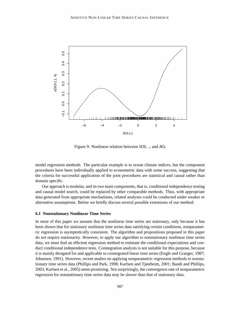
Without a gold standard, it is hard to say which method gives the more accurate informationin this case. But the graph obtained using the linear procedure is likely to miss some nonlineardependencies. For example, an arrow from SOIt−1 to AOt is present in Figure 7, but absent fromFigure 8. It turns out, when regressing AOt against SOIt−1, AOt−1 and NAOt−1 using additive modelregression, the estimated influence of SOIt−1 on AOt is clearly nonlinear (see Figure 9, where thecontribution of SOIt−1 to AOt is plotted as a smooth univariate function of SOIt−1). This is notsurprising given the complexity of the processes represented by the ocean climate indices, and illus-trates the need of causal inference procedures that can be applied to data generated from nonlinearmodels.

6. Discussion

Methods of causal inference, first developed in the machine learning literature, have been success-fully applied to many diverse fields, including biology, medicine, and sociology (Pearl, 2000; Spirteset al., 2000). An essential and distinct feature of these methods is that they require comparativelyless domain knowledge about the system to be studied.

985

CHU AND GLYMOUR

Figure 7: Causal connections among 4 ocean climate indices, using the additive non-linear algo-rithm

Figure 8: Causal connections among 4 ocean climate indices, using the linear procedure

This study extends the application of causal inference to nonlinear time series data. We presenta new procedure that combines semi-automated model search for causal structure with additive

986


−6 −4 −2 0 2 4

−0.

10.

00.

10.

20.

30.

40.

5

SOI.L1

s(S

OI.L

1, 4

)

Figure 9: Nonlinear relation between SOIt−1 and AOt

model regression methods. The particular example is to ocean climate indices, but the componentprocedures have been individually applied to econometric data with some success, suggesting thatthe criteria for successful application of the joint procedures are statistical and causal rather thandomain specific.

Our approach is modular, and its two main components, that is, conditional independence testingand causal model search, could be replaced by other comparable methods. Thus, with appropriatedata generated from appropriate mechanisms, related analyses could be conducted under weaker oralternative assumptions. Below we briefly discuss several possible extensions of our method:

6.1 Nonstationary Nonlinear Time Series

In most of this paper we assume that the nonlinear time series are stationary, only because it hasbeen shown that for stationary nonlinear time series data satisfying certain conditions, nonparamet-ric regression is asymptotically consistent. The algorithm and propositions proposed in this paperdo not require stationarity. However, to apply our algorithm to nonstationary nonlinear time seriesdata, we must find an efficient regression method to estimate the conditional expectations and con-duct conditional independence tests. Cointegration analysis is not suitable for this purpose, becauseit is mainly designed for and applicable to cointegrated linear time series (Engle and Granger, 1987;Johansen, 1991). However, recent studies on applying nonparametric regression methods to nonsta-tionary time series data (Phillips and Park, 1998; Karlsen and Tjøstheim, 2001; Bandi and Phillips,2003; Karlsen et al., 2005) seem promising. Not surprisingly, the convergence rate of nonparametricregression for nonstationary time series data may be slower than that of stationary data.

987

CHU AND GLYMOUR

6.2 Feedback Models

The original definition of additive non-linear models in Section 2 does not allow any feedbackamong contemporaneous variables (see condition C4). To represent mutual influences among con-temporary variables, we can remove condition C4 from the original definition. We also have todrop the U terms in Equation 2 because the currently available algorithm capable of handling feed-backs (Richardson and Spirtes, 1999) does not work in the presence of latent common causes. Theresulting definition defines a additive non-linear feedback model, which, compared to the additivenon-linear model, allows feedback, but not latent common causes. Propositions 1, 2, and 3 still holdfor the new model, proposition 4 needs some modification:Proposition 4’: Let X

bt be the set of all contemporary direct causes of X 1

t . Assuming there is nolatent common cause, Xt−i, j and X1

t are dependent conditional on Xbt and X

e if and only if eitherXt−i, j is either a direct cause of X1

t , or a direct cause of a contemporaneous cause of X 1t .

The only change needed in the causal inference procedure to handle data generated from ad-ditive non-linear feedback models is, in step 1(b), that the FCI algorithm should be replaced by aconsistent causal inference algorithm capable of outputting cyclic graphs, such as the one proposedin Richardson and Spirtes (1999).

6.3 Score Based Search Procedure

The causal inference procedure presented in Section 3 is constraint based. That is, the procedure re-quires explicit conditional independence information as input, (although each conditional indepen-dence constraint is obtained using a BIC score based model selection procedure). As we mentionedin Section 3, the main advantage of this procedure and its modified version is that they can handlethe presence of latent common causes or feedbacks in the contemporaneous causal structure. (Drtonet al. 2006 provides a maximum likelihood estimation algorithm that allows the computation of BICscores for certain types of linear models with correlated error terms, though not for the contempo-raneous causal structure of a additive non-linear model.) If we are willing to exclude feedbacks andlatent common causes, a simple two-step score based procedure can be used to infer causal infor-mation from data generated by additive non-linear models. In the first step, a score based algorithm,such as the GES algorithm (Meek, 1996; Chickering, 2002a,b), is applied to the residuals of additivemodel regression of contemporaneous variables against all lags to obtain a causal pattern represent-ing a Markov equivalence class πt of directed acyclic graphs for the contemporaneous variables. Inthe second step, for each directed acyclic graph G belonging to the Markov equivalence class πt , wegenerate a time series causal model M and compute its BIC score in the following way:

• Each contemporaneous variable X it is regressed against its parents in G and all the lagged

variables Xl . The BIC score method proposed in Huang and Yang (2004) is used to identify

the best submodel (with the lowest BIC score si). The significant predictors of X it in that best

submodel are direct causes of X it in causal model M.

• The BIC score of causal model M is ∑i si.

The causal model with the best (lowest) BIC score then is returned as the result of the scorebased casual inference algorithm.

988


Acknowledgments

The authors thank the anonymous referees for their helpful comments to improve this paper. Thisresearch was completed when the first author was research scientist at Florida Institute for Humanand Machine Cognition. The research was supported by NASA contract NC2-1399 to the Universityof West Florida.

References

H. An and F. Huang. The geometrical ergodicity of nonlinear autoregression models. StatisticaSinica, 6:943–956, 1996.

E. Baek and W. Brock. A general test for nonlinear Granger causality: A bivariate model. URLhttp://www.ssc.wisc.edu/∼wbrock/Baek Brock Granger.pdf. January 1992.

F. Bandi and P. Phillips. Fully nonparametric estimation of scalar diffusion models. Econometrica,71:241–283, 2003.

D. Bell, J. Kay, and J. Malley. A non-parametric approach to non-linear causality testing. EconomicsLetters, 51:7–18, 1996.

D. Bessler, J. Yang, and M. Wongcharupan. Price dynamics in the international wheat market:Modeling with error correction and directed acyclic graphs. Journal of Regional Science, 42:793–825, 2002.

Z. Cai and E. Masry. Nonparametric estimation of additive nonlinear arx time series: Local linearfitting and projections. Journal of Econometric Theory, 16:465–501, 2000.

K. Chan and H. Tong. A note on noisy chaos. Journal of the Royal Statistical Society B, 56:301–311,1994.

R. Chen and R. Tsay. Functional-coefficient autoregressive models. Journal of the American Sta-tistical Association, 88:298–308, 1993.

D. Chickering. Learning equivalence classes of Bayesian-network structures. Journal of MachineLearning Research, 2:445–498, 2002a.

D. Chickering. Optimal structure identification with greedy search. Journal of Machine LearningResearch, 3:507–554, 2002b.

D. Cline and H. Pu. Geometric ergodicity of nonlinear time series. Statistica Sinica, 9:1103–1118,1999.

Y. Davydov. Mixing conditions for Markov chains. Theory of Probability and its Applications, 18:312–328, 1973.

S. Demiralp and K. Hoover. Searching for the causal structure of a vector autoregression. OxfordBulletin of Economics and Statistics, 65:745–767, 2003.

989

CHU AND GLYMOUR

C. Diks and V. Panchenko. A new statistic and practical guidelines for nonparametric Grangercausality testing. Journal of Economic Dynamics and Control, 30:1647–1669, 2006.

M. Drton, M. Eichler, and T. S. Richardson. Identification and Likelihood Inference for Recur-sive Linear Models with Correlated Errors. ArXiv Mathematics e-prints, August 2006. URLhttp://arxiv.org/abs/math/0601631v3.

R. Engle and C. Granger. Cointegration and error correction: Representation, estimation, and test-ing. Econometrica, 55:251–276, 1987.

W. Hardle, H. Lutkepohl, and R. Chen. A review of nonparametric time series analysis. Interna-tional Statistical Review, 65:49–72, 1997.

T. Hastie and R. Tibshirani. Generalized Additive Models. Chapman and Hall, New York, NY,1990.

C. Hiemstra and J. Jones. Testing for linear and nonlinear Granger causality in the stock price-volume relation. Journal of Finance, 49:1639–1664, 1994.

K. Hoover. Automatic inference of the contemporaneous causal order of a system of equations.Econometric Theory, 21:69–77, 2005.

P. O. Hoyer, S. Shimizu, and A. J. Kerminen. Estimation of linear, non-Gaussian causal models inthe presence of confounding latent variables. pages 155–162, Prague, Czech Republic, 2006.

J. Huang and L. Yang. Identification of non-linear additive autoregressive models. Journal of theRoyal Statistical Society: Series B, 66:463–477, 2004.

S. Johansen. Estimation and hypothesis testing of cointegration vectors in Gaussian vector autore-gressive models. Econometrica, 59:1551–1580, 1991.

H. Karlsen and D. Tjøstheim. Nonparametric estimation in null recurrent time series. The Annalsof Statistics, 29:372–416, 2001.

H. Karlsen, T. Myklebust, and D. Tjøstheim. Nonparametric estimationin a nonlinear cointegration type model. Working paper, 2005. URLhttp://www.mi.uib.no/∼karlsen/working paper/NonlinCoint05.pdf.

C. Meek. Graphical Models: Selecting Causal and Statistical Models. PhD thesis, Carnegie MellonUniversity, Philosophy Department, 1996.

A. Moneta. Graphic models for structural vector autoregressions. Working paper, Laboratory ofEconomics and Management, Sant‘Anna School of Advanced Studies, Pisa, Italy, 2003.

L. Oxley, M. Reale, and G. Tunnicliffe-Wilson. Finding directed acyclic graphs for vector autore-gressions. In Proceedings in Computational Statistics 2004, pages 1621–1628, 2004.

J. Pearl. Causality. Cambridge University Press, Cambridge, UK, 2000.

P. Phillips and J. Park. Nonstationary density estimation and kernel autoregression. DiscussionPaper 1181, Cowles Foundation, Yale University, 1998.

990


T. Richardson and P. Spirtes. Automated discovery of linear feedback models. In C. Glymourand G. Cooper, editors, Computation, Causation and Discovery, chapter 7, pages 253–302. MITPress, Cambridge, MA, 1999.

P. Robinson. Nonparametric estimation for time series models. Journal of Time Series Analysis, 4:185–208, 1983.

R. Silva, R. Scheines, C. Glymour, and P. Spirtes. Learning the structure of linear latent variablemodels. Journal of Machine Learning Research, 7:191–246, 2006.

P. Spirtes and C. Meek. Learning Bayesian networks with discrete variables from data. In Pro-ceedings of the First International Conference on Knowledge Discovery and Data Mining, pages294–299, 1995.

P. Spirtes, C. Glymour, and R. Scheines. Causation, Prediction, and Search. MIT Press, New York,NY, second edition, 2000.

C. Stone. Additive regression and other nonparametric models. The Annals of Statistics, 13:689–705, 1985.

L. Su and H. White. A nonparametric Hellinger metric test for conditional independence. Econo-metric Theory, (forthcoming), 2007.

N.R. Swanson and C.W.J. Granger. Impulse response functions based on a causal approach to resid-ual orthogonalization in vector autoregressions. Journal of the American Statistical Association,92:357–367, 1997.

D. Tjøstheim and B. Auestad. Nonparametric identification of nonlinear time series: Projections.Journal of the American Statistical Association, 89:1398–1409, 1994.

Y. Truong and C. Stone. Nonparametric function estimation involving time series. The Annals ofStatistics, 20:77–97, 1992.

Y. Xia and H. An. Projection pursuit autoregression in time series. Journal of Time Series Analysis,20:693–714, 1999.

991

search for additive nonlinear time series causal models

Documents