1

Causal Inference on Discrete Data usingAdditive Noise Models

Jonas Peters, Dominik Janzing and Bernhard Scholkopf

Abstract— Inferring the causal structure of a set of randomvariables from a finite sample of the joint distribution is animportant problem in science. The case of two random variablesis particularly challenging since no (conditional) independencescan be exploited. Recent methods that are based on additivenoise models suggest the following principle: Whenever thejointdistribution P

(X,Y ) admits such a model in one direction, e.g.Y = f(X)+N, N ⊥⊥ X, but does not admit the reversed modelX = g(Y ) + N, N ⊥⊥ Y , one infers the former direction to becausal (i.e.X → Y ). Up to now these approaches only deal withcontinuous variables. In many situations, however, the variablesof interest are discrete or even have only finitely many states.In this work we extend the notion of additive noise models tothese cases. We prove that it almost never occurs that additivenoise models can be fit in both directions. We further proposean efficient algorithm that is able to perform this way of causalinference on finite samples of discrete variables. We show thatthe algorithm works both on synthetic and real data sets.

Index Terms— Causal Inference, Regression, Graphical Models

I. I NTRODUCTION

Inferring causal relations between random variables from ob-served data is a challenging task if no controlled randomizedexperiments are available. So-called constraint-based approachesto causal discovery (Pearl, 2000; Spirtes et al., 2000) select amongall directed acyclic graphs (DAGs) those that satisfy the Markovcondition and the faithfulness assumption. These conditions re-late the graph structure to the observed distribution: Roughlyspeaking, the graph isMarkov if all (conditional) independencesimposed by the graph structure can be found in the distributionand faithful if all (conditional) independences that can be foundin the distribution are imposed by the graph structure. Thoseconstraint-based approaches are unable to distinguish amongcausal DAGs that impose the same independences (Markovequivalence classes, Verma and Pearl (1991)). In particular, it isimpossible to distinguish betweenX → Y andY → X.More recently, several methods have been suggested that do notonly use conditional independences, but also more sophisticatedproperties of the joint distribution. We explain these ideas forthe two variable setting. Shimizu et al. (2006); Kano & Shimizu(2003) use models

Y = f(X) +N , (1)

where f is a linear function andN is additive noise that isindependent of the hypothetical causeX. This is an examplefor an additive noise model (ANM) fromX to Y . Apart fromtrivial cases,P(X,Y ) can only admit such a model fromX toY and fromY to X in the bivariate Gaussian case. We say the

All authors are affiliated to MPI for Biological Cybernetics, Tubingen,Germany

model is identifiable in the “generic case”. (In the remainder ofthe article we will use “genericness” in the meaning of “there arealmost no exceptions”; for the precise statement we refer tothecited literature.) They propose the following inference principleto distinguish between cause and effect: Whenever such an ANMexists in one direction but not in the other, one infers the formerto be the causal direction.Janzing & Steudel (2010) give theoretical support for this prin-ciple using the concept of Kolmogorov complexity. Peters etal.(2009) apply the concept of ANMs to ARMA time series in orderto detect whether a sample of a time series has been reversed.Hoyer et al. (2009); Mooij et al. (2009) generalize the methodto non-linear functionsf and showed that generic models ofthis form generate joint distributions that do not admit such anANM from Y to X (here, genericness means that the triplef

and the densities ofX and noiseN do not satisfy a very specificdifferential equation). Zhang & Hyvarinen (2009) augment themodel by applying an invertible non-linear functiong to theright-hand side of equation (1) and still obtain identifiability inthe generic case. Janzing et al. (2009) make first steps towardsidentifying hidden common causes. All these proposals, however,were only designed for continuous variablesX andY .

For discrete variables, Sun et al. (2008) propose a method tomeasure the complexity of causal models via a Hilbert space normof the logarithm of conditional densities and prefer modelsthatinduce smaller norms. Sun et al. (2006) fit joint distributions ofcause and effect with conditional densities whose logarithm is asecond order polynomial (up to the log-partition function)andshow that this often makes causal directions identifiable whensome or all variables are discrete. For discrete variables,severalBayesian approaches (Heckerman et al., 1999) are also applicable,but the construction of good priors are challenging and often thelatter are designed such that Markov equivalent DAGs still remainindistinguishable.

Here, we extend the model in equation (1) to the discrete casein two different ways: (A) If X and Y take values inZ (thesupport may be finite, though) ANMs can be defined analogouslyto the continuous case. (B) If X andY take only finitely manyvalues we can also define ANMs by interpreting the+ sign as anaddition in the finite ringZ/mZ. We propose to apply this methodto variables where the cyclic structure is appropriate (e.g., thedirection of the wind after discretization, day of the year,season).Remark 1 in section II-B describes how the second model can alsobe applied to structureless sets; this may be helpful whenever therandom variables are categorical and when these categoriesdo notinherit any kind of ordering (e.g. different treatments of organismsor phenotypes). In the following article we refer to (A) by integermodelsand to (B) by cyclic models.

We adopt the causal inference method from above: If thereis an ANM from X to Y , but not vice versa, we propose thatX is causingY (more details in section II). Such a procedure is

2

sensible if there are only few instances, in which there are ANMsin both directions. If, for example, all ANMs fromX to Y alsoallow for an ANM from Y to X, we could not draw any causalconclusions at all. In section III we show that thesereversiblecases are very rare and thereby answer this theoretical question.

For a practical causal inference method we have to test whetherthe data admit an ANM. We propose an efficient procedure thatproved to work well in practice (section IV).

Note that a shortened version of this work has already beenpublished by Peters et al. (2010). In addition, here we coverthe“cyclic case” (denoted above byB), provide proofs and moreexperiments, investigate the binary case separately, analyze therun-time of the algorithm empirically and give an outlook togeneralizations of discrete ANMs.

The paper is organized as follows: In section II we extendthe concept of ANMs to discrete random variables and show thecorresponding identifiability results in section III. In section IVwe introduce an efficient algorithm for causal inference on finitedata, for which we show experimental results in section V.Section VI contains the proofs and section VII our conclusions.

II. A DDITIVE NOISE MODELS FORDISCRETEVARIABLES

As it has been proposed for the continuous case by Shimizuet al. (2006); Hoyer et al. (2009); Zhang & Hyvarinen (2009)we assume the following causal principle to hold throughouttheremainder of this article:

Causal Inference Principle (for discrete random variables)WheneverY satisfies an additive noise model with respect toX

and not vice versa then we inferX to be the cause forY , andwe writeX → Y .

Note that whenever there is no additive noise model in anydirection (which may well happen) the method remains inconclu-sive and other causal inference methods should be tried.

There are two reasons why we do not expect the true datagenerating process to allow an ANMonly in the wrong causaldirection: (1) We hope that nature prefers “simple” mechanisms(Occam’s Razor). (2) Janzing & Steudel (2010) use the concept ofKolmogorov complexity to show that this can only be the case ifthe cause distributionp(cause) and the mechanismp(effect|cause)are matched in a precise way, whereas we rather expect input andmechanism to be most often “independent” (although there mightexist cases, for which this assumption is violated).

Now we precisely explain what we mean by an additive noisemodel in the case of discrete random variables. For simplicity wedenotep(x) = P(X = x), q(y) = P(Y = y), n(l) = P(N = l)

and n(k) = P(N = k) and suppX is defined assuppX :=

k | p(k) > 0.

A. Integer Models

Assume thatX andY are two random variables taking valuesin Z (their distributions may have finite support). We say thatthere is an additive noise model (ANM) fromX to Y if there isa functionf : Z → Z and a noise variableN such that the jointdistributionP

(X,Y ) allows to write

Y = f(X) +N andN ⊥⊥ X .

Furthermore we requiren(0) ≥ n(j) for all j 6= 0. This doesnot restrict the model class, but is due to a freedom we have inchoosingf andN : If Y = f(X)+N, N ⊥⊥ X, then we can always

construct a new functionfj , such thatY = fj(X)+Nj , Nj ⊥⊥ X

by choosingfj(i) = f(i) + j andnj(i) = n(i+ j).Such an ANM is calledreversibleif there is also an ANM fromY to X, i.e. if it satisfies ANMs in both directions.

B. Cyclic Models

We can extend ANMs to random variables which inherit acyclic structure and therefore take values in a periodic domain.Random variables are usually defined as measurable maps fromaprobability space into the real numbers. Thus, we first make thefollowing definition

Definition 1: Let (Ω,F ,P) be a probability space. A functionX : Ω → Z/mZ is called anm-cyclic random variable ifX−1(k) ∈ F ∀k ∈ Z/mZ. All other concepts of probabilitytheory (like distributions and expectations) can be constructedanalogously to the well-known case, in whichX takes values in0, . . . ,m− 1.

Let X and Y be m- and m-cyclic random variables, respec-tively. We say thatY satisfies an ANM fromX to Y if there is afunction f : Z/mZ → Z/mZ and anm-cyclic noiseN such that

Y = f(X) +N andN ⊥⊥ X .

Again we requiren(0) ≥ n(j) for all j 6= 0 and call this modelreversible if there is a functiong : Z/mZ → Z/mZ and anm-cyclic noiseN such thatX = g(Y ) + N and N ⊥⊥ Y.

Remark 1:Cyclic models are not restricted to random vari-ables that take integers as values: Assume thatX and Y takevalues inA := a1, . . . , am andB := b1, . . . , bm, which arestructureless sets. Considering functionsf : A → B and modelswith P(Y = bj |X = ai) = p if bj = f(ai) and (1− p)/(m− 1)

otherwise, is a special case of an ANM: Impose any cyclicstructure on the data and use the additive noiseP(N = 0) =

p,P(N = l) = (1− p)/(m− 1) for l 6= 0.

C. Relations

The following two remarks are essential in order to understandthe relationship between integer and cyclic models: (1) Thedifference between these two models manifests in the targetdomain. If we consider an ANM fromX to Y it is importantwhether we put integer or cyclic constraints onY (and thus onN). It does not make a difference, however, whether we considerthe regressorX to be cyclic (with a cycle larger than#suppX)or not. The independence constraint remains the same. (2) Inthe finite case ANMs with cyclic constraints are more generalthan integer models: Assume there is an ANMY = f(X) +N ,where all variables are taken to be non-cyclic andY takes valuesbetweenk andl, say. Then we still have an ANMY = f(X)+N

if we regardY to be l− k+1-cyclic becauseN mod (l− k+1)

remains independent ofX. It is possible, however, thatN 6⊥⊥ X,but N mod (l − k + 1) ⊥⊥ X (as shown in Example 2).

III. I DENTIFIABILITY

Whether or not there is an ANM betweenX and Y

only depends on the form of the joint distributionP(X,Y ).Let A be the set of all possible joint distributions andFits subset that allows an additive noise model fromX toY in the “forward direction”, whereasB allows an ANMin the backward direction fromY to X (see Figure 1).

3

F

B

A

Fig. 1. How large isF ∩ B?

Some trivial examples likep(0) = 1, n(0) = 1 andf(0) = 0

immediately show that thereare joint distributions allowingANMs in both directions,meaningF ∩ B 6= ∅. But howlarge is this intersection? Theproposed method would not be useful if we find out thatF andB are almost the same sets. Then in most cases ANMs can befit either in both directions or in none. Both, for ANMs withinteger constraints and with cyclic constraints we identify theintersectionF ∩ B and show that it is indeed a very small set.Imagine, we observe data from a natural process that allows anANM in the causal direction. If we are “unlucky” and the datagenerating process happens to be inF ∩B, our method does notgive wrong results, but answers “I do not know the answer”.

A. Integer Models

1) Y or X has finite support:First we assume that either thesupport ofX or the support ofY is finite. This already coversmost applications. Figure 2 (the dots indicate a probability greaterthan 0) shows an example of a joint distribution that allows anANM from X to Y , but not fromY to X. This can be seeneasily at the “corners”X = 1 andX = 7: Whatever we choosefor g(0) andg(4), the distribution ofN |Y = 0 is supported onlyby one point, whereasN |Y = 4 is supported by3 points. ThusN cannot be independent ofY . Figure 3 shows a (rather non-generic) example that allows an ANM in both directions if wechoosep(ai) = 1

36 , p(bi) = 236 for i = 1, . . . , 4 and p(ai) =

236 , p(bi) =

436 for i = 5, . . . , 8. We prove the following

Theorem 1:Assume eitherX or Y has finite support. An ANMX → Y is reversible⇐⇒ there exists a disjoint decomposition⋃l

i=0 Ci = suppX, such that a) - c) are satisfied:

a) TheCis are shifted versions of each other

∀i∃di ≥ 0 : Ci = C0 + di

andf is piecewise constant:f |Ci≡ ci ∀i.

b) The probability distributions on theCis are shifted andscaled versions of each other with the same shift constant asabove: Forx ∈ Ci, P(X = x) satisfies

P(X = x) = P(X = x− di) ·P(X ∈ Ci)

P(X ∈ C0).

c) The setsci + suppN := ci + h : n(h) > 0 are disjoint.(Note that such a decomposition satisfying the same criteria alsoexists forsuppY by symmetry.) In the example of Figure 3 allaibelong toC0, all bj to C1 andd1 = 1. As for the other theoremsof this section the proof is provided in section VI. Its main pointis based on the asymmetric effects of the “corners” of the jointdistribution. In order to allow for an infinite support ofX (or Y )we will thus generalize this concept of “corners”.Theorem 1 provides a full characterization of cases that allowfor an ANM in both directions. Each of the conditions is veryrestrictive by itself, all conditions together describe a very smallclass of models: in almost all cases the direction of the model isidentifiable. We have the following corollary:

Corollary 2: Consider a discrete ANM fromX, which takesvaluesx1, . . . , xm (m > 1), to Y with a non-constant functionf(otherwiseX andY are independent). Let the noiseN take valuesfrom Nmin to Nmax and put any prior measure on the parameters

n(k) for k = Nmin, . . . , Nmax and p(xk), k = 1, . . . ,m thatis absolutely continuous to the Lebesgue measure. If furthermini,j∈1,...,m : i6=j f(xi)− f(xj) ≤ Nmax −Nmin we have thefollowing statement: Only a parameter set of measure0 admitsan ANM from Y to X.

X

Y

2 4 6 8

2

4

6

8

Fig. 2. This joint distri-bution satisfies an ANMonly from X to Y .

X

Y

a1 a2 a3 a4 a5 a6 a7 a8b1 b2 b3 b4 b5 b6 b7 b8

c0

c1

Fig. 3. Only carefully chosen parametersallow ANMs in both directions. (Radii corre-spond to probability values.)

2) X and Y have infinite support:Theorem 3:Consider an ANMX → Y where bothX andY

have infinite support. We distinguish between two casesa) N has compact support: ∃m, l ∈ Z, s.t. suppN = [m, l].

Assume there is an ANM fromX to Y and f does nothave infinitely many infinite sets, on which it is constant.Then we have the following equivalence: The model isreversible if and only if there exists a disjoint decomposition⋃∞

i=0 Ci = suppX that satisfies the same conditions as inTheorem 1.

b) N has entire Z as support: P(N = k) > 0∀ k ∈ Z.SupposeX andY are dependent and there is a reversibleANM X → Y . Fix anym ∈ Z. If f , PN and p(k) for allk ≥ m are known, then all other valuesp(k) for k < m

are determined. That means even a small fraction of theparameters determine the remaining parameters.

Note that the first case is again a complete characterizationofall instances of a joint distribution, an ANM in both directions isconform with. The second case does not yield a complete char-acterization, but shows how restricted the choice of a distributionP

X is (givenf andPN ) that yields a reversible ANM.

B. Cyclic Models

AssumeY = f(X) + N with N ⊥⊥ X. We will show thatin the generic case the model is still not reversible, meaningthere is nog and N , such thatX = g(Y ) + N with N ⊥⊥ Y .However, as mentioned in section II-C, in finite domains thismodel class is larger than the class of integer models. We will seethat correspondingly also the number of reversible cases increases.

Note that the modelY = f(X) +N is reversible if and onlyif there is a functiong, such that

p(x) · n(

y − f(x))

= q(y) · n(

x− g(y))

∀x, y , (2)

where q(y) =∑

x p(x)n(y − f(x)) and n(a) =

p(g(y) + a) · n(y − f(g(y) + a))/q(y) ∀y : q(y) 6= 0.

1) Non-Identifiable Cases:First, we give three (characteristic)examples of ANMs that are not identifiable. This restricts theclass of situations in which identifiability can be expected. Figure4 shows instances of Examples1 and2.

Example 1: IndependentX andY always admit an ANM fromX to Y and fromY to X. We therefore have:

4

(i) If Y = f(X) + N and f(k) = const for all k : p(k) 6= 0,then the model is reversible.

(ii) If Y = f(X) +N for a uniformly distributed noiseN , thenthe model is reversible.Proof: In both cases itX and Y are independent. Thus,

X = g(Y ) +X with g ≡ 0 is a backward model.Example 2: If Y = f(X) +N for a bijective and affinef and

uniformly distributedX, then the model is reversible.Proof: SinceX is uniform andf(x) = ax+ b is bijective,

Y is uniform, too. Forg(y) = f−1(y) and n(k) = n(b− f(k)) =

n(y − f(g(y) + k)) equation (2) is satisfied.Example 3:We give two more examples of non-identifiable

cases that show why an if-and-only-if characterization as inTheorem 1 is hard to obtain:(i) Figure 5 (left) shows an example, where the sets on which

f is constant neither satisfy condition c) nor are they shiftedversions of each other.

(ii) The same holds for Figure 5 (right), this time even satisfyingthe additional constraint thatP(N = 0) > P(N = k)∀k 6=

0. Here,X is not uniformly distributed, either.

X

Y

42 6

2

4

X

Y

2 4

2

4

6

X

Y

42 6

2

4

6

Fig. 4. These joint distributions allow ANMs in both directions. They areinstances of Examples1(i), 1(ii) and2 (from left to right).

X

Y

42 6 8

2

4

X

Y

2

2

Fig. 5. These joint distributions allow ANMs in both directions. They areinstances of Examples 3 (i) (left) and (ii) (right).

2) Identifiability Results:The counter examples from abovealready show that cyclic models are in some aspect more difficultthan integer models and we thus do not provide a full characteri-zation of all reversible cases as we have done in the integer case.Nevertheless, we provide necessary conditions for reversibility,which is sufficient for our purpose.

Usually the distributionn(l) (similar for p(k)) is determinedby m − 1 free parameters. As long as the sum remains smallerthan 1, there are no (equality) constraints for the values ofn(0), . . . , n(m−2). Onlyn(m−1) is determined by

∑m−1l=0 n(l) =

1. We show that in the case of a reversible ANM the numberof free parameters of the marginaln(l) is heavily reduced. Theexact number of constraints depends on the possible backwardfunctionsg, but can be bounded from below by 2. Furthermorethe proof shows that a “dependence” between values ofp andn

is introduced. Both of these constraints are considered to lead tonon-generic models. That means for anygenericchoice ofp and

n we can only have an ANM in one direction.Note further that(#suppX ·#suppN) is the number of points(x, y) that have probability greater than0. It must be possibleto distribute these points equally to all points from#suppY inorder to allow a backward ANM. Thus we have the necessarycondition #suppY | (#suppX · #suppN). (Here,a | b denotes“a divides b”, which we write if ∃z ∈ Z : b = z · a, and shouldnot be confused with conditioning on a random variable.)

Theorem 4:AssumeY = f(X) + N, N ⊥⊥ X with non-uniform X (m-cyclic), Y (m-cyclic) andN (m-cyclic) and non-constantf .(i) There can only be an ANM from Y to X if

#suppY | (#suppX ·#suppN).(ii) Assume that#suppX = m,#suppN = m. If there is an

ANM from Y toX, at least one additional equality constraintis introduced to the choice of eitherp or n.

Again, the proof can be found in section VI.

C. Special Case:X and Y binary

We now investigate a special case, whereX and Y areconstrained to take binary values with probabilitiesa := P(X =

0, Y = 0), b := P(X = 1, Y = 0), c := P(X = 0, Y = 1) andd := P(X = 1, Y = 1). For this case we can compute a fullcharacterization of reversible and irreversible ANMs. Thereforewe assume the variables to be non-degenerate (i.e.0 < P(X =

0) = a + c < 1 and0 < P(Y = 0) = a+ b < 1) and we use thefollowing Lemma:

Lemma 5:Let N and X be non-degenerate binary variables.ThenN ⊥⊥ X ⇔ P(N = 1 |X = 0) = P(N = 1 |X = 1).The integer model is not very informative. The only two pos-sibilities to form an ANM with integer constraints is to choosedeterministic noise or a constant functionf . Clearly, both caseslead to reversible ANMs. More interestingly, the results for thecyclic case are non-trivial:

1) f is constant.Here, X and Y are independent and the ANM is thusreversible (see Example 1(i)). Lemma 5 implies thatX ⊥⊥

N if and only if ca+c = d

b+d . And this holds if and only if

ad = bc

(Here, neither of the parameters can be zero.)2) f is non-constant.

Without loss of generality letf be the identity function(we can always add an additive shift). This time we haveX ⊥⊥ N if and only if c

a+c = bb+d , which is equivalent to

ab = cd

still assuminga+ c 6= 0 6= b+ d.

Using symmetry it follows that there is an ANM fromY to X ifand only if we have eitherac = bd or ad = bc.We thus summarize (recall that onlyb and c or a and d can bezero at the same time):

• ab = cd or ad = bc leads to an ANM fromX to Y .• ac = bd or ad = bc leads to an ANM fromY to X.• a = d andb = c (this implies uniformX andY ) or a = d =

0 or b = c = 0 or ad = bc leads to a reversible ANM.

This also fits with the theoretical result of Proposition 6 insection VI: for bijectivef andg (which is the only case that doesnot lead to independentX andY ) only uniformly distributedX

5

andY lead to reversible ANMs. Usingd = 1− a− b− c one canplot these conditions as surfaces (see Figures 6 and 7).

0 0.5

1 0 0.5

1

0

0.5

1c

a b

c

0

0.2

0.4

0.6

0.8

1

0 0.5

1 0 0.5

1

0

0.5

1

c

a b

c

0

0.2

0.4

0.6

0.8

1

Fig. 6. ForX 6⊥⊥ Y (both binary) these plots visualize the constraints ofthe joint distributionP(X,Y ) in order to allow for an ANM: either fromXto Y (ab = cd, left) or from Y to X (ac = bd, right). Note that the bothsurface are rotated versions of each other: thec-axis on the left correspondsto theb-axis on the right.

0

0.5

1 0 0.5

1

0

0.5

1c

a

b

c

0

0.2

0.4

0.6

0.8

1

0 0.5

1a

0 0.5

1b

0

0.5

1

c

Fig. 7. These pictures characterize the joint distributions P(X,Y ) that allow

an ANM in both directions. This is fulfilled if both variablesare independent(ad = bc, left) or (right) if P(X,Y ) lies on the intersection of the ANMX→Y -surface (black) and the ANMY →X -surface (red) from Figure 6:b = c = 0corresponds to thea-axis, a = d = 0 and thusc = 1 − b to the straightline between(0, 0, 1) and (0, 1, 0) anda = d, b = c (ergo c = 0.5− a) isrepresented by the intersection line between(0.5, 0, 0) and (0, 0.5, 0.5).

D. Mixed Models

With the results developed in the last two sections we can covereven models with mixed constraints if both variables have finitesupport. For the precise conditions of “usually” see Theorem 4in section III-B.

Y = f(X) +N, N ⊥⊥ X; X cyclic, Y,N non-cyclicII−C⇒ Y = f(X) +N, N ⊥⊥ X; X cyclic, Y,N m-cyclic

Thm4⇒ Usually there is no ANMX = g(Y ) + N, N ⊥⊥ Y,

X, N cyclic, Y m-cyclicII−C⇒ Usually there is no ANMX = g(Y ) + N, N ⊥⊥ Y,

X, N cyclic, Y non-cyclic

And, conversely:

Y = f(X) +N, N ⊥⊥ X; Y,N cyclic, X non-cyclicII−C⇒ Y = f(X) +N, N ⊥⊥ X; Y,N cyclic, X m-cyclic

Thm4⇒ Usually there is no ANMX = g(Y ) + N, N ⊥⊥ Y,

Y cyclic, X, N m-cyclicII−C⇒ Usually there is no ANMX = g(Y ) + N, N ⊥⊥ Y,

Y cyclic, X, N non-cyclic

IV. PRACTICAL METHOD FORCAUSAL INFERENCE

Based on our theoretical findings in section III we propose thefollowing method for causal inference (see Hoyer et al. (2009)for the continuous case):

1) Given: iid data of the joint distributionP(X,Y ).2) Regression ofY = f(X) +N leads to residualsN ,

regression ofX = g(Y ) + N leads to residualsN .3) If N ⊥⊥ X and ˆN 6⊥⊥ Y, infer “ X is causingY ” ,

if N 6⊥⊥ X and ˆN ⊥⊥ Y, infer “ Y is causingX” ,if N 6⊥⊥ X and ˆN 6⊥⊥ Y, infer “I don’t know (bad model)”,if N ⊥⊥ X and ˆN ⊥⊥ Y, infer “I don’t know (both directionspossible)”.

(The identifiability results show that the last case will almost neveroccur.) This procedure requires discrete methods for regressionand independence testing and we now discuss our choices. Codeis available on the first author’s homepage.

A. Regression Method

Given a finite number of iid samples of the joint distributionP

(X,Y ) we denote the sample distribution byP(X,Y ). In contin-uous regression we usually minimize a sum consisting of a lossfunction (like anℓ2-error) and a regularization term that preventsus from overfitting.

Regularizationof the regression function is not necessary inthe discrete case for large sampling. Since we may observe manydifferent values ofY for one specificX value there is no riskin overfitting. This introduces further difficulties compared tocontinuous regression since in principle we now should try allpossible functions fromX to Y and compare the correspondingvalues of the loss function.

Minimizing a loss functionlike an ℓp error is not fully appro-priate for our purpose, either: after regression we evaluate theproposed function by checking the independence of the residuals.Thus we should choose the function that makes the residuals asindependent as possible (see also Mooij et al., 2009). Thereforewe consider a dependence measure (DM) between residuals andregressor as loss function, which we denote byDM(N ,X).

Two problems remain:(1) Assume the differentX valuesx1 < . . . < xn occur in thesample distributionP(X,Y ). Then one only has to evaluate theregression function on these values. More problematic is the rangeof the function. Since we can only deal with finite numbers, wehave to restrict the range to a finite set. No matter how large wechoose this set, it is always possible that the resulting functionclass does not contain the true function. But since we used thefreedom of choosing an additive constant to requiren(0) > n(k)

and n(0) > n(k) for all k 6= 0, we will always find a sample(Xi, Yi) with Yi = f(Xi) if the sample size is large enough. Thusit would be reasonable to consider allY values that occur togetherwith X = x as a potential value forf(x). To even further reducethe impact of this problem we regardall values betweenminY

and max Y as possible values forf . And if there are too fewsamples withX = xj and the true valuef(xj) is not included inmin Y,min Y +1, . . . ,maxY we may not find the true functionf , but the few “wrong” residuals do not have an impact on theindependence. In practice the following second deliberation ismore relevant than the first one:(2) Even if all values of the true functionf are one of them :=

#min Y,min Y +1, . . . ,max Y considered values, the problemof checking all possible functions is not tractable: Ifn = 20 andm = 16 there are1620 = 280 possible functions. We thus proposethe following heuristic but efficient procedure:

6

Start with an initial functionf (0) that maps every valuex tothey which occurred (together with thisx) most often under ally.Iteratively we then update each function value separately.Keepingall other function valuesf(x) with x 6= x fixed we choosef(x)to be the value that results in the “most independent” residuals.This is done for allx and repeated up toJ times as shown inAlgorithm 1. Recall that we requiredn(0) ≥ n(k) for all k.

Algorithm 1 Discrete Regression with Dependence Minimization

1: Input: P(X,Y )

2: Output: f

3: f (0)(xi) := argmax yP(X = xi, Y = y)

4: repeat5: j = j + 1

6: for i in a random orderingdo7: f (j)(xi) := argmin yDM

(

X, Y − f(j−1)xi 7→y (X)

)

8: end for9: until residualsY − f (j)(X) =: N ⊥⊥ X or f (j) does not

change anymoreor j = J .

In the algorithm,f (j−1)xi 7→y (X) means that we use the current

version off (j−1) but change the function valuef(xi) to be y.If the argmax in the initialization step is not unique we take thelargest possibley. We can even accelerate the iteration step if wedo not consider all possible valuesmin Y, . . . ,maxY , but onlythe five that give the highest values ofP(X = xi, Y = y) instead.

Note that the regression method performs coordinate descentin a discrete space andDM

(

X,Y − f (j)(X))

is monotonicallydecreasing (and bounded from below). Sincef (j) is changedonly if the dependence measure can be strictly decreased andfurthermore the search space is finite, the algorithm convergestowards a local optimum. Although it is not obvious whyf (j)

should converge towards theglobal minimum, the experimentalresults will show that the method works very reliably in practice.

B. Independence Test and Dependence Measure

Assume we are given joint iid samples(Wi, Zi) of the discretevariablesW and Z and we want to test whetherW and Z areindependent. In our implementation we use Pearson’sχ2 test(e.g. Agresti (2002)), which is most commonly used. It com-putes the difference between observed frequencies and expectedfrequencies in the contingency table. The test statistic isknownto converge towards aχ2 distribution, which is taken as anapproximation even in the finite sample case. In the case of veryfew samples Cochran (1954) suggests to use this approximationonly if more than80% of the expected counts are larger than5 (“Cochran’s condition”). Otherwise, Fisher’s exact test(e.g.Agresti (2002)) could be used. In the remainder of the articlewe denote the significance level of the test byα.

For a dependence measureDM we use thep-value (times−1)of the independence test. If thep-value is smaller than10−16,however, it is regarded as0 and we take the test statistic instead.

V. EXPERIMENTS

Simulated DataWe first investigate the performance of our method on syntheticdata sets. Therefore we simulate data from ANMs and checkwhether the method is able to rediscover the true model. We

showed in section III that only very few examples allow areversible ANM. Data sets A1 and B1 support these theoreticalresults. We simulate data from many randomly chosen models.All models that allow an ANM in both directions are instancesof our examples from above (without exception). Data sets A2and B2 show how well our method performs for small datasize and models that are close to non-identifiability. Data setA3 empirically investigates the run-time performance of ourregression method and compares it with a brute-force search. Dataset A4 show that two consecutive ANMsZ = g(f(X)+N1)+N2

do not necessarily follow a single ANM. Data set B3 shows thatthe method does not favor one direction if the supports ofX andY are of different size. All experiments are available with thecode.

A. Integer Models

Data set A1 (identifiability).With equal probability we sample from a model with

(1) suppX ⊂ 1, . . . , 4

(2) suppX ⊂ 1, . . . , 6(3) X binomial with parameters(n, p)(4) X geometric with parameterp(5) X hypergeometric with parameters(M,K,N)

(6) X Poisson with parameterλ or(7) X negative binomial with parameters(n, p).

For each model the parameters of these distributions are chosenrandomly (n,M,K,N uniformly between1 and 40, 40,M,K,respectively, p uniformly between 0.1 and 0.9 and λ uni-formly between1 and 10), the functions are random (f(x) ∼

U(−7,−6, . . . , 7) is uniform for eachx ∈ suppX) and thenoise distribution is random, too (S ∼ U(1, 2, 3, 4, 5) deter-mines the supportsuppN = −S, . . . , S andP

N is chosen bydrawing#suppN − 1 numbers in[0, 1] and taking differences).This way we also constructPX in cases (1) and (2).

We then consider1000 different models. For each modelwe sample1000 data points and apply our algorithm with asignficance level ofα = 0.05 for the independence test. Theresults given in Table I show that the method works well onalmost all simulated data sets. The algorithm outputs “bad fit inboth directions” in roughly5% of all cases, which corresponds tothe chosen test level. The model is non-identifiable only in5.3%

of the cases, all of which are instances either with a constantfunction f (2.3%) and thus independentX andY or with “non-overlapping noise” (3.0%), that is:f(x)+ suppN are disjoint forx ∈ X, which means#Ci = 1 (see Theorem 1). This empiricallysupports Corollary 2 and therefore our proposition that themodelis identifiable in the generic case.

TABLE I

DATA SET A1. THE TRUE DIRECTION IS ALMOST ALWAYS IDENTIFIED.

correct dir.: 89.9% both dir. poss.: 5.3%wrong dir.: 0% bad fit in both dir.: 4.8%

Data set A2 (close to non-identifiable).For this data set we sample from the modelY = f(X) +N withn(−2) = 0.2, n(0) = 0.5, n(2) = 0.3, and f(−3) = f(1) = 1,f(−1) = f(3) = 2. Depending on the parameterr we sampleXfrom p(−3) = 0.1 + r/2, p(−1) = 0.3 − r/2, p(1) = 0.15 − r/2,

7

p(3) = 0.45 + r/2. For each value of the parameterr rangingbetween−0.2 ≤ r ≤ 0.2 we use 100 different data sets, eachof which has the size 400. Theorem 1 shows that the ANM isreversible if and only ifr = 0. Thus, our algorithm does notdecide whenr ≈ 0. Figure 8 shows that the algorithm identifiesthe correct direction forr 6= 0. Again, the test level ofα = 5%

introduces indecisiveness of roughly the same size, which canbe seen for|r| ≥ 0.15.

−0.2 −0.1 0 0.1 0.20

0.5

1

r

pro

po

rtio

n o

f id

en

tifie

d m

od

els

correctly classified

wrongly classified

Fig. 8. Data set A2. Proportion of correct and false results of the algorithmdepending on the distribution ofN . The model is not identifiable forr = 0.If r differs significantly from0 almost all decisions are correct.

Data set A3 (fast regression).The space of all functions from the domain ofX to the domainof Y is growing rapidly in their sizes: If#suppX = m and#suppY = m then the spaceF := f : suppX → suppY hasmm elements. If one of the variables has infinite support the setiseven infinitely large (although this does not happen for any finitedata set). It is clear that it is infeasible to optimize the regressioncriterion by trying every single function. As mentioned before onecan argue that with high probability it is enough to only check thefunctions that correspond to an empirical mass that is greater than0 (again assumingn(0) > 0): E.g. it is likely thatP(X = −2, Y =

f(−2)) > 0. We call these functions “empirically supported”.But even this approach is often infeasible. In this experiment wecompare the number of possible functions (with values betweenmin Y andmaxY ), the number of empirically supported functionsand the number of functions that were checked by the algorithmwe proposed in section IV-A in order to find the true function(which it always did).

We simulate from the modelY = round(0.5 ·X2)+N for twodifferent noise distributions:n1(−2) = n1(2) = 0.05, n1(k) = 0.3

for |k| ≤ 1 andn2(−3) = n2(3) = 0.05, n2(k) = 0.18 for |k| ≤ 2.Each time we simulate a uniformly distributedX with i valuesbetween− i−1

2 and i−12 for i = 3, 5, . . . , 19. For each noise-

regressor distribution we simulated 100 data sets. ForN1 andi = 9, for example, there are(11− (−2))9 ≈ 1.1 · 1010 possiblefunctions in total and59 ≈ 2.0 · 106 functions with positiveempirical support. Our method only checked107 ± 25 functionsbefore termination. The highest number of functions checked bythe algorithm is645 ± 220. The full results are shown in Figure9.

Data set A4 (limitation of ANMs).One can imagine that (for a non-linearg) two consecutive ANMsZ = g(f(X)+N1)+N2 (which could come from a causal chainX → Y → Z with unobservedY ) do not necessarily allow anANM from X to Z. This means that if a relevant intermediatevariable is missing, our method would output “I do not know (badmodel fit)” and therefore does not propose a causal direction. Wehope, however, that even in this situation the joint distribution isoften reasonably “closer” to ANM in the correct direction than toan ANM in the wrong direction. We demonstrate this effect onsimulated data: We use300 samples,suppX ⊂ 1, . . . , 8 andsuppN ⊂ −3, . . . , 3 (the distributions are chosen as in Data

5 10 15 2010

0

1010

1020

1030

1040

number of X values

num

ber

of fu

nctions

in total

empirically supported

checked by algorithm

5 10 15 2010

0

1010

1020

1030

1040

number of X values

num

ber

of fu

nctions

in total

empirically supported

checked by algorithm

Fig. 9. Data set A3. The size of the whole function space, the number ofall functions with empirical support and the number of functions checked byour algorithm (including standard deviation) is shown forN1 (left) andN2

(right). An extensive search would be intractable in these cases. The proposedalgorithm is very efficient and still finds the correct function for all data sets.

set A1), simulated100 data sets and obtained the results in TableII. Clearly, the effect vanishes if one either increase the samplesize (to2000, say) or one includes even more ANMs betweenX

andZ (results not shown).

TABLE II

DATA SET A4. SINCE THE DISTRIBUTION DOES NOT ALLOW ANANM,

THE METHOD DOES NOT DECIDE IN MOST CASES. STILL , THE METHOD

SEEMS TO PREFER ANANM IN THE CORRECT DIRECTION.

p-value 5 · 10−2 1 · 10−2 1 · 10−3 1 · 10−4

correct dir.: 18% 24% 34% 35%wrong dir.: 5% 4% 2% 5%

both dir. poss.: 2% 18% 27% 36%bad fit in both dir.: 75% 54% 37% 24%

B. Cyclic Models

Data set B1 (identifiability).For the three combinations(m,m) ∈ (3, 3), (3, 5), (5, 3) weconsider 1000 different models each: As in Data Set A1 werandomly choose a functionf 6= const, PX andP

N . For eachmodel we sample 2000 data points and apply our algorithm witha significance threshold ofα = 0.05. The results given in TableIII show that the method works well on almost all simulateddata sets. The algorithm outputs “bad fit in both directions”inroughly 5% of all cases, which corresponds to the chosen testlevel. The model is non-identifiable only in very few cases. Allof these cases are instances of the counter examples 1(i), 1(ii)and 2 from above. Due to space limitations we only show6

(out of 11) in Table IV. This experiment further supports ourtheoretical result that the model is identifiable in the generic case.

TABLE III

DATA SET B1. THE ALGORITHM IDENTIFIES THE TRUE CAUSAL

DIRECTION IN ALMOST ALL CASES. ONLY IN FEW CASESANM S CAN BE

FIT IN BOTH DIRECTIONS, WHICH SUPPORTS THE RESULTS OF SECTIONIII.

(m, m) (3, 3) (3, 5) (5, 3)

correct dir.: 95.3% 94.8% 95.5%wrong dir.: 0.0% 0.0% 0.0%

both dir. poss.: 0.8% 0.0% 0.3%bad fit in both dir.: 3.9% 5.2% 4.2%

8

TABLE IV

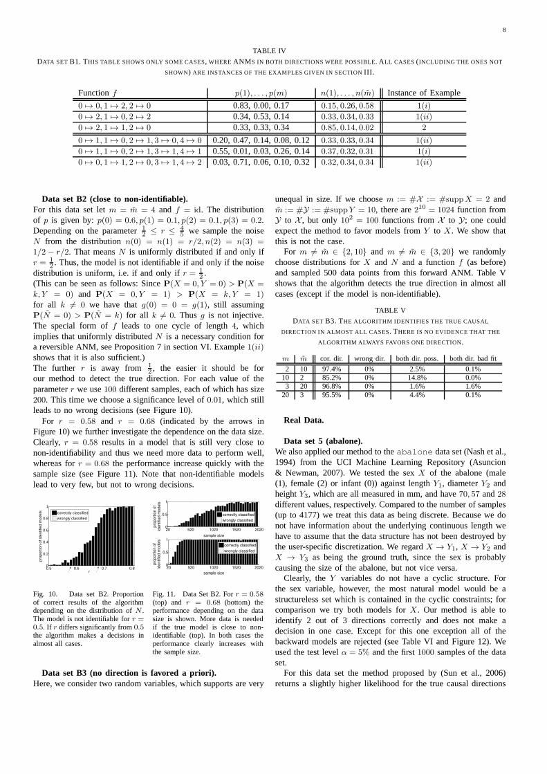
DATA SET B1. THIS TABLE SHOWS ONLY SOME CASES, WHERE ANM S IN BOTH DIRECTIONS WERE POSSIBLE. ALL CASES (INCLUDING THE ONES NOT

SHOWN) ARE INSTANCES OF THE EXAMPLES GIVEN IN SECTIONIII.

Functionf p(1), . . . , p(m) n(1), . . . , n(m) Instance of Example

0 7→ 0, 1 7→ 2, 2 7→ 0 0.83, 0.00, 0.17 0.15, 0.26, 0.58 1(i)

0 7→ 2, 1 7→ 0, 2 7→ 2 0.34, 0.53, 0.14 0.33, 0.34, 0.33 1(ii)

0 7→ 2, 1 7→ 1, 2 7→ 0 0.33, 0.33, 0.34 0.85, 0.14, 0.02 2

0 7→ 1, 1 7→ 0, 2 7→ 1, 3 7→ 0, 4 7→ 0 0.20, 0.47, 0.14, 0.08, 0.12 0.33, 0.33, 0.34 1(ii)

0 7→ 1, 1 7→ 0, 2 7→ 1, 3 7→ 1, 4 7→ 1 0.55, 0.01, 0.03, 0.26, 0.14 0.37, 0.32, 0.31 1(i)

0 7→ 0, 1 7→ 1, 2 7→ 0, 3 7→ 1, 4 7→ 2 0.03, 0.71, 0.06, 0.10, 0.32 0.32, 0.34, 0.34 1(ii)

Data set B2 (close to non-identifiable).For this data set letm = m = 4 and f = id. The distributionof p is given by:p(0) = 0.6, p(1) = 0.1, p(2) = 0.1, p(3) = 0.2.Depending on the parameter12 ≤ r ≤ 4

5 we sample the noiseN from the distributionn(0) = n(1) = r/2, n(2) = n(3) =

1/2− r/2. That meansN is uniformly distributed if and only ifr = 1

2 . Thus, the model is not identifiable if and only if the noisedistribution is uniform, i.e. if and only ifr = 1

2 .(This can be seen as follows: SinceP(X = 0, Y = 0) > P(X =

k, Y = 0) and P(X = 0, Y = 1) > P(X = k, Y = 1)

for all k 6= 0 we have thatg(0) = 0 = g(1), still assumingP(N = 0) > P(N = k) for all k 6= 0. Thus g is not injective.The special form off leads to one cycle of length4, whichimplies that uniformly distributedN is a necessary condition fora reversible ANM, see Proposition 7 in section VI. Example1(ii)

shows that it is also sufficient.)The further r is away from 1

2 , the easier it should be forour method to detect the true direction. For each value of theparameterr we use100 different samples, each of which has size200. This time we choose a significance level of0.01, which stillleads to no wrong decisions (see Figure 10).

For r = 0.58 and r = 0.68 (indicated by the arrows inFigure 10) we further investigate the dependence on the datasize.Clearly, r = 0.58 results in a model that is still very close tonon-identifiability and thus we need more data to perform well,whereas forr = 0.68 the performance increase quickly with thesample size (see Figure 11). Note that non-identifiable modelslead to very few, but not to wrong decisions.

0.5 0.6 0.7 0.80

0.2

0.4

0.6

0.8

1

r

prop

ortio

n of

iden

tifie

d m

odel

s

correctly classified

wrongly classified

Fig. 10. Data set B2. Proportionof correct results of the algorithmdepending on the distribution ofN .The model is not identifiable forr =0.5. If r differs significantly from0.5the algorithm makes a decisions inalmost all cases.

20 520 1020 1520 20200

0.5

1

sample size

pro

po

rtio

n o

fid

en

tifie

d m

od

els

correctly classified

wrongly classified

20 520 1020 1520 20200

0.5

1

sample size

pro

po

rtio

n o

fid

en

tifie

d m

od

els

correctly classified

wrongly classified

Fig. 11. Data Set B2. Forr = 0.58(top) and r = 0.68 (bottom) theperformance depending on the datasize is shown. More data is neededif the true model is close to non-identifiable (top). In both cases theperformance clearly increases withthe sample size.

Data set B3 (no direction is favored a priori).Here, we consider two random variables, which supports are very

unequal in size. If we choosem := #X := #suppX = 2 andm := #Y := #suppY = 10, there are210 = 1024 function fromY to X , but only 102 = 100 functions fromX to Y; one couldexpect the method to favor models fromY to X. We show thatthis is not the case.

For m 6= m ∈ 2, 10 and m 6= m ∈ 3, 20 we randomlychoose distributions forX and N and a functionf (as before)and sampled 500 data points from this forward ANM. Table Vshows that the algorithm detects the true direction in almost allcases (except if the model is non-identifiable).

TABLE V

DATA SET B3. THE ALGORITHM IDENTIFIES THE TRUE CAUSAL

DIRECTION IN ALMOST ALL CASES. THERE IS NO EVIDENCE THAT THE

ALGORITHM ALWAYS FAVORS ONE DIRECTION.

m m cor. dir. wrong dir. both dir. poss. both dir. bad fit

2 10 97.4% 0% 2.5% 0.1%10 2 85.2% 0% 14.8% 0.0%3 20 96.8% 0% 1.6% 1.6%

20 3 95.5% 0% 4.4% 0.1%

Real Data.

Data set 5 (abalone).We also applied our method to theabalone data set (Nash et al.,1994) from the UCI Machine Learning Repository (Asuncion& Newman, 2007). We tested the sexX of the abalone (male(1), female (2) or infant (0)) against lengthY1, diameterY2 andheightY3, which are all measured in mm, and have70, 57 and28different values, respectively. Compared to the number of samples(up to 4177) we treat this data as being discrete. Because we donot have information about the underlying continuous length wehave to assume that the data structure has not been destroyedbythe user-specific discretization. We regardX → Y1, X → Y2 andX → Y3 as being the ground truth, since the sex is probablycausing the size of the abalone, but not vice versa.

Clearly, theY variables do not have a cyclic structure. Forthe sex variable, however, the most natural model would be astructureless set which is contained in the cyclic constraints; forcomparison we try both models forX. Our method is able toidentify 2 out of 3 directions correctly and does not make adecision in one case. Except for this one exception all of thebackward models are rejected (see Table VI and Figure 12). Weused the test levelα = 5% and the first1000 samples of the dataset.

For this data set the method proposed by (Sun et al., 2006)returns a slightly higher likelihood for the true causal directions

9

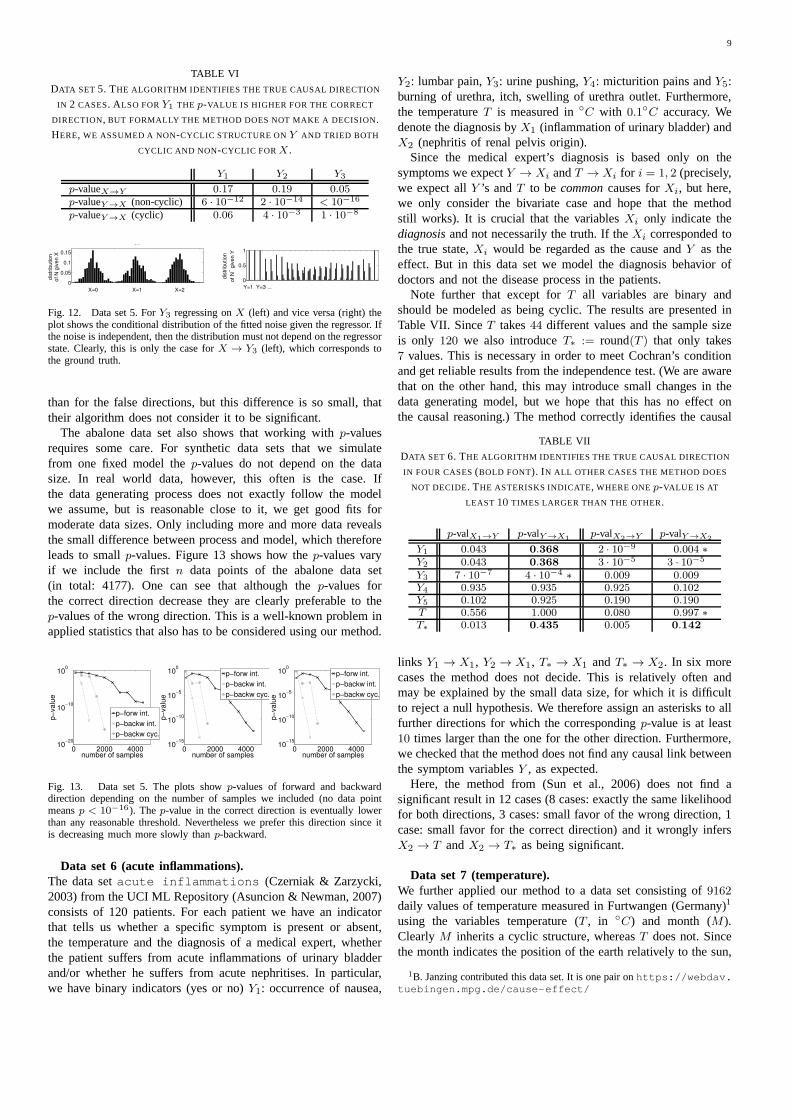
TABLE VI

DATA SET 5. THE ALGORITHM IDENTIFIES THE TRUE CAUSAL DIRECTION

IN 2 CASES. ALSO FORY1 THE p-VALUE IS HIGHER FOR THE CORRECT

DIRECTION, BUT FORMALLY THE METHOD DOES NOT MAKE A DECISION.

HERE, WE ASSUMED A NON-CYCLIC STRUCTURE ONY AND TRIED BOTH

CYCLIC AND NON-CYCLIC FORX .

Y1 Y2 Y3

p-valueX→Y 0.17 0.19 0.05p-valueY →X (non-cyclic) 6 · 10−12 2 · 10−14 < 10−16

p-valueY →X (cyclic) 0.06 4 · 10−3 1 · 10−8

0

0.05

0.1

0.15

X−>Y

X=0 X=1 X=2

dis

trib

ution

of N

giv

en X

0

0.5

1

Y=1 Y=3 ...

dis

trib

ution

of N

~ g

iven Y

Fig. 12. Data set 5. ForY3 regressing onX (left) and vice versa (right) theplot shows the conditional distribution of the fitted noise given the regressor. Ifthe noise is independent, then the distribution must not depend on the regressorstate. Clearly, this is only the case forX → Y3 (left), which corresponds tothe ground truth.

than for the false directions, but this difference is so small, thattheir algorithm does not consider it to be significant.

The abalone data set also shows that working withp-valuesrequires some care. For synthetic data sets that we simulatefrom one fixed model thep-values do not depend on the datasize. In real world data, however, this often is the case. Ifthe data generating process does not exactly follow the modelwe assume, but is reasonable close to it, we get good fits formoderate data sizes. Only including more and more data revealsthe small difference between process and model, which thereforeleads to smallp-values. Figure 13 shows how thep-values varyif we include the firstn data points of the abalone data set(in total: 4177). One can see that although thep-values forthe correct direction decrease they are clearly preferableto thep-values of the wrong direction. This is a well-known probleminapplied statistics that also has to be considered using our method.

0 2000 400010

−20

10−10

100

number of samples

p−

va

lue

p−forw int.

p−backw int.

p−backw cyc.

0 2000 400010

−15

10−10

10−5

100

number of samples

p−

va

lue

p−forw int.

p−backw int.

p−backw cyc.

0 2000 400010

−15

10−10

10−5

100

number of samples

p−

va

lue

p−forw int.

p−backw int.

p−backw cyc.

Fig. 13. Data set 5. The plots showp-values of forward and backwarddirection depending on the number of samples we included (nodata pointmeansp < 10−16). Thep-value in the correct direction is eventually lowerthan any reasonable threshold. Nevertheless we prefer thisdirection since itis decreasing much more slowly thanp-backward.

Data set 6 (acute inflammations).The data setacute inflammations (Czerniak & Zarzycki,2003) from the UCI ML Repository (Asuncion & Newman, 2007)consists of 120 patients. For each patient we have an indicatorthat tells us whether a specific symptom is present or absent,the temperature and the diagnosis of a medical expert, whetherthe patient suffers from acute inflammations of urinary bladderand/or whether he suffers from acute nephritises. In particular,we have binary indicators (yes or no)Y1: occurrence of nausea,

Y2: lumbar pain,Y3: urine pushing,Y4: micturition pains andY5:burning of urethra, itch, swelling of urethra outlet. Furthermore,the temperatureT is measured inC with 0.1C accuracy. Wedenote the diagnosis byX1 (inflammation of urinary bladder) andX2 (nephritis of renal pelvis origin).

Since the medical expert’s diagnosis is based only on thesymptoms we expectY → Xi andT → Xi for i = 1, 2 (precisely,we expect allY ’s andT to becommoncauses forXi, but here,we only consider the bivariate case and hope that the methodstill works). It is crucial that the variablesXi only indicate thediagnosisand not necessarily the truth. If theXi corresponded tothe true state,Xi would be regarded as the cause andY as theeffect. But in this data set we model the diagnosis behavior ofdoctors and not the disease process in the patients.

Note further that except forT all variables are binary andshould be modeled as being cyclic. The results are presentedinTable VII. SinceT takes44 different values and the sample sizeis only 120 we also introduceT∗ := round(T ) that only takes7 values. This is necessary in order to meet Cochran’s conditionand get reliable results from the independence test. (We areawarethat on the other hand, this may introduce small changes in thedata generating model, but we hope that this has no effect onthe causal reasoning.) The method correctly identifies the causal

TABLE VII

DATA SET 6. THE ALGORITHM IDENTIFIES THE TRUE CAUSAL DIRECTION

IN FOUR CASES(BOLD FONT). IN ALL OTHER CASES THE METHOD DOES

NOT DECIDE. THE ASTERISKS INDICATE, WHERE ONEp-VALUE IS AT

LEAST 10 TIMES LARGER THAN THE OTHER.

p-valX1→Y p-valY →X1p-valX2→Y p-valY →X2

Y1 0.043 ∗0.368 ∗ 2 · 10−9 ∗0.004 ∗

Y2 0.043 ∗0.368 ∗ 3 · 10−5 3 · 10−5

Y3 7 · 10−7 ∗4 · 10−4 ∗ 0.009 0.009Y4 0.935 0.935 0.925 0.102Y5 0.102 ∗0.925 ∗ 0.190 0.190T 0.556 ∗1.000 ∗ 0.080 ∗0.997 ∗

T∗ 0.013 ∗0.435 ∗ 0.005 ∗0.142 ∗

links Y1 → X1, Y2 → X1, T∗ → X1 andT∗ → X2. In six morecases the method does not decide. This is relatively often andmay be explained by the small data size, for which it is difficultto reject a null hypothesis. We therefore assign an asterisks to allfurther directions for which the correspondingp-value is at least10 times larger than the one for the other direction. Furthermore,we checked that the method does not find any causal link betweenthe symptom variablesY , as expected.

Here, the method from (Sun et al., 2006) does not find asignificant result in 12 cases (8 cases: exactly the same likelihoodfor both directions, 3 cases: small favor of the wrong direction, 1case: small favor for the correct direction) and it wrongly infersX2 → T andX2 → T∗ as being significant.

Data set 7 (temperature).We further applied our method to a data set consisting of9162

daily values of temperature measured in Furtwangen (Germany)1

using the variables temperature (T , in C) and month (M).ClearlyM inherits a cyclic structure, whereasT does not. Sincethe month indicates the position of the earth relatively to the sun,

1B. Janzing contributed this data set. It is one pair onhttps://webdav.tuebingen.mpg.de/cause-effect/

10

which is causing the temperature on earth, we takeM → T as theground truth. Here, we aggregate states and use months insteadof days. Again, this is done in order to meet Cochran’s condition;it is not a scaling problem of our method (if we do not aggregatethe method returnspdays→T = 0.9327 andpT→days = 1.0000).

For 1000 data points both directions are rejected(p-valueM→T = 3e − 4, p-valueT→M = 1e − 13). Figure14 shows, however, that again thep-valuesM→T are decreasingmuch more slowly thanp-valuesT→M . Using other criteria thansimplep-values we still may prefer this direction and propose itas the true one.

Fig. 14. Data set 7 and Data set 8. Left: The plot showp-values of forwardand backward direction depending on the number of samples weincluded (nodata point meansp < 10−16). Again we prefer the correct direction sincethe p-values are decreasing much more slowly thanp-backward. Right: Thedata set does not allow an ANM in any of the two directions. Therefore themethod does not propose an answer.

The method proposed in (Sun et al., 2006) finds a largerlikelihood for the correct direction, but does not considerthisdifference as being significant.

Data set 8 (faces).This data set (Armann & Bulthoff, 2010) (4499 instances) showsthe limitations of ANMs. Here,X represents a parameter usedto create pictures of artificial faces.X takes values between0and 14, where 0 corresponds to a female face,14 correspondsto a face that is rather masculine. All other parameter valuesare interpolated. These faces were shown to some subjects whohad to indicate whether they believe this is a male (Y = 1) ora female (Y = 0) face. In this example we regardX as beingthe cause ofY . However, the data do not admit an ANM in anydirection (pX→Y = 0 and pY→X = 0). Thus, the method doesnot make a mistake, but does not find the correct answer, either.On this data set the method in (Sun et al., 2006) again detectsan insignificantly larger likelihood for the correct direction.

It is possible, however, to include generalizations of ANMsthat are capable of modeling this data set. One possibility is toconsider models of the form

Y = f(X +N), N ⊥⊥ X and X = g(Y + N), N ⊥⊥ Y (3)

with some possibly non-invertible functionsf and g (for con-tinuous data, a similar model has been proposed by Zhang &Hyvarinen (2009)). In this model the functionf does not only acton the support ofX, but on an enlarged space. Using a methodthat is based on the same ideas described in section IV one is ableto fit this data set quite well (pX→Y = 1.000 and pY→X = 0).However, we do not have any theoretical identifiability results andthe method has one further drawback: Simulations show that itoften prefers the variable with the smaller support as the effect.

In particular, we can indicate why the model class at the righthand side of equation (3) gets too large ifX is a binary variableandY is the discretization of a continuous variable: If one setsg

to be the Heaviside step function defined byg(w) = 1 if w ≥ 0

and g(w) = 0 otherwise, equation (3) leads to (withm(t) theprobability mass function ofM := −N)

P(X = 1|Y = y) = P(y + N ≥ 0) = P(M ≤ y) =

y∑

t=−∞

m(t).

Hence, every conditional for whichP(X = 1|Y = y) ismonotonously increasing can be described by an ANM. But evensome models that we regard as a natural examples forX → Y

lead to such a monotonously increasing conditional: E.g.PY |X=0

andPY |X=1 being discretized Gaussians with equal variance anddifferent means.

VI. PROOFS

A. Proof of Theorem 1

Proof:

⇒: First we assumesupp Y = y0, . . . , ym with y0 < y1 <

. . . < ym. This implies thatNmax := minn ∈ N |P(N =

n) > 0 is finite. Define the non-empty setsCi :=

suppX|Y = yi, for i = 0, . . . ,m. That meansC0, . . . , Cm ⊂

suppX are the smallest sets satisfyingP(X ∈ Ci | Y =

yi) = 1. For all i, j it follows that

Ci = Cj or Ci ∩ Cj = ∅ andf |Ci

= ci = const. (4)

This is proved by an induction argument.Base step: ConsiderCm corresponding to the largestvalue ym = maxf(x) |x ∈ X + Nmax of supp Y .Assuming f(x1) < f(x2) for x1, x2 ∈ Cm leads toym = f(x1) + Nmax < f(x2) + Nmax = ym andtherefore to a contradiction. Induction step: ConsiderCk

and assume properties (4) are satisfied for allCk

withk < k ≤ m. If x ∈ Ck ∩ C

kfor somek

⇒P(N = yk − f(x)) = P(N = yk − f(x)) > 0 ∀x ∈ Ck

⇒ Ck⊂ Ck ⇒ C

k= Ck ⇒ f |

Ck

= f |C

k

= const

Furthermore, if Ck ∩ Ck

= ∅ ∀k < k ≤ m, thenf |

Ck

= const using the same argument as forCm.

Thus we can choose some setsC0, . . . , Cl from C0, . . . , Cm,where l ≤ m, such thatC0, . . . , Cl are disjoint, andck := f(Ck) are pairwise different values. Without loss ofgenerality assumeC0 = C0. Further, even the sets

ck + suppN := ck + h : P(N = h) > 0

are pairwise different: Ifyi = ck + h1 = cl + h2 thenCk ⊂

supp (X|Y = yi) = Ci andCl ⊂ Ci, which impliesk = l.Now consider the case whereY has infinite andX finitesupport:suppX = x0, . . . , xp. Then we defineC0, . . . , Cl

to be disjoint sets, such thatf is constant on each of them:ci := f(Ci). This time, it does not matter which of these setsis calledC0. Again, we will deduce that the setsck+suppN

are disjoint:The setsDi := suppY |X = xi fulfill

Di = Dj or Di ∩ Dj = ∅ andg |Di

= di = const.

Thus we haveck + suppN and ck + suppN are eitherequal or disjoint. But ifck + suppN = cl + suppN for

11

k 6= l it follows for xa ∈ Ck, xb ∈ Cl and ally ∈ ck +

suppN (since there is a backward modelX = g(Y )+N)

P(X = xa, Y = y)

P(X = xb, Y = y)= const

⇒P(X = xa) ·P(N = y − f(xa))

P(X = xb) ·P(N = y − f(xb))= const

⇒P(N = y − f(xa))

P(N = y − f(xb))= const

and thusP(N = 0)/P(N = r) = const,∀r ∈ suppN .This is only possible for a uniformly distributedN ,which leads to a contradiction sinceY has been assumedto have infinite support.

Thus we have proved condition c). For a) it remains to showthat the setsCi are shifted versions of each other. This partof the proof is valid for both cases (eitherX or Y has finitesupport): ConsiderCi for anyi. According to the assumptionthat an ANMY → X holds we have

N |Y = c0d= N |Y = ci

⇔ X − g(c0)|Y = c0d= X − g(ci)|Y = ci

⇒ X + di|Y = c0d= X|Y = ci (∗)

with di = g(ci) − g(c0). Thus Ci = C0 + di (includingd0 = 0), which completes conditions a).To prove b) observe that we have for allx ∈ Ci

P(X = x)

P(X ∈ Ci)=

P(X = x)P(N = ci − f(x))∑

x∈CiP(X = x)P(N = ci − f(x))

=P(X = x,N = ci − f(x))

P(Y = ci)= P(X = x | Y = ci)

(∗)= P(X = x− di |Y = c0)

=P(X = x− di, N = c0 − f(x− di))

P(Y = c0)

=P(X = x− di)

P(X ∈ C0)

⇐: In order to show that we have a reversible ANM, we haveto construct ag, such thatX = g(Y ) + N . Therefore definethe functiong as follows:g(y) = 0,∀y ∈ c0 + suppN andg(y) = di,∀y ∈ ci + suppN, i > 0. (This is well-definedbecause of a) and c).) The noiseN is determined by the jointdistributionP

(X,Y ), of course. It remains to check, whetherthe distribution ofN |Y = y is independent ofy. Considera fixed y and choosei such thaty ∈ ci + suppN . SinceCi = C0 + di the conditiong(y) + h ∈ Ci is satisfied forall h ∈ C0 and therefore independently ofy andci. Now, ifg(y) + h ∈ Ci we have

P(N = h |Y = y) =P(X = g(y) + h, Y = y)

P(Y = y)

=P(X = g(y) + h,N = y − f(g(y) + h))

P(Y = y)

=P(X = g(y) + h)P(N = y − ci)

∑

x∈CiP(X = x)P(N = y − f(x))

=P(X = g(y) + h)

P(X ∈ Ci)=

P(X = g(y) + h− di)

P(X ∈ C0)

=P(X = h)

P(X ∈ C0)

which does not depend ony. And if g(y) + h /∈ Ci thenP(N = h |Y = y) = 0, which does not depend ony either.

B. Proof of Theorem 3

Proof: We distinguish between two different cases:

a) P(N = k) > 0∀m ≤ k ≤ l and P(N = k) = 0 for allotherk.

X

Y

x1 x2x1 x2

w1

f(x1)

f(x2)

w2

Fig. 15. Visualization of the path from equation (5). Here,w2 = f(x2) +Nmax andw1 = f(x1) +Nmax.

⇒: Assume that there is an ANM in both directionsX → Y and Y → X. As mentioned above we havea freedom of choosing an additive constant for theregression function. In the remainder of this proof werequire P(N = k) = P(N = k) = 0∀k < 0 andP(N = 0),P(N = 0) > 0. The largestk, such thatP(N = k) > 0 will be calledNmax. In analogy to theproof above we defineCy := suppX|Y = y for ally ∈ suppY .At first we note that allCy are shifted versions ofeach other (since there is a backward ANM) andadditionally, they are finite sets (otherwise it followsfrom the compact support ofN that there are infinitelymany infinite setsf−1(f(x)) on which f is constant,which contradicts the assumptions.) Start with anyx1that satisfiesx1 = minf−1(f(x1)) and define

x1 := min

x ∈ Cf(x1)+Nmax\ f−1(f(x1))

This impliesf(x1) > f(x1) andx1 ∈ Cf(x1).If such an x1 does not exist because the seton the right hand side is empty, then it can-not exist for any choice ofx1: It is clear thatCf(x1)+Nmax

= f−1(f(x1)) and then we considerthe first Cf(x1)+Nmax+i that is not empty. Thenthis set must bef−1(f(x1)) for some x1. Thisleads to an iterative procedure and to the requireddecomposition ofsuppX.

We have that either

maxf−1(f(x1)) > maxf−1(f(x1)) or

minf−1(f(x1)) < minf−1(f(x1)) :

Otherwise Cf(x1) and Cf(x1)−1 satisfymaxCf(x1)−1 ≥ maxCf(x1) and minCf(x1)−1 ≤

minCf(x1). Because ofx1 ∈ Cf(x1), x1 /∈ Cf(x1)−1

this contradicts the existence of an backward ANM.We therefore assume without loss of generalitymaxf−1(f(x1)) > maxf−1(f(x1)). Then weeven havex1 > x1, x1 = minCf(x1)+Nmax

andx1 = minCf(x1)+Nmax+1. (Otherwise we use the

12

same argument as above withCf(x1)+Nmaxand

Cf(x1)+Nmax+1.) Define further

x2 := min f−1(f(x1) +Nmax + 1)

Sincef−1(f(x1)) ⊂ Cf(x1)+Nmax, but f−1(f(x1)) ∩

Cf(x1)+Nmax+1 = ∅, such a value must exist. Again,we can definex2 in the same way as above.Set y1 := f(x1) + Nmax and z1 := f(x1) + 2 · Nmax

and consider the finite box from(minCy1, y1) to

(maxCz1 , z1). This box contains all the support fromX | Y = f(x1) + Nmax + i, where i = 0, . . . , Nmax.Assume we know the positions in this box, whereP

(X,Y ) is larger than zero. Then this box determinesthe support ofX |Y = f(x1) + 2 · Nmax + 1 (theline above the box) just using the support ofN andN . Iterating gives us the whole support ofP(X,Y ) inthe box above (fromy2 = f(x2) + Nmax to z2 =

f(x2) + 2 · Nmax). Since the width of the boxes arebounded by3 ·maxCf(x1) −minCf(x1), for example,at some point the box ofxn must have the same supportas the one ofx1. Figure 15 shows an example, in whichn = 2. Using only the distributions ofN andN we cannow determine a factorα for which P(X = x1, Y =

f(x1) +Nmax) = α ·P(X = xn, Y = f(xn) +Nmax)

This is done by following a sequence between(x1, y1)

and (xn, yn) using only horizontal and vertical steps:

(x1, y1), (x1, y1), (x1, f(x2)), (x2, f(x2)),

(x2, y2), (x2, y2), . . . , (xn, yn) (5)

(cf Figure 15). Since this factor only depends on thedistributions ofN andN , the sameα satisfiesP(X =

xn, Y = f(xn) + Nmax) = α · P(X = x2n−1, Y =

f(x2n−1) +Nmax) and therefore

P(X = x1, Y = f(x1) +Nmax) = αk·

P(X = x(k+1)n−k, Y = f(x(k+1)n−k) +Nmax)

Note that a corresponding equation with the sameconstantα holds for the direction to the left ofx1. Thisleads to a contradiction, since there is no probabilitydistribution forX with infinite support that can fulfillthis condition (no matter ifα is greater, equal or smallerthan1).

⇐: This direction is proved in exactly the same way as inTheorem 1.

b) P(N = k) > 0 ∀ k ∈ Z.SinceX and Y are dependent there arey1 and y2, suchthat g(y1) 6= g(y2) with g being the “backward func-tion”. Comparing P(X = k, Y = y1), k ≥ m andP(X = k, Y = y2), k ≥ m we can identify thedifferenced := g(y2) − g(y1). Wlog considerd > 0. Weuse P(X=m−1,Y=y1)

P(X=m,Y=y1)=

P(X=m+d−1,Y=y2)P(X=m+d,Y=y2)

in order todetermineP(X = m− 1, Y = y1) and thenP(X = m− 1)

(usingf andPN ). Iterations lead to allP(X = x).

C. Proof of Theorem 4

Each distributionY |X = xj has to have the same support (upto an additive shift) and thus the same number of elements with

probability larger than0: #suppX · #suppN = k · #suppY .This proofs (i). For (ii) we now consider 3 different cases: 1. fandg are bijective, 2.g is not injective and 3.f is not injective.These three cases are sufficient sincef and g injective impliesn = m and f and g bijective. For each of those cases we showthat a necessary condition for reversibility includes at least oneadditional equality constraint forPX or PN .

1st case:f andg are bijective.Proposition 6: Assume Y = f(X) + N, N ⊥⊥ X forbijective f and n(l) 6= 0, p(k) 6= 0 ∀k, l. If the model isreversible with a bijectiveg, thenX andY are uniformlydistributed.

Proof: Since g is bijective we have that∀y∃ty :

g(ty) = g(y)− 1. From (2) we can deduce

n(

y − f(x+ 1))

p(x+ 1)

n(

ty − f(x))

p(x)=

n(

x+ 1− g(y))

q(y)

n(

x+ 1− g(y))

q(ty)

which implies

p(x+ 1)

p(x)=

n(

ty − f(x))

q(y)

n(

y − f(x+ 1))

q(ty)and

1 =p(x+m)

p(x)=

∏m−1k=0 n

(

ty − f(x+ k))

q(y)m

∏m−1k=0 n

(

y − f(x+ k + 1))

q(ty)m

Sincef is bijective it follows thatq(y) = q(ty). This holdsfor all y and thusY andX are uniformly distributed.

2nd case:g is not injective.Assume g(y0) = g(y1). From (2) it follows thatn(

y0−f(x))

n(

y1−f(x)) =

q(y0)q(y1)

∀x and thusn(

y0−f(x))

n(

y1−f(x)) =

n(

y0−f(x))

n(

y1−f(x)) ∀x, x, which imply equality constraints onn.

To determine the number of constraints we define a functionthat maps the arguments of the numerator to those of thedenominator

hy0,y1,f :Im(y0 − f) → Z/mZ

y0 − f(x) 7→ y1 − f(x).

We sayh has a cycle if there is az ∈ N, s.t. hk(a) =

(h . . . h)(a) ∈ Im(y0 − f) ∀k ≤ z and hz(a) = a. For

example:2 h7→ 4

h7→ 6

h7→ 0

h7→ 2.

Proposition 7: AssumeY = f(X) + N, N ⊥⊥ X andn(l) 6= 0, p(k) 6= 0 ∀k, l. Assume further that the modelis reversible with a non-injectiveg.

• If h has at least one cycle,#Imf − #cycles+ 1

parameters ofn are determined by the others.• If h has no cycles,#Imf parameters ofn are deter-

mined by the others.Proof: Assume h has a cycle of length

r: n1h7→ n2

h7→ . . .

h7→ nr

h7→ n1 (here,

y0 − n1, . . . , y0 − nr ∈ Imf), then q(y0)q(y1)

= 1 becauseq(y0)

r

q(y1)r=

n(n1)n(n2)

· n(n2)n(n3)

. . .n(nr)n(n1)

=n(n1)n(n1)

= 1

and n(

y0 − f(x))

= n(

y1 − f(x))

∀x, that isn(n1) = n(n2) = . . . = n(nr). Thus we getr − 1 equalityconstraints for each cycle of lengthr. For any (additional)non-cyclic structure of lengthr: n1 7→ n2 7→ . . . 7→ nr andnr /∈ Im(y0 − f) (here,y0 − n1, . . . , y0 − nr−1 ∈ Imf),we haven(n1) = . . . = n(nr) and thusr − 1 equalityconstraints. Together with the normalization these are

13

#Imf −#cycles+ 1 constraints.

If h has no cycle, we have#Imf−1 independent equationsplus the sum constraint. E.g.:n(2)

n(4)=

n(4)n(6)

=n(3)n(5)

implies

n(4) = n(6)n(3)n(5)

and n(2) =n(4)2

n(6). Further,

n(

y0 − f(x))

n(

y1 − f(x)) =

q(y0)

q(y1)=

∑

x p(x)n(y0 − f(x)∑

x p(x)n(y1 − f(x))

introduces a functional relationship betweenp andn.Note that if m does not have any divisors, there are nocycles and thus#Imf parameters ofn are determined. Wehave the following corollaryCorollary 8: In all cases the number of fixed parameters islower bounded by⌈1/2 ·#Imf⌉ + 1 ≥ 2 .

3rd case:f is not injective.Assumef(x0) = f(x1). In a slight abuse of notation wewrite

g − g :Z/mZ× Z/mZ → Z/mZ

(y, y) 7→ g(y)− g(y).

Similar as above, we define

hx0,x1,g :Im

(

x0 − (g − g))

→ Z/mZ

x0 − g(y) + g(y) 7→ x1 − g(y) + g(y).

We say thath has a cycle if there is az ∈ N, s.t.hk(a) =(h . . . h)(a) ∈ Im

(

x0 − (g − g))

∀k ≤ z andhz(a) = a.Proposition 9: AssumeY = f(X) +N, N ⊥⊥ X, f is notinjective andn(l) 6= 0, p(k) 6= 0 ∀k, l. Assume further thatthe model is reversible for a functiong.

• If h has at least one cycle,#Im(g − g)−#cycles+ 1

parameters ofp are determined by the others.• If h has no cycles,#Im(g − g) parameters ofp are

determined by the others.

Proof: From (2) it follows thatp(x0)p(x1)

=n(

x0−g(y))

n(

x1−g(y)) =

p(

x0−g(y)+g(y))

·n

(

y−f(

x0−g(y)+g(y))

)

p(

x1−g(y)+g(y))

·n

(

y−f(

x1−g(y)+g(y))

) ∀y, y. The rest

follows analogously to the proof of Proposition 7.If (x1−x0) does not dividem, there are no cycles and thus#Im(g − g) parameters ofp are determined.Corollary 10: In all cases the number of fixed parametersis lower bounded by⌈1/2 ·#Im(g − g)⌉+ 1 ≥ 2 .

Remark 2:Note that some of the constraints described abovedepend on the backward functiong. This introduces no problemsbecause of the following reason: If we put any (prior) measureon the set of all possible parametersp(0), p(1), . . . , p(n− 1) (oron n(0), . . . , n(m− 1)) that is absolutely continuous with respectto the Lebesgue measure, a single equality constraint reduces theset of possible parameters to a set of measure zero. There areonly finitely many possibilities to choose the functiong and thuseven the union of all those parameter sets has measure zero.

VII. C ONCLUSIONS ANDFUTURE WORK

We proposed a method that tries to infer the cause-effect rela-tionship between two discrete random variables using the conceptof ANMs. We proved that for generic choices the direction ofa discrete ANM is identifiable in the population case and wedeveloped an efficient algorithm that is able to apply the proposed

inference principle to a finite amount of data from two variables;we also mentioned the limitations ofp-values on real world datasets with changing data size.

Since it is known thatχ2 fails for small data sizes, changingthe independence test for those cases may lead to an evenhigher performance of the algorithm. Further, our method canbe generalized in different directions: (1) handling more thantwo variables is straightforward from a practical point of view,although one may have to introduce regularization to make theregression computationally feasible. Therefor, the work by Mooijet al. (2009) and the practical approach of combining constraint-based methods and ANMs by Tillman et al. (2009) may behelpful. (2) One should work on practically feasible extensionsof ANMs and (3) it should be investigated how our procedurecan be applied to the case, where one variable is discrete andtheother continuous. Corresponding identifiability results remain tobe shown. (4) We further believe that it is valuable to test thefollowing principle for causal inference: One decides forX → Y

not only if one finds an ANM in this direction and not the other,but also if the observed empirical distribution isreasonably closerto the set of distributions that allow for an ANM fromX to Y

than to the set of distributions that allow for an ANM fromYto X (e.g. the KL divergence to the subset ANMX→Y is smallerthan to the subset ANMY →X , see section III-C). Clearly, thechallenges of computing the distances to those sets of distributionsand quantifying whatreasonablycloser means have to be solved.

We answered the theoretical question of identifiability, but infuture work the concept of ANMs (like any proposed conceptof causal inference) has to be addressed empirically: It shouldbe tested on a large number of real world data sets, for whichthe ground truth is known. Our small collection of experiments,for example, only give a hint that ANMs may help for causalinference. It is still possible that exhaustive experiments show thatthe assumptions current methods for causal inference are basedon are most often not met in nature. Nevertheless we regard ourwork as promising and hope that more fundamental and generalprinciples for identifying causal relationships will be developedthat cover ANMs as a special case.

ACKNOWLEDGEMENT

The authors want to thank Fabian Gieringer for collaborating onsection III-C and Joris Mooij, Kun Zhang and Stefan Harmelingfor helpful comments.

REFERENCES

Agresti, A. (2002). Categorical Data Analysis. Wiley Series inProbability and Statistics. Wiley-Interscience, 2nd ed.,2002.

Armann, R., & Bulthoff, I. (2010). in preparation.https://webdav.tuebingen.mpg.de/cause-effect/.

Asuncion, A., & Newman, D. (2007). UCI machine learningrepository.http://archive.ics.uci.edu/ml/.

Cochran, W. G. (1954). Some methods for strengthening thecommonχ2 tests.Biometrics, 10:417–451, 1954.

Czerniak, J., & Zarzycki, H. (2003). Application of rough setsin the presumptive diagnosis of urinary system diseases. InArtifical Inteligence and Security in Computing Systems, 9th In-ternational Conference Proceedings, 41–51. Kluwer AcademicPublishers.

Heckerman, D., Meek, C., & Cooper, G. (1999). A Bayesian ap-proach to causal discovery. In C. Glymour, & G. Cooper, eds.,

14

Computation, Causation, and Discovery, 141–165. Cambridge,MA: MIT Press.

Hoyer, P., Janzing, D., Mooij, J., Peters, J., & Scholkopf,B.(2009). Nonlinear causal discovery with additive noise models.In Advances in Neural Information Processing Systems (NIPS),689–696. Vancouver, Canada: MIT Press.

Janzing, D., Peters, J., Mooij, J. M., & Scholkopf, B. (2009).Identifying confounders using additive noise models. InPro-ceedings of the 25th Conference on Uncertainty in ArtificialIntelligence (UAI), 249–257. Corvallis, Oregon: AUAI Press.

Janzing, D., & Steudel, B. (2010). Justifying additive-noise-modelbased causal discovery via algorithmic information theory.Open Systems and Information Dynamics, 17, 189–212.

Kano, Y., & Shimizu, S. (2003). Causal inference using non-normality. In Proceedings of the International Symposium onScience of Modeling, the 30th Anniversary of the InformationCriterion, 261–270. Tokyo, Japan.

Mooij, J., Janzing, D., Peters, J., & Scholkopf, B. (2009).Regres-sion by dependence minimization and its application to causalinference. InProceedings of the 26th International Conferenceon Machine Learning (ICML), 745–752. Montreal: Omnipress.

Nash, W., Sellers, T., Talbot, S., Cawthorn, A., & Ford, W.(1994). The Population Biology of Abalone (Haliotis species)in Tasmania. I. Blacklip Abalone (H. rubra) from the NorthCoast and Islands of Bass Strait. Sea Fisheries Division,Technical Report No. 48 (ISSN 1034-3288).

Pearl, J. (2000). Causality: Models, reasoning, and inference.Cambridge University Press.

Peters, J., Janzing, D., Gretton, A., & Scholkopf, B. (2009).Detecting the direction of causal time series. InProceedingsof the 26th International Conference on Machine Learning(ICML), 801–808. Montreal: Omnipress.

Peters, J., Janzing, D., & Scholkopf, B. (2010). Identifying Causeand Effect on Discrete Data using Additive Noise Models. InProceedings of the 13th International Conference on ArtificialIntelligence and Statistics (AISTATS), vol. 9, 597–604.

Shimizu, S., Hoyer, P. O., Hyvarinen, A., & Kerminen, A. J.(2006). A linear non-Gaussian acyclic model for causaldiscovery. Journal of Machine Learning Research, 7, 2003–2030.

Spirtes, P., Glymour, C., & Scheines, R. (1993).Causation,prediction, and search. Springer-Verlag. (2nd edition MIT Press2000).

Sun, X., Janzing, D., & Scholkopf, B. (2006). Causal inferenceby choosing graphs with most plausible Markov kernels. InProceedings of the 9th International Symposium on ArtificialIntelligence and Mathematics, 1–11. Fort Lauderdale, FL.

Sun, X., Janzing, D., & Scholkopf, B. (2008). Causal reasoning byevaluating the complexity of conditional densities with kernelmethods.Neurocomputing, 71, 1248–1256.

Tillman, R., Gretton, A. & Spirtes, P. (2009). Nonlinear directedacyclic structure learning with weakly additive noise models.In Advances in Neural Information Processing Systems (NIPS),Vancouver, Canada, December 2009.

Verma, T. & Pearl, J. (1991) Equivalence and synthesis of causalmodels. InProceedings of the 6th Conference on Uncertaintyin Artificial Intelligence (UAI), pages 255–270, New York, NY,USA, 1991. Elsevier Science Inc.

Zhang, K., & Hyvarinen, A. (2009). On the identifiability ofthe post-nonlinear causal model. InProceedings of the 25th

Conference on Uncertainty in Artificial Intelligence (UAI),647–655. Corvallis, Oregon: AUAI Press.

Jonas Petersstudied Mathematics and received aMaster of Advanced Study and the UNWIN prizefrom Cambridge University (UK) in 2007 and aDiplom from the University of Heidelberg (Ger-many) in 2009. He wrote his diploma thesis aboutdetermining the direction of time series based oncausality. For his PhD he is now working on causalinference problems at the Max Planck Institute forBiological Cybernetics in Tubingen. His studieswere supported by the German National AcademicFoundation, the DAAD and the Kurt-Hahn-Trust.

Dominik Janzing received a Diplom in Physicsin 1995 and a PhD in Mathematics in 1998 fromthe University of Tubingen. From 1998-2006 hewas a postdoc and senior scientist at the ComputerScience department of the University of Karlsruhe(TH). Since 2007 he has been working as a seniorscientist at the Max Planck Institute for BiologicalCybernetics. There, he works on causal reasoningfrom statistical data. His approach uses complexityof conditional probability distributions. This idea isstrongly influenced by his previous work on com-

plexity of physical processes and the thermodynamics of information flow.

Bernhard Scholkopf received a doctorate in com-puter science from the Technical University Berlin.His thesis on Support Vector Learning won theannual dissertation prize of the German Associationfor Computer Science (GI). He has researched atAT&T Bell Labs, at GMD FIRST, Berlin, at theAustralian National University, Canberra, and at Mi-crosoft Research Cambridge (UK). In July 2001, hewas appointed scientific member of the Max PlanckSociety. In 2006, he received the J. K. AggarwalPrize of the International Association for Pattern

Recognition. The ISI lists him as a highly cited researcher,and he is a boardmember of the NIPS foundation and of the International Machine LearningSociety.