school of engineering and information tehcnology...figure 33 triple effect evaporator model in acm...
TRANSCRIPT
School of Engineering and Information Tehcnology
Modelling and Optimising Single and
Multiple Effect Evaporators By Using
Aspen Custom Modeler (ACM),
Microsoft Excel and Matlab.
Irfan Affiq Idham Jihadi
A report submitted to the School of Engineering and Information Technology, Murdoch University in partial fulfilment of the requirements for the degree of Bachelor of Engineering Honours
Thesis Supervisor : Dr. Linh Vu
Date : 19/01/2018

Declaration
I, Irfan Affiq Idham Jihadi, declare that this thesis is my own work except for the idea of the
project which is referenced and this document is submitted to School of Engineering and
Information Technology in order to fulfill the requirements of the undergraduate course at
Murdoch University. Also, this document has not been submitted to any other school or academic
institution.
Date:
Irfan Affiq Idham Jihadi

iii
ABSTRACT
The modelling, optimisation and control analyses of single and multiple effect evaporators using
Aspen Custom Modeller (ACM) is carried out to develop programs in different software packages
for both single and multiple effect evaporators from an example of double effect evaporator
model equations written in ACM. To develop the programs, the developed model equations must
be understood thoroughly.
The case study was taken from the example provided by ACM, which was part of the ASPEN
software package. The example from ACM involves double effect evaporators and the procedure
to concentrate glycol from a dilute aqueous solution of 3.5w% of a glycol. A simulation for both
single and multiple effect evaporators is performed by using Microsoft Excel, Matlab and ACM.
Both models perform a steady-state and optimisation simulation. To build the simulation, a study
on the process model is necessarily required. The study will be carried out by using Microsoft
Excel spreadsheet. Microsoft Excel is chosen to be the medium of study because the sequences of
equations solved during performing the simulation is much easy to understand. The simulation
will start with developing the steady-state model for a single effect evaporator. Once the single
effect is tested, then the steady-state model for multiple effects is developed and tested. After
that, the case study is continued with the phase of developing an optimisation simulation of a
single effect evaporator. Subsequently, the optimisation of single effect evaporator is successfully
tested, the case study continues with developing an optimisation for multiple effect evaporators.
The final phase is carried out to run a performance analysis between ‘FSolve’ function and ACM.
Besides performance analysis, a sensitive analysis in both single and multiple effect evaporators is
also being done by using ACM. The performance analysis proves the optimisation simulation in
‘FSolve’ has not much different from the optimisation simulation perform in the ACM and the
sensitive analysis produce an expected result. With the performance and sensitive analysis
results, the case study can conclude that the three software packages successfully simulated
single and multiple effect evaporators. However, there is a plenty of room to make improvements
in this case study.

iv
Acknowledgement
I would like to use this opportunity to express my sincere thanks to Dr. Linh Vu, my thesis
supervisor, for sharing expertise, and sincere and valuable guidance and encouragement
extended to me. I consider myself fortunate to have the opportunity to work with her as she is
entirely dedicated to give advice and opinion in preparing this report as well in the thesis
presentation and pushing me further to give my best in this thesis. Not to forget, I would also like
to thank Professor Parisa Arabzadeh Bahri and Dr. Gareth Lee, the unit coordinators of ENG470
for all the reminders and supports you have given.
I also thank my parents for the encouragement, support and attention. Lastly, I also place on
record, my sense of gratitude to one and all, who directly or indirectly, have lent their hand in this
venture.
v
Table of Content
Contents Declaration ......................................................................................................................................... 0
ABSTRACT .......................................................................................................................................... iii
Acknowledgement ............................................................................................................................ iv
Table of Content ................................................................................................................................. v
List of Figures ................................................................................................................................... vii
List of Tables ...................................................................................................................................... ix
Abbreviations ..................................................................................................................................... x
1.0 Introduction ........................................................................................................................... 1
2.0 Literature Review ................................................................................................................... 3
2.1 Types of Evaporators .......................................................................................................... 4
2.2 Ethylene Glycol Manufacturing Process ............................................................................. 9
2.3 Propylene Glycol Manufacturing Process ........................................................................ 11
2.4 Aspen Custom Modeler (ACM) ........................................................................................ 12
2.5 Matlab (Matrix Laboratory) .............................................................................................. 12
2.6 Microsoft Excel ................................................................................................................. 13
2.7 Sequential Modular Operation ........................................................................................ 13
3.0 Project Objective and Scope ................................................................................................ 14
4.0 Case Study Description and Model Development ............................................................... 15
4.1 Single Effect Evaporator ................................................................................................... 15
4.2 Multi Effect Evaporator .................................................................................................... 17
4.3 Optimisation ..................................................................................................................... 18
5.0 Research Methodology ........................................................................................................ 18
5.1 Development and Testing the Model Equations.............................................................. 20
5.1.1 Collecting and Interpreting Data .............................................................................. 20
5.1.2 Investigation of Double Effect Evaporator Example in Aspen Custom Modeler
(ACM) .................................................................................................................................. 22
vi
5.1.3 Investigation of Steady-state Model in Microsoft Excel Spreadsheet ..................... 24
5.1.4 Investigation of Steady-state Model in Matlab ........................................................ 27
5.1.5 Investigation of Optimisation Model in ACM ........................................................... 28
5.1.6 Investigation of FSolve Model in Matlab ................................................................. 30
5.2 Tabulating and Data Comparison ..................................................................................... 33
6.0 Results .................................................................................................................................. 35
6.1 Steady-state Simulation ................................................................................................... 36
6.1.1 Single Effect Evaporator Steady-state Model .......................................................... 36
6.1.2 Double Effect Evaporator Steady-state Model ........................................................ 39
6.1.3 Triple Effect Evaporator Steady-state Model ........................................................... 41
6.2 Optimisation Simulation ................................................................................................... 47
6.2.1 Single Effect Evaporator Optimisation Model .......................................................... 47
6.2.2 Double Effect Evaporator Optimisation Model ........................................................ 49
6.2.3 Triple Effect Evaporator Optimisation Model .......................................................... 51
6.3 Performance Run and Sensitive Analysis ......................................................................... 55
6.3.1 Performance Comparison between ACM Optimisation and ‘FSolve’ with Costing
Constraint ................................................................................................................................. 55
6.3.2 Sensitive Analysis of the Single and Triple effect evaporator system. ............................ 56
7.0 Conclusion ............................................................................................................................ 60
7.1 Future work ...................................................................................................................... 62
Reference ......................................................................................................................................... 63
Appendix A (Steady-state Result from ACM in Microsoft Excel) ..................................................... 64
Appendix B (Result Comparison) ...................................................................................................... 70
Appendix C (Microsoft Excel Model) ................................................................................................ 73
Appendix D (ACM equations) ........................................................................................................... 78
Appendix E (Step to change decision variables in ACM) .................................................................. 81
Appendix F (Matlab Script) ............................................................................................................... 82

vii
List of Figures
Figure 1 Batch Pan Evaporator (APV 2008) ........................................................................................ 5
Figure 2 Natural Circulation Evaporator (APV 2008) ......................................................................... 5
Figure 3 Rising Film Tubular (APV 2008) ............................................................................................ 6
Figure 4 Falling film tubular (APV 2008) ............................................................................................. 7
Figure 5 Force Circulation Evaporator (APV 2008) ............................................................................. 7
Figure 6 Rising/falling Film Plate evaporator design (APV 2008) ....................................................... 8
Figure 7 Patented feed distribution system (APV 2008) .................................................................... 9
Figure 8 Commercial ethylene oxide hydration plant (Jr 1984) ....................................................... 10
Figure 9 Propylene Glycol Process Plant (Patel 2009) ...................................................................... 11
Figure 10 Flow diagram of single effect evaporator ........................................................................ 15
Figure 11 Flow diagram of double effect evaporator (Ramli 2016) ................................................. 17
Figure 12 Flowchart of the method taken place in the research ..................................................... 19
Figure 13 Collection of data from double effect of evaporator in ACM .......................................... 20
Figure 14 Set of equations in evaporator model ............................................................................. 23
Figure 15 Data flow for steady-state simulation in Microsoft Excel ................................................ 25
Figure 16 Testing sheet for double effect evaporator ..................................................................... 26
Figure 17 Steady-state simulation spreadsheet for double effect evaporator in Microsoft Excel .. 27
Figure 18 Equation is applied for steady-state simulation in the Microsoft Excel ........................... 27
Figure 19 Steady-state simulation in Matlab ................................................................................... 28
Figure 20 Optimisation equations for double evaporators.............................................................. 29
Figure 21 Three variables that manipulated for optimisation test run ........................................... 29
Figure 22 Solver Matlab file for 'FSolve' simulation or the ‘solver’ file ........................................... 31
Figure 23 The ten variables and six objective functions used in the ‘main’ file .............................. 32
Figure 24 Costing equation applied in the 'main' file....................................................................... 33
Figure 25 Method of tabulating result of each simulation for triple effect evaporator system ...... 34
Figure 26 Flow of simulation test in every software ........................................................................ 35
Figure 27 Single evaporator plant model in ACM ............................................................................ 37
Figure 28 Single effect evaporator simulation data from ACM ....................................................... 37
Figure 29 Result for steady-state simulation of single effect evaporator ........................................ 38
Figure 30 Steady-state 'FSolve' simulation result comparison for single effect evaporator ........... 39
Figure 31 Table of result of each simulation for double effect evaporator ..................................... 40
Figure 32 Double effect evaporator ‘FSolve' steady-state simulation result in comparison for
different software packages ............................................................................................................ 41
viii
Figure 33 Triple effect evaporator model in ACM ........................................................................... 41
Figure 34 Triple effect evaporator 'testing sheet' in Microsoft Excel model ................................... 43
Figure 35 Triple effect evaporator model in Matlab ........................................................................ 44
Figure 36 Triple effect evaporator steady-state simulation result in every software ..................... 45
Figure 37 Triple effect evaporator ‘FSolve' steady-state simulation result in comparison for
different software packages ............................................................................................................ 46
Figure 38 Single effect evaporator optimisation costing equations ................................................ 48
Figure 39 Optimisation simulation result in ACM for single effect evaporator plant ...................... 48
Figure 40 'FSolve' with costing equations simulation result for single effect evaporator ............... 49
Figure 41 Optimisation simulation result in ACM for double effect evaporator ............................. 50
Figure 42 'FSolve' with costing equations simulation result for double effect evaporator ............. 51
Figure 43 Triple effect evaporator optimisation costing equations ................................................ 52
Figure 44 Optimisation simulation result in ACM for triple effect evaporator ................................ 52
Figure 45 'FSolve' with costing equations simulation result for triple effect evaporator ............... 54
Figure 46 Optimisation objective function comparison of ACM and 'FSolve' .................................. 55
Figure 47 Mass flowrate of steam vs glycol concentration in final product .................................... 58
Figure 48 Mass Flowrates of final solution vs mass flowrates of steam .......................................... 58
Figure 49 Optimisation Window ...................................................................................................... 81
Figure 50 Steady-state Constraint ta ................................................................................................ 81

ix
List of Tables
Table 1 Evaporation versus Distillation Process(Pabasara 2017)....................................................... 4
Table 2 Fixed process value from the example in ACM ................................................................... 21
Table 3 First test performance analysis result ................................................................................. 56
Table 4 Second test performance analysis result ............................................................................ 59

x
Abbreviations
Greek letters
Abbreviations Description
∆𝑃𝑃 Pressure difference
∆𝑇𝑇 Temperature difference
λ Latent heat
Model Subscript
Abbreviations Description
Atf Heat transfer area
chest Chest
eva Evaporator
g Glycol
𝐻𝐻� Enthalpy
Htf Heat transfer coefficient
i In
𝐾𝐾𝑙𝑙𝑙𝑙 Liquid valve coefficient
𝐾𝐾𝑠𝑠𝑙𝑙 Steam valve coefficient
𝐾𝐾𝑙𝑙𝑙𝑙𝑣𝑣 Vapour valve coefficient
l Liquid
𝑚𝑚 Mass
o out
𝑃𝑃 Pressure
pmp Pump
st Steam
𝑇𝑇 Temperature
vp Vapour
w Water
𝑋𝑋 Concentration

xi
Steam Flow Subscript
Abbreviations Description
𝐻𝐻�𝑠𝑠𝑠𝑠𝑠𝑠 Steam enthalpy into Evaporator 1
𝐻𝐻�𝑠𝑠𝑠𝑠𝑠𝑠2 Steam enthalpy into Evaporator 2
𝐻𝐻�𝑠𝑠𝑠𝑠𝑠𝑠3 Steam enthalpy into Evaporator 3
𝐻𝐻�𝑙𝑙𝑣𝑣𝑜𝑜 Vapour enthalpy out from Evaporator 1
𝐻𝐻�𝑙𝑙𝑣𝑣2𝑜𝑜 Vapour enthalpy out from Evaporator 2
𝐻𝐻�𝑙𝑙𝑣𝑣3𝑜𝑜 Vapour enthalpy out from Evaporator 3
𝑚𝑚𝑠𝑠𝑠𝑠 Mass of steam from feeder to Evaporator 1
𝑚𝑚𝑠𝑠𝑠𝑠2 Mass of steam from Evaporator 1 to Evaporator 2
𝑚𝑚𝑠𝑠𝑠𝑠3 Mass of steam from Evaporator 2 to Evaporator 3
𝑚𝑚𝑙𝑙𝑣𝑣 Mass of vapor produce from Evaporator 1
𝑚𝑚𝑙𝑙𝑣𝑣2 Mass of vapor produce from Evaporator 2
𝑚𝑚𝑙𝑙𝑣𝑣3 Mass of vapor produce from Evaporator 3
𝑃𝑃𝑠𝑠𝑠𝑠𝑠𝑠_𝐸𝐸𝐸𝐸 Pressure steam into Evaporator 1
𝑃𝑃𝑠𝑠𝑠𝑠𝑠𝑠_𝐸𝐸𝐸𝐸2 Pressure steam into Evaporator 2
𝑃𝑃𝑠𝑠𝑠𝑠𝑠𝑠_𝐸𝐸𝐸𝐸3 Pressure steam into Evaporator 3
𝑃𝑃𝑠𝑠𝑠𝑠_𝐹𝐹 Pressure steam from steamer
𝑃𝑃𝑠𝑠𝑠𝑠𝑠𝑠_𝑆𝑆𝐸𝐸 Pressure steam into Steam Valve
𝑃𝑃𝑠𝑠𝑠𝑠𝑠𝑠_𝑆𝑆𝐸𝐸 Pressure steam out of Steam Valve
𝑃𝑃𝑙𝑙𝑣𝑣_𝐸𝐸𝐸𝐸 Pressure steam out from Evaporator 1
𝑃𝑃𝑙𝑙𝑣𝑣_𝐸𝐸𝐸𝐸2 Pressure steam out from Evaporator 2
𝑃𝑃𝑙𝑙𝑣𝑣_𝐸𝐸𝐸𝐸3 Pressure steam out from Evaporator 3
𝑇𝑇𝑠𝑠𝑠𝑠𝑠𝑠_𝐸𝐸𝐸𝐸 Temperature steam into Evaporator 1
𝑇𝑇𝑠𝑠𝑠𝑠𝑠𝑠_𝐸𝐸𝐸𝐸2 Temperature steam into Evaporator 2
𝑇𝑇𝑠𝑠𝑠𝑠𝑠𝑠_𝐸𝐸𝐸𝐸3 Temperature steam into Evaporator 3
𝑇𝑇𝑠𝑠𝑠𝑠_𝑆𝑆𝑆𝑆 Temperature steam from steamer
𝑇𝑇𝑠𝑠𝑠𝑠𝑠𝑠_𝑆𝑆𝐸𝐸 Temperature steam into Steam Valve
𝑇𝑇𝑠𝑠𝑠𝑠𝑠𝑠_𝑆𝑆𝐸𝐸 Temperature steam out from Steam Valve
𝑇𝑇𝑙𝑙𝑣𝑣_𝐸𝐸𝐸𝐸 Temperature steam out from Evaporator 1
𝑇𝑇𝑙𝑙𝑣𝑣_𝐸𝐸𝐸𝐸2 Temperature steam out from Evaporator 2
𝑇𝑇𝑙𝑙𝑣𝑣_𝐸𝐸𝐸𝐸3 Temperature steam out from Evaporator 3

xii
Liquid Flow Subscripts
Abbreviations Description
𝐻𝐻𝑙𝑙𝑠𝑠_𝐸𝐸𝐸𝐸/𝐻𝐻𝑙𝑙𝑠𝑠_𝐸𝐸𝐸𝐸 Enthalpy of liquid in/out of Evaporator 1
𝐻𝐻𝑙𝑙𝑠𝑠_𝐸𝐸𝐸𝐸2/𝐻𝐻𝑙𝑙𝑠𝑠_𝐸𝐸𝐸𝐸2 Enthalpy of liquid in/out of Evaporator 2
𝐻𝐻𝑙𝑙𝑠𝑠_𝐸𝐸𝐸𝐸3/𝐻𝐻𝑙𝑙𝑠𝑠_𝐸𝐸𝐸𝐸3 Enthalpy of liquid in/out of Evaporator 3
𝐻𝐻𝑙𝑙𝑠𝑠_𝐹𝐹𝐹𝐹/𝐻𝐻𝑙𝑙𝑠𝑠_𝐹𝐹𝐹𝐹 Enthalpy of liquid in/out of feed pump in Evaporator 1
𝐻𝐻𝑙𝑙𝑠𝑠_𝐹𝐹𝐹𝐹2/𝐻𝐻𝑙𝑙𝑠𝑠_𝐹𝐹𝐹𝐹2 Enthalpy of liquid in/out of feed pump in Evaporator 2
𝐻𝐻𝑙𝑙𝑠𝑠_𝐹𝐹𝐹𝐹3/𝐻𝐻𝑙𝑙𝑠𝑠_𝐹𝐹𝐹𝐹3 Enthalpy of liquid in/out of feed pump in Evaporator 3
𝐻𝐻𝑙𝑙𝑠𝑠_𝐹𝐹𝐸𝐸/𝐻𝐻𝑙𝑙𝑠𝑠_𝐹𝐹𝐸𝐸 Enthalpy of liquid in/out of feeder valve in Evaporator 1
𝐻𝐻𝑙𝑙𝑠𝑠_𝐹𝐹𝐸𝐸2/𝐻𝐻𝑙𝑙𝑠𝑠_𝐹𝐹𝐸𝐸2 Enthalpy of liquid in/out of feeder valve in Evaporator 2
𝐻𝐻𝑙𝑙𝑠𝑠_𝐹𝐹𝐸𝐸3/𝐻𝐻𝑙𝑙𝑠𝑠_𝐹𝐹𝐸𝐸3 Enthalpy of liquid in/out of feeder valve in Evaporator 3
𝐻𝐻𝑙𝑙𝑠𝑠_𝐹𝐹𝐹𝐹2/𝐻𝐻𝑙𝑙𝑠𝑠_𝐹𝐹𝐹𝐹2 Enthalpy of liquid in/out of product pump in Evaporator 2
𝐻𝐻𝑙𝑙𝑠𝑠_𝐹𝐹𝐸𝐸2/𝐻𝐻𝑙𝑙𝑠𝑠_𝐹𝐹𝐸𝐸2 Enthalpy of liquid in/out of product valve in Evaporator 2
𝐻𝐻𝑙𝑙𝑠𝑠_𝐹𝐹 Enthalpy of liquid out of feeder
𝑀𝑀𝑙𝑙𝑠𝑠_𝐸𝐸𝐸𝐸/𝑀𝑀𝑙𝑙𝑠𝑠_𝐸𝐸𝐸𝐸 Total mass flowrate in/out of Evaporator 1
𝑀𝑀𝑙𝑙𝑠𝑠_𝐸𝐸𝐸𝐸2/𝑀𝑀𝑙𝑙𝑠𝑠_𝐸𝐸𝐸𝐸2 Total mass flowrate in/out of Evaporator 2
𝑀𝑀𝑙𝑙𝑠𝑠_𝐸𝐸𝐸𝐸3/𝑀𝑀𝑙𝑙𝑠𝑠_𝐸𝐸𝐸𝐸3 Total mass flowrate in/out of Evaporator 3
𝑀𝑀𝑙𝑙𝑠𝑠_𝐸𝐸𝐸𝐸_𝑔𝑔/𝑀𝑀𝑙𝑙𝑠𝑠_𝐸𝐸𝐸𝐸_𝑔𝑔 Mass flowrate of Glycol in/out of Evaporator 1
𝑀𝑀𝑙𝑙𝑠𝑠_𝐸𝐸𝐸𝐸2_𝑔𝑔/𝑀𝑀𝑙𝑙𝑠𝑠_𝐸𝐸𝐸𝐸2_𝑔𝑔 Mass flowrate of Glycol in/out of Evaporator 2
𝑀𝑀𝑙𝑙𝑠𝑠_𝐸𝐸𝐸𝐸3_𝑔𝑔/𝑀𝑀𝑙𝑙𝑠𝑠_𝐸𝐸𝐸𝐸3_𝑔𝑔 Mass flowrate of Glycol in/out of Evaporator 3
𝑀𝑀𝑙𝑙𝑠𝑠_𝐸𝐸𝐸𝐸_𝑤𝑤/𝑀𝑀𝑙𝑙𝑠𝑠_𝐸𝐸𝐸𝐸_𝑤𝑤 Mass flowrate of water in/out of Evaporator 1
𝑀𝑀𝑙𝑙𝑠𝑠_𝐸𝐸𝐸𝐸2_𝑤𝑤/𝑀𝑀𝑙𝑙𝑠𝑠_𝐸𝐸𝐸𝐸2_𝑤𝑤 Mass flowrate of water in/out of Evaporator 2
𝑀𝑀𝑙𝑙𝑠𝑠_𝐸𝐸𝐸𝐸3_𝑤𝑤/𝑀𝑀𝑙𝑙𝑠𝑠_𝐸𝐸𝐸𝐸3_𝑤𝑤 Mass flowrate of water in/out of Evaporator 3
𝑀𝑀𝑙𝑙𝑠𝑠_𝐹𝐹𝐹𝐹/𝑀𝑀𝑙𝑙𝑠𝑠_𝐹𝐹𝐹𝐹 Total mass flowrate in/out of feed pump in Evaporator 1
𝑀𝑀𝑙𝑙𝑠𝑠_𝐹𝐹𝐹𝐹2/𝑀𝑀𝑙𝑙𝑠𝑠_𝐹𝐹𝐹𝐹2 Total mass flowrate in/out of feed pump in Evaporator 2
𝑀𝑀𝑙𝑙𝑠𝑠_𝐹𝐹𝐹𝐹3/𝑀𝑀𝑙𝑙𝑠𝑠_𝐹𝐹𝐹𝐹3 Total mass flowrate in/out of feed pump in Evaporator 3
𝑀𝑀𝑙𝑙𝑠𝑠_𝐹𝐹𝐹𝐹_𝑔𝑔/𝑀𝑀𝑙𝑙𝑠𝑠_𝐹𝐹𝐹𝐹_𝑔𝑔 Mass flowrate of Glycol in/out of feed pump in Evaporator 1
𝑀𝑀𝑙𝑙𝑠𝑠_𝐹𝐹𝐹𝐹2_𝑔𝑔/𝑀𝑀𝑙𝑙𝑠𝑠_𝐹𝐹𝐹𝐹2_𝑔𝑔 Mass flowrate of Glycol in/out of feed pump in Evaporator 2
𝑀𝑀𝑙𝑙𝑠𝑠_𝐹𝐹𝐹𝐹3_𝑔𝑔/𝑀𝑀𝑙𝑙𝑠𝑠_𝐹𝐹𝐹𝐹3_𝑔𝑔 Mass flowrate of Glycol in/out of feed pump in Evaporator 3
𝑀𝑀𝑙𝑙𝑠𝑠_𝐹𝐹𝐹𝐹_𝑤𝑤/𝑀𝑀𝑙𝑙𝑠𝑠_𝐹𝐹𝐹𝐹_𝑤𝑤 Mass flowrate of water in/out of feed pump in Evaporator 1
𝑀𝑀𝑙𝑙𝑠𝑠_𝐹𝐹𝐹𝐹2_𝑤𝑤/𝑀𝑀𝑙𝑙𝑠𝑠_𝐹𝐹𝐹𝐹2_𝑤𝑤 Mass flowrate of water in/out of feed pump in Evaporator 2
𝑀𝑀𝑙𝑙𝑠𝑠_𝐹𝐹𝐹𝐹3_𝑤𝑤/𝑀𝑀𝑙𝑙𝑠𝑠_𝐹𝐹𝐹𝐹3_𝑤𝑤 Mass flowrate of water in/out of feed pump in Evaporator 3
𝑀𝑀𝑙𝑙𝑠𝑠_𝐹𝐹𝐸𝐸/𝑀𝑀𝑙𝑙𝑠𝑠_𝐹𝐹𝐸𝐸 Total mass flowrate in/out of feed valve in Evaporator 1
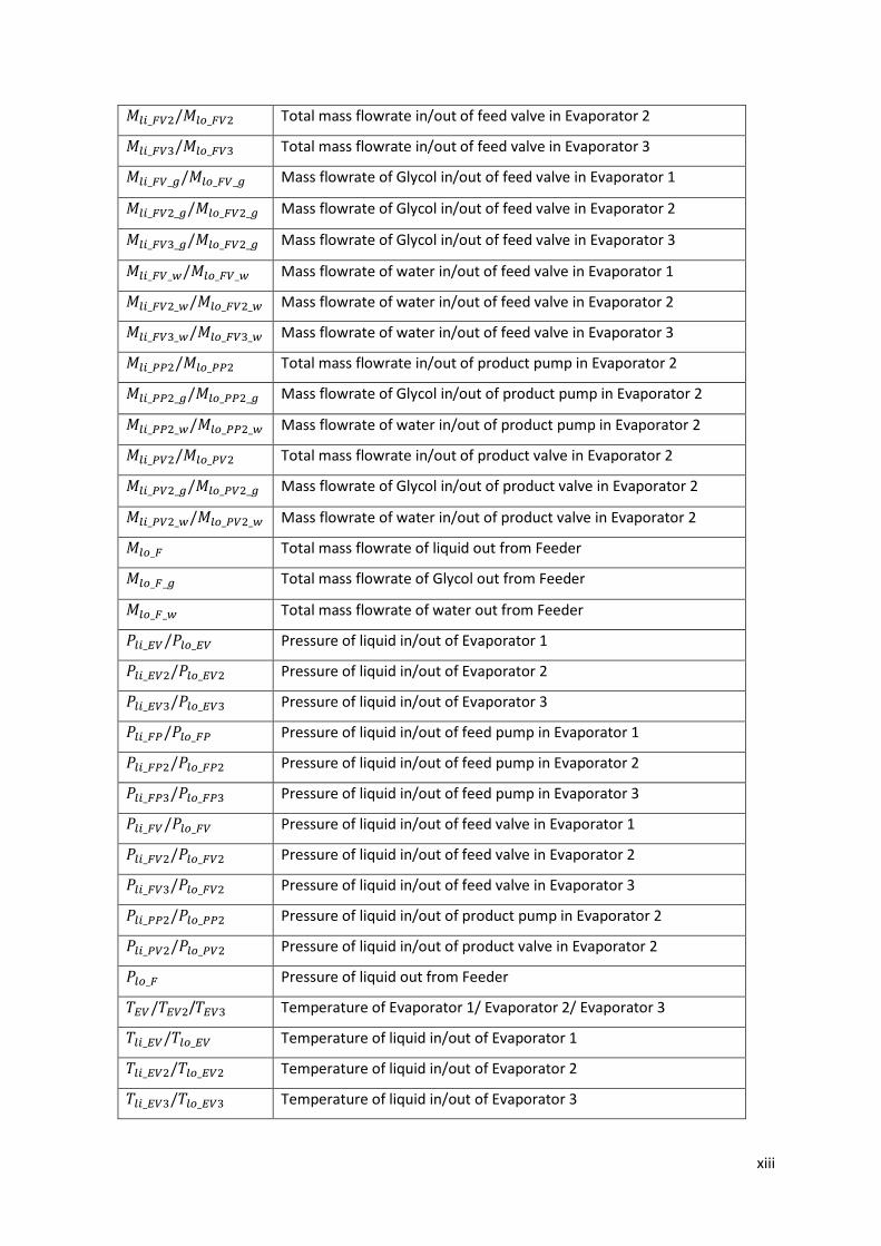
xiii
𝑀𝑀𝑙𝑙𝑠𝑠_𝐹𝐹𝐸𝐸2/𝑀𝑀𝑙𝑙𝑠𝑠_𝐹𝐹𝐸𝐸2 Total mass flowrate in/out of feed valve in Evaporator 2
𝑀𝑀𝑙𝑙𝑠𝑠_𝐹𝐹𝐸𝐸3/𝑀𝑀𝑙𝑙𝑠𝑠_𝐹𝐹𝐸𝐸3 Total mass flowrate in/out of feed valve in Evaporator 3
𝑀𝑀𝑙𝑙𝑠𝑠_𝐹𝐹𝐸𝐸_𝑔𝑔/𝑀𝑀𝑙𝑙𝑠𝑠_𝐹𝐹𝐸𝐸_𝑔𝑔 Mass flowrate of Glycol in/out of feed valve in Evaporator 1
𝑀𝑀𝑙𝑙𝑠𝑠_𝐹𝐹𝐸𝐸2_𝑔𝑔/𝑀𝑀𝑙𝑙𝑠𝑠_𝐹𝐹𝐸𝐸2_𝑔𝑔 Mass flowrate of Glycol in/out of feed valve in Evaporator 2
𝑀𝑀𝑙𝑙𝑠𝑠_𝐹𝐹𝐸𝐸3_𝑔𝑔/𝑀𝑀𝑙𝑙𝑠𝑠_𝐹𝐹𝐸𝐸2_𝑔𝑔 Mass flowrate of Glycol in/out of feed valve in Evaporator 3
𝑀𝑀𝑙𝑙𝑠𝑠_𝐹𝐹𝐸𝐸_𝑤𝑤/𝑀𝑀𝑙𝑙𝑠𝑠_𝐹𝐹𝐸𝐸_𝑤𝑤 Mass flowrate of water in/out of feed valve in Evaporator 1
𝑀𝑀𝑙𝑙𝑠𝑠_𝐹𝐹𝐸𝐸2_𝑤𝑤/𝑀𝑀𝑙𝑙𝑠𝑠_𝐹𝐹𝐸𝐸2_𝑤𝑤 Mass flowrate of water in/out of feed valve in Evaporator 2
𝑀𝑀𝑙𝑙𝑠𝑠_𝐹𝐹𝐸𝐸3_𝑤𝑤/𝑀𝑀𝑙𝑙𝑠𝑠_𝐹𝐹𝐸𝐸3_𝑤𝑤 Mass flowrate of water in/out of feed valve in Evaporator 3
𝑀𝑀𝑙𝑙𝑠𝑠_𝐹𝐹𝐹𝐹2/𝑀𝑀𝑙𝑙𝑠𝑠_𝐹𝐹𝐹𝐹2 Total mass flowrate in/out of product pump in Evaporator 2
𝑀𝑀𝑙𝑙𝑠𝑠_𝐹𝐹𝐹𝐹2_𝑔𝑔/𝑀𝑀𝑙𝑙𝑠𝑠_𝐹𝐹𝐹𝐹2_𝑔𝑔 Mass flowrate of Glycol in/out of product pump in Evaporator 2
𝑀𝑀𝑙𝑙𝑠𝑠_𝐹𝐹𝐹𝐹2_𝑤𝑤/𝑀𝑀𝑙𝑙𝑠𝑠_𝐹𝐹𝐹𝐹2_𝑤𝑤 Mass flowrate of water in/out of product pump in Evaporator 2
𝑀𝑀𝑙𝑙𝑠𝑠_𝐹𝐹𝐸𝐸2/𝑀𝑀𝑙𝑙𝑠𝑠_𝐹𝐹𝐸𝐸2 Total mass flowrate in/out of product valve in Evaporator 2
𝑀𝑀𝑙𝑙𝑠𝑠_𝐹𝐹𝐸𝐸2_𝑔𝑔/𝑀𝑀𝑙𝑙𝑠𝑠_𝐹𝐹𝐸𝐸2_𝑔𝑔 Mass flowrate of Glycol in/out of product valve in Evaporator 2
𝑀𝑀𝑙𝑙𝑠𝑠_𝐹𝐹𝐸𝐸2_𝑤𝑤/𝑀𝑀𝑙𝑙𝑠𝑠_𝐹𝐹𝐸𝐸2_𝑤𝑤 Mass flowrate of water in/out of product valve in Evaporator 2
𝑀𝑀𝑙𝑙𝑠𝑠_𝐹𝐹 Total mass flowrate of liquid out from Feeder
𝑀𝑀𝑙𝑙𝑠𝑠_𝐹𝐹_𝑔𝑔 Total mass flowrate of Glycol out from Feeder
𝑀𝑀𝑙𝑙𝑠𝑠_𝐹𝐹_𝑤𝑤 Total mass flowrate of water out from Feeder
𝑃𝑃𝑙𝑙𝑠𝑠_𝐸𝐸𝐸𝐸/𝑃𝑃𝑙𝑙𝑠𝑠_𝐸𝐸𝐸𝐸 Pressure of liquid in/out of Evaporator 1
𝑃𝑃𝑙𝑙𝑠𝑠_𝐸𝐸𝐸𝐸2/𝑃𝑃𝑙𝑙𝑠𝑠_𝐸𝐸𝐸𝐸2 Pressure of liquid in/out of Evaporator 2
𝑃𝑃𝑙𝑙𝑠𝑠_𝐸𝐸𝐸𝐸3/𝑃𝑃𝑙𝑙𝑠𝑠_𝐸𝐸𝐸𝐸3 Pressure of liquid in/out of Evaporator 3
𝑃𝑃𝑙𝑙𝑠𝑠_𝐹𝐹𝐹𝐹/𝑃𝑃𝑙𝑙𝑠𝑠_𝐹𝐹𝐹𝐹 Pressure of liquid in/out of feed pump in Evaporator 1
𝑃𝑃𝑙𝑙𝑠𝑠_𝐹𝐹𝐹𝐹2/𝑃𝑃𝑙𝑙𝑠𝑠_𝐹𝐹𝐹𝐹2 Pressure of liquid in/out of feed pump in Evaporator 2
𝑃𝑃𝑙𝑙𝑠𝑠_𝐹𝐹𝐹𝐹3/𝑃𝑃𝑙𝑙𝑠𝑠_𝐹𝐹𝐹𝐹3 Pressure of liquid in/out of feed pump in Evaporator 3
𝑃𝑃𝑙𝑙𝑠𝑠_𝐹𝐹𝐸𝐸/𝑃𝑃𝑙𝑙𝑠𝑠_𝐹𝐹𝐸𝐸 Pressure of liquid in/out of feed valve in Evaporator 1
𝑃𝑃𝑙𝑙𝑠𝑠_𝐹𝐹𝐸𝐸2/𝑃𝑃𝑙𝑙𝑠𝑠_𝐹𝐹𝐸𝐸2 Pressure of liquid in/out of feed valve in Evaporator 2
𝑃𝑃𝑙𝑙𝑠𝑠_𝐹𝐹𝐸𝐸3/𝑃𝑃𝑙𝑙𝑠𝑠_𝐹𝐹𝐸𝐸2 Pressure of liquid in/out of feed valve in Evaporator 3
𝑃𝑃𝑙𝑙𝑠𝑠_𝐹𝐹𝐹𝐹2/𝑃𝑃𝑙𝑙𝑠𝑠_𝐹𝐹𝐹𝐹2 Pressure of liquid in/out of product pump in Evaporator 2
𝑃𝑃𝑙𝑙𝑠𝑠_𝐹𝐹𝐸𝐸2/𝑃𝑃𝑙𝑙𝑠𝑠_𝐹𝐹𝐸𝐸2 Pressure of liquid in/out of product valve in Evaporator 2
𝑃𝑃𝑙𝑙𝑠𝑠_𝐹𝐹 Pressure of liquid out from Feeder
𝑇𝑇𝐸𝐸𝐸𝐸/𝑇𝑇𝐸𝐸𝐸𝐸2/𝑇𝑇𝐸𝐸𝐸𝐸3 Temperature of Evaporator 1/ Evaporator 2/ Evaporator 3
𝑇𝑇𝑙𝑙𝑠𝑠_𝐸𝐸𝐸𝐸/𝑇𝑇𝑙𝑙𝑠𝑠_𝐸𝐸𝐸𝐸 Temperature of liquid in/out of Evaporator 1
𝑇𝑇𝑙𝑙𝑠𝑠_𝐸𝐸𝐸𝐸2/𝑇𝑇𝑙𝑙𝑠𝑠_𝐸𝐸𝐸𝐸2 Temperature of liquid in/out of Evaporator 2
𝑇𝑇𝑙𝑙𝑠𝑠_𝐸𝐸𝐸𝐸3/𝑇𝑇𝑙𝑙𝑠𝑠_𝐸𝐸𝐸𝐸3 Temperature of liquid in/out of Evaporator 3

xiv
𝑇𝑇𝑙𝑙𝑠𝑠_𝐹𝐹𝐹𝐹/𝑇𝑇𝑙𝑙𝑠𝑠_𝐹𝐹𝐹𝐹 Temperature of liquid in/out of feed pump in Evaporator 1
𝑇𝑇𝑙𝑙𝑠𝑠_𝐹𝐹𝐹𝐹2/𝑇𝑇𝑙𝑙𝑠𝑠_𝐹𝐹𝐹𝐹2 Temperature of liquid in/out of feed pump in Evaporator 2
𝑇𝑇𝑙𝑙𝑠𝑠_𝐹𝐹𝐹𝐹3/𝑇𝑇𝑙𝑙𝑠𝑠_𝐹𝐹𝐹𝐹3 Temperature of liquid in/out of feed pump in Evaporator 3
𝑇𝑇𝑙𝑙𝑠𝑠_𝐹𝐹𝐸𝐸/𝑇𝑇𝑙𝑙𝑠𝑠_𝐹𝐹𝐸𝐸 Temperature of liquid in/out of feed valve in Evaporator 1
𝑇𝑇𝑙𝑙𝑠𝑠_𝐹𝐹𝐸𝐸2/𝑇𝑇𝑙𝑙𝑠𝑠_𝐹𝐹𝐸𝐸2 Temperature of liquid in/out of feed valve in Evaporator 2
𝑇𝑇𝑙𝑙𝑠𝑠_𝐹𝐹𝐸𝐸3/𝑇𝑇𝑙𝑙𝑠𝑠_𝐹𝐹𝐸𝐸3 Temperature of liquid in/out of feed valve in Evaporator 3
𝑇𝑇𝑙𝑙𝑠𝑠_𝐹𝐹𝐹𝐹2/𝑇𝑇𝑙𝑙𝑠𝑠_𝐹𝐹𝐹𝐹2 Temperature of liquid in/out of product pump in Evaporator 2
𝑇𝑇𝑙𝑙𝑠𝑠_𝐹𝐹𝐸𝐸2/𝑇𝑇𝑙𝑙𝑠𝑠_𝐹𝐹𝐸𝐸2 Temperature of liquid in/out of product valve in Evaporator 2
𝑇𝑇𝑙𝑙𝑠𝑠_𝐹𝐹 Temperature of liquid out from Feeder
𝑋𝑋𝑠𝑠_𝐸𝐸𝐸𝐸/𝑋𝑋𝑠𝑠_𝐸𝐸𝐸𝐸 Concentration of liquid in/out of Evaporator 1
𝑋𝑋𝑠𝑠_𝐸𝐸𝐸𝐸2/𝑋𝑋𝑠𝑠_𝐸𝐸𝐸𝐸2 Concentration of liquid in/out of Evaporator 2
𝑋𝑋𝑠𝑠_𝐸𝐸𝐸𝐸3/𝑋𝑋𝑠𝑠_𝐸𝐸𝐸𝐸3 Concentration of liquid in/out of Evaporator 3
𝑋𝑋𝑠𝑠_𝐹𝐹𝐹𝐹/𝑋𝑋𝑠𝑠_𝐹𝐹𝐹𝐹 Concentration of liquid in/out of feed pump in Evaporator 1
𝑋𝑋𝑠𝑠_𝐹𝐹𝐹𝐹2/𝑋𝑋𝑠𝑠_𝐹𝐹𝐹𝐹2 Concentration of liquid in/out of feed pump in Evaporator 2
𝑋𝑋𝑠𝑠_𝐹𝐹𝐹𝐹3/𝑋𝑋𝑠𝑠_𝐹𝐹𝐹𝐹3 Concentration of liquid in/out of feed pump in Evaporator 3
𝑋𝑋𝑠𝑠_𝐹𝐹𝐸𝐸/𝑋𝑋𝑠𝑠_𝐹𝐹𝐸𝐸 Concentration of liquid in/out of feed valve in Evaporator 1
𝑋𝑋𝑠𝑠_𝐹𝐹𝐸𝐸2/𝑋𝑋𝑠𝑠_𝐹𝐹𝐸𝐸2 Concentration of liquid in/out of feed valve in Evaporator 2
𝑋𝑋𝑠𝑠_𝐹𝐹𝐸𝐸2/𝑋𝑋𝑠𝑠_𝐹𝐹𝐸𝐸3 Concentration of liquid in/out of feed valve in Evaporator 3
𝑋𝑋𝑠𝑠_𝐹𝐹𝐹𝐹2/𝑋𝑋𝑠𝑠_𝐹𝐹𝐹𝐹2 Concentration of liquid in/out of product pump in Evaporator 2
𝑋𝑋𝑠𝑠_𝐹𝐹𝐸𝐸2/𝑋𝑋𝑠𝑠_𝐹𝐹𝐸𝐸2 Concentration of liquid in/out of product valve in Evaporator 2
𝑋𝑋𝑠𝑠_𝐹𝐹 Concentration of liquid out from Feeder
1
1.0 Introduction
This study case is choosing evaporation process as the focal point that will be investigated. Plus,
this project is carried out based on the case study examples that are provided by Aspen Custom
Modeler (ACM). The case study is about diluted glycol solution, which goes through a double
effect evaporation process to produce a more concentrated solution. Thorough study and
analysis are required to all models involved to rebuild those models in different software
packages. Upon completing the double evaporator effect in different software packages, a single
and triple effect model will be developed and tested. The needs of rebuilding the example in
different software packages come when in certain situations; ACM is too costly to be obtained.
The presence of these rebuild models could help to simulate an evaporator system with an easy
gain software such as Microsoft Excel.
A short introduction to the raw material chosen in the case study, glycol is one of the famous
products produced through evaporation process. The glycol production usually will start with
mixing the raw material of glycol with water. Next, the mixture will go through several stages of
the evaporation process. A number of evaporators used in the evaporation stage are specifically
designed to produce the desired concentration of glycol. The glycol product is widely used in the
automotive industry as a coolant solvent and essential element used in chemical industry.
Finally, the project report will cover:
Chapter 1: Introduction
This section will introduce the primary aim of the project and layout of the thesis
Chapter 2: Literature Review
In this chapter, all available types of the evaporators and manufacture processes of glycol in the
industry will be presented briefly as well as the software packages used together with the method
used in each software to develop the simulation.
Chapter 3: Project Objective and Scope
The scope and aim of the project are explicitly defined.

2
Chapter 4: Case Study Description and Model Development
This chapter will explain briefly about the case study and the model equations that are used in
the single and multiple effects of the evaporator, an imitator of the real industrial process used to
produce more concentrated glycol solution.
Chapter 5: Research Methodology
Here, the method of applying, testing and evaluating the model for single and multiple effect
evaporators will be explained.
Chapter 6: Results
The results of steady-state simulation and optimisation are presented, compared and discussed in
this chapter.
Chapter 7: Conclusion and Future Work
The summarisation of the project is explained in this chapter as well as future work
recommended for future students.

3
2.0 Literature Review
A literature review is carried out to give a better overview of the research and a deeper
explanation of the overall system implemented in the case study. As far as the research
continues, the thesis is done based on the example in Aspen Custom Modeler (ACM). Again, the
example is a double evaporator system for a dilute glycol solution, which is to produce more
concentrated glycol solution.
Any organic compound that belongs to the alcohol family, which has two hydroxyls (-OH) group
attached to different carbon atoms will be called as glycol (Britannica 2015). Generally, the term
is applied to the simplest member of the class that is ethylene glycol. Another famous member of
the glycol family that is widely produced in the industry is propylene glycol (Britannica 2015).
Both compounds play different function in different industry. Ethylene, a mildly toxic component,
is a well-known component in the automobile industry that usually acts as an antifreeze in an
automobile cooling system or as brake fluid, whereas propylene glycol is a non-toxic component
and an excellent solvent that is used extensively in foods, cosmetics, and oral hygiene products.
The evaporation process is involved in manufacturing both components. Most of the
manufacturers of this component will use a multi-effect evaporator system to produce the
suitable concentration that is demanded by the market. Evaporation is a process by which a
substance in the liquid tends to convert into the gaseous phase without reaching its boiling point
(Pabasara 2017). The evaporated solvent, which will be eliminated from the liquid, mostly water,
will then produce to a more concentrated product. The process happens when the intermolecular
bonds in the liquid absorb enough heat to dissociate and release the molecules into the gaseous
phase (Pabasara 2017). Evaporation process only occurs below the boiling point and on the
surface of the liquid. Molecules on the surface of the liquid will absorb heat from the atmosphere
and break the intermolecular bond and change its phase to gas (Pabasara 2017). The fact that
evaporation process also undergoes a vaporized process makes most of the people assume that
evaporation and distillation is a similar process. By contrast, distillation is a modern separation
technique and the separation happened at the specific boiling point of liquids. However, not in
evaporation process where it could start although the liquid is not reaching the boiling point.
Table 1 shows the difference between an evaporation process and distillation process.
4
Table 1 Evaporation versus Distillation Process(Pabasara 2017)
Evaporation Distillation
Evaporation is the process of transforming
liquid into gas, under the influence of heat
Distillation involves obtaining gas or vapour
from liquids by heating and condensing to
liquid
Only occurs on the surface Does not occur only on the surface
Liquid vaporizes below boiling point Liquid vaporizes at boiling point
A slow process Rapid process
Not a separation technique A separation technique
The evaporator is a tool used to make the evaporation process in the industry and is used in a
wide range of industries, such as pharmaceuticals, food, and beverages, chemicals, and more. The
principle utilised in the evaporator is high pressure and temperature of steam, which acts as the
heat supplier that is fed into the evaporator. Heat from the steam will increase the temperature
of the evaporator, and at specific high temperature, water in the liquid will start to vaporize, and
a more concentrated product will be produced from the evaporator. Besides the concentrated
solution, evaporated steam is also considered as a product of the evaporator. In a multi-effect
evaporator system, the vaporized steam will then be recycled and used for the next evaporator.
There are various types of evaporators in which each has their own processing technique in the
industry. Sub-chapters below give details regarding the types of evaporators that are available in
the industry.
2.1 Types of Evaporators
a) Batch pan
One of the oldest methods to concentrate a liquid is by using an evaporator. Although the
batch pan method is outdated compared to current technology, the batch pan is still used
in a few limited applications such as concentrating jams and jellies (APV 2008). Due to its
vessel shapes, as shown in Figure 1, the batch pan has a small heat transfer area and heat

5
transfer coefficient. Hence, the batch pan evaporator has a small and limited capacity of
evaporating a product.
Figure 1 Batch Pan Evaporator (APV 2008)
b) Tubular Evaporator
i. Natural Circulation
The use of a short tube bundle within the batch pan or an external shell and tube heater
outside of the main vessel will allow the natural circulation evaporator to be successfully
operated. The advantage of having external heater is the size of the heater does not
depend on the size or shape of the vessel (APV 2008). Usually, this type of evaporator is
used as a base of the distillation column.
Figure 2 Natural Circulation Evaporator (APV 2008)
6
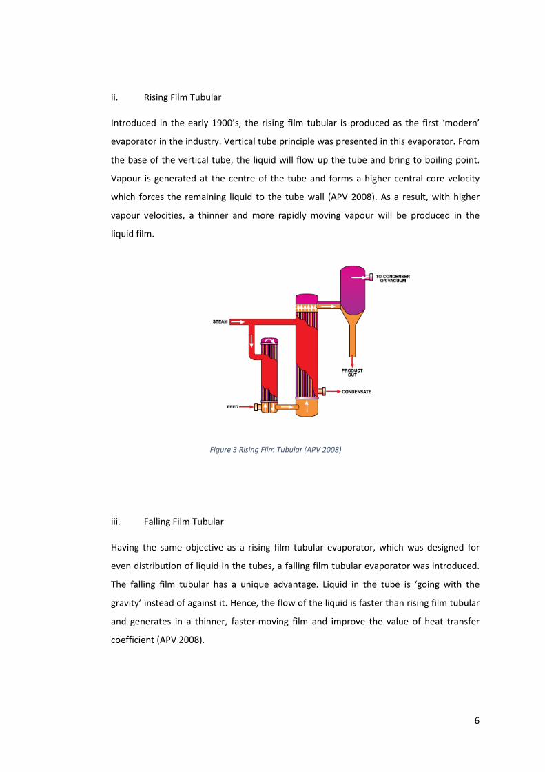
ii. Rising Film Tubular
Introduced in the early 1900’s, the rising film tubular is produced as the first ‘modern’
evaporator in the industry. Vertical tube principle was presented in this evaporator. From
the base of the vertical tube, the liquid will flow up the tube and bring to boiling point.
Vapour is generated at the centre of the tube and forms a higher central core velocity
which forces the remaining liquid to the tube wall (APV 2008). As a result, with higher
vapour velocities, a thinner and more rapidly moving vapour will be produced in the
liquid film.
Figure 3 Rising Film Tubular (APV 2008)
iii. Falling Film Tubular
Having the same objective as a rising film tubular evaporator, which was designed for
even distribution of liquid in the tubes, a falling film tubular evaporator was introduced.
The falling film tubular has a unique advantage. Liquid in the tube is ‘going with the
gravity’ instead of against it. Hence, the flow of the liquid is faster than rising film tubular
and generates in a thinner, faster-moving film and improve the value of heat transfer
coefficient (APV 2008).

7
Figure 4 Falling film tubular (APV 2008)
iv. Forced Circulation
This design was established for processing liquors, which are susceptible to scaling or
crystallizing. The liquid is circulated at a high rate through all components in the system
and prevented from reaching the boiling point (APV 2008). Once the liquid enters the
separator, the liquid flashes and vapour are produced due to the absolute pressure is
slightly less than in the tube bundles. High recirculation rates minimize the deposition of
crystal along the heating surface.
Figure 5 Force Circulation Evaporator (APV 2008)

8
c) Plate Type Evaporator
i. Rising/Falling Film Plate
Working principle of the rising/falling film plate evaporator (RFFPE) involved the use of a
number of plate packs or units (APV 2008). Each plate or unit will consist two steam
plates and two product plates in Figure 6 below.
Figure 6 Rising/falling Film Plate evaporator design (APV 2008)
The product is fed through parallel feed ports and distributed equally to each of rising
film annuli. Heat is transferred from the adjacent steam path with the vapours. During
the operation, partially concentrated liquid mixture transfers to a ‘slot’ above one of the
adjacent steam. Next, the mixture enters the falling film with the assistance of gravity and
completes the evaporation process (APV 2008). Moreover, the rising/falling film can be
adapted as multi-effect evaporators.
ii. Falling Film Plate
Adapting the same principle as the rising/falling film plate, however, the falling film plate
has a significant innovation. A patented feed distribution is shown in Figure 7.

9
Figure 7 Patented feed distribution system (APV 2008)
The advantage of this new feature is the flow of liquid during the evaporation is more
even and stable (APV 2008). Furthermore, the unique feature of this evaporator is the
capability to operate the system in series or parallel.
Next sections will explain further about the manufacturing process of ethylene glycol and
propylene glycol where the principle of producing this product is applied in the research as well
as the software used during the research.
2.2 Ethylene Glycol Manufacturing Process
There are two processes of manufacturing ethylene that has been introduced in the industry. The
first process is based on the reaction of formaldehyde with carbon monoxide (Jr 1984). This
practice has been discontinued from 1968 and replaced by the second method that is the
hydration of ethylene oxide. The second method by far has become the basis for producing
ethylene glycol from 1968 until today. In 1979, 800 million lb/year of ethylene had been produced
in the United States using the hydration method (Jr 1984). Figure 8 shows the schematic flow
diagram of the ethylene oxide hydration plant and the plant was designed to maximise the
production of monoethylene glycol.

10
Figure 8 Commercial ethylene oxide hydration plant (Jr 1984)
The plant starts with refining both ethylene oxide and pure water as raw material. Pure water is
coming from the mix of makeup water and recycled water. A mixture of purified water and
ethylene oxide is then pumped to the reactor after being preheated by the recycled hot water
and steam. In the reactor, the operating pressure and temperature are controlled at 14-22 atm
and 190-200℃. The reason for controlling the pressure and temperature of the reactor is to avoid
vaporization of ethylene oxide from the aqueous solution. However, both temperature and
pressure depend on the initial concentration of the oxide.
The water-glycol solution is fed into the first stage of multiple stages of evaporator where those
evaporators will recycle the high-pressure steam back into the system. Typically, the last
remaining stages of the evaporator will operate at a lower pressure and at vacuum state in the
final stage. The evaporated water is recovered as the condensate and recycled back to the mixing
tank (J. McKetta Jr, 1984). Finally, the concentrated crude glycol will then fraction in a series of
vacuum distillation towers to produce purified mono-ethylene glycol, and it’s a by-product.

11
2.3 Propylene Glycol Manufacturing Process
Propylene glycol, C3H8O2, also known as propane-1,2-diol, is colourless and odourless organic
compound (Patel 2009). The same method as the ethylene glycol is used to produce propylene
glycol. Generally, the design of the plant that produces the propylene glycol is identical to the
ethylene glycol plant. Figure 9 shows the design plant for producing propylene glycol.
Figure 9 Propylene Glycol Process Plant (Patel 2009)
The only difference between the ethylene glycol and propylene glycol is the raw material used to
produce both compounds. The raw material used for producing propylene glycol is propylene
oxide. Again, this compound will be mixed in the reactor. The reaction of the mixture will take
place at 120-190℃, and the pressure has to be maintained at 2170 kPa (Patel 2009). This mixture
will go through multiple stages of the evaporator, which are supplied with high-pressure steam.
The evaporators will dehydrate the water in the mixture, and the mixture will then flow to drying
tower to eliminate the excessive water. In the last stage of this process, the mixture will go
through a distillation column for separation and purification of the glycol (Patel 2009).
The primary purpose of explaining both processes is to show that the example given from the
ACM is a real process that takes place in the industry. Understanding the principles used in the
case study from ACM will help to understand the principle used of the evaporator in the industry.
With the knowledge gained from the ACM’s example, a model can be constructed in Matlab and
Microsoft Excel. Sequential modular operation, a different method of solving the equation is the
reason a model of double effect evaporator has to be built in both software. In an evaporation
system, many equations are involved such as energy balance equations, mass balance equations,
pressure, temperature, etc. The ACM can solve these equations simultaneously with the

12
condition that the degree of freedom (DOF) in the evaporator is equal to zero. On the contrary,
Microsoft Excel will solve the equations that are involved in evaporation process sequentially. In
Matlab however, both methods can be used. Similarly, for the sequential method, Matlab is using
the same technique as in Microsoft Excel, but for the simultaneous method, an ‘FSolve’ function
is used. Though the ‘FSolve’ can solve the equations simultaneously, some constraints cannot be
applied as in the ACM because ‘FSolve’ function does not provide any constraint parameters.
Chapter 2.4, 2.5 & 2.6 will elaborate on the software used in the research, namely Aspen Custom
Modeler (ACM), Matlab and Microsoft Excel while chapter 2.7 will explain on the sequential and
simultaneous principle.
2.4 Aspen Custom Modeler (ACM)
ACM is easy-to-use software that enables the user to create, edit and re-use models of the
processing unit. The software operates by building a simulation application that combines all the
models on a graphical flowsheet. The models can be used from the software library or created
and then be stored in the software library for distribution and use. The interesting part of this
software is the model that has been built can run in either dynamic, steady-state, parameter
estimation or optimisation simulation which provides flexibility and power. There are only a few
software that could perform these features, and that is one of the reasons ACM is so prevalent in
the process industry. Also, ACM can be customised and has extensive automation features, which
make it easy to combine with other products such as Microsoft Excel and Visual Basic.
2.5 Matlab (Matrix Laboratory)
Matlab is an interactive software that is widely used in science and engineering field for
numerical computation and data visualization. Matlab combines mathematical computing,
visualization and a powerful language that provides a flexible platform for technical computing
(Dukkipati 2009). Known for friendly user interphase and highly optimised matrix and vector
calculation, Matlab becomes one of the preferable software in doing modelling and simulation.
That is also the reason why Matlab is chosen to be one of the software in doing this research.
Matlab can perform both simultaneous and sequential solving method. Nevertheless, in solving
13
simultaneously, no constraint could be applied, and this makes the result in Matlab less accurate
compared to ACM.
2.6 Microsoft Excel
Microsoft Excel, one of the well-known product of Microsoft, is an electronic spreadsheet
program that is usually used for storing, organizing and manipulating data (French 2016). Initially,
Microsoft Excel was created for accounting purposes, but with updates and modifications,
Microsoft Excel became a new platform for solving mathematical modelling. Mathematical
modelling can be addressed by using the built-in solver, which is designed to carry out a broad
range calculation. However, there is a limitation in using the Microsoft Excel whereby it cannot
perform a simultaneous solving method as mentioned before. Thus, to perform the model,
proper and systemic equations are needed, and the results then can be compared with other
software.
Once all models in the three software are completed, the result of the test in each software will
be compared. The test will include a test in steady-state, dynamic, and optimisation mode. The
performance of each software will be studied and investigated.
2.7 Sequential Modular Operation
This method is used to solve multiple equations that are related to each other a step by step. To
perform a steady-state simulation, many model equations are involved, and some of the
equations are related to each other. A steady-state simulation by sequential modular operation
means that any essential equations have to be solved first, and if fail to do so, the other
equations cannot be resolved. Hence, the steady-state simulation cannot be performed. This
principle is used in Microsoft Excel and Matlab normal calculation operation.

14
On the contrary, simultaneous modular operation is when the solver can solve two or three
equations at the same time, even though the equations are related. This principle is used in
running simulation in ACM and ‘FSolve’ tool.
3.0 Project Objective and Scope
The project is based on the case study in the examples provided by Aspen Custom Modeller
(ACM), in which a glycol solution is fed through a double effect evaporator to become a more
concentrated and valuable glycol solution. The case study uses a similar method that has been
utilised in the industry to recover glycol. With this approach, the extra cost of purchasing the
additional glycol could be prevented. Thus, the primary aim of this project is to optimise the
process by comparing the performances of single, double, and triple effect evaporators and to do
so, the model equations written for double effect evaporators in ACM should be thoroughly
studied to gain a deep understanding of the process. From this knowledge, similar programs will
be developed and applied to single and triple effect evaporators.
A steady-state model will be built in Matlab and Microsoft Excel first to test the performances of
the solver of each software packages. Steady-state simulation can be done in all three packages
but will only report in details using the software, having a more efficient solver, which can
produce trustworthy results. Once satisfied with the performance of the steady-state simulation,
the case study continues with developing the optimisation in all three packages.
Some main outcomes of the project are:
1. Be able to apply all engineering knowledge and skills gained in the past year of learning at
Murdoch University in designing an industry-like process.
2. Be able to improve skill using different software packages and technical report writing
skills.

15
4.0 Case Study Description and Model Development
The given project is based on a case study taken from ACM. Initially the model was developed for
the double effect evaporators. From the ACM code, mathematical equations used in the model
were written for a single effect then modified for a multiple effect as shown in the following
sections. Next, the development of a single effect evaporator will be presented and then followed
by an adaptation of the single effect evaporator to multiple effect evaporators’ model.
4.1 Single Effect Evaporator
Figure 10 Flow diagram of single effect evaporator
The flow diagram of a single evaporator is shown in Figure 10. The steam supply is available to
provide saturated steam at 105ᵒC. The pressure of the saturated steam can be obtained by using
Eq. (1), which gives the same result as in any saturated steam table.
𝑃𝑃𝑠𝑠𝑠𝑠 = 0.1333 × 10�7.96681− 166821𝑇𝑇𝑠𝑠𝑠𝑠+228
� (1)
𝑃𝑃𝑠𝑠𝑠𝑠 is obtained respectively in Eq. (1) when 𝑇𝑇𝑠𝑠𝑠𝑠 = 105ᵒC. From the steam supply, the saturated
steam flows through a steam valve and defined by Eq. (2), where the steam mass flow rate, 𝑚𝑚𝑠𝑠𝑠𝑠,
of the saturated steam can be calculated and the valve coefficient, 𝐾𝐾𝑠𝑠𝑙𝑙, is initially fixed at
46.361𝑚𝑚3
ℎ.
𝑚𝑚𝑠𝑠𝑠𝑠𝑖𝑖 = 𝑚𝑚𝑠𝑠𝑠𝑠𝑜𝑜 = �𝐾𝐾𝑠𝑠𝑙𝑙 × �𝑃𝑃𝑠𝑠𝑠𝑠𝑖𝑖 − 𝑃𝑃𝑠𝑠𝑠𝑠𝑜𝑜� (2)
The liquor in Figure 10 is shown as the liquid feeder to the evaporator. An aqueous solution of
3.5w% glycol is pumped to the liquid valve. The solution is sub-cooled to 88ᵒC and maintained at
100kPa. Both pressure, 𝑃𝑃𝑙𝑙𝑖𝑖 and temperature, 𝑇𝑇𝑙𝑙𝑖𝑖 of the glycol solution are expressed in a

16
correlation presented in Eq. (3). The mathematical model for the liquid pump and liquid valve are
shown in Eq. (4) and (5). In Eq. (3), X represents glycol mass fraction while MW represents glycol
molar mass.
𝑃𝑃𝑙𝑙𝑖𝑖 = 0.1333 × ��1−𝑋𝑋𝑖𝑖�𝑀𝑀𝑀𝑀𝑤𝑤
�1−𝑋𝑋𝑖𝑖�𝑀𝑀𝑀𝑀𝑤𝑤
+ 𝑋𝑋𝑖𝑖𝑀𝑀𝑀𝑀𝑔𝑔
�10�7.96681− 166821
𝑇𝑇𝑙𝑙𝑖𝑖+228� (3)
∆𝑃𝑃 = 𝑃𝑃𝑙𝑙𝑜𝑜 − 𝑃𝑃𝑙𝑙𝑖𝑖 (4)
𝑚𝑚𝑙𝑙𝑖𝑖 = 𝑚𝑚𝑙𝑙𝑜𝑜 = �𝐾𝐾𝑙𝑙𝑙𝑙 × �𝑃𝑃𝑙𝑙𝑖𝑖 − 𝑃𝑃𝑙𝑙𝑜𝑜� (5)
Molar masses of glycol and water are 62 and 18.02 respectively use in this case study, and the
liquid valve coefficient is set at 185𝑚𝑚3
ℎ. Around the evaporator, the total mass and glycol balances
are given in Eq. (6) and (7); while the energy balances are shown in Eq. (8) and (9).
𝑚𝑚𝑙𝑙𝑖𝑖 = 𝑚𝑚𝑙𝑙𝑜𝑜 + 𝑚𝑚𝑙𝑙𝑣𝑣𝑜𝑜 (6)
𝑋𝑋𝑠𝑠𝑚𝑚𝑙𝑙𝑖𝑖 = 𝑋𝑋𝑠𝑠𝑚𝑚𝑙𝑙𝑜𝑜 (7)
𝑚𝑚𝑙𝑙𝑖𝑖�𝐻𝐻�𝑙𝑙𝑖𝑖 − 𝐻𝐻�𝑙𝑙𝑜𝑜� = 𝑚𝑚𝑙𝑙𝑣𝑣𝑜𝑜�𝐻𝐻�𝑙𝑙𝑣𝑣𝑜𝑜 − 𝐻𝐻�𝑙𝑙𝑜𝑜� + 𝑚𝑚𝑠𝑠𝑠𝑠𝜆𝜆 (8)
𝑚𝑚𝑠𝑠𝑠𝑠𝜆𝜆 = 𝐻𝐻𝑠𝑠𝑡𝑡 × 𝐴𝐴𝑠𝑠𝑡𝑡 × ∆𝑇𝑇 (9)
λ : Heat condensation of steam 𝐴𝐴𝑠𝑠𝑡𝑡 : Heat transfer area 𝐻𝐻𝑠𝑠𝑡𝑡 : Heat transfer coefficient
In the above equations, λ is fixed at 2080.8kJ/kg. The 𝐴𝐴𝑠𝑠𝑡𝑡 and 𝐻𝐻𝑠𝑠𝑡𝑡 are respectively given as
145𝑚𝑚2 and 80kJ/ℎ.𝑚𝑚2.℃. The temperature difference between the heating medium and the
operating temperature in the evaporator is shown as ∆𝑇𝑇 (Linh T. T. Vu 2016).
To get the value of specific enthalpy of the liquid glycol solution and water vapor, equations in Eq.
(10) and (11) are used, where the reference temperature, 𝑇𝑇𝑟𝑟𝑟𝑟𝑡𝑡 is assumed to be 60℃, the heat
capacities of glycol and water are 2.4 and 4.183 kJ/kgᵒC respectively (Linh T. T. Vu 2016).
𝐻𝐻�𝑙𝑙𝑜𝑜 = 𝐻𝐻�𝑠𝑠𝑓𝑓𝑙𝑙 = �𝑇𝑇𝑠𝑠𝑓𝑓𝑙𝑙 − 𝑇𝑇𝑟𝑟𝑟𝑟𝑡𝑡� × ��1 − 𝑋𝑋𝑡𝑡𝑜𝑜�𝐶𝐶𝑣𝑣𝑤𝑤 + 𝑋𝑋𝑡𝑡𝑜𝑜𝐶𝐶𝑣𝑣𝑔𝑔� (10)
𝐻𝐻�𝑠𝑠𝑉𝑉𝑠𝑠𝑠𝑠 = �𝑇𝑇𝑠𝑠𝑉𝑉𝑠𝑠𝑠𝑠 − 𝑇𝑇𝑟𝑟𝑟𝑟𝑡𝑡�𝐶𝐶𝑣𝑣𝑤𝑤 + 𝜆𝜆 (11)
17
After leaving, the vapour flows through the vapour valve. The valve coefficient is set at 521.33 𝑚𝑚3
ℎ
at the beginning. The model of this valve is shown in Eq. (12). It is noted that the difference in
pressure is between the inlet liquid and the outlet vapour (Linh T. T. Vu 2016). The vapour that
leaves the first effect will be used in the double effect evaporator as to heat the second effect.
𝑚𝑚𝑙𝑙𝑣𝑣𝑜𝑜 = �𝐾𝐾𝐸𝐸𝑣𝑣𝑠𝑠 × �𝑃𝑃𝑙𝑙𝑖𝑖 − 𝑃𝑃𝑙𝑙𝑣𝑣𝑜𝑜� (12)
The product of this single effect is the concentrated glycol liquid. However, more concentrated
glycol liquid will be produced as the first effect concentrated glycol liquid is introduced to the
double effect evaporator for further water evaporation (Linh T. T. Vu 2016).
4.2 Multi Effect Evaporator
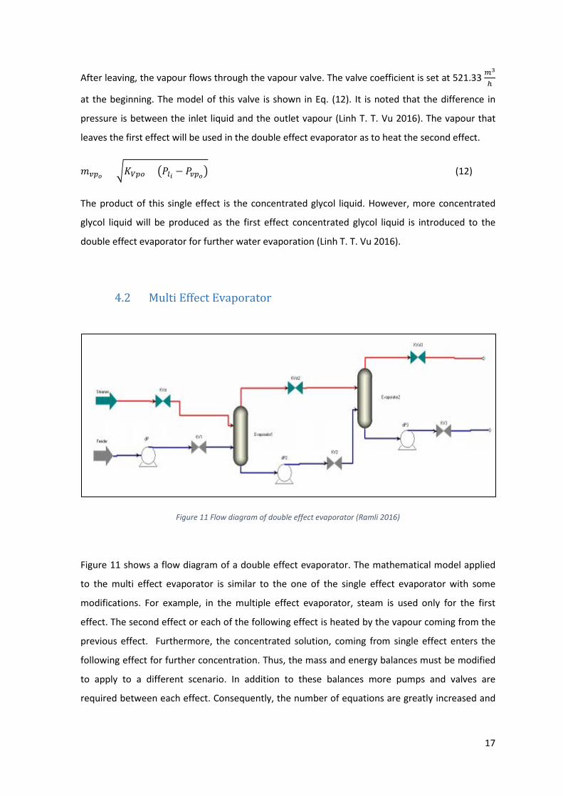
Figure 11 Flow diagram of double effect evaporator (Ramli 2016)
Figure 11 shows a flow diagram of a double effect evaporator. The mathematical model applied
to the multi effect evaporator is similar to the one of the single effect evaporator with some
modifications. For example, in the multiple effect evaporator, steam is used only for the first
effect. The second effect or each of the following effect is heated by the vapour coming from the
previous effect. Furthermore, the concentrated solution, coming from single effect enters the
following effect for further concentration. Thus, the mass and energy balances must be modified
to apply to a different scenario. In addition to these balances more pumps and valves are
required between each effect. Consequently, the number of equations are greatly increased and
18
solving these equations either simultaneously or sequentially still requires a reliable software
package with an efficient solver.
4.3 Optimisation
In ACM, optimisation for the evaporator example is done by minimising the objective function.
The objective function is summation of several costing equation which has been provided in the
ACM example. The costing equations are as below
𝐶𝐶𝐶𝐶𝐶𝐶𝐶𝐶1 = −(𝑋𝑋𝑠𝑠_𝐹𝐹2 ∗ 𝑀𝑀𝑙𝑙𝑠𝑠_𝐹𝐹 ∗ 700 ) (13)
𝐶𝐶𝐶𝐶𝐶𝐶𝐶𝐶2 = −(80 ∗ 𝑚𝑚𝑠𝑠𝑠𝑠) − (10 ∗ �101.3 − 𝑃𝑃𝑙𝑙𝑣𝑣𝐸𝐸𝑉𝑉2� ∗ 𝑚𝑚𝑙𝑙𝑣𝑣2) (14)
𝐶𝐶𝐶𝐶𝐶𝐶𝐶𝐶3 = −�95 ∗ 𝑀𝑀𝑙𝑙𝑠𝑠_𝐸𝐸𝐸𝐸2� + (𝑋𝑋𝑠𝑠_𝐸𝐸𝐸𝐸20.2 ∗ 𝑀𝑀𝑙𝑙𝑠𝑠_𝐸𝐸𝐸𝐸2 ∗ 700) (15)
𝐶𝐶𝐶𝐶𝐶𝐶𝐶𝐶4 = 𝑚𝑚𝑠𝑠𝑠𝑠 ∗ (𝑇𝑇𝑐𝑐ℎ𝑟𝑟𝑠𝑠𝑠𝑠 − 50) ∗ 0.7 (16)
𝐶𝐶𝐶𝐶𝐶𝐶𝐶𝐶5 = 𝑚𝑚𝑠𝑠𝑠𝑠2 ∗ (𝑇𝑇𝑐𝑐ℎ𝑟𝑟𝑠𝑠𝑠𝑠2 − 50) ∗ 0.7 (17)
𝑂𝑂𝑂𝑂𝑂𝑂𝑂𝑂𝑂𝑂𝐶𝐶𝑂𝑂𝑂𝑂𝑂𝑂𝑂𝑂𝑂𝑂𝑂𝑂𝑂𝑂𝐶𝐶𝑂𝑂𝐶𝐶𝑂𝑂 = 𝐶𝐶𝐶𝐶𝐶𝐶𝐶𝐶1 + 𝐶𝐶𝐶𝐶𝐶𝐶𝐶𝐶2 + 𝐶𝐶𝐶𝐶𝐶𝐶𝐶𝐶3 + 𝐶𝐶𝐶𝐶𝐶𝐶𝐶𝐶4 + 𝐶𝐶𝐶𝐶𝐶𝐶𝐶𝐶5 (18)
In order to calculate the equations calculation above where optimisation will be performed,
several variables will be selected. The chosen variables will affect the value of the variables used
in the costing equations. Further explanation of this step is elaborated in chapter 5.1.5.
5.0 Research Methodology
This section will explain thoroughly the step of applying, testing and evaluating of the model for
single and multiple effect evaporators by using different software packages. The flowchart in
Figure 12 shows the overall methodology used and step in building the model in the case study.
19
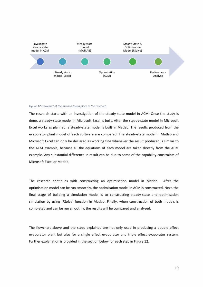
Figure 12 Flowchart of the method taken place in the research
The research starts with an investigation of the steady-state model in ACM. Once the study is
done, a steady-state model in Microsoft Excel is built. After the steady-state model in Microsoft
Excel works as planned, a steady-state model is built in Matlab. The results produced from the
evaporator plant model of each software are compared. The steady-state model in Matlab and
Microsoft Excel can only be declared as working fine whenever the result produced is similar to
the ACM example, because all the equations of each model are taken directly from the ACM
example. Any substantial difference in result can be due to some of the capability constraints of
Microsoft Excel or Matlab.
The research continues with constructing an optimisation model in Matlab. After the
optimisation model can be run smoothly, the optimisation model in ACM is constructed. Next, the
final stage of building a simulation model is to constructing steady-state and optimisation
simulation by using ‘FSolve’ function in Matlab. Finally, when construction of both models is
completed and can be run smoothly, the results will be compared and analysed.
The flowchart above and the steps explained are not only used in producing a double effect
evaporator plant but also for a single effect evaporator and triple effect evaporator system.
Further explanation is provided in the section below for each step in Figure 12.
Investigate steady state
model in ACM
Steady state model (Excel)
Steady state model
(MATLAB)
Optimisation (ACM)
Steady State & Optimisation
Model (FSolve)
Performance Analysis

20
5.1 Development and Testing the Model Equations
As mentioned earlier, the case study is based on the example in ACM and uses a simultaneous
modular operation to run the steady-state simulation. However, this method cannot be
implemented in Matlab and Microsoft Excel due to their modular operation constraint. In basic
Matlab operation and Microsoft Excel, the steady-state simulation only can be achieved by using
the sequential modular operation. A correct and proper arrangement of mathematical equations
is needed. Thus, a few investigations have to be done before constructing the steady-state
simulation model in Matlab and Microsoft Excel.
5.1.1 Collecting and Interpreting Data
All data that are obtained from the steady-state simulation example in ACM is recorded in a
Microsoft Excel spreadsheet. The purpose of collecting these data is to ensure the process of
analysing data from all models is more accessible and organized. Besides, the spreadsheet will
reduce the effort of tracing data by which the data is a fixed or calculated value.
Figure 13 Collection of data from double effect of evaporator in ACM
Figure 13 is one of the examples of data collected from ACM. Details of the data are attached in
Appendix A. In Figure 13, highlighted cells indicate a fixed value while the non-highlighted cells
are values obtained from the steady-state simulation. At the same time, the arrangement of each
data component in Excel is following the exact component arrangement in the ACM model.

21
Together with the arrow in the spreadsheet, this feature can help the user to understand the
process flow of the simulation without opening the simulation in ACM.
Table 2 below are all the fixed values used in the case study.
Table 2 Fixed process value from the example in ACM
Liquid Properties
Properties Specific Heat Capacity (Cp), 𝒌𝒌𝒌𝒌𝒌𝒌𝒌𝒌℃
Molar Mass, 𝒌𝒌𝒎𝒎𝒎𝒎𝒎𝒎
Glycol 2.4 18.02
Water 4.18 62.00
Physical Properties
First Effect of Evaporator Second Effect of Evaporator
Heat Transfer Area (Atf, Atf2),
𝑚𝑚2
168 145
Heat Transfer Coefficient (Htf,
Htf2), 𝑘𝑘𝑘𝑘ℎ.𝐾𝐾
150 80
Latent Heat of Water at 160ᵒC
(λ), 𝑘𝑘𝑘𝑘𝑘𝑘𝑔𝑔
2080.8 2080.8
Liquid Hold-Up
(Mhold,Mhold2), kg
3300 2500
Valve Properties
First Effect of Evaporator Second Effect of Evaporator
Steam Valve Coefficient (Ksv),
𝑚𝑚3
ℎ
46.361 -
Steam Valve Coefficient in the
Evaporator (Kvvp, Kvvp2), 𝑚𝑚3
ℎ
521.33 703.35
Liquid Valve Coefficient (Klv,
Klv2), 𝑚𝑚3
ℎ
185 -
Pump Properties
Pressure Differences Across the Pump (dP,dP2),

22
kPa
First Effect Evaporator Pump (In) 44.27
First Effect Evaporator (Out)/ Second Effect
Evaporator (In)
10.00
Second Effect Evaporator (out) 90.30
Here are some of the fixed process variable values used in the example model:
Mass fraction of Glycol out of feeder (𝑀𝑀𝑙𝑙𝑠𝑠_𝐹𝐹_𝑔𝑔) = 0.035 kgkg
Temperature of the steam out from steamer (𝑇𝑇𝑠𝑠𝑠𝑠_𝑆𝑆𝑆𝑆) = 105ºC
Temperature of the liquid out from Feeder (𝑇𝑇𝑙𝑙𝑠𝑠_𝐹𝐹) = 88ºC
Pressure liquid out from Feeder (𝑃𝑃𝑙𝑙𝑠𝑠_𝐹𝐹) = 100 kPa
Pressure liquid out from liquid valve in second effect evaporator (𝑃𝑃𝑙𝑙𝑠𝑠_𝐹𝐹𝐸𝐸2) = 120 kPa
Pressure steam out from second effect evaporator (𝑃𝑃𝑙𝑙𝑣𝑣_𝐸𝐸𝐸𝐸2) = 45 kPa
Based on the collected data in the early stage of simulation, three variables are detected that will
give a significant influence towards the simulation calculation. The variables identified are as
follow:
i. Mass flowrate of steam that feeds to the Evaporator, 𝑚𝑚𝑠𝑠𝑠𝑠
ii. Concentration of product in first effect evaporator, 𝑋𝑋𝑠𝑠_𝐸𝐸𝐸𝐸
iii. Concentration of product in second effect evaporator, 𝑋𝑋𝑠𝑠_𝐸𝐸𝐸𝐸2
On how these three variables can influence the overall simulation in ACM are elaborated further
in the investigation in Microsoft Excel section.
5.1.2 Investigation of Double Effect Evaporator Example in Aspen Custom Modeler
(ACM)
The modeling example in the case study is a mathematical description of the real industrial
processes by using a set of equations. Understanding and rebuilding the existing model in ACM is
the primary objective to achieve by constructing a new simulation in different software packages.
The best part of the ACM’s example program is the program simulates a real industry plant. All

23
the data and values produced from the example can be assumed as reasonable in the real world
because all the equations introduced are believed to be implemented in a real plant.
Refer to Figure 11. Beside the evaporator, the double effect evaporators system also consists of
many other components, which including feeder, steamer, steam valve, liquid valve, and pump.
Each one of the components has their own set of equations. Figure 14 is showing the set of
equations that is used in the evaporator in the ACM example. These sets of equations in each
component are used to calculate all the free value in the process flow which simulates the double
effect evaporator system. Studying each model is necessary for obtaining all mass balances,
energy balances and other crucial equations in the simulation. Equations explained in Chapter 4
are the result of the research of all the set equations from all components that are involved in
simulating the double effect evaporators system. The equations are recognised as the crucial
equations in the simulation, and they are used in constructing simulation in Microsoft Excel and
Matlab.
Figure 14 Set of equations in evaporator model

24
5.1.3 Investigation of Steady-state Model in Microsoft Excel Spreadsheet
As soon as the crucial equations from the example program are recognised, the equations are
applied in the Microsoft Excel. Two spreadsheets are constructed from the equations. The first
spreadsheet is to test the energy and mass balance at the evaporator while the second
spreadsheet is to calculate the remaining equations that used in other components in the system.
Both spreadsheets are related to each other.
To construct the first spreadsheet, which is referred to as testing sheet, understanding the
working principle of ACM solver to simulate the example is very important. As mentioned, ACM
has the capability to solve all equations simultaneously and understand the method used by the
solver of the ACM is very significant. ACM solver will start with an assumption value. Then, the
equations will undergo multiple iterations of calculation based on the first assumption until the
objective for mass balance and energy balance the equation is achieved. This technique is used
back in constructing the testing sheet. Unfortunately Microsoft Excel cannot solve all the
equations simultaneously as in the ACM. The Microsoft Excel only can simulate the steady-state
simulation with a sequential modular operation.
Investigation of the example also proved that there are two most crucial equations in the model,
which are the mass and energy balance equations. In these two essential equations, three main
variables are recognised as the biggest influence in these balances, as mentioned earlier in
chapter 5.1.1. The variables are the mass flow rate of steam which is fed into the evaporator, 𝑚𝑚𝑠𝑠𝑠𝑠,
concentration product from the first evaporator, 𝑋𝑋𝑠𝑠_𝐸𝐸𝐸𝐸, and concentration product from the
second evaporator, 𝑋𝑋𝑠𝑠_𝐸𝐸𝐸𝐸2. Based on this finding, the testing sheet of the evaporator is
constructed as in Figure 16.
Based on the Eq. (6) and (8) which are the mass and energy balance equations, if all variables in
the equation are moved to one side, the equation will be equalled to zero. Then, this principle is
implemented in the testing sheet. So, the objective of the testing sheet is to equal Eq. (6) and (8)
to zero by changing the value of the three variables. Whenever the objective is achieved, the
assumption of 𝑚𝑚𝑠𝑠𝑠𝑠, 𝑋𝑋𝑠𝑠_𝐸𝐸𝐸𝐸 and 𝑋𝑋𝑠𝑠_𝐸𝐸𝐸𝐸2 will be sent to the second spreadsheet as in Figure 17 to
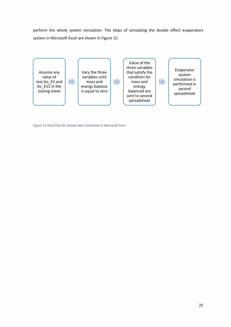
25
perform the whole system simulation. The steps of simulating the double effect evaporators
system in Microsoft Excel are shown in Figure 15.
Figure 15 Data flow for steady-state simulation in Microsoft Excel
Assume any value of
mst,Xo_EV and Xo_EV2 in the testing sheet
Vary the three variables until
mass and energy balance is equal to zero
Value of the three variables that satisfy the condition for
mass and energy
balanced are sent to second
spreadsheet
Evaporator system
simulation is performed in
second spreadsheet

26
Figure 16 Testing sheet for double effect evaporator

27
In the second spreadsheet or the steady-state simulation spreadsheet, all the equations
originated from the ACM examples will be calculated but in sequential modular operation. All the
equations explained in the chapter will be set in the selected cell. As an example, Eq. (1) in
Chapter 4 is applied to calculate the pressure of the steam in the boiler correlate to the
temperature of the steam. Figure 18 shows how the equation is employed to the Microsoft Excel.
Figure 17 Steady-state simulation spreadsheet for double effect evaporator in Microsoft Excel
Figure 18 Equation is applied for steady-state simulation in the Microsoft Excel
5.1.4 Investigation of Steady-state Model in Matlab
The same working principle in the Microsoft Excel is applied for the steady-state simulation model
in Matlab. The steady-state simulation model in Matlab, as shown in red circle Figure 19 still uses
the three variables to influence equation of the mass and energy balance such in the testing sheet

28
in Microsoft Excel simulation. Again, the objective is to equal Eq. (6) and (8) to zero. The three
main variables will continuously be varied until the objective is achieved. Meanwhile in Matlab,
the steady-state simulation is done in a single window, unlike in Microsoft Excel whereby two
spreadsheets are used and connected to each other. All the equations are set in the single
interphase, and each calculated result from the equations are stored in the workspace presented
in the dotted line in Figure 19. Only the energy balance calculation of the evaporator as shown in
the green circle in Figure 19 and the value of the three variables will be shown in the command
window section. Unlike in Microsoft Excel, for the normal calculation Matlab operation, the
arrangement of the equation is more vital. Mis-arrangement of equations can lead to failure of
simulating the model where some of the equations variable are related.
Figure 19 Steady-state simulation in Matlab
5.1.5 Investigation of Optimisation Model in ACM
Besides the steady-state run, the ACM also provides an optimisation simulation run. Eq. (13) to
Eq. (17) in section 4.3 is the set of costing equations taken from the ACM example. These
equations are constructed to optimise the evaporation process in the simulation, and the way of
these equations written in the ACM is shown in Figure 20. The equations are believed to be a
unique formula to calculate the cost of running an evaporator plant. Hence, the objective
function in this optimisation simulation is to minimise the overall cost that represented by Eq.
(18) by manipulating the value of all the variables involved in Eq. (13) to Eq. (17).

29
Figure 20 Optimisation equations for double evaporators
For the example in ACM, three decision variables are chosen as Figure 21 shown to manipulate
the value of the variables used in the costing equations. The three decision variables are the
liquid valve coefficient, the steam valve coefficient, and pressure of the steam that is produced
from the second evaporator. Optimisation tool in the ACM will help to calculate the best value of
these decision variables, thus optimise the objective function value
Figure 21 Three variables that manipulated for optimisation test run
However, the decision variables that have been chosen are only used for the example and can be
changed if a new condition or finding is present. Appendix E provides the steps to apply the new
decision variables as well as the constraints.

30
5.1.6 Investigation of FSolve Model in Matlab
The ‘FSolve’ function is one of the features provided by Matlab. This feature is suitable to use in
solving an equation that has the objective to achieve the value of zero. This tool will calculate the
optimum value of selected variable until the objective is achieved. Unfortunately, no constraint
can be applied to each selected variable in using the ‘FSolve’ tool compared to the ACM
optimisation tool. In some cases, the variables chosen can exceed the limit that has been fixed
earlier (Attaway 2013). ‘Fmincon’ is not chosen to be the optimisation Matlab tool because to
implement a big number of constraint for each variables, a good constraint equation is required.
Due to some time and capability constraints in designing the constraint equations, ‘FSolve’ is the
best option to replace the ’Fmincon’.
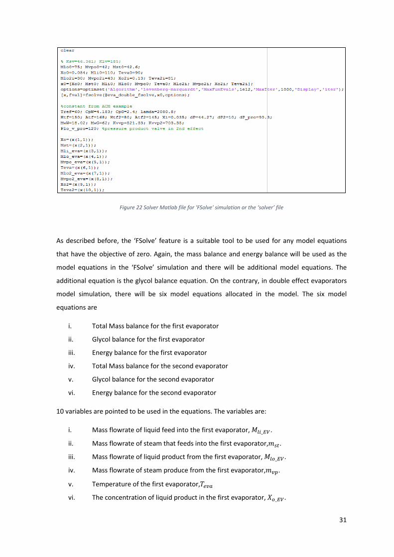
To create a steady-state simulation run by ‘FSolve’, two Matlab files need to be prepared. The
first file is where all the initial conditions are set. This first file is called as the ‘solver’ file and the
second file is called as the ‘main’ file. ‘Main’ file is where all the variables and model equations
are defined. Figure 22 and Figure 23 show the example of ‘main’ and ‘solver’ file used for
simulation in ‘FSolve’. Besides setting the initial conditions, in ‘solver’ file, the user can choose the
solver algorithm. ‘Levenberg-Marquardt’ algorithm is recommended by the Matlab itself to be
used in this simulation. Also, the ‘solver’ file for single and multiple effect evaporators simulation
is standardised with the same type of algorithm and the same amount of function evaluation. The
maximum number of iteration is varied based on the number of the objective function. The
higher number of model equations set in the ‘main’ file, the higher the number of iterations
needed for the ‘solver’ to solve the ‘main’ file.
While running this simulation model, ‘Fsolve’ function in the solver files will recognise all the
model equations in the ‘main’ file objective. Here are the optimum values of each variable so that
the model equations introduced can achieve the value of zero is calculated by the ‘FSolve’ tool.
31
Figure 22 Solver Matlab file for 'FSolve' simulation or the ‘solver’ file
As described before, the ‘FSolve’ feature is a suitable tool to be used for any model equations
that have the objective of zero. Again, the mass balance and energy balance will be used as the
model equations in the ‘FSolve’ simulation and there will be additional model equations. The
additional equation is the glycol balance equation. On the contrary, in double effect evaporators
model simulation, there will be six model equations allocated in the model. The six model
equations are
i. Total Mass balance for the first evaporator
ii. Glycol balance for the first evaporator
iii. Energy balance for the first evaporator
iv. Total Mass balance for the second evaporator
v. Glycol balance for the second evaporator
vi. Energy balance for the second evaporator
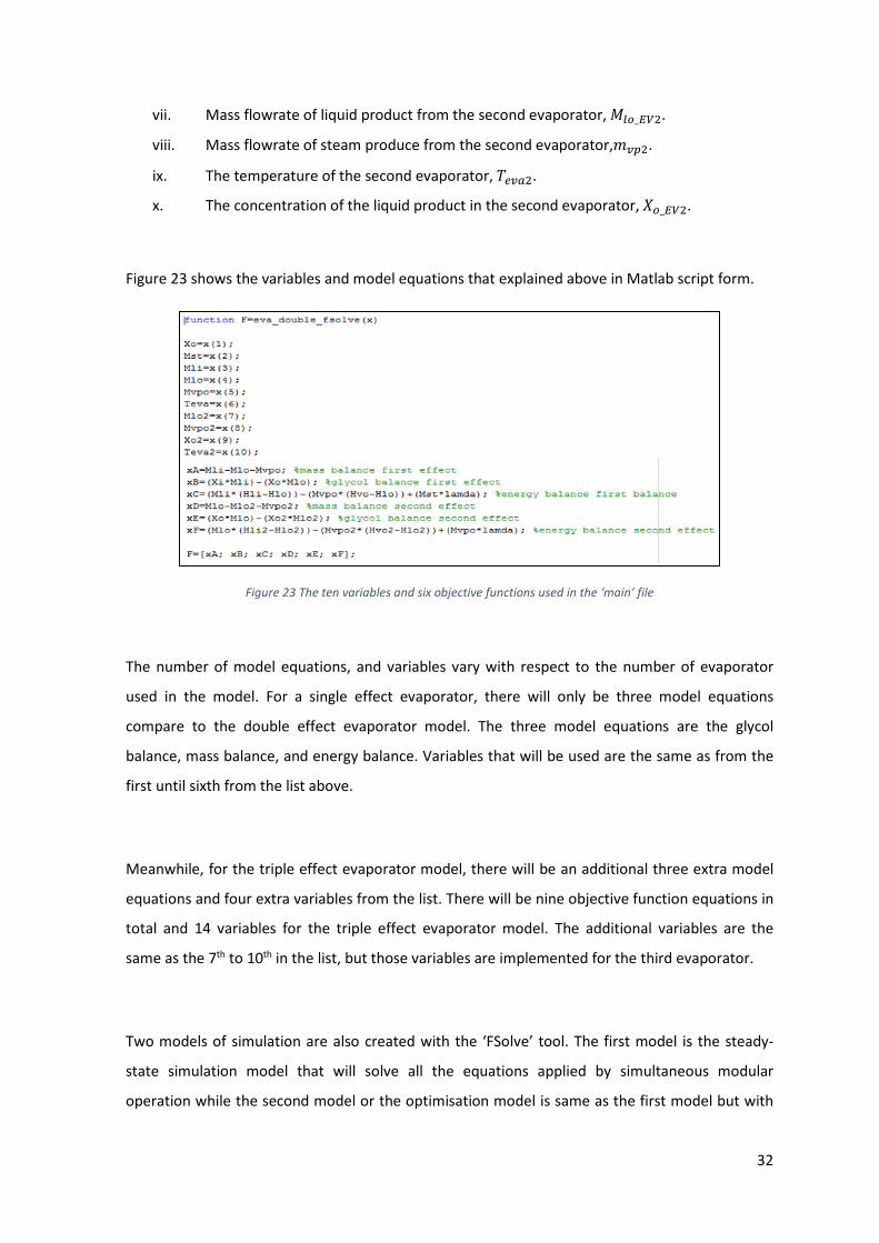
10 variables are pointed to be used in the equations. The variables are:
i. Mass flowrate of liquid feed into the first evaporator, 𝑀𝑀𝑙𝑙𝑠𝑠_𝐸𝐸𝐸𝐸.
ii. Mass flowrate of steam that feeds into the first evaporator,𝑚𝑚𝑠𝑠𝑠𝑠.
iii. Mass flowrate of liquid product from the first evaporator, 𝑀𝑀𝑙𝑙𝑠𝑠_𝐸𝐸𝐸𝐸.
iv. Mass flowrate of steam produce from the first evaporator,𝑚𝑚𝑙𝑙𝑣𝑣.
v. Temperature of the first evaporator,𝑇𝑇𝑟𝑟𝑙𝑙𝑒𝑒
vi. The concentration of liquid product in the first evaporator, 𝑋𝑋𝑠𝑠_𝐸𝐸𝐸𝐸.
32
vii. Mass flowrate of liquid product from the second evaporator, 𝑀𝑀𝑙𝑙𝑠𝑠_𝐸𝐸𝐸𝐸2.
viii. Mass flowrate of steam produce from the second evaporator,𝑚𝑚𝑙𝑙𝑣𝑣2.
ix. The temperature of the second evaporator, 𝑇𝑇𝑟𝑟𝑙𝑙𝑒𝑒2.
x. The concentration of the liquid product in the second evaporator, 𝑋𝑋𝑠𝑠_𝐸𝐸𝐸𝐸2.
Figure 23 shows the variables and model equations that explained above in Matlab script form.
Figure 23 The ten variables and six objective functions used in the ‘main’ file
The number of model equations, and variables vary with respect to the number of evaporator
used in the model. For a single effect evaporator, there will only be three model equations
compare to the double effect evaporator model. The three model equations are the glycol
balance, mass balance, and energy balance. Variables that will be used are the same as from the
first until sixth from the list above.
Meanwhile, for the triple effect evaporator model, there will be an additional three extra model
equations and four extra variables from the list. There will be nine objective function equations in
total and 14 variables for the triple effect evaporator model. The additional variables are the
same as the 7th to 10th in the list, but those variables are implemented for the third evaporator.
Two models of simulation are also created with the ‘FSolve’ tool. The first model is the steady-
state simulation model that will solve all the equations applied by simultaneous modular
operation while the second model or the optimisation model is same as the first model but with

33
the employment of the same costing equations used in the ACM example. For that reason, there
will be an extra model equation in the ‘main’ file for every optimisation simulation in each
evaporator system. The extra objective function is the Eq. (18), and the method of these costing
equations applied in the optimisation simulation by ‘FSolve’ is provided in Figure 24. The
equations are similar to the ACM example. All the Matlab script of the ‘main’ and ‘solver’ file for
each evaporator can be referred in Appendix F.
The purpose of designing two models is to analyse the performance of simultaneous modular
operation in Matlab and compare with ACM.
Figure 24 Costing equation applied in the 'main' file
5.2 Tabulating and Data Comparison
The result of each software packages is tabulated as in Figure 25 below. The color coding is used
to differentiate the type of simulation. Green is indicating the steady-state simulation, yellow is

34
the color chosen for the optimisation simulation by using ACM, red column indicates the steady-
state simulation by ‘FSolve’, and the last color is grey, designates the simulation by ‘FSolve’ with
costing constraint equations. The implementation of color coding makes the comparison job
more manageable. Further details of this table are attached in Appendix B.
Figure 25 Method of tabulating result of each simulation for triple effect evaporator system
Besides the colour coding, the table also practices the comparison job by using a row separator
for a different evaporator. Figure 25 is the example of a table of results for a triple effect
evaporator simulation. Each evaporator result is separated by using a colour row. As shown in
Figure 25, the blue row separates the value received from the first evaporator and second
evaporator while the green row separate the second and third evaporator value.
With the combination of the colour coding and row separator, the user could differentiate the
result from each simulation and type of evaporator system used for simulation.

35
6.0 Results
Each model that is built in ACM, Microsoft Excel and Matlab will go through several simulations
run and the sequence of the test as shown in Figure 26 below
Figure 26 Flow of simulation test in every software
Based on the flowchart, each model in each software package will start with a steady-state. The
result from the three steady-state simulations is tabulated and compared.
Next, the steady-state model will go through an optimisation simulation. The optimisation
simulation will be done in ACM at first to get the value of liquid valve coefficient,
𝐾𝐾𝑙𝑙𝑙𝑙, steam valve coefficient, 𝐾𝐾𝑠𝑠𝑙𝑙 and pressure of steam out of the evaporator, 𝑃𝑃𝑙𝑙𝑣𝑣_𝐸𝐸𝐸𝐸2. These
three variables have been explained in section 5.1.5. With the new values 𝐾𝐾𝑙𝑙𝑙𝑙, 𝐾𝐾𝑠𝑠𝑙𝑙 and 𝑃𝑃𝑙𝑙𝑣𝑣_𝐸𝐸𝐸𝐸2,
evaporator model simulation in Microsoft Excel and Matlab will perform the optimisation
Steady state simulation in ACM
Steady state simulation in Microsoft Excel
Steady state simulation in Matlab
Optimisation simulation in ACM
Optimisation simulation in Microsoft Excel
Optimisation simulation in Matlab
Steady state simulation by 'FSolve' function in
Matlab
Steady state simulation by using 'FSolve'
simulation values in ACM, Microsoft Excel &
Matlab
Optimisation by 'FSolve' function with costing equations in Matlab
Optimisation by using 'FSolve' with costing equations simulation
values in ACM, Microsoft Excel & Matlab
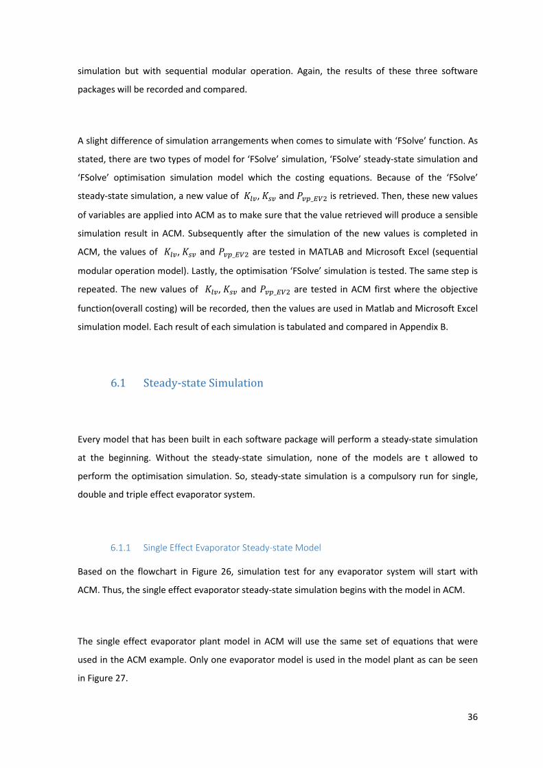
36
simulation but with sequential modular operation. Again, the results of these three software
packages will be recorded and compared.
A slight difference of simulation arrangements when comes to simulate with ‘FSolve’ function. As
stated, there are two types of model for ‘FSolve’ simulation, ‘FSolve’ steady-state simulation and
‘FSolve’ optimisation simulation model which the costing equations. Because of the ‘FSolve’
steady-state simulation, a new value of 𝐾𝐾𝑙𝑙𝑙𝑙, 𝐾𝐾𝑠𝑠𝑙𝑙 and 𝑃𝑃𝑙𝑙𝑣𝑣_𝐸𝐸𝐸𝐸2 is retrieved. Then, these new values
of variables are applied into ACM as to make sure that the value retrieved will produce a sensible
simulation result in ACM. Subsequently after the simulation of the new values is completed in
ACM, the values of 𝐾𝐾𝑙𝑙𝑙𝑙, 𝐾𝐾𝑠𝑠𝑙𝑙 and 𝑃𝑃𝑙𝑙𝑣𝑣_𝐸𝐸𝐸𝐸2 are tested in MATLAB and Microsoft Excel (sequential
modular operation model). Lastly, the optimisation ‘FSolve’ simulation is tested. The same step is
repeated. The new values of 𝐾𝐾𝑙𝑙𝑙𝑙, 𝐾𝐾𝑠𝑠𝑙𝑙 and 𝑃𝑃𝑙𝑙𝑣𝑣_𝐸𝐸𝐸𝐸2 are tested in ACM first where the objective
function(overall costing) will be recorded, then the values are used in Matlab and Microsoft Excel
simulation model. Each result of each simulation is tabulated and compared in Appendix B.
6.1 Steady-state Simulation
Every model that has been built in each software package will perform a steady-state simulation
at the beginning. Without the steady-state simulation, none of the models are t allowed to
perform the optimisation simulation. So, steady-state simulation is a compulsory run for single,
double and triple effect evaporator system.
6.1.1 Single Effect Evaporator Steady-state Model
Based on the flowchart in Figure 26, simulation test for any evaporator system will start with
ACM. Thus, the single effect evaporator steady-state simulation begins with the model in ACM.
The single effect evaporator plant model in ACM will use the same set of equations that were
used in the ACM example. Only one evaporator model is used in the model plant as can be seen
in Figure 27.
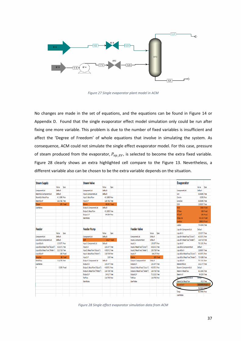
37
Figure 27 Single evaporator plant model in ACM
No changes are made in the set of equations, and the equations can be found in Figure 14 or
Appendix D. Found that the single evaporator effect model simulation only could be run after
fixing one more variable. This problem is due to the number of fixed variables is insufficient and
affect the ‘Degree of Freedom’ of whole equations that involve in simulating the system. As
consequence, ACM could not simulate the single effect evaporator model. For this case, pressure
of steam produced from the evaporator, 𝑃𝑃𝑙𝑙𝑣𝑣_𝐸𝐸𝐸𝐸, is selected to become the extra fixed variable.
Figure 28 clearly shows an extra highlighted cell compare to the Figure 13. Nevertheless, a
different variable also can be chosen to be the extra variable depends on the situation.
Figure 28 Single effect evaporator simulation data from ACM

38
Figure 29 shows the result for steady-state simulation of single effect evaporator in every
software packages used in this research. The table shows that the result difference between the
software is between ±0.0001-0.001%. A solid explanation of this difference is the value that has
been set for the three main elements before the overall simulation start. Each software uses a
slightly dissimilar value and leads to somewhat different results to the simulation. However, the
difference value is still considerable, and the overall simulation in Microsoft Excel and MATLAB
are still valid.
Figure 29 Result for steady-state simulation of single effect evaporator
The steady-state simulation continues with the simulation by ‘FSolve’ function. To speak of the
full version script of the ‘FSolve’ model can refer to Appendix F. Figure 30 shows the result from
steady-state simulation by ‘FSolve’. Compare to the ACM steady-state simulation, a slight
difference in result is produced in ‘FSolve’ simulation. In simulating the model in ‘FSolve’, initial
guesses of the variable are needed. Due to this, steady simulation in ACM and ‘FSolve’ has such
difference. Accurate initial guesses could overcome this problem.
To verify the simulation result produced from ‘FSolve’ function, the values of 𝐾𝐾𝑙𝑙𝑙𝑙 and 𝐾𝐾𝑠𝑠𝑙𝑙 from
‘Fsolve’ simulation as circle in Figure 30 are taken and applied into steady-state simulation model
in ACM and Microsoft Excel. By this step, the result of running a steady-state simulation in
‘FSolve’ function, ACM and Microsoft Excel by using new calculated values of 𝐾𝐾𝑙𝑙𝑙𝑙 and 𝐾𝐾𝑠𝑠𝑙𝑙 from

39
‘FSolve’ function as provided in Figure 30 are compared. Only ±0.0001% error produce between
simulation in Microsoft Excel and ‘FSolve’ while ±0.01% of error between ‘FSolve’ and ACM.
Solver performance might be the reason of the ±0.01% difference between ‘FSolve’ and ACM.
The step is repeated in other evaporator system simulation by using ‘FSolve’.
Figure 30 Steady-state 'FSolve' simulation result comparison for single effect evaporator
6.1.2 Double Effect Evaporator Steady-state Model
For double effect evaporator system, simulation results from Microsoft Excel and Matlab are
essential as the results from both models indicate the performance of the model in each
software. Performance of the models is compared with ACM by tabulating a few variables that
produce from Microsoft Excel and Matlab

40
Result comparison between software packages are presented in Figure 31 and shows there is only
±0.0001-0.001%difference between the software. The results proved positively that model in
Matlab (sequential method) and Microsoft Excel could simulate the steady-state simulation of a
double effect evaporator plant. This means that, without the ACM software, a steady-state
simulation for a double effect evaporator system can be performed and investigation can be
made through the simulation.
Figure 31 Table of result of each simulation for double effect evaporator
Double effect evaporators steady-state simulation continues the ‘FSolve’ simulation. After the
model is developed, the model is tested and the results produced is as shown in Figure 32. As
seen in Figure 32, results produced ±0.01% of error between steady-state simulation by ‘FSolve’
and ACM as well as in Microsoft Excel. This occurrence can be explained by the liquid and steam
valve coefficient value𝐶𝐶 𝐾𝐾𝑙𝑙𝑙𝑙 and 𝐾𝐾𝑠𝑠𝑙𝑙, which are explained in section 6.1.1. However, the model
can be used for learning purposes. Most of the controller learning module is based on Matlab,
thus with this model, student who is taking ‘Instrumentation & Control’ course could learn the
‘FSolve’ model working principle and the method used by the ‘FSolve’ feature to solve the glycol,
total mass and energy balances in the evaporator system.

41
Figure 32 Double effect evaporator ‘FSolve' steady-state simulation result in comparison for different software packages
6.1.3 Triple Effect Evaporator Steady-state Model
The number of equations used in the Microsoft Excel and Matlab models correlates to the
number of evaporators and components existing in the plant. In the triple effect evaporator plant,
more set of equations and components model are used than in the double and single evaporator
plant as seen in Figure 33.
Figure 33 Triple effect evaporator model in ACM

42
Whereas in Microsoft Excel, in ‘testing sheet’ spreadsheet, there is an extra set of total mass and
energy balance applied as shown in Figure 34. With the extra energy and mass balance
calculation, means there is an extra set of equations used in the simulation ‘spreadsheet’ which
can be seen in Figure 34. Further details on the model implementation of triple effect evaporator
simulation in Microsoft Excel and Matlab are given in Appendix C and F respectively.

43
Figure 34 Triple effect evaporator 'testing sheet' in Microsoft Excel model

44
Figure 35 Triple effect evaporator model in Matlab
Whenever there are additional items introduced in the Microsoft Excel, Matlab will also have the
extra piece because both Matlab and Microsoft Excel use the same working principle. Circle items
in Figure 35 are proof of these additional items. The presence of an extra result of energy balance
calculation and concentration product can be seen in Figure 35. The result produced from each
software is presented in Figure 36.

45
Figure 36 Triple effect evaporator steady-state simulation result in every software
Once again, the result produced in each software does not have a significant difference ±0.0001-
0.001% of error will not give a significant influence on the whole simulation. This means steady-
state simulation for triple effect evaporators in Matlab and Microsoft Excel can be used for
investigation or experimentation purposes if the ACM software is not available. But, at first, the
steady-state simulation for triple effect evaporator with the ‘FSolve’ tool shows a ± 1-3%
compared with the result produced by the ACM steady-state simulation difference shown in
Figure 39.

46
This situation occurs due to the initial guesses in ‘FSolve’ solver file. the user is recommended to
use the respected variable value and calculation produced by the ACM or Microsoft Excel for the
initial guesses in the ‘FSolve’ simulation. With this method applied, new values of 𝐾𝐾𝑙𝑙𝑙𝑙 and 𝐾𝐾𝑠𝑠𝑙𝑙 are
produced and the values are applied back into ACM and Microsoft Excel. With these 𝐾𝐾𝑙𝑙𝑙𝑙 and
𝐾𝐾𝑠𝑠𝑙𝑙 new values, the triple effect evaporator simulation in ‘FSolve’ produces a more accurate
result as provided in Figure 37. error between the ‘FSolve’ and ACM simulation has dropped to
±0.0001-0.001%.
Figure 37 Triple effect evaporator ‘FSolve' steady-state simulation result in comparison for different software packages

47
6.2 Optimisation Simulation
The flowchart in Figure 26 states that after the model of steady-state for every software is tested,
construction model of optimisation for every plant in every software begins. Construction of
every model will start with the optimisation model in ACM. Then, this model will be tested. The
technique used for constructing the optimisation model for single and triple effect evaporator in
ACM is similar to the method explained in Section 5.1.5.
Once the model can be run entirely, the 𝐾𝐾𝑙𝑙𝑙𝑙 and 𝐾𝐾𝑠𝑠𝑙𝑙 will be taken and used in Microsoft Excel and
Matlab. The optimisation simulation in Matlab and Microsoft Excel is using the same model that
has been used for the steady-state simulation. Just the value of 𝐾𝐾𝑙𝑙𝑙𝑙 and 𝐾𝐾𝑠𝑠𝑙𝑙 is changed and uses
the amount that is taken from the ACM. The same steps are repeated for the other systems. The
difference between the plants is the number of costing equations applied in the optimisation
simulation.
Back to Section 5.1.6, optimisation simulation by the ‘FSolve’ will go through a different step. The
optimisation simulation will begin from the ‘FSolve’, and the calculated value for 𝐾𝐾𝑙𝑙𝑙𝑙 and 𝐾𝐾𝑠𝑠𝑙𝑙 will
be used back in ACM. The purpose of doing this step is to analyse the value of objective function
(overall costing) in the ACM by using the value of 𝐾𝐾𝑙𝑙𝑙𝑙 and 𝐾𝐾𝑠𝑠𝑙𝑙 calculated from ‘FSolve’ and
compare the result with optimisation simulation on ACM. After the model can be run entirely,
then those values will be used in Microsoft Excel and Matlab (sequential modular model). The
same process is repeated for each system.
6.2.1 Single Effect Evaporator Optimisation Model
The construction of optimisation model starts with the single effect evaporator plant. Same
arrangement and components are used in the plant model as in Figure 27. At this moment, the
costing equations are applied to the plant, and the costing equations applied in this system are
shown in Figure 38. All the constraint explained in the section 5.1.5 is being applied back into the
single effect evaporator plant.

48
Figure 38 Single effect evaporator optimisation costing equations
The number of the evaporator affects the equations used in the optimisation model for each
plant. With all the constraints and costing equations set up, the single effect evaporator model is
tested to simulate an optimisation simulation. Interestingly, the ACM successfully simulates the
plant model with the optimisation simulation. The result of the optimisation simulation is
presented in Figure 39, and the value for liquid and steam valve, 𝐾𝐾𝑙𝑙𝑙𝑙 and 𝐾𝐾𝑠𝑠𝑙𝑙, are used in Matlab
and Microsoft Excel model. Calculation of the result produced from Matlab and Microsoft Excel
only shows a ±0.0001-0.001% difference from the ACM calculation.
Figure 39 Optimisation simulation result in ACM for single effect evaporator plant
At this stage, ‘FSolve’ with costing equations will be tested first in Matlab. The Matlab script of
this model can be referred in Appendix F. If the model runs as planned, the calculation of 𝐾𝐾𝑙𝑙𝑙𝑙 and
𝐾𝐾𝑠𝑠𝑙𝑙 from the model will be used in ACM. If ACM can simulate the triple effect model by using

49
value 𝐾𝐾𝑙𝑙𝑙𝑙 and 𝐾𝐾𝑠𝑠𝑙𝑙 from ‘FSolve’ optimisation model with a sensible result, then these values will
be tested in Microsoft Excel and Matlab (sequential model). Result of the test is given in Figure
40.
Figure 40 'FSolve' with costing equations simulation result for single effect evaporator
From the result, ± 1-5% of difference produces between the optimisation simulation in ‘FSolve’
and ACM. A bigger difference could be seen in the multiple effect evaporator plant. Explanation
of this problem is again due to the fixed initial guesses define in ‘Fsolve’ solver file. These guesses
could be not too accurate as compared with the ACM optimisation. However, guesses are used to
find the final value in the ‘FSolve’ solver file which is to calculate all the variables including 𝐾𝐾𝑙𝑙𝑙𝑙
and 𝐾𝐾𝑠𝑠𝑙𝑙. Next, the calculated values of 𝐾𝐾𝑙𝑙𝑙𝑙 and 𝐾𝐾𝑠𝑠𝑙𝑙 from the ‘FSolve’ calculations are tested in
ACM. Here, a better result is produced and if the ACM could simulate successfully, the same value
of 𝐾𝐾𝑙𝑙𝑙𝑙 and 𝐾𝐾𝑠𝑠𝑙𝑙 are recycled in Microsoft Excel and Matlab (sequential modular operation).
6.2.2 Double Effect Evaporator Optimisation Model
The step remains the same for double effect evaporator. Plus, in Chapter 5, double effect
evaporator is used as the model example. All the steps to build optimisation for double effect
evaporator either in ACM or ‘FSolve’ optimisation simulation has been explained in Section 5.1.5
and 5.1.6.
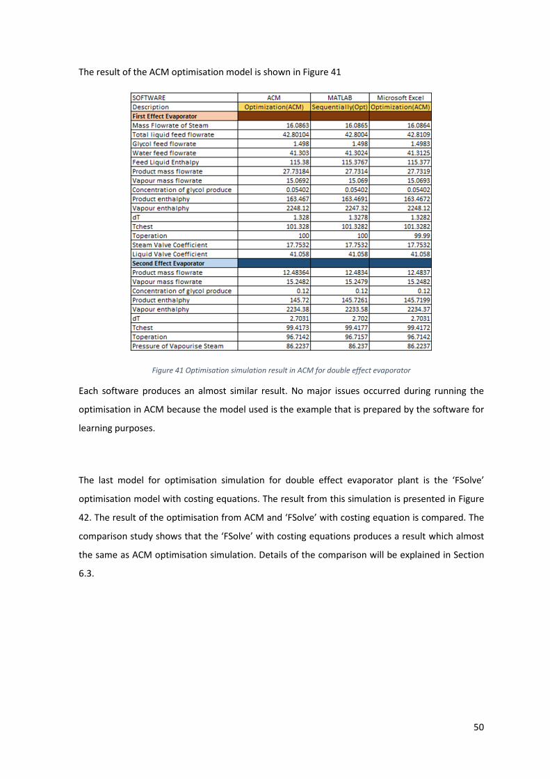
50
The result of the ACM optimisation model is shown in Figure 41
Figure 41 Optimisation simulation result in ACM for double effect evaporator
Each software produces an almost similar result. No major issues occurred during running the
optimisation in ACM because the model used is the example that is prepared by the software for
learning purposes.
The last model for optimisation simulation for double effect evaporator plant is the ‘FSolve’
optimisation model with costing equations. The result from this simulation is presented in Figure
42. The result of the optimisation from ACM and ‘FSolve’ with costing equation is compared. The
comparison study shows that the ‘FSolve’ with costing equations produces a result which almost
the same as ACM optimisation simulation. Details of the comparison will be explained in Section
6.3.

51
Figure 42 'FSolve' with costing equations simulation result for double effect evaporator
6.2.3 Triple Effect Evaporator Optimisation Model
Refer to Figure 33. The same arrangements and components are used in the optimisation
simulation. There are new costing equations introduced in the optimisation model compared to
the double effect evaporator. The new equations are shown in Figure 43. As repeatedly explained
before, the number of the costing equations is related to the amount of the evaporator used in
the plant.

52
Figure 43 Triple effect evaporator optimisation costing equations
The optimisation model in ACM is tested after all the constraints are fixed. The model gives out a
result as shown in Figure 44. Impressively, the triple effect evaporator with optimisation model
ran as planned and produced 82.09% glycol concentration. Although the concentration product
generated is too high and might be not suitable to be used in the real world, the result proves
that the new costing equations together with the constraints is working well to simulate and
optimise a triple effect evaporator system.
Figure 44 Optimisation simulation result in ACM for triple effect evaporator

53
The final stage of the optimisation simulation is developing the ‘FSolve’ optimisation model with
the costing equations used in ACM for triple effect evaporator plant. The red highlighted cell in
Figure 45 indicates a slip out of result from Matlab although there is no unusual script occurs in
the ‘FSolve’ main file script. Moreover, similar equations are used in other simulation models, but
the optimisation by using ‘FSolve’ still gives the insensible value. Due to the inaccurate value from
the ‘FSolve’ solver, the value of 𝐾𝐾𝑙𝑙𝑙𝑙 and 𝐾𝐾𝑠𝑠𝑙𝑙 produced is invalid. Hence, a bit of reverse-
engineering method is applied to overcome this problem.
Not all calculations produced from the ‘FSolve’ optimisation simulation are invalid. Part of the
value is still valid and can be used to overcome this problem. The triple effect evaporator plant
model in ACM is used to do the reverse-engineering simulation.
The simulation is done by converting the ‘Fixed value’ of the three variables, which are 𝐾𝐾𝑙𝑙𝑙𝑙, 𝐾𝐾𝑠𝑠𝑙𝑙
and 𝑃𝑃𝑙𝑙𝑣𝑣_𝐸𝐸𝐸𝐸2 into ‘Free value’ (calculated value). Replace the variables with three new ‘fixed value’
and the new ‘Fixed value’ are 𝑋𝑋𝑠𝑠_𝐸𝐸𝐸𝐸, 𝑇𝑇𝐸𝐸𝐸𝐸 and 𝐾𝐾𝑙𝑙𝑙𝑙3. Values for each variable are 0.0953, 100℃, and
10 respectively. ACM would not trace any ‘DOF’ error with the new replacement variables and the
plant model can be simulated. The new simulation will produce new values of 𝐾𝐾𝑙𝑙𝑙𝑙 and 𝐾𝐾𝑠𝑠𝑙𝑙 and
these values are also used in Microsoft Excel and Matlab (sequential modular operation)
simulation. Then, all the initial guesses of value each variable in ‘FSolve’ optimisation simulation
will use from the new simulation value. All these simulations are compared as provided in Figure
45.

54
Figure 45 'FSolve' with costing equations simulation result for triple effect evaporator
Although the initial guess variables in the ‘FSolve’ solver have used value from the ACM
simulation, the same variables are still showing insensible value. Two variables are recognised to
be the source of this problem. The variables are the 𝑇𝑇𝐸𝐸𝐸𝐸2 and 𝑇𝑇𝐶𝐶ℎ𝑟𝑟𝑠𝑠𝑠𝑠2 of second evaporator. These
variables are affecting the calculation of 𝑃𝑃𝑙𝑙𝑣𝑣_𝐸𝐸𝐸𝐸2 in the ‘FSolve’ optimisation simulation, thus
affecting the calculation the value of 𝐾𝐾𝑙𝑙𝑙𝑙 and 𝐾𝐾𝑠𝑠𝑙𝑙. Huge difference can be seen in Figure 45 and
again the red highlighted cells are not only known as invalid but also the source of the problem.

55
6.3 Performance Run and Sensitive Analysis
The last step in the research is the performance run and sensitive analysis phase. There will be
two performance tests that are analysed at this stage. The first test is the performance
comparison of the optimisation simulation between ACM and ‘FSolve’ with costing equation. The
second test is about analysing the evaporator system performance used in the single, double and
triple effect evaporator plant. The double effect evaporator acts as the reference indicator.
6.3.1 Performance Comparison between ACM Optimisation and ‘FSolve’ with Costing
Constraint
Figure 46 Optimisation objective function comparison of ACM and 'FSolve'
Analysis of this test is done by comparing the results of the objective function. This feature is built
by the ACM to see the changes of the selected variables during optimisation simulation. Hence,
the test begins with running the entire plant model in ACM with a steady-state simulation. After
the steady-state simulation is done, the plant model will go through the optimisation simulation.
The table on the right side in Figure 46 are the results created from optimisation in ACM. Next,

56
the test continues with a steady-state simulation but using the value of 𝐾𝐾𝑙𝑙𝑙𝑙, 𝐾𝐾𝑠𝑠𝑙𝑙 and 𝑃𝑃𝑙𝑙𝑣𝑣_𝐸𝐸𝐸𝐸2 from
the ‘FSolve’ with costing equations model. Outcomes from the usage of the values 𝐾𝐾𝑙𝑙𝑙𝑙, 𝐾𝐾𝑠𝑠𝑙𝑙 and
𝑃𝑃𝑙𝑙𝑣𝑣_𝐸𝐸𝐸𝐸2 is shown in the table on the left side in Figure 46. While for triple effect evaporators
simulation, there is an extra step due to the small miscalculation of variables in ‘FSolve’
optimisation simulation which has been explained in 6.2.3 section.
The calculation of objective function in Figure 46 shows that ACM and ‘FSolve’ optimisation
simulation have an almost similar capability in optimising the single or multiple effect evaporators
system. The result proves that ‘FSolve’ simulation with costing equations can be utilised to
perform optimisation simulation without the presence of ACM except for the triple effect
evaporator. ‘FSolve’ with costing equation simulation for triple effect evaporator need the
occurrence of ACM software to correct the problem that arises.
6.3.2 Sensitive Analysis of the Single and Triple effect evaporator system.
The purpose of doing this analysis is to test the performance of the constructed evaporator
model. The evaporator model that will be tested is single and triple effect evaporator system.
Two tests are created to test their performance. The first test is where 𝑀𝑀𝑙𝑙𝑠𝑠_𝐸𝐸𝐸𝐸 and final glycol
product concentration will be fixed. The amount of mass flowrate of steam in each system to
produce the glycol concentration that has been set at first will be evaluated. While in the second
test, the fixed percentage of glycol concentration is replaced by the mass flowrate of liquid feed
into the first evaporator. In this second test, the objective is to evaluate the three systems by
valuing the glycol concentration in the final product solution. The result of these two tests is
tabulated and compared.
Table 3 First test performance analysis result
Single Effect
Evaporator
Double Effect
Evaporator
Triple Effect
Evaporator
Mass flowrate of liquid feed in (kg/min) 116.993 116.993 116.993

57
As expected in running the first performance analysis, single effect evaporator system will need
the highest amount of flowrate of steam as shown in Table 3 to produce of a 13% of glycol
concentration in the final product solution. The solid reason for this result is in double and triple
effect evaporator system; the feed liquid will go through two or three times of evaporation
process. Means, more water is eliminated from the solution, and the usage of steam is recycled
but not in single effect evaporator. The feed solution only goes through evaporation process
once. Thus, more steam is needed to provide enough energy to eliminate the water in the
solution to produce the final product solution with 13% of glycol concentration.
While doing the first test, an extra analysis is done. The analysis aims to find the limitation of
glycol concentration, which can be produced by a 116.993 kg/min liquid feed into each system.
The analysis is graphed by the concentration of glycol in final product against the flowrate of
steam feed into the system. The graph is as shown in Figure 47. With the graph in Figure 47, each
system shows their cut-off of concentration. The cut-off means, that if a higher amount of mass
flowrate of steam is fed, the system will not produce a higher glycol concentration solution. Single
effect evaporator has a cut-off of glycol concentration at 42.33% while double effect evaporator
at 47.9% glycol concentration and triple effect evaporators system at 99%. Result in the second
test will support the outcome of this extra test. Figure 48 is the continuation of the graph in
Figure 47. Although concentration product in triple effect could achieve 99%, the flowrates of the
final solution produced is small (4.2 kg/min), and that flowrate is not suitable for large-scale
production. The graph in Figure 47 and Figure 48 could be a reference to the performance of the
evaporator system subject to variables that fixed in section 5.1.1.
Mass flowrate of steam feed in (kg/min) 84.8136 42.6525 27.0517
Mass flowrate of liquid produce out
(kg/min)
31.485 31.485 31.485
Glycol concentration in final product 0.130054 0.130054 0.130054
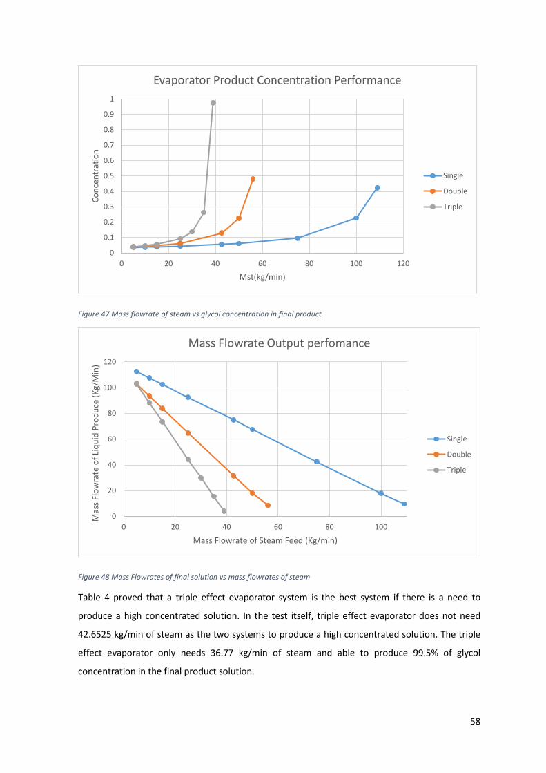
58
Figure 47 Mass flowrate of steam vs glycol concentration in final product
Figure 48 Mass Flowrates of final solution vs mass flowrates of steam
Table 4 proved that a triple effect evaporator system is the best system if there is a need to
produce a high concentrated solution. In the test itself, triple effect evaporator does not need
42.6525 kg/min of steam as the two systems to produce a high concentrated solution. The triple
effect evaporator only needs 36.77 kg/min of steam and able to produce 99.5% of glycol
concentration in the final product solution.
0
0.1
0.2
0.3
0.4
0.5
0.6
0.7
0.8
0.9
1
0 20 40 60 80 100 120
Conc
entr
atio
n
Mst(kg/min)
Evaporator Product Concentration Performance
Single
Double
Triple
0
20
40
60
80
100
120
0 20 40 60 80 100
Mas
s Flo
wra
te o
f Liq
uid
Prod
uce
(Kg/
Min
)
Mass Flowrate of Steam Feed (Kg/min)
Mass Flowrate Output perfomance
Single
Double
Triple

59
However, each system has their own pros and cons depend on the needs and the current
situation. As an example, if in the current situation, the cost in producing steam is not so costly
and the final glycol concentration desire is less than 42%, the single effect evaporator still could
be considered as a suitable system. The reason for this statement is with constructing a single
effect evaporator, more space and maintenance cost can be saved. Plus, running a single effect
evaporator is not as complex as running a double or triple effect evaporator system. The presence
of performance analysis as above will be beneficial to choose the best system to be used based
on the present needs.
Table 4 Second test performance analysis result
Single Effect
Evaporator
Double Effect
Evaporator
Triple Effect
Evaporator
Mass flowrate of liquid feed in (kg/min) 116.993 116.993 116.993
Mass flowrate of steam feed in (kg/min) 42.6525 42.6525 36.77
Mass flowrate of liquid produce out
(kg/min)
72.639 31.4851 4.114
Glycol concentration in final product 0.053671 0.130054 0.995311

60
7.0 Conclusion
In this section, all the achievements and efforts throughout the project are discussed. Aims of the
project will be reviewed as well as the accomplishments of the project are presented.
In Chapter 2, which is the literature review section, the difference between evaporation and
distillation process has been briefly explained. In addition, a few examples of the type of glycol
and a brief explanation on how this glycol is produced in the real industry has also been
presented in this section. Not to forget, the types of the evaporator that occur in the industry and
the software packages used in this project.
ACM, Microsoft Excel, and Matlab are the software packages used to develop the single, double
and triple effect evaporator system. The case study was based on the example of double effect
evaporator system in ACM. Investigation of this case study, a double effect evaporator model for
Microsoft Excel and Matlab (sequential modular), are successfully developed. This model could
not be constructed if the in-depth investigation of each component model in the example from
ACM is not carried out. All the mathematical equations in the steamer, steam valve, feeder, liquid
pump, liquid valve, and evaporator were thoroughly checked and tested in Microsoft Excel. From
here, two spreadsheets are built for all evaporator system. The first spreadsheet is used to test
the energy balance and mass balance, and after the balance calculation is done, the calculations
are carried to the real steady-state simulation.
The Matlab steady-state simulation (sequential modular) of double effect evaporator uses the
same process as in the Microsoft Excel. With all the experiences gained from constructing the
double evaporator system, the knowledge is applied to develop single and triple effect
evaporator. Plus, a steady-state simulation is also successfully developed by using ‘FSolve’ feature
in Matlab. It is proudly presented that all the software packages are successful in running the
steady-state simulation for single, double and triple effect evaporator system.

61
After the steady simulation is done, this project is continued in building the optimisation
simulation. Again, the case study of double effect evaporator from the ACM was taken as an
example, and the optimisation costing equations are studied. The costing equations are applied in
optimising the single and triple effect evaporator system with some modification. The
modification is based on the number of evaporators used. The optimisation simulation was tried
and produced a positive result. During the investigation of the optimisation in ACM, the idea of
implementing the costing equations into the steady-state simulation model of ‘FSolve’ feature in
Matlab appeared. This feature is suitable to use for a model that has a model equation that needs
to achieve the value zero.
The optimisation simulation for each evaporator system is considered as a successful run. The
same achievement is met for the ‘FSolve’ model, but unfortunately, for the triple effect
evaporator system in ‘FSolve’ optimisation has a slight glitch in the result. With the small errors
occurred, the ‘FSolve’ model for triple effect evaporator system could not fully utilise without the
help from the ACM. Thus, the ‘FSolve’ optimisation model of triple effect evaporator could only
be tested along with the presence of ACM. Further investigation is needed to overcome this
problem.
Last but not least, a sensitive analysis was carried out to find the limitation of the single and triple
effect evaporator. Two parameters are used for the single effect evaporator and three
parameters for triple effect evaporators. The analysis concluded that for single effect evaporator,
the minimum and maximum value of 𝐾𝐾𝑙𝑙𝑙𝑙 and 𝐾𝐾𝑠𝑠𝑙𝑙 for the project can be applied and ACM would
simulate without any error but not for triple effect evaporator. Certain parameters of evaporator
will have their own values of minimum and maximum of 𝐾𝐾𝑙𝑙𝑙𝑙 and 𝐾𝐾𝑠𝑠𝑙𝑙 . After deeper investigation
is made, triple effect evaporator has a higher efficient compared to single effect evaporator.
Triple evaporator could produce higher concentration product with lesser mass a flowrate of
liquid fed, the which means it is more economically wise.
This project is a privilege for any researcher who is keen to gain knowledge in exploring the
working principle of simulation in the software packages used and mathematical equation applied
in the different effects of evaporator system.

62
7.1 Future work
This section discusses the possible future work that can be considered by forthcoming students
for this project.
This research has covered the understanding of the mathematical model of single, double, and
triple effect evaporators with the model developed by ASPEN technology. Other than that, this
research also has explained the development of a steady-state model for single to triple
evaporators in ACM, Microsoft Excel, and Matlab. The model includes the optimisation model in
ACM for single, double, and triple effect evaporator as well as their sensitivity analysis. Moreover,
a new type of steady-state model also has been constructed, which is the ‘FSolve’ feature model.
Here are some suggestions that can be made for future work:
1. Using ‘FMinCon’ to run optimisation simulation in Matlab.
2. Build a dynamic simulation of all the systems.
3. Implement a control system into the evaporator systems.

63
Reference
APV. 2008. "Evaporator Handbook." In: SPX Brand. http://www.spxflow.com/en/assets/pdf/Evaporator_Handbook_10003_01_08_2008_US.pdf.
Attaway, Stormy. 2013. "Chapter 1 - Introduction to MATLAB." In Matlab (Third Edition), 3-32. Boston: Butterworth-Heinemann.
Britannica, The Editors of Encyclopedia. Glycol. Encyclopedia Britannica,inc. 2015. Available from https://www.britannica.com/science/glycol.
Dukkipati, Rao V. 2009. "MATLAB: An Introduction with Applications." In. New Dehli, India: New Age International Pvt Ltd Publishers. https://ecedmans.files.wordpress.com/2014/03/matlab-an-introduction-with-applications-rao-v-dukkipati.pdf.
French, Ted. What is Microsoft Excel and What Would I Use it for? ThoughtCo 2016. Available from https://www.thoughtco.com/what-is-microsoft-excel-3573533.
Jr, John J. McKetta. 1984. Ethanol As Fuel: Options: Advantages, And Disadvantages To Exhaust Stacks: Cost. In Encyclopedia Of Chemical Processing And Design: Marcel Dekker,Inc.
Linh T. T. Vu, Parisa A.Bahri, Graeme R.Cole. 2016. Teaching Process System Engineering in Instrumentation & Control and Chemical Engineering Program. In Chemeca, edited by Murdoch University School of Engineering and Information Technology. Adelaide, Australia.
Pabasara. Difference Between Evaporation and Distillation. Pediaa 2017. Available from http://pediaa.com/difference-between-evaporation-and-distillation/.
Patel, Dr. N. K. 2009. Lecture 19: Propylene Gycol. http://nptel.ac.in/courses/103106109/11-20/Lecture%2019%20Propylene%20glycol.pdf.
Ramli, Aida Liyana. 2016. Modelling and Optimising Single And Multiple Effect Evaporators Using Aspen Custom Modeler (ACM), School of Engineering and Information Technology, Murdoch University.

64
Appendix A (Steady-state Result from ACM in Microsoft Excel)
1. Single Effect Evaporator

65
2. Double effect evaporator

66
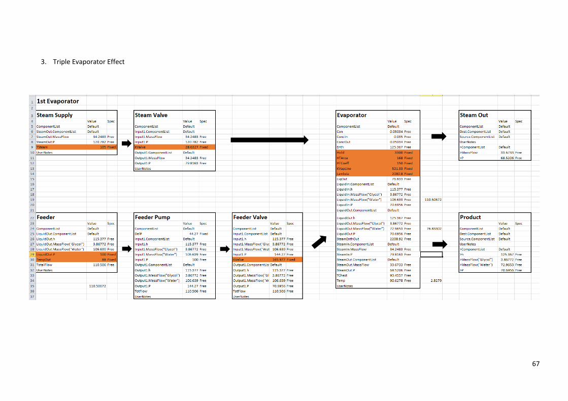
67
3. Triple Evaporator Effect
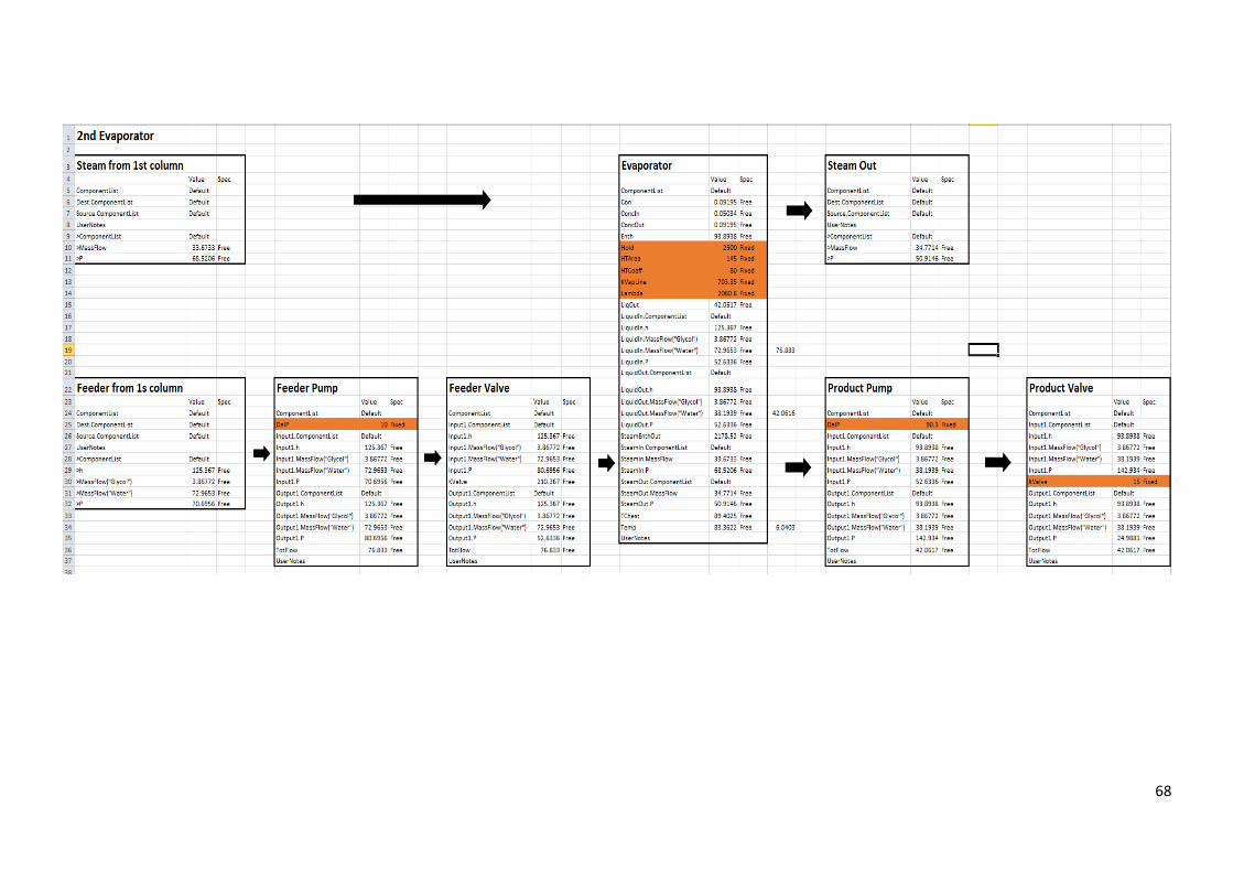
68

69

70
Appendix B (Result Comparison)
1. Single effect evaporator

71
2. Double effect evaporator
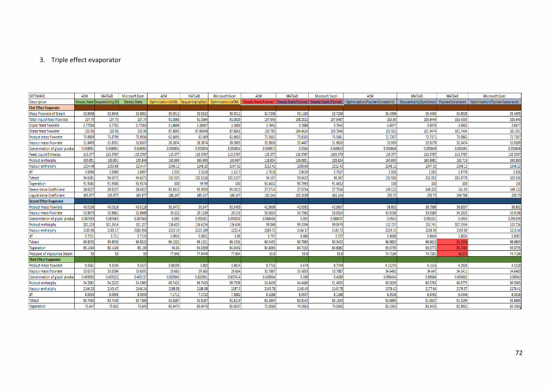
72
3. Triple effect evaporator

73
Appendix C (Microsoft Excel Model)
1. Single effect evaporator
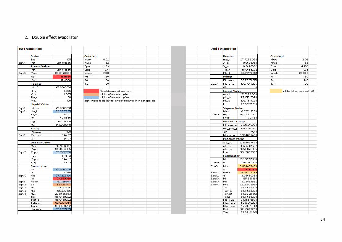
74
2. Double effect evaporator
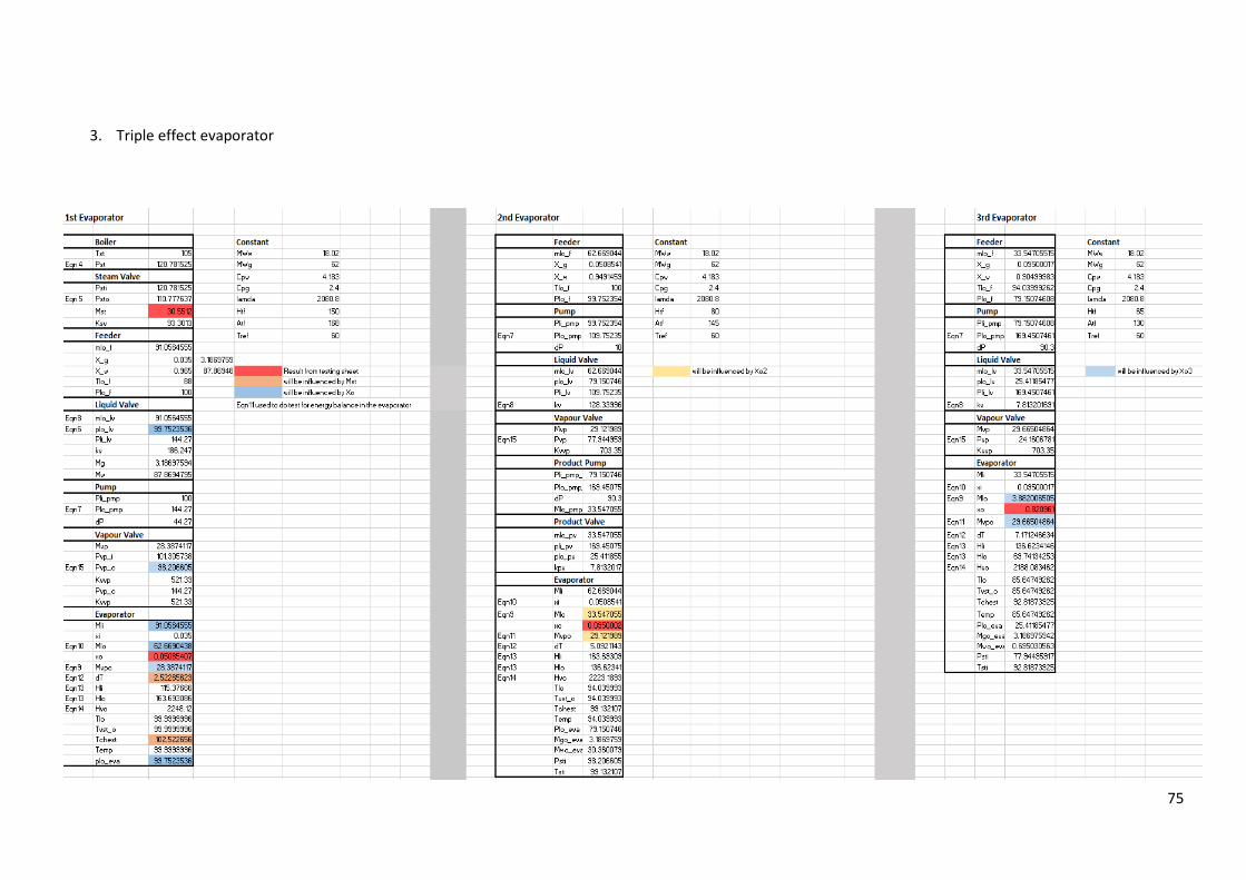
75
3. Triple effect evaporator

76
4. Testing sheet

77

78
Appendix D (ACM equations)
1. Evaporator
2. Pump
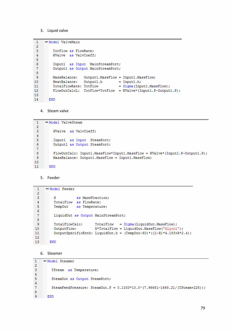
79
3. Liquid valve
4. Steam valve
5. Feeder
6. Steamer

80
7. Single effect evaporator optimisation equations
8. Double effect evaporator optimisation equations
9. Triple effect evaporator optimisation equations
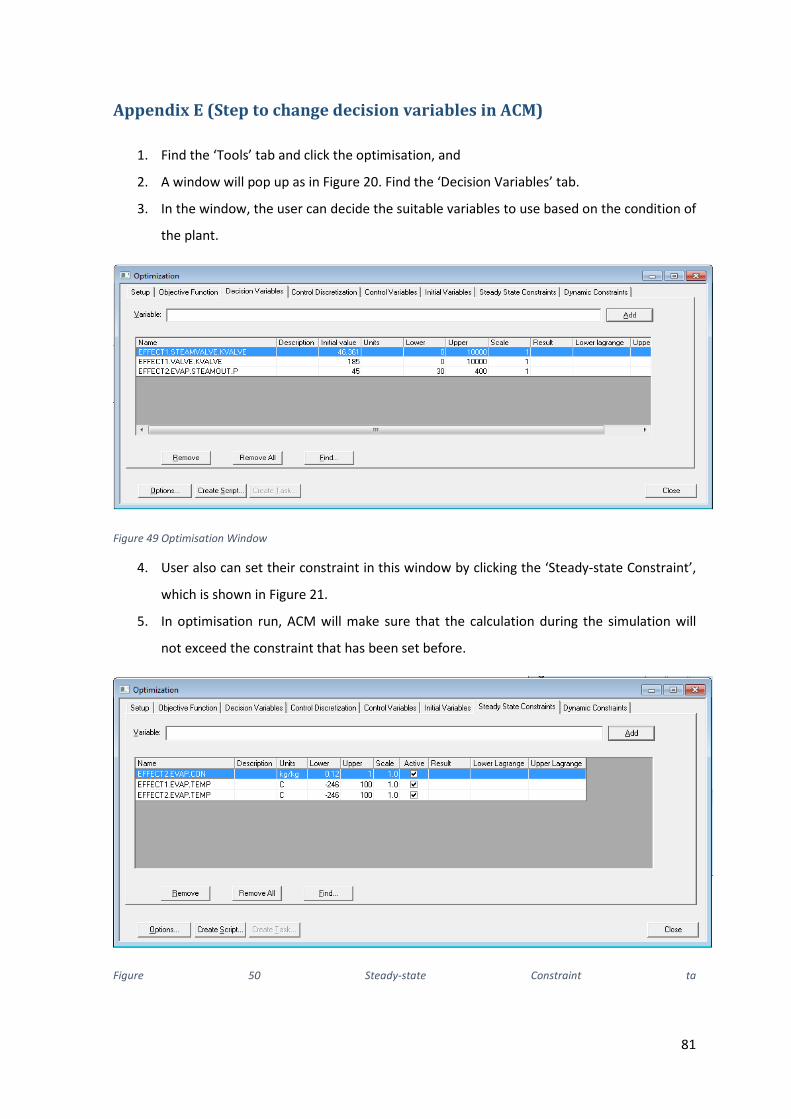
81
Appendix E (Step to change decision variables in ACM)
1. Find the ‘Tools’ tab and click the optimisation, and
2. A window will pop up as in Figure 20. Find the ‘Decision Variables’ tab.
3. In the window, the user can decide the suitable variables to use based on the condition of
the plant.
Figure 49 Optimisation Window
4. User also can set their constraint in this window by clicking the ‘Steady-state Constraint’,
which is shown in Figure 21.
5. In optimisation run, ACM will make sure that the calculation during the simulation will
not exceed the constraint that has been set before.
Figure 50 Steady-state Constraint ta

82
Appendix F (Matlab Script)
1. Single effect steady-state simulation
clear; %% constant for first evaporator x(1)=26.4176; %initial guest of mst x(2)=0.0516023;%initial guest of xo Xf=0.035; %glycol mass fraction from feeder Tst_st=105; %steam temperature from steamer Kvst=60.0553; %steam valve coefficient Tli=88; %temperature of liquid in the feeder Pli=100; %liquid pressure in the feeder Klv=130.5785; %liquid valve coefficient Htf=150; %heat transfer coefficient Atf=168; %heat transfer area lamda=2080; %water latent heat of evaporation at 160C Kvvp=521.33; % steam valve coefficient in the evaporator Cpg=2.4; %specific entalphy of glycol Cpw=4.183; %specific entalphy of water Tref=60; %temperature reference dP=44.27; %pressure created from pump MWw=18.02; %molar mass of water MWg=62; %molar mass of glycol %% 1st effect of evaporator %% Steamer Pst_st=0.1333*10^(7.96681-(1668.21/(Tst_st+228))); Mst= x(1); %% Steam valve Psti_v=Pst_st; Psto_v=Psti_v-((Mst^2)/Kvst); inv1=log10(Psto_v/0.1333); Tsto_v=(1668.21/(7.96681-inv1))-228; %% Feeder Hli=(Tli-Tref)*(((1-Xf)*Cpw)+(Xf*Cpg)); %% Pump Plo_pmp=dP+Pli; %temperature, mass flowrate and entalphy of the liquid from the feeder are not changing. %just the pressure of the liquid changed. %% Main valve Pli_v=Plo_pmp;
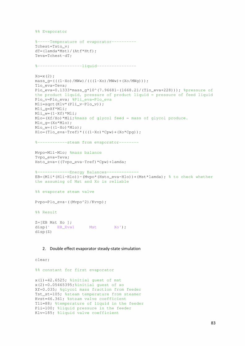
83
%% Evaporator %-----Temperature of evaporator---------- Tchest=Tsto_v; dT=(lamda*Mst)/(Atf*Htf); Teva=Tchest-dT; %------------------liquid---------------- Xo=x(2); mass_g=(((1-Xo)/MWw)/(((1-Xo)/MWw)+(Xo/MWg))); Tlo_eva=Teva; Plo_eva=0.1333*mass_g*10^(7.96681-(1668.21/(Tlo_eva+228))); %pressure of the product liquid, pressure of product liquid = pressure of feed liquid Plo_v=Plo_eva; %Pli_eva=Plo_eva Mli=sqrt(Klv*(Pli_v-Plo_v)); Mli_g=Xf*Mli; Mli_w=(1-Xf)*Mli; Mlo=(Xf/Xo)*Mli;%mass of glycol feed = mass of glycol produce. Mlo_g=(Xo*Mlo); Mlo_w=((1-Xo)*Mlo); Hlo=(Tlo_eva-Tref)*(((1-Xo)*Cpw)+(Xo*Cpg)); %------------steam from evaporator-------- Mvpo=Mli-Mlo; %mass balance Tvpo_eva=Teva; Hsto_eva=((Tvpo_eva-Tref)*Cpw)+lamda; %-------------Energy Balances------------- EB=(Mli*(Hli-Hlo))-(Mvpo*(Hsto_eva-Hlo))+(Mst*lamda); % to check whether the assuming of Mst and Xo is reliable %% evaporate steam valve Pvpo=Plo_eva-((Mvpo^2)/Kvvp); %% Result Z=[EB Mst Xo ]; disp(' EB_Eva1 Mst Xo'); disp(Z)
2. Double effect evaporator steady-state simulation
clear; %% constant for first evaporator x(1)=42.6525; %initial guest of mst x(2)=0.05465395;%initial guest of xo Xf=0.035; %glycol mass fraction from feeder Tst_st=105; %steam temperature from steamer Kvst=46.361; %steam valve coefficient Tli=88; %temperature of liquid in the feeder Pli=100; %liquid pressure in the feeder Klv=185; %liquid valve coefficient

84
Htf=150; %heat transfer coefficient Atf=168; %heat transfer area lamda=2080; %water latent heat of evaporation at 160C Kvvp=521.33; % steam valve coefficient in the evaporator Cpg=2.4; %specific entalphy of glycol Cpw=4.183; %specific entalphy of water Tref=60; %temperature reference dP=44.27; %pressure created from pump MWw=18.02; %molar mass of water MWg=62; %molar mass of glycol %% Constant of 2nd effect evaporator x(3)=0.130058; %initial guest of xo2 Plo2_pv2=120; %Pressure after the product valve Htf2=80; Atf2=145; dP2=10; %'second effect' pressure created from feed pump dP_pp2=90.3; %'second effect' pressure created from product pump Kvvp2=703.35; %'second effect' vapour valve coefficient %% 1st effect of evaporator %% Steamer Pst_st=0.1333*10^(7.96681-(1668.21/(Tst_st+228))); Mst= x(1); %% Steam valve Psti_v=Pst_st; Psto_v=Psti_v-((Mst^2)/Kvst); inv1=log10(Psto_v/0.1333); Tsto_v=(1668.21/(7.96681-inv1))-228; %% Feeder Hli=(Tli-Tref)*(((1-Xf)*Cpw)+(Xf*Cpg)); %% Pump Plo_pmp=dP+Pli; %temperature, mass flowrate and entalphy of the liquid from the feeder are not changing. %just the pressure of the liquid changed. %% Main valve Pli_v=Plo_pmp; %% Evaporator %-----Temperature of evaporator---------- Tchest=Tsto_v; dT=(lamda*Mst)/(Atf*Htf); Teva=Tchest-dT;

85
%------------------liquid---------------- Xo=x(2); mass_g=(((1-Xo)/MWw)/(((1-Xo)/MWw)+(Xo/MWg))); Tlo_eva=Teva; Plo_eva=0.1333*mass_g*10^(7.96681-(1668.21/(Tlo_eva+228))); %pressure of the product liquid, pressure of product liquid = pressure of feed liquid Plo_v=Plo_eva; %Pli_eva=Plo_eva Mli=sqrt(Klv*(Pli_v-Plo_v)); Mli_g=Xf*Mli; Mli_w=(1-Xf)*Mli; Mlo=(Xf/Xo)*Mli;%mass of glycol feed = mass of glycol produce. Mlo_g=(Xo*Mlo); Mlo_w=((1-Xo)*Mlo); Hlo=(Tlo_eva-Tref)*(((1-Xo)*Cpw)+(Xo*Cpg)); %------------steam from evaporator-------- Mvpo=Mli-Mlo; %mass balance Tvpo_eva=Teva; Psto_eva=0.1333*10^(7.96681-(1668.21/(Tvpo_eva+228))); Hsto_eva=((Tvpo_eva-Tref)*Cpw)+lamda; %-------------Energy Balances------------- EB=(Mli*(Hli-Hlo))-(Mvpo*(Hsto_eva-Hlo))+(Mst*lamda); % to check whether the assuming of Mst and Xo is reliable %% evaporate steam valve Pvpo=Plo_eva-((Mvpo^2)/Kvvp); %% 2nd Effect of Evaporator %% Steamer Mst2= Mvpo; Pst2_st=Pvpo; inv2=log10(Pst2_st/0.1333); Tst2_st=(1668.21/(7.96681-inv2))-228; %There is no steam valve between the first column to second column %% Feeder 2 % it comes from first column Mli2=Mlo; Xf2=Xo; Mli2_g=(Mli2*Xf2); Mli2_w=Mli2-Mli2_g; Tli2=Tlo_eva; mass2_g=(((1-Xf2)/MWw)/(((1-Xf2)/MWw)+(Xf2/MWg))); Pli2=0.1333*mass2_g*10^(7.96681-(1668.21/(Tli2+228))); Hli2=(Tli2-Tref)*(((1-Xf2)*Cpw)+(Xf2*Cpg)); %% Pump 2 Plo2_pmp2=Pli2+dP2;
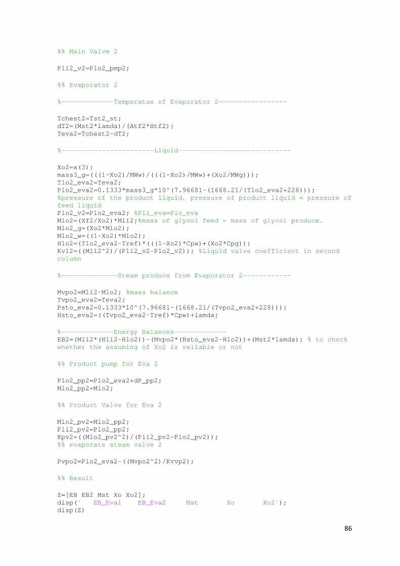
86
%% Main Valve 2 Pli2_v2=Plo2_pmp2; %% Evaporator 2 %-------------Temperatue of Evaporator 2----------------- Tchest2=Tst2_st; dT2=(Mst2*lamda)/(Atf2*Htf2); Teva2=Tchest2-dT2; %-----------------------Liquid---------------------------- Xo2=x(3); mass3_g=(((1-Xo2)/MWw)/(((1-Xo2)/MWw)+(Xo2/MWg))); Tlo2_eva2=Teva2; Plo2_eva2=0.1333*mass3_g*10^(7.96681-(1668.21/(Tlo2_eva2+228))); %pressure of the product liquid, pressure of product liquid = pressure of feed liquid Plo2_v2=Plo2_eva2; %Pli_eva=Plo_eva Mlo2=(Xf2/Xo2)*Mli2;%mass of glycol feed = mass of glycol produce. Mlo2_g=(Xo2*Mlo2); Mlo2_w=((1-Xo2)*Mlo2); Hlo2=(Tlo2_eva2-Tref)*(((1-Xo2)*Cpw)+(Xo2*Cpg)); Kvl2=((Mli2^2)/(Pli2_v2-Plo2_v2)); %Liquid valve coefficient in second column %--------------Steam produce from Evaporator 2------------ Mvpo2=Mli2-Mlo2; %mass balance Tvpo2_eva2=Teva2; Psto_eva2=0.1333*10^(7.96681-(1668.21/(Tvpo2_eva2+228))); Hsto_eva2=((Tvpo2_eva2-Tref)*Cpw)+lamda; %-------------Energy Balances------------- EB2=(Mli2*(Hli2-Hlo2))-(Mvpo2*(Hsto_eva2-Hlo2))+(Mst2*lamda); % to check whether the assuming of Xo2 is reliable or not %% Product pump for Eva 2 Plo2_pp2=Plo2_eva2+dP_pp2; Mlo2_pp2=Mlo2; %% Product Valve for Eva 2 Mlo2_pv2=Mlo2_pp2; Pli2_pv2=Plo2_pp2; Kpv2=((Mlo2_pv2^2)/(Pli2_pv2-Plo2_pv2)); %% evaporate steam valve 2 Pvpo2=Plo2_eva2-((Mvpo2^2)/Kvvp2); %% Result Z=[EB EB2 Mst Xo Xo2]; disp(' EB_Eva1 EB_Eva2 Mst Xo Xo2'); disp(Z)

87
3. Triple effect evaporator steady-state simulation
clear; %% constant for first evaporator x(1)=30.5512; %initial guest of mst x(2)=0.05085419;%initial guest of xo Xf=0.035; %glycol mass fraction from feeder Tst_st=105; %steam temperature from steamer Kvst=93.3013; %steam valve coefficient Tli=88; %temperature of liquid in the feeder Pli=100; %liquid pressure in the feeder Klv=186.247; %liquid valve coefficient Htf=150; %heat transfer coefficient Atf=168; %heat transfer area lamda=2080; %water latent heat of evaporation at 160C Kvvp=521.33; % steam valve coefficient in the evaporator Cpg=2.4; %specific entalphy of glycol Cpw=4.183; %specific entalphy of water Tref=60; %temperature reference dP=44.27; %pressure created from pump MWw=18.02; %molar mass of water MWg=62; %molar mass of glycol %% Constant of 2nd effect evaporator x(3)=0.095001; %initial guest of xo2 Htf2=80; Atf2=145; dP2=10; %'second effect' pressure created from feed pump dP_pp2=90.3; %'second effect' pressure created from product pump Kvvp2=703.35; %'second effect' vapour valve coefficient %% Constant of 3rd effect evaporator x(4)=0.821057; %initial guest of xo2 Htf3=65; Atf3=130; Kvvp3=703.35; %'second effect' vapour valve coefficient %% 1st effect of evaporator %% Steamer Pst_st=0.1333*10^(7.96681-(1668.21/(Tst_st+228))); Mst= x(1); %% Steam valve Psti_v=Pst_st; Psto_v=Psti_v-((Mst^2)/Kvst); inv1=log10(Psto_v/0.1333); Tsto_v=(1668.21/(7.96681-inv1))-228; %% Feeder Hli=(Tli-Tref)*(((1-Xf)*Cpw)+(Xf*Cpg));
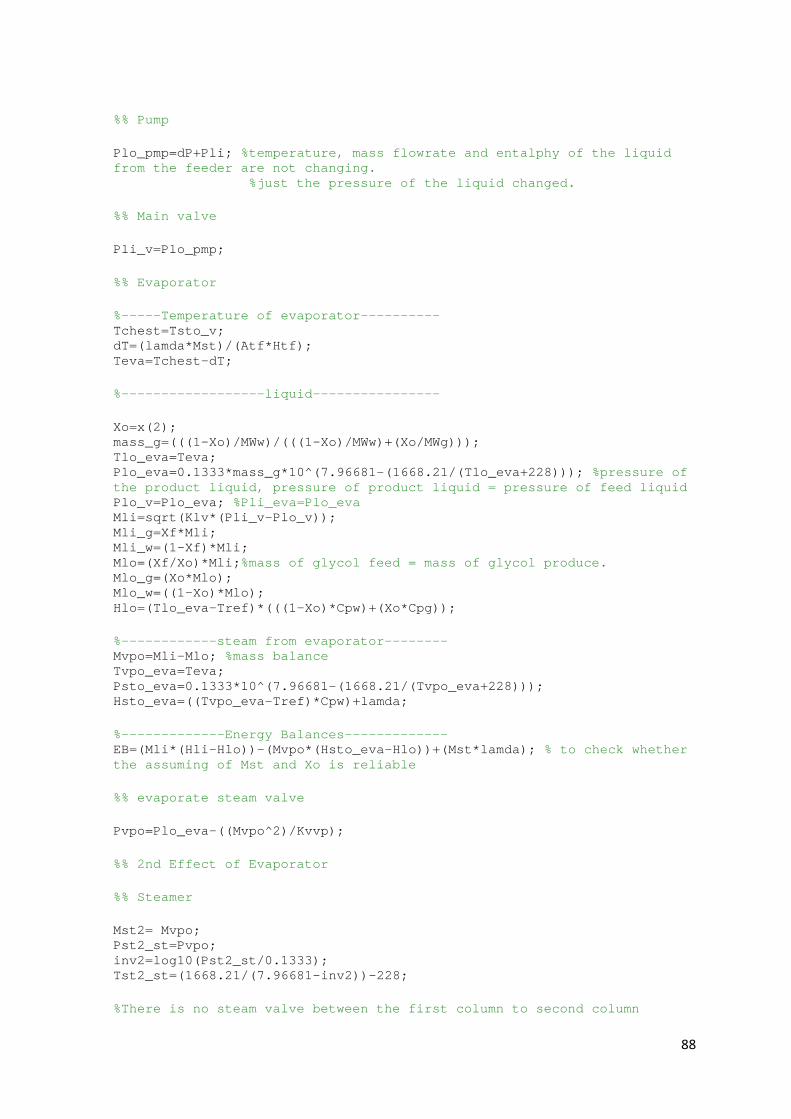
88
%% Pump Plo_pmp=dP+Pli; %temperature, mass flowrate and entalphy of the liquid from the feeder are not changing. %just the pressure of the liquid changed. %% Main valve Pli_v=Plo_pmp; %% Evaporator %-----Temperature of evaporator---------- Tchest=Tsto_v; dT=(lamda*Mst)/(Atf*Htf); Teva=Tchest-dT; %------------------liquid---------------- Xo=x(2); mass_g=(((1-Xo)/MWw)/(((1-Xo)/MWw)+(Xo/MWg))); Tlo_eva=Teva; Plo_eva=0.1333*mass_g*10^(7.96681-(1668.21/(Tlo_eva+228))); %pressure of the product liquid, pressure of product liquid = pressure of feed liquid Plo_v=Plo_eva; %Pli_eva=Plo_eva Mli=sqrt(Klv*(Pli_v-Plo_v)); Mli_g=Xf*Mli; Mli_w=(1-Xf)*Mli; Mlo=(Xf/Xo)*Mli;%mass of glycol feed = mass of glycol produce. Mlo_g=(Xo*Mlo); Mlo_w=((1-Xo)*Mlo); Hlo=(Tlo_eva-Tref)*(((1-Xo)*Cpw)+(Xo*Cpg)); %------------steam from evaporator-------- Mvpo=Mli-Mlo; %mass balance Tvpo_eva=Teva; Psto_eva=0.1333*10^(7.96681-(1668.21/(Tvpo_eva+228))); Hsto_eva=((Tvpo_eva-Tref)*Cpw)+lamda; %-------------Energy Balances------------- EB=(Mli*(Hli-Hlo))-(Mvpo*(Hsto_eva-Hlo))+(Mst*lamda); % to check whether the assuming of Mst and Xo is reliable %% evaporate steam valve Pvpo=Plo_eva-((Mvpo^2)/Kvvp); %% 2nd Effect of Evaporator %% Steamer Mst2= Mvpo; Pst2_st=Pvpo; inv2=log10(Pst2_st/0.1333); Tst2_st=(1668.21/(7.96681-inv2))-228; %There is no steam valve between the first column to second column

89
%% Feeder 2 % it comes from first column Mli2=Mlo; Xf2=Xo; Mli2_g=(Mli2*Xf2); Mli2_w=Mli2-Mli2_g; Tli2=Tlo_eva; mass2_g=(((1-Xf2)/MWw)/(((1-Xf2)/MWw)+(Xf2/MWg))); Pli2=0.1333*mass2_g*10^(7.96681-(1668.21/(Tli2+228))); Hli2=(Tli2-Tref)*(((1-Xf2)*Cpw)+(Xf2*Cpg)); %% Pump 2 Plo2_pmp2=Pli2+dP2; %% Main Valve 2 Pli2_v2=Plo2_pmp2; %% Evaporator 2 %-------------Temperatue of Evaporator 2----------------- Tchest2=Tst2_st; dT2=(Mst2*lamda)/(Atf2*Htf2); Teva2=Tchest2-dT2; %-----------------------Liquid---------------------------- Xo2=x(3); mass3_g=(((1-Xo2)/MWw)/(((1-Xo2)/MWw)+(Xo2/MWg))); Tlo2_eva2=Teva2; Plo2_eva2=0.1333*mass3_g*10^(7.96681-(1668.21/(Tlo2_eva2+228))); %pressure of the product liquid, pressure of product liquid = pressure of feed liquid Plo2_v2=Plo2_eva2; %Pli_eva=Plo_eva Mlo2=(Xf2/Xo2)*Mli2;%mass of glycol feed = mass of glycol produce. Mlo2_g=(Xo2*Mlo2); Mlo2_w=((1-Xo2)*Mlo2); Hlo2=(Tlo2_eva2-Tref)*(((1-Xo2)*Cpw)+(Xo2*Cpg)); Klv2=((Mli2^2)/(Pli2_v2-Plo2_v2)); %Liquid valve coefficient in second column %--------------Steam produce from Evaporator 2------------ Mvpo2=Mli2-Mlo2; %mass balance Tvpo2_eva2=Teva2; Psto_eva2=0.1333*10^(7.96681-(1668.21/(Tvpo2_eva2+228))); Hsto_eva2=((Tvpo2_eva2-Tref)*Cpw)+lamda; %-------------Energy Balances------------- EB2=(Mli2*(Hli2-Hlo2))-(Mvpo2*(Hsto_eva2-Hlo2))+(Mst2*lamda); % to check whether the assuming of Xo2 is reliable or not %% Product pump for Eva 2
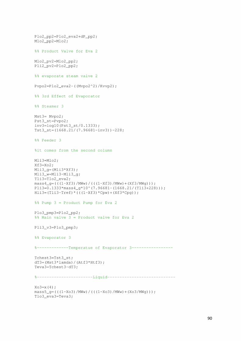
90
Plo2_pp2=Plo2_eva2+dP_pp2; Mlo2_pp2=Mlo2; %% Product Valve for Eva 2 Mlo2_pv2=Mlo2_pp2; Pli2_pv2=Plo2_pp2; %% evaporate steam valve 2 Pvpo2=Plo2_eva2-((Mvpo2^2)/Kvvp2); %% 3rd Effect of Evaporator %% Steamer 3 Mst3= Mvpo2; Pst3_st=Pvpo2; inv3=log10(Pst3_st/0.1333); Tst3_st=(1668.21/(7.96681-inv3))-228; %% Feeder 3 %it comes from the second column Mli3=Mlo2; Xf3=Xo2; Mli3_g=(Mli3*Xf3); Mli3_w=Mli3-Mli3_g; Tli3=Tlo2_eva2; mass4_g=(((1-Xf3)/MWw)/(((1-Xf3)/MWw)+(Xf3/MWg))); Pli3=0.1333*mass4_g*10^(7.96681-(1668.21/(Tli3+228))); Hli3=(Tli3-Tref)*(((1-Xf3)*Cpw)+(Xf3*Cpg)); %% Pump 3 = Product Pump for Eva 2 Plo3_pmp3=Plo2_pp2; %% Main valve 3 = Product valve for Eva 2 Pli3_v3=Plo3_pmp3; %% Evaporator 3 %-------------Temperatue of Evaporator 3----------------- Tchest3=Tst3_st; dT3=(Mst3*lamda)/(Atf3*Htf3); Teva3=Tchest3-dT3; %-----------------------Liquid---------------------------- Xo3=x(4); mass5_g=(((1-Xo3)/MWw)/(((1-Xo3)/MWw)+(Xo3/MWg))); Tlo3_eva3=Teva3;

91
Plo3_eva3=0.1333*mass5_g*10^(7.96681-(1668.21/(Tlo3_eva3+228))); %pressure of the product liquid, pressure of product liquid = pressure of feed liquid Plo3_v3=Plo3_eva3; %Pli_eva=Plo_eva Mlo3=(Xf3/Xo3)*Mli3;%mass of glycol feed = mass of glycol produce. Mlo3_g=(Xo3*Mlo3); Mlo3_w=((1-Xo3)*Mlo3); Hlo3=(Tlo3_eva3-Tref)*(((1-Xo3)*Cpw)+(Xo3*Cpg)); Klv3=((Mli3^2)/(Pli3_v3-Plo3_v3)); %Liquid valve coefficient in second column Kpv2=Klv3; Plo2_pv2=Plo3_eva3;%Pressure after the product valve in 2nd evaporator %--------------Steam produce from Evaporator 2------------ Mvpo3=Mli3-Mlo3; %mass balance Tvpo3_eva3=Teva3; Psto_eva3=0.1333*10^(7.96681-(1668.21/(Tvpo3_eva3+228))); Hsto_eva3=((Tvpo3_eva3-Tref)*Cpw)+lamda; %-------------Energy Balances------------- EB3=(Mli3*(Hli3-Hlo3))-(Mvpo3*(Hsto_eva3-Hlo3))+(Mst3*lamda); % to check whether the assuming of Xo2 is reliable or not %% Evaporate steam valve 3 Pvpo3=Plo3_eva3-((Mvpo3^2)/Kvvp3); %% Result Z=[EB EB2 EB3 Mst Xo Xo2 Xo3]; disp(' EB_Eva1 EB_Eva2 EB_Eva3 Mst Xo Xo2 Xo3'); disp(Z)
4. Single effect evaporator ‘FSolve’ simulation
a) main file
function F=eva_single_fsolve_vOptACM(x) Xo=x(1); Mst=x(2); Mli=x(3); Mlo=x(4); Mvpo=x(5); Teva=x(6); %constant % Psti=120.7815; dP=44.27; Klv=185; Tref=60; CpW=4.183; CpG=2.4; lamda=2080.8; Htf=150; Atf=168; Xi=0.035; Tli=88; Kvvp=521.33; MwW=18.02; MwG=62; %Temperature of the evaporator

92
% Psto=Psti-((Mst^2)/Ksv); % Tsto=(1668.21/(7.96681-log10(0.1333/Psto)))-228; %temperature of steam into evaporator dT=(lamda*Mst)/(Htf*Atf); Tchest=Teva+dT; %Mvpo %Entahlphy Hli=(Tli-Tref)*(((1-Xi)*CpW)+(Xi*CpG)); %feed liquid entahlphy Hlo=(Teva-Tref)*(((1-Xo)*CpW)+(Xo*CpG)); %product liquid entahlphy Hvo=((Teva-Tref)*CpW)+lamda; %entahlphy of vapour that produce by evaporator %Optimisation from ACM Exp1= -((Xi^0.2)*(Mlo*Xo)*700); Exp2= 0.7*Mst*(Tchest-50); xA=Mli-Mlo-Mvpo; %mass balance xB=(Xi*Mli)-(Xo*Mlo); %glycol balance xC=(Mli*(Hli-Hlo))-(Mvpo*(Hvo-Hlo))+(Mst*lamda); %energy balance xD=Teva-100; xE=Exp1+Exp2; F=[xA; xB; xC; xD; xE];
b) solver file
%single evaporator fsolve script % initial guest % Xo=x(1); % Mst=x(2); % Mli=x(3); % Mlo=x(4); % Mvpo=x(5); % Teva=x(6); clear Mlo0=37; Mst0=42; Mvpo0=40.0; Xo0=0.07; Mli0=77; Teva0=100; x0=[Xo0; Mst0; Mli0; Mlo0; Mvpo0; Teva0]; options=optimset('Algorithm','levenberg-marquardt','MaxFunEvals',1e12,'MaxIter',1000,'Display','iter'); [x,fval]=fsolve(@eva_single_fsolve_vOptACM,x0,options); %constant from ACM example % Ksv=46.361;Klv=185; Tref=60; CpW=4.183; CpG=2.4; lamda=2080.8; Htf=150; Atf=168; Xi=0.035; dP=44.27;

93
MwW=18.02; MwG=62; Kvvp=521.33; Xo=(x(1,1)); Mst=(x(2,1)); Mli_eva=(x(3,1)); Mlo_eva=(x(4,1)); Mvpo_eva=(x(5,1)); Teva=(x(6,1)); %Steam from boiler dT=(lamda*Mst)/(Htf*Atf) Tchest=dT+Teva; Tsti=105 Psti=0.1333*10^(7.96681-(1668.21/(Tsti+228))) Psto=0.1333*10^(7.96681-(1668.21/(Tchest+228))) Ksv=((Mst^2)/(Psti-Psto)) % Tsto=(1668.21/(7.96681-log10(Psto/0.1333)))-228 %temperature of steam into evaporator %liquid from feeder Tli=88 Pli=100 Mli=Mli_eva Mli_g=Xi*Mli Mli_w=(1-Xi)*Mli Hli=(Tli-Tref)*(((1-Xi)*CpW)+(Xi*CpG)) %liquid at the pump Plo_pmp=Pli+dP; %liquid at main valve Pli_v=Plo_pmp Plo_eva=0.1333*10^(7.96681-(1668.21/(Teva+228)))*(((1-Xo)/MwW)/(((1-Xo)/MwW)+(Xo/MwG))) %Plo_v is equal to Pli_eva where Pli_eva equal to Plo_eva Plo_v=Plo_eva Klv=((Mli^2)/(Pli_v-Plo_v)) %evaporator Tlo_eva=Teva Tvpo_eva=Teva dT_compare=Tchest-Teva; Mlo=Mlo_eva Mlo_g=Xo*Mlo Mlo_w=(1-Xo)*Mlo Pli_eva=Plo_v Hlo=(Teva-Tref)*(((1-Xo)*CpW)+(Xo*CpG)) Hvo=((Teva-Tref)*CpW)+lamda %vapour valve Pvpo=Pli_eva-((Mvpo_eva^2)/Kvvp)

94
5. Double effect evaporator ‘FSolve’ simulation
a) Main file
function F=eva_double_fsolve_optACM(x) Xo=x(1); Mst=x(2); Mli=x(3); Mlo=x(4); Mvpo=x(5); Teva=x(6); Mlo2=x(7); Mvpo2=x(8); Xo2=x(9); Teva2=x(10); %constant first effect % Psti=120.7815; % dP=44.27; Klv=185; % MwW=18.02; MwG=62; Tref=60; CpW=4.183; CpG=2.4; lamda=2080.8; Htf=150; Atf=168; Xi=0.035; Tli=88; Kvvp2=703.35; MwW=18.02; MwG=62; %constant second effect Htf2=80; Atf2=145; %Temperature of the evaporator % Psto=Psti-((Mst^2)/Ksv); % Tsto=(1668.21/(7.96681-log10(0.1333/Psto)))-228; %temperature of steam into evaporator % dT=(lamda*Mst)/(Htf*Atf); % Tchest=Teva+dT; massg=(((1-Xo2)/MwW)/(((1-Xo2)/MwW)+((Xo2)/MwG))); Pli_eva2=0.1333*10^(7.96681-(1668.21/(Teva2+228)))*massg; Pvpo_eva2=Pli_eva2-((Mvpo2^2)/Kvvp2); dT=(lamda*Mst)/(Htf*Atf); Tchest=Teva+dT; dT2=(lamda*Mvpo)/(Htf2*Atf2); Tchest2=Teva2+dT2; %Entahlphy first effect Hli=(Tli-Tref)*(((1-Xi)*CpW)+(Xi*CpG)); %feed liquid entahlphy Hlo=(Teva-Tref)*(((1-Xo)*CpW)+(Xo*CpG)); %product liquid entahlphy Hvo=((Teva-Tref)*CpW)+lamda; %entahlphy of vapour that produce by evaporator %Entahlphy second effect Hli2=(Teva-Tref)*(((1-Xo)*CpW)+(Xo*CpG)); Hlo2=(Teva2-Tref)*(((1-Xo2)*CpW)+(Xo2*CpG)); Hvo2=((Teva2-Tref)*CpW)+lamda;

95
%Optimisation from ACM Exp1= -((Xi^0.2)*(Mlo*Xo)*700); Exp2= (-80*Mst)-10*Mvpo2*(101.3-Pvpo_eva2); Exp3= (-95*Mlo2)+((Xo2^0.2)*(700*Mlo2)); Exp4= 0.7*Mst*(Tchest-50); Exp5= 0.7*Mvpo*(Tchest2-50); xA=Mli-Mlo-Mvpo; %mass balance first effect xB=(Xi*Mli)-(Xo*Mlo); %glycol balance first effect xC=(Mli*(Hli-Hlo))-(Mvpo*(Hvo-Hlo))+(Mst*lamda); %energy balance first balance xD=Mlo-Mlo2-Mvpo2; %mass balance second effect xE=(Xo*Mlo)-(Xo2*Mlo2); %glycol balance second effect xF=(Mlo*(Hli2-Hlo2))-(Mvpo2*(Hvo2-Hlo2))+(Mvpo*lamda); %energy balance second effect xG=Exp1+Exp2+Exp3+Exp4+Exp5; xH=Teva-100; xI=Xo2-0.12; F=[xA; xB; xC; xD; xE; xF; xG; xH; xI];
b) Solver file
%single evaporator fsolve script % initial guest % Xo=x(1); % Mst=x(2); % Mli=x(3); % Mlo=x(4); % Mvpo=x(5); % Teva=x(6); % Mlo2=x(7); % Mvpo2=x(8); % Xo2=x(9); % Teva2=x(10); clear % Ksv=46.361; Klv=185; Mlo0=27.7; Mvpo0=15; Mst0=16; Xo0=0.054; Mli0=42.8; Teva0=100; Mlo2i=12.5; Mvpo2i=15.2; Xo2i=0.12; Teva2i=96; x0=[Xo0; Mst0; Mli0; Mlo0; Mvpo0; Teva0; Mlo2i; Mvpo2i; Xo2i; Teva2i]; options=optimset('Algorithm','levenberg-marquardt','MaxFunEvals',1e12,'MaxIter',1000,'Display','iter'); [x,fval]=fsolve(@eva_double_fsolve_optACM,x0,options); %constant from ACM example Tref=60; CpW=4.183; CpG=2.4; lamda=2080.8; Htf=150; Atf=168; Htf2=80; Atf2=145; Xi=0.035; dP=44.27; dP2=10; dP_pro=90.3; MwW=18.02; MwG=62; Kvvp=521.33; Kvvp2=703.35; Plo_v_pro=120; %pressure product valve in 2nd effect Xo=(x(1,1)); Mst=(x(2,1));

96
Mli_eva=(x(3,1)); Mlo_eva=(x(4,1)); Mvpo_eva=(x(5,1)); Teva=(x(6,1)); Mlo2_eva=(x(7,1)); Mvpo2_eva=(x(8,1)); Xo2=(x(9,1)); Teva2=(x(10,1)); %% First Effect %Steam from boiler Tsti=105 Psti=0.1333*10^(7.96681-(1668.21/(Tsti+228))) dT=(lamda*Mst)/(Htf*Atf) Tchest=Teva+dT Psto=0.1333*10^(7.96681-(1668.21/(Tchest+228))) % Tsto=(1668.21/(7.96681-log10(Psto/0.1333)))-228 %temperature of steam into evaporator Ksv=((Mst^2)/(Psti-Psto)) %liquid from feeder Tli=88 Pli=100 Mli=Mli_eva Mli_g=Xi*Mli Mli_w=(1-Xi)*Mli Hli=(Tli-Tref)*(((1-Xi)*CpW)+(Xi*CpG)) %liquid at the pump Plo_pmp=Pli+dP; %liquid at main valve Pli_v=Plo_pmp Plo_v=0.1333*10^(7.96681-(1668.21/(Teva+228)))*(((1-Xo)/MwW)/(((1-Xo)/MwW)+(Xo/MwG))) %Plo_v is equal to Pli_eva and Pli_eva will equal to Plo_eva by the assumption from the study case Klv=((Mli^2)/(Pli_v-Plo_v)) %evaporator Tlo_eva=Teva Tvpo_eva=Teva dT_compare=Tchest-Teva; Mlo=Mlo_eva Mlo_g=Xo*Mlo Mlo_w=(1-Xo)*Mlo Pli_eva=Plo_v Plo_eva=Plo_v Hlo=(Teva-Tref)*(((1-Xo)*CpW)+(Xo*CpG)) Hvo=((Teva-Tref)*CpW)+lamda %vapour valve Pvpi=0.1333*10^(7.96681-(1668.21/(Teva+228))) Pvpo=Pli_eva-((Mvpo_eva^2)/Kvvp) %% Second Effect

97
%Steam from first effect dT2=(lamda*Mvpo_eva)/(Htf2*Atf2) Tsto2=(1668.21/(7.96681-log10(Pvpo/0.1333)))-228 Tchest2=Teva2+dT2 %Liquid from first effect Mli2=Mlo_eva Xi2=Xo Mli2_g=Xi2*Mli2 Mli2_w=(1-Xi2)*Mli2 Pli2=Plo_eva Tli2=Tlo_eva %liquid at the feed pump2 Plo_pmp2=Pli2+dP2 %liquid at the main valve2 Plo2_v=0.1333*10^(7.96681-(1668.21/(Teva2+228)))*(((1-Xo2)/MwW)/(((1-Xo2)/MwW)+(Xo2/MwG))) Pli2_v=Plo_pmp2 Klv2=((Mli2^2)/(Pli2_v-Plo2_v)) %evaporator2 dT2_compare=Tchest2-Teva2 Mlo2=Mlo2_eva Mlo2_g=Xo2*Mlo2 Mlo2_w=(1-Xo2)*Mlo2 Plo_eva2=Plo2_v Pli_eva2=Plo_eva2 Hlo2=(Teva2-Tref)*(((1-Xo2)*CpW)+(Xo2*CpG)) Hvo2=((Teva2-Tref)*CpW)+lamda %product pump in second effect Plo_pmp_pro=Plo_eva2+dP_pro %product valve in second effect Pli_v_pro=Plo_pmp_pro Kpv=(Mlo2^2)/(Pli_v_pro-Plo_v_pro) %vapour valve 2 Pvpi2=0.1333*10^(7.96681-(1668.21/(Teva2+228))) Pvpo2=Pli_eva2-((Mvpo2_eva^2)/Kvvp2)

98
6. Triple effect evaporator ‘FSolve’ simulation
a) Main file
function F=eva_triple_fsolve_vOptACM(x) Xo=x(1); Mst=x(2); Mli=x(3); Mlo=x(4); Mvpo=x(5); Teva=x(6); Mlo2=x(7); Mvpo2=x(8); Xo2=x(9); Teva2=x(10); Mlo3=x(11); Mvpo3=x(12); Xo3=x(13); Teva3=x(14); %we need to put mvpo as fixed value because if it is run by fsolve the %final product concentration will exceed 1 which not make any sense. %constant first effect % Psti=120.7815; % dP=44.27; Klv=185; % MwW=18.02; MwG=62; Tref=60; CpW=4.183; CpG=2.4; lamda=2080.8; Htf=150; Atf=168; Xi=0.035; Tli=88; MwW=18.02;MwG=62.0; Kvvp2=503.35; %constant second effect Htf2=80; Atf2=145; Htf3=65; Atf3=130; %Temperature of the evaporator % Psto=Psti-((Mst^2)/Ksv); % Tsto=(1668.21/(7.96681-log10(0.1333/Psto)))-228; %temperature of steam into evaporator massg=(((1-Xo2)/MwW)/(((1-Xo2)/MwW)+((Xo2)/MwG))); Pli_eva2=0.1333*10^(7.96681-(1668.21/(Teva2+228)))*massg; Pvpo_eva2=Pli_eva2-((Mvpo2^2)/Kvvp2); dT=(lamda*Mst)/(Htf*Atf); Tchest=Teva+dT; dT2=(lamda*Mvpo)/(Htf2*Atf2); Tchest2=Teva2+dT2; dT3=(lamda*Mvpo2)/(Htf3*Atf3); Tchest3=Teva3+dT3; % dT=(lamda*Mst)/(Htf*Atf);

99
% Tchest=Teva+dT; %Entahlphy first effect Hli=(Tli-Tref)*(((1-Xi)*CpW)+(Xi*CpG)); %feed liquid entahlphy Hlo=(Teva-Tref)*(((1-Xo)*CpW)+(Xo*CpG)); %product liquid entahlphy Hvo=((Teva-Tref)*CpW)+lamda; %entahlphy of vapour that produce by evaporator %Entahlphy second effect Hli2=(Teva-Tref)*(((1-Xo)*CpW)+(Xo*CpG)); Hlo2=(Teva2-Tref)*(((1-Xo2)*CpW)+(Xo2*CpG)); Hvo2=((Teva2-Tref)*CpW)+lamda; %Enthalphy third effect Hli3=(Teva2-Tref)*(((1-Xo2)*CpW)+(Xo2*CpG)); Hlo3=(Teva3-Tref)*(((1-Xo3)*CpW)+(Xo3*CpG)); Hvo3=((Teva3-Tref)*CpW)+lamda; %Optimisation from ACM Exp1= -((Xi^0.2)*(Mlo*Xo)*700); Exp2= (-80*Mst)-10*Mvpo2*(101.3-Pvpo_eva2); Exp3= (-95*Mlo2)+((Xo2^0.2)*(700*Mlo2)); Exp4= (-95*Mlo3)+((Xo3^0.2)*(700*Mlo3)); Exp5= 0.7*Mst*(Tchest-50); Exp6= 0.7*Mvpo*(Tchest2-50); Exp7= 0.7*Mvpo2*(Tchest3-50); xA=Mli-Mlo-Mvpo; %mass balance first effect xB=(Xi*Mli)-(Xo*Mlo); %glycol balance first effect xC=(Mli*(Hli-Hlo))-(Mvpo*(Hvo-Hlo))+(Mst*lamda); %energy balance first balance xD=Mlo-Mlo2-Mvpo2; %mass balance second effect xE=(Xo*Mlo)-(Xo2*Mlo2); %glycol balance second effect xF=(Mlo*(Hli2-Hlo2))-(Mvpo2*(Hvo2-Hlo2))+(Mvpo*lamda); %energy balance second effect xG=Mlo2-Mlo3-Mvpo3; %mass balance third effect xH=(Xo2*Mlo2)-(Xo3*Mlo3); %glycol balance second effect xI=(Mlo2*(Hli3-Hlo3))-(Mvpo3*(Hvo3-Hlo3))+(Mvpo2*lamda);%energy balance second effect xJ=Xo2-0.09261;%Constraint xK=Exp1+Exp2+Exp3+Exp4+Exp5+Exp6+Exp7;% xL=Teva-100; F=[xA; xB; xC; xD; xE; xF; xG; xH; xI; xJ; xK; xL];
b) Solver file
%single evaporator fsolve script % initial guest % Xo=x(1); % Mst=x(2); % Mli=x(3); % Mlo=x(4); % Mvpo=x(5);

100
% Teva=x(6); % Mlo2=x(7); % Mvpo2=x(8); % Xo2=x(9); % Teva2=x(10); % Mlo3=x(11); % Mvpo3=x(12); % Xo3=x(13); % Teva3=x(14); clear Mlo0=68.3; Mst0=32.5; Xo0=0.05; Mli0=98.5; Mvpo0=30.2; Teva0=100; Mlo2i=37.2; Mvpo2i=31.1; Xo2i=0.092; Teva2i=93; Mlo3i=5.5; Mvpo3i=31.7; Xo3i=0.6; Teva3i=84.7; x0=[Xo0; Mst0; Mli0; Mlo0; Mvpo0; Teva0; Mlo2i; Mvpo2i; Xo2i; Teva2i; Mlo3i; Mvpo3i; Xo3i; Teva3i]; options=optimset('Algorithm','levenberg-marquardt','MaxFunEvals',1e12,'MaxIter',3000,'Display','iter'); [x,fval]=fsolve(@eva_triple_fsolve_vOptACM,x0,options); %constant from ACM example % Ksv=46.361; Klv=185; Tref=60; CpW=4.183; CpG=2.4; lamda=2080.8; Htf=150; Atf=168; Htf2=80; Atf2=145; Htf3=65; Atf3=130; dP=44.27; dP2=10; dP3=90.3; Xi=0.035;MwW=18.02; MwG=62; Kvvp=521.33; Kvvp2=703.35; Kvvp3=703.35; %pressure product valve in 2nd effect Xo=(x(1,1)); Mst=(x(2,1)); Mli_eva=(x(3,1)); Mlo_eva=(x(4,1)); Mvpo_eva=(x(5,1)); Teva=(x(6,1)); Mlo2_eva=(x(7,1)); Mvpo2_eva=(x(8,1)); Xo2=(x(9,1)); Teva2=(x(10,1)); Mlo3_eva=(x(11,1)); Mvpo3_eva=(x(12,1)); Xo3=(x(13,1)); Teva3=(x(14,1)); %% First Effect %Steam from boiler Tsti=105 Psti=0.1333*10^(7.96681-(1668.21/(Tsti+228))) dT=(lamda*Mst)/(Htf*Atf) Tchest=dT+Teva Psto=0.1333*10^(7.96681-(1668.21/(Tchest+228))) Tsto=(1668.21/(7.96681-log10(Psto/0.1333)))-228 %temperature of steam into evaporator Ksv=((Mst^2)/(Psti-Psto)) %liquid from feeder Tli=88

101
Pli=100 Mli=Mli_eva Mli_g=Xi*Mli Mli_w=(1-Xi)*Mli Hli=(Tli-Tref)*(((1-Xi)*CpW)+(Xi*CpG)) %liquid at the pump Plo_pmp=Pli+dP; %liquid at main valve Pli_v=Plo_pmp Plo_eva=0.1333*10^(7.96681-(1668.21/(Teva+228)))*(((1-Xo)/MwW)/(((1-Xo)/MwW)+(Xo/MwG))) Plo_v=Plo_eva %Pli is equal to Plo of evaporator, and plo_v=Pli_eva Klv=((Mli^2)/(Pli_v-Plo_v)) %evaporator Tlo_eva=Teva Tvpo_eva=Teva Mlo=Mlo_eva Mlo_g=Xo*Mlo Mlo_w=(1-Xo)*Mlo Pli_eva=Plo_v Hlo=(Teva-Tref)*(((1-Xo)*CpW)+(Xo*CpG)) Hvo=((Teva-Tref)*CpW)+lamda %vapour valve Pvpi=0.1333*10^(7.96681-(1668.21/(Teva+228))) Pvpo=Pli_eva-((Mvpo_eva^2)/Kvvp) %% Second Effect %Steam from first effect Tsto2=(1668.21/(7.96681-log10(Pvpo/0.1333)))-228 dT2=(lamda*Mvpo_eva)/(Htf2*Atf2) Tchest2=Teva2+dT2 %Liquid from first effect Mli2=Mlo_eva Xi2=Xo Mli2_g=Xi2*Mli2 Mli2_w=(1-Xi2)*Mli2 Pli2=Plo_eva Tli2=Tlo_eva %liquid at the feed pump2 Plo_pmp2=Pli2+dP2 %liquid at the main valve2 Plo2_v=0.1333*10^(7.96681-(1668.21/(Teva2+228)))*(((1-Xo2)/MwW)/(((1-Xo2)/MwW)+(Xo2/MwG))) Pli2_v=Plo_pmp2 Klv2=((Mli2^2)/(Pli2_v-Plo2_v)) %evaporator2 Tlo_eva2=Teva2

102
Tvpo_eva2=Teva2 dT2_compare=Tchest2-Teva2 Mlo2=Mlo2_eva Mlo2_g=Xo2*Mlo2 Mlo2_w=(1-Xo2)*Mlo2 Plo_eva2=Plo2_v Pli_eva2=Plo_eva2 Hlo2=(Teva2-Tref)*(((1-Xo2)*CpW)+(Xo2*CpG)) Hvo2=((Teva2-Tref)*CpW)+lamda %vapour valve 2 % Pvpo2=0.1333*10^(7.96681-(1668.21/(Teva2+228))) % Kvvp2=((Mvpo2_eva^2)/(Pli_eva2-Pvpo2)) Pvpo2=Pli_eva2-((Mvpo2_eva^2)/Kvvp2) %% Triple Effect %Steam from first effect Tsto3=(1668.21/(7.96681-log10(Pvpo2/0.1333)))-228 dT3=(lamda*Mvpo2_eva)/(Htf3*Atf3) Tchest3=Teva3+dT3 %Liquid from second effect Mli3=Mlo2_eva Xi3=Xo2 Mli3_g=Xi3*Mli3 Mli3_w=(1-Xi3)*Mli3 Pli3=Plo_eva2 Tli3=Tlo_eva2 %liquid at the feed pump2 Plo_pmp3=Pli3+dP3 %liquid at the main valve2 Plo3_v=0.1333*10^(7.96681-(1668.21/(Teva3+228)))*(((1-Xo3)/MwW)/(((1-Xo3)/MwW)+(Xo3/MwG))) Pli3_v=Plo_pmp3 Klv3=((Mli3^2)/(Pli3_v-Plo3_v)) %evaporator2 dT3_compare=Tchest3-Teva3 Mlo3=Mlo3_eva Mlo3_g=Xo3*Mlo3 Mlo3_w=(1-Xo3)*Mlo3 Plo_eva3=Plo3_v Pli_eva3=Plo_eva3 Hlo3=(Teva3-Tref)*(((1-Xo3)*CpW)+(Xo3*CpG)) Hvo3=((Teva3-Tref)*CpW)+lamda %vapour valve 3 Pvpo3=Pli_eva3-((Mvpo3_eva^2)/Kvvp3) % Kvvp3=((Mvpo3_eva^2)/(Pli_eva3-Pvpo3))