Scattering of Electromagnetic Radiation by

Complex Microstructures in the Resonant Regime

Erik Shepard Thiele

A DISSERTATION •

Ill

Materials Science and Engineering

Presented to the Faculties of the University of Pennsylvania in Partial Fulfillment of the

Requirements for the Degree of Doctor of Philosophy.

1998

Supervisor of Dissertation

ii

Copyright

By

Erik Shepard Thiele

1998

iii

Dedication

To my family.

iv

Acknowledgments

I begin by thanking and applauding my research advisor, Roger French, who

first encouraged me to embark on this journey. Roger has helped me to appreciate the

real point of forming a piece of work like this thesis. His support and guidance has

been indispensable, and without these I would have missed out on most of the deep

satisfaction of this process. I am very grateful to my faculty advisor, Peter Davies,

whom I have had the good fortune of knowing since my undergraduate days. I have

always respected Peter for his scientific leadership, but even more for his genuine

concern for all of us who have worked with him. I am also very thankful for the

guidance and encouragement I have received from Professors Dawn Bonnell and

Takeshi Egami throughout the development of this dissertation.

By far the most satisfying aspect of this experience has been the enjoyment of

working (and playing) with so many terrific people along the way. Naming all of you

here might actually prevent my being able to finish what writing I have yet to complete,

so I don’t dare try! You know who you are. I also wish to express my gratitude to the

DuPont Company and to my management, past and present, for supporting this

research. I recognize what a unique opportunity they have provided me.

Finally, I want to give thanks for that handful of very special people of whom life has

seemingly made gifts to me. My family means the world to me, and I appreciate this

today more than ever. Dear friends like Mike, Mark, Claire, Eric, Mike, Tom, Phil, and

Claudio are treasures. Though our paths cross and diverge over time, these people are

v

like stars in the sky, always with me. Alors, je finis en remerciant avec un coeur bien

joyeux ma femme du désert, le vrai trésor au bout de cette chapitre-ci de ma légende

personnelle. Tu me fait m’épanouir, bellissima, et je t’aime! Vraiment, je serai avec toi

pour toujours.

vi

Abstract

A computational optics approach is used to determine the scattering properties

of complex microstructures in the resonant regime. The time-domain finite element

method employed in this research to solve Maxwell’s equations can be used to

determine the scattering properties of scattering systems exhibiting arbitrary, complex

shapes and optical anisotropy. A detailed study of the factors influencing the accuracy

of this numerical method demonstrates that the construction of the finite element model

strongly influences accuracy; error in these computations is confined to <3% for typical

models. The computational optics approach is applied to determine the light scattering

efficiencies of several different white pigment systems. It is demonstrated that the light

scattering efficiency of core-shell white pigment particles is limited by the content of

low-index material and therefore cannot attain the same efficiency as optimized

particles of the high-index material. Optically anisotropic spheres of rutile titania

exhibit the expected dependence of scattering properties upon the angle of light

incidence and polarization. Under conditions of random illumination, the scattering

efficiencies of these spheres can be approximated to within 10% using models based

upon isotropic materials. The agglomeration of both colloidal titania and latex particles

causes substantial deviation from the light scattering properties of the isolated primary

particles. In the case of rutile titania particles of optimal size, for example, losses in

volume-normalized scattering efficiency of 70% occur for the largest agglomerates

studied. The use of single, equivalent mass spheres to approximate the light scattering

properties of the agglomerate structures succeeds in predicting trends in these properties

vii

but fails as a rigorous description of these properties. For small clusters of either latex

or titania particles with varying interparticle separation distance, optical interactions

between neighboring particles diminish rapidly with increasing particle separation. In

most cases, changes in scattering efficiency with interparticle separation distance could

be well fit using an exponential decay. The decay constant of these spatial variations

varies in the range 0.25-0.45 light wavelengths for these systems, with appreciable

optical interactions not extending beyond 2-3 light wavelengths.

viii

Table of Contents

Scattering of Electromagnetic Radiation by ........................................................................ i Complex Microstructures in the Resonant Regime ............................................................. i Dedication.......................................................................................................................... iii Acknowledgments ............................................................................................................. iv Abstract.............................................................................................................................. vi Table of Contents............................................................................................................. viii List of Tables ..................................................................................................................... xi List of Illustrations............................................................................................................ xii Chapter 1. Introduction.......................................................................................................1

1.1 Single Scattering.......................................................................................................1 1.2 Scattering by Ensembles of Scattering Features.......................................................4 1.3 Formulation of the Present Research........................................................................6 1.4 On Vector Notation ..................................................................................................7

Chapter 2. Literature Review..............................................................................................8 2.1 Electromagnetic Radiation Scattering in Materials Science.....................................8 2.2 Light Scattering Properties of Complex Microstructures.........................................9

2.2.1 Light Scattering by White Pigment Particles.....................................................9 2.2.1.1 Application of Mie Theory to Optically Anisotropic Materials ...............11 2.2.1.2 Kubelka-Munk Analysis of Paint Film Scattering Efficiencies ...............12 2.2.1.3 Computational Modeling of Scattering by White Pigments: Previous Studies....................................................................................................................14

2.2.2 Light Scattering by Concentrated Particle Dispersions ...................................16 2.2.2.1 The Crowding Effect in Paint Films.........................................................16 2.2.2.2 Light Scattering in Stereolithography.......................................................21

2.2.3 Light Scattering by Particle Agglomerates......................................................23 2.2.3.1 Computational Approaches ......................................................................23 2.2.3.2 Computational Results for Particle Agglomerates ...................................25

2.3 Principles of Light Scattering ..................................................................................27 2.3.1 Maxwell’s Equations .......................................................................................27 2.3.2 Exact, Analytical Solutions of Light Scattering ..............................................30 2.3.3 Approximate and Numerical Solutions of Light Scattering ............................33

2.3.3.1 Rayleigh Theory .......................................................................................33 2.3.3.2 Geometrical Optics ...................................................................................35 2.3.3.3 Point Matching..........................................................................................38 2.3.3.4 Perturbation Methods................................................................................38 2.3.3.5 Coupled-Dipole Method ...........................................................................39 2.3.3.6 T-Matrix or Extended Boundary Condition Method ................................41 2.3.3.7 Method of Moments .................................................................................42 2.3.3.8 Finite Difference Time-Domain Method..................................................45 2.2.3.9 Finite Element Method .............................................................................47

Chapter 3. Computational Methods..................................................................................55

ix

3.1 Mie Theory .............................................................................................................55 3.1.1 Computation of the Scattering Coefficients an and bn .....................................55 3.1.2 Far-Field Scattering Parameters.......................................................................59

3.2 Finite Element Time-Domain Method ...................................................................62 3.2.1 Numerical Implementation ..............................................................................63 3.2.2 Use of the EMFlex Software in Practice .........................................................67 3.2.3 Computation of Far-Field Scattering Parameters ............................................68 3.2.4 Simulation of Random Illumination: The Illuminator.....................................69

Chapter 4. Performance of the Time-Domain Finite Element Method ............................75 4.1 Materials System of Interest ...................................................................................75 4.2 Computational Efficiency.......................................................................................82

4.2.1 Memory Requirements For Finite Element Computations..............................82 4.2.2 CPU Time Requirements For Finite Element Computations ..........................83 4.2.3 CPU Time Requirements For Far-Field Extrapolation....................................84

4.3 Computational Accuracy ........................................................................................87 4.3.1 Effects of Finite Element Mesh Density..........................................................87 4.3.2 Effects of Mesh Density on Surface of Far Field Sphere ................................90 4.3.3 Effects of Far-Field Sphere Radius..................................................................91 4.3.4 Effects of Kirchoff Box Placement in the Model ............................................92 4.3.5 Effects of Particle Position Relative to Model Walls ......................................94 4.3.6 Effects of Model Dimensions Compared to Light Wavelength ......................97 4.3.7 Effects of Strong Resonance: High-Index Spheres in Vacuum.....................102

4.4 Guidelines For Building Robust Finite Element Models .....................................105 Chapter 5. A Potpourri of Pigment Particles ..................................................................106

5.1 Core-Shell Pigment Particles................................................................................107 5.1.1 Introduction....................................................................................................107 5.1.2 Scattering Properties of Titania-Coated Core-Shell Pigments ......................108

5.1.2.1 Refractive index of medium at 1.45 .......................................................110 5.1.2.2 Refractive index of medium at 1.0 (air)..................................................118

5.2 Anisotropic Spheres of Rutile Titania ..................................................................120 5.2.1 Introduction....................................................................................................120 5.2.2 Scattering By Anisotropic Spheres of Rutile Titania ....................................125 5.2.3 Angle and Polarization Dependence of Scattering by an Anisotropic Titania Sphere ......................................................................................................................131 5.2.4 On the Validity of the Average Index and Weighted Sum Approximations .132

5.3 Scattering by a Morphological Rutile Titania ......................................................136 5.3.1 Introduction....................................................................................................136 5.3.2 Scattering by a Morphological Rutile Particle...............................................138 5.3.3 Discussion......................................................................................................141

5.3.3.1 Scattering Coefficients of the Morphological Rutile Particle.................141 5.3.3.2 Mie Theory in Particle Size Analysis by Light Scattering .....................142

Chapter 6. Clusters of Latex Spheres: A Low-Contrast System ....................................145 6.1 Materials System of Interest .................................................................................146 6.2 Light Scattering by Latex Sphere Clusters of Increasing Size .............................150

x

6.3 Near-Field Interactions Between Neighboring Latex Particles ............................157 Chapter 7. Clusters of Titania Particles: A High-Contrast System ................................165

7.1 Materials Systems of Interest ................................................................................165 7.2 Light Scattering by Titania Sphere Clusters of Increasing Size ...........................168 7.3 Near-Field Interactions Between Neighboring Titania Particles..........................173 7.4 Near-Field Interactions Between Two Morphological Rutile Particles ...............176

Chapter 8. Discussion: Light Scattering by Complex Microstructures in the Resonant Regime.............................................................................................................................184

8.1 Accuracy of the Time-Domain Finite Element Method.......................................184 8.2 Light Scattering by Complex, Resonant Particles ................................................185 8.3 Light Scattering by Densely Packed Particle Aggregates ....................................188 8.4 Near-Field Optical Interactions Between Particles ..............................................195

8.4.1 Titania and Latex Systems.............................................................................195 8.4.2 Extension to Other Materials Systems...........................................................201

Chapter 9. Conclusions...................................................................................................203 Appendix. Typical EMFlex Input Deck .........................................................................207 Bibliography ....................................................................................................................210

xi

List of Tables

Table 1. Error in scattering cross section as a function of separation distance between the bottom of the sphere and the bottom wall of the model. The corresponding models are shown in Figure 20. .............................................................................. 97

Table 2. Error in scattering cross section of finite element calculations in which the model edge length was systematically varied. All calculations are for the case of a 40-nm sphere at the center of a cubic model. ....................................................... 101

Table 3. Error in scattering cross section of finite element calculations in which the model edge length was systematically varied. All calculations are for the case of a 200-nm sphere at the center of a cubic model. ..................................................... 101

Table 4. Error in scattering cross section as a function of sphere diameter for the three cases indicated on the plot in Figure 22................................................................ 104

Table 5. Scattering coefficients S and σ computed for anisotropic spheres of different diameter using the finite element approach. ......................................................... 130

Table 6. Values of χ2 (Equation 80) associated with S and σ values for the average index and weighted sum approximation, compared to anisotropic sphere scattering data generated using the finite element approach................................................. 135

Table 7. Comparison between the far-field scattering coefficients for the single rutile particle and the equivalent volume sphere, using both the average index and weighted sum approximations. ............................................................................. 143

Table 8. Diameters of spheres exhibiting the same far-field scattering coefficients as the single rutile particle, using both the average index and weighted sum approximations...................................................................................................... 143

Table 9. Diameters of spheres exhibiting the same far-field scattering coefficients as the system of two rutile particles for each interparticle separation distance considered, using both the average index and weighted sum approximations. ....................... 183

Table 10. Results of parametric fits of the six curves shown in Figure 69 and Figure 70 using the expression in Equation 81. .................................................................... 200

xii

List of Illustrations

Figure 1. Schematic diagram of scattering object size versus radiation wavelength identifying three scattering domains: geometrical optics, the resonant regime, and the Rayleigh scattering regime. ................................................................................ 4

Figure 2. The ordinary (lower, dashed curve) and extraordinary (upper, dotted curve) refractive indices of rutile titania versus light wavelength. These data were compiled from multiple sources by Ribarsky.13 ..................................................... 11

Figure 3. The scattering coefficient S* for rutile titania particles in a typical paint film as a function of pigment volume concentration. (After Braun25) .......................... 21

Figure 4. Schematic diagram of a stereolithography apparatus for producing complex ceramic parts using rapid prototyping. (After Liao.) ............................................. 23

Figure 5. Schematic diagram showing reflection and refraction of a light ray using the geometrical optics approximation. (After Bohren and Huffman1) ........................ 38

Figure 6. Flow chart showing the formulation and evaluation of light scattering problems using the Illuminator software. ............................................................... 73

Figure 7. A representation of the spherical illumination coordinate system used in Illuminator runs. In this case, there is an 18o increment in the spherical coordinate angles phi and theta between adjacent surface area elements. The individual illumination directions pass through the centers of the surface area elements....... 74

Figure 8. Dependence of the scattering coefficient S upon sphere diameter for the case of a sphere with n = 2.74 embedded in a resin with n = 1.51. The illumination wavelength is 560 nm. ............................................................................................ 78

Figure 9. Dependence of the angle-weighted scattering coefficient σ upon sphere diameter for the case of a sphere with n = 2.74 embedded in a resin with n = 1.51. The illumination wavelength is 560 nm. ................................................................ 78

Figure 10. Finite element model of a 200-nm sphere with n = 2.74 embedded in a polymeric resin with n = 1.51. The 560-nm illuminating light propagates in the +x direction and is polarized in the z direction. This model contains 1,340,000 volume elements. .................................................................................................... 79

Figure 11. Time history of z-polarized electric field amplitude at the center of the sphere shown in the computation of Figure 10....................................................... 80

Figure 12. Finite element model of a 200-nm sphere with n = 2.74 embedded in a polymeric resin with n = 1.51. The 560-nm illuminating light propagates in the +x direction and is polarized in the z direction. This model contains 168,000 volume elements. ................................................................................................................. 81

Figure 13. Dependence of Cray C-94 memory requirement upon the number of volume elements in the finite element model for the present series of EMFlex computations........................................................................................................... 83

Figure 14. Dependence of Cray C-94 CPU time requirement upon the number of volume elements in the finite element model for the present series of EMFlex computations........................................................................................................... 84

xiii

Figure 15. CPU time required for a single far-field extrapolation is shown in as a function of the angular discretization on the surface of the far-field sphere. ......... 86

Figure 16. CPU time required for a single far-field extrapolation is shown in as a function of the number of surface elements on the far-field sphere. ...................... 86

Figure 17. Error in scattering cross section compared to the exact result from Mie theory as a function of ρ, the number of volume elements in a model per minimum wavelength of the 560-nm light propagating in the finite element models. ........... 89

Figure 18. Error in scattering cross section compared to the exact result from Mie theory as a function of as a function of angular discretization on the surface of the far-field sphere surface. .......................................................................................... 91

Figure 19. Error in scattering cross section compared to the exact result from Mie theory as a function of as a function of far-field sphere radius. ............................. 92

Figure 20. Cross-sectional slices through the centers of four finite element models in which the spacing between the 200-nm sphere and the bottom wall of the model has been systematically varied. Scattered light intensity is shown in each case. .. 96

Figure 21. Finite element model of a 40-nm sphere with n = 2.74 embedded in a polymeric resin with n = 1.51. The 560-nm illuminating light propagates in the +x direction and is polarized in the z direction.......................................................... 100

Figure 22. The scattering coefficient S (µm−1) as a function of sphere diameter for the case of a sphere with n = 3.0 in a medium with n = 1.0. This represents a more resonant system than can be achieved in practice, since no known, non-lossy material exhibits such a high refractive index in the visible spectrum................. 104

Figure 23. Schematic representation of titania coated on a core particle of lower refractive index. .................................................................................................... 109

Figure 24. Scattering coefficient σ (µm−1) versus coated particle diameter and refractive index of the core material for titania-coated particles with coating thickness equal to 10% of the particle radius. ...................................................... 112

Figure 25. Scattering coefficient σ (µm−1) versus silica core diameter and titania shell diameter for a coated particle. The global maximum of this plot corresponds to a solid titania sphere of 0.2 µm diameter. ............................................................... 112

Figure 26. Scattering coefficient σ for five coated particles with different outside diameters............................................................................................................... 114

Figure 27. Scattering coefficient σ versus particle diameter for a solid titania sphere and a titania-coated silica particle with coating thickness equal to 10% of the particle radius........................................................................................................ 115

Figure 28. Scattering coefficient σ divided by the density of the coated particle. The global maximum of this plot corresponds to a solid titania sphere with no silica present................................................................................................................... 117

Figure 29. Scattering coefficient σ divided by the weight fraction of titania present in each coated particle. The global maximum of this plot corresponds to a solid titania sphere with no silica present...................................................................... 117

xiv

Figure 30. Scattering coefficient σ for the five particles shown in Figure 26, with the cellulose surrounding medium replaced by air (refractive index 1.0 instead of 1.45). ..................................................................................................................... 120

Figure 31. Scattering coefficient S versus sphere diameter for an optically isotropic sphere from Mie theory, using the average index approximation. ....................... 123

Figure 32. Angle-weighted scattering coefficient σ versus sphere diameter for an optically isotropic sphere from Mie theory, using the average index approximation............................................................................................................................... 123

Figure 33. Scattering coefficient S versus sphere diameter for an optically isotropic sphere from Mie theory, using the weighted sum approximation. ....................... 124

Figure 34. Angle-weighted scattering coefficient σ versus sphere diameter for an optically isotropic sphere from Mie theory, using the weighted sum approximation............................................................................................................................... 124

Figure 35. Finite element model and scattered intensities for a 0.2-µm anisotropic sphere of rutile titania. The 560-nm radiation propagates in the +x direction, with unit incident intensity. Polarization is parallel to the y direction. ....................... 128

Figure 36. The scattering coefficient S as a function of sphere diameter computed using the finite element method (solid points) for anisotropic spheres of rutile titania with n =2.74 embedded in a medium with n = 1.51. The illumination wavelength is 560 nm. The long dashed curve corresponds to the average index approximation, while the dotted curve corresponds to the weighted sum approximation....................... 129

Figure 37. The angle-weighted scattering coefficient σ as a function of sphere diameter computed using the finite element method (solid points) for anisotropic spheres of rutile titania embedded in a medium with n = 1.51. The illumination wavelength is 560 nm. The long dashed curve corresponds to the average index approximation, while the dotted curve corresponds to the weighted sum approximation............. 129

Figure 38. Scattering coefficient S as a function of the angle of incidence (relative to the optic axis) for the 0.2-µm anisotropic sphere of rutile titania. Hollow circles are for polarization perpendicular to the optic axis of the sphere; filled circles are for polarization coplanar with the optic axis. ....................................................... 132

Figure 39. High resolution scanning electron micrograph of rutile titania particles, showing their characteristic, morphological shapes. (Micrograph courtesy E.D. Boyes, DuPont Central Research and Development.) .......................................... 137

Figure 40. Finite element model and near field scattering results for an anisotropic, morphological rutile particle with a width of 0.175 µm, and a length of 0.35 µm in n = 1.51 resin; the light wavelength is 560 nm..................................................... 140

Figure 41. The scattering coefficient S as a function of sphere diameter for a latex particle with n = 1.50 in a water medium with n = 1.33. The illuminating light wavelength is 488 nm. The 200-nm sphere diameter studied in this chapter is marked with an “x.” .............................................................................................. 148

Figure 42. The angle-weighted scattering coefficient σ as a function of sphere diameter for a latex particle with n = 1.50 in a water medium with n = 1.33. The illuminating light wavelength is 488 nm. The 200-nm sphere diameter studied in this chapter is marked with an “x.”....................................................................... 148

xv

Figure 43. Finite element model for a 200-nm latex sphere with n = 1.50 in a water medium with n = 1.33. The illuminating wavelength is 488 nm, and light propagates in the +x direction............................................................................... 149

Figure 44. Finite element models of latex sphere clusters containing 3, 7, 13, and 27 spheres. ................................................................................................................. 154

Figure 45. Finite element model of a cluster of seven 200-nm latex spheres n = 1.50 in a water matrix with n = 1.33. The 488-nm illuminating light propagates in the +x direction and is polarized in the z direction.......................................................... 155

Figure 46. The scattering coefficient S as a function of the number of 200-nm latex particles composing a particle cluster under conditions of random illumination. 156

Figure 47. The quantity (1−g) as a function of the number of 200-nm latex spheres composing a particle cluster under conditions of random illumination................ 156

Figure 48. The scattering coefficient σ as a function of the number of 200-nm latex spheres composing a particle cluster under conditions of random illumination... 157

Figure 49. Finite element model of a cluster of seven 200-nm latex spheres n = 1.50 in a water matrix with n = 1.33. The surface-to-surface interparticle spacing is 0.4 µm. The 488-nm illuminating light propagates in the +x direction and is polarized in the z direction. .................................................................................................. 162

Figure 50. Dependence of the scattering coefficient S upon surface-to-surface interparticle separation distance for the clusters of seven latex spheres. The dashed line corresponds to the value associated with a single 200-nm latex primary particle. ................................................................................................................. 163

Figure 51. Dependence of the quantity (1−g) upon surface-to-surface interparticle separation distance for the clusters of seven latex spheres. The dashed line corresponds to the value associated with a single 200-nm latex primary particle............................................................................................................................... 163

Figure 52. Dependence of the angle-weighted scattering coefficient σ upon surface-to-surface interparticle separation distance for the clusters of seven latex spheres. The dashed line corresponds to the value associated with a single 200-nm latex primary particle. ................................................................................................................. 164

Figure 53. The scattering coefficient S as a function of sphere diameter for a rutile particle with n = 2.74 in a polymer medium with n = 1.51 under the average index approximation. The illuminating light wavelength is 560 nm. The 200-nm sphere diameter studied in this chapter is marked with an “x.” ....................................... 167

Figure 54. The angle-weighted scattering coefficient σ as a function of sphere diameter for a rutile particle with n = 2.74 in a polymer medium with n = 1.51 under the average index approximation. The illuminating light wavelength is 560 nm. The 200-nm sphere diameter studied in this chapter is marked with an “x.” .............. 167

Figure 55. Finite element model of a cluster of seven 200-nm titania spheres with n = 2.74 in a polymer matrix with n = 1.51. The 560-nm illuminating light propagates in the +x direction and is polarized in the z direction........................................... 171

Figure 56. The scattering coefficient S as a function of the number of 200-nm titania spheres composing a particle cluster. These results are for the case of random illumination of each cluster, resulting in orientation-averaged results................. 172

xvi

Figure 57. The scattering coefficient σ as a function of the number of 200-nm titania spheres composing a particle cluster. These results are for the case of random illumination of each cluster, resulting in orientation-averaged results................. 172

Figure 58. Dependence of the scattering coefficient S upon surface-to-surface interparticle separation distance for the clusters of seven titania spheres. The dashed line corresponds to the value associated with a single 200-nm titania primary particle..................................................................................................... 175

Figure 59. Dependence of the angle-weighted scattering coefficient σ upon surface-to-surface interparticle separation distance for the clusters of seven titania spheres. The dashed line corresponds to the value associated with a single 200-nm titania primary particle..................................................................................................... 175

Figure 60. Finite element model cross section and near field scattering results for two anisotropic morphological rutile particles in n = 1.51 resin for light incident normal to the cross section shown and with a wavelength of 560 nm. The interparticle spacing is 0.5 µm. ................................................................................................. 179

Figure 61. Finite element model cross section and near field scattering results for two anisotropic morphological rutile particles in n = 1.51 resin for light incident normal to the cross section shown and with a wavelength of 560 nm. The interparticle spacing is 0.3 µm. ................................................................................................. 180

Figure 62. Finite element model cross section and near field scattering results for two anisotropic morphological rutile particles in n = 1.51 resin for light incident normal to the cross section shown and with a wavelength of 560 nm. The interparticle spacing is 0 µm. .................................................................................................... 181

Figure 63. Scattering coefficient S for two morphological rutile particles as a function of interparticle separation. The horizontal line shows the results for one of the morphological rutile particles. .............................................................................. 182

Figure 64. Angle-weighted scattering coefficient σ for two morphological rutile particles as a function of interparticle separation. The horizontal line shows the results for one of the morphological rutile particles. ............................................ 182

Figure 65. The scattering coefficient S as a function of the number of 200-nm latex particles composing a particle cluster (solid curve). For comparison, the results of Mie theory computations on single, equivalent-mass spheres are shown (dashed curve). ................................................................................................................... 193

Figure 66. The scattering coefficient σ as a function of the number of 200-nm latex particles composing a particle cluster (solid curve). For comparison, the results of Mie theory computations on single, equivalent-volume spheres are shown (dashed curve). ................................................................................................................... 193

Figure 67. The scattering coefficient S as a function of the number of 200-nm titania particles composing a particle cluster (solid curve). For comparison, the results of Mie theory computations on single, equivalent-mass spheres are shown (dashed curve). ................................................................................................................... 194

Figure 68. The scattering coefficient σ as a function of the number of 200-nm titania particles composing a particle cluster (solid curve). For comparison, the results of

xvii

Mie theory computations on single, equivalent-mass spheres are shown (dashed curve). ................................................................................................................... 194

Figure 69. Scattering coefficient S (%) for the three different multiple-particle systems as a function of the center-to-center interparticle spacing expressed in wavelengths. The value 100% corresponds to the S value for an isolated primary particle in each case........................................................................................................................ 200

Figure 70. Angle-weighted scattering coefficient σ (%) for the three multiple-particle systems as a function of the center-to-center interparticle spacing expressed in wavelengths. The value 100% corresponds to the σ value for an isolated primary particle in each case. ............................................................................................. 201

1

Chapter 1. Introduction

Scattering phenomena underlie the human perception of the natural world

through the sense of sight, and the scattering properties of physical systems are widely

exploited in both science and technology. Scattering of electromagnetic radiation by

microstructures encompasses a broad range of physical phenomena. Wavelengths in the

electromagnetic spectrum span an infinite range, and those exploited technologically

range from kilometer-long radio signals to sub-angstrom gamma rays. The nature of the

scattering interaction between electromagnetic radiation and materials is determined

primarily by the relationship between radiation wavelength and the physical dimensions

of scattering features in materials systems. With an appreciation of this premise, a

unified view of electromagnetic radiation scattering by microstructures is possible,

spanning the orders of magnitude in size which exist in both the electromagnetic

spectrum and the physical world.

1.1 Single Scattering

The fundamental case in the analysis of electromagnetic radiation scattering is

that of single scattering, in which the interaction between radiation and a single,

isolated scattering feature is considered. Results of single scattering can be extended to

ensembles which contain a sufficiently small number of particles with interparticle

separations large enough that each particle develops its individual scattering pattern

without influence from its neighbors. A qualitative criterion for the assumption of

single scattering is that each particle in an ensemble experiences the same incident

2

electric field, with negligible scattered field from other features in the ensemble. The

treatment of an ensemble of scatterers in the single scattering regime is straightforward:

the scattering properties of the ensemble is simply the sum of contributions from the

individual scatterers.1,2

The degree of mathematical complexity in the treatment of the radiation

scattering by an isolated scattering feature is strongly affected by the relationship

between radiation wavelength and the physical size of a scattering feature, as suggested

above. In general, simplifying approximations can be applied to the separate cases in

which the wavelength is at least an order of magnitude greater or less than the size of a

scattering feature. The former case includes the well-known Rayleigh scattering theory

which explains the basis of the blue color of the daytime sky on a clear day, for

example, while the latter case includes the application of geometrical optics techniques

to the prediction of visible image formation by macroscopic objects. For cases in which

the wavelength of electromagnetic radiation is on the order of the size of a scattering

feature, the mathematical description of scattering is potentially intractable using even

the most sophisticated analytical approaches. This is especially true for material

systems exhibiting high optical contrast between the scattering feature and its

surrounding medium, since very strong coupling and resonance can occur. Scattering

efficiencies in this resonant regime can be very high. An example of one such system is

the scattering of visible light by an optimized white pigment particle, where near-field

scattered intensities in the vicinity of the particle can be an order of magnitude greater

than that of the incident light and the scattering cross section of a particle can be many

3

times greater than its geometric cross section. These domains of Rayleigh scattering,

the resonant regime, and geometrical optics are illustrated in the schematic diagram in

Figure 1 showing object size mapped versus radiation wavelength.

The potentially high scattering efficiency of systems in which the radiation

wavelength is on the order of the size of scattering features makes them of particular

interest in science and technology. In the scientific community, the use of scattering

techniques to characterize structures is most effective when there is strong coupling

between the features in a structure and the probe radiation. Likewise, technology uses

this resonance to advantage in applications as diverse as paint films and cellular

telephone technology. Unfortunately, the mathematical analysis of scattering by objects

with size on the order of the radiation wavelength is complex. Indeed, rigorous

analytical approaches to solving Maxwell’s equations for scattering in three dimensions

have been historically limited to coordinate systems in which solutions to the scalar

wave equation can be separated in the three spatial variables. In the important case of

the spherical coordinate system, the result is the well-known Mie theory (1908). Mie

theory describes the scattering of electromagnetic radiation of arbitrary wavelength by

an isolated, optically isotropic sphere of arbitrary diameter. An advantage of Mie

theory is that it is easily implemented computationally. A disadvantage of Mie theory is

that it is limited to a spherical particle and is not applicable to the myriad systems in

which the scattering features are irregularly shaped and/or optically anisotropic. In

addition, spherical particles can exhibit surface wave resonances which do not occur

with more irregularly shaped particles. The radiation scattering properties of irregularly

4

shaped objects with size on the order of the radiation wavelength are of growing

importance in the scientific community as the detailed understanding of physical

microstructures increases.

Figure 1. Schematic diagram of scattering object size versus radiation wavelength identifying three scattering domains: geometrical optics, the resonant regime, and the Rayleigh scattering regime.

1.2 Scattering by Ensembles of Scattering Features

In ensembles containing sufficiently large numbers of scattering features, the

collective radiation scattering properties of the ensemble can deviate substantially from

the superposed scattering properties of the constituent individual features. These

deviations can be the result of diffraction or near-field optical interactions between

neighboring particles. The term multiple scattering refers to the phenomenon of

collective scattering by a large ensemble of individual scattering features and is a well-

established subject area which encompasses, and expands upon, the study of radiation

5

scattering by isolated scattering features. Multiple scattering theories describe

mathematically the transfer of radiation through a collection of optically isolated

scattering features, each having known scattering properties. A criterion for the

application of multiple scattering theories is that no near-field optical interactions exist

between the scattering features in the ensemble. Multiple scattering theories are widely

applied in diverse subject areas, including meteorology, astronomy, colloid science,

optical lithography, materials science, and color science. An important aspect of

multiple scattering theories is the presumption of optical isolation of the individual

scattering features in an ensemble. This condition requires that the scattered wave front

produced by an individual feature develops independently of neighboring features; that

is, the scattering features are sufficiently spaced physically that there exist no near-field

optical interactions between neighbors. This condition is met only in dilute dispersions

of scattering not exceeding ~5% by volume.

In concentrated dispersions, the scattering properties of individual features are

affected by near-field optical interactions with neighbors; this regime of scattering by

ensembles of isolated features has therefore been described as dependent scattering.

The detailed mathematical description of near-field interactions between individual

scattering features is complex, and the development of understanding of these effects in

systems of practical interest is still in its earliest stages. The use of large-scale

numerical computation is essential in approaching these problems rigorously, and recent

advances in the scale of available computing power promise substantial advances in the

understanding of dependent scattering effects in the near future.

6

1.3 Formulation of the Present Research

In the present research, the electromagnetic radiation scattering properties of

several different classes of complex microstructures are studied using a numerical

approach. Of particular interest are systems containing scattering features which are on

the order of the radiation wavelength in size, in which near-field interactions occur

among the scattering features. The numerical approach used is a time-domain finite

element formulation of Maxwell’s equations which produces full near-field solutions to

cases of electromagnetic radiation scattering by microstructures having arbitrary

geometry. The method can be applied to isolated scattering features of arbitrary shape

with anisotropic optical properties, overcoming the restrictions of analytical approaches

such as Mie theory. In addition, the finite element approach can be readily applied to

ensembles of multiple scattering features to determine, quantitatively, the effect of near-

field interactions on the radiation scattering properties. The time-domain finite element

method allows precise control of microstructures, facilitating systematic study of the

effects of microstructure on system scattering properties which is not possible

experimentally. The structure-property relations in light scattering by complex

microstructures is the primary focus of this dissertation.

Chapter 2 reviews electromagnetic radiation scattering studies in materials

science, emphasizing previous work on scattering by systems of multiple particles, and

describes analytical and numerical approaches to the computation of radiation

scattering. Chapter 3 discusses the computational approaches applied in the present

research. In Chapter 4, the factors controlling the accuracy of the time-domain finite

7

element approach employed in the present research are identified. Chapter 5 considers

three diverse cases of light scattering by single, resonant white pigment particles

containing titania. Chapter 6 describes the light scattering properties of multiple-particle

clusters of low-contrast, weakly scattering latex spheres. Chapter 7 presents an

analogous study of the light scattering properties of clusters of high-contrast, strongly

resonant titania particles. Chapter 8 contains a unifying discussion of the results

presented in Chapters 4-7. Finally, Chapter 9 contains general conclusions drawn from

these collective studies.

1.4 On Vector Notation

Many of the physical quantities of interest in the present work, such as electric

field, are vectors. Throughout this dissertation, vectors are denoted in equations as

italic characters with superscript arrows, E , and in the text as boldface characters, E.

1 C.F. Bohren, D. R. Huffman, Absorption and Scattering of Light By Small Particles, John Wiley, New York, (1983). 2 H.C. van de Hulst, Light Scattering by Small Particles, Dover, New York (1981).

8

Chapter 2. Literature Review

This chapter reviews previous publications in the scientific literature relevant to

the present research and consists of three main sections. In Section 2.1 presents

introductory comments on the role of radiation scattering in materials science. Section

2.2 reviews previous studies of electromagnetic radiation scattering by complex

microstructures. Section 2.3 reviews the mathematical basis for electromagnetic

radiation scattering (Maxwell’s equations), followed by description of diverse analytical

and numerical approaches to computing the scattering properties of microstructures.

2.1 Electromagnetic Radiation Scattering in Materials Science

Electromagnetic radiation scattering plays a critical role in materials science.

Scattering measurements are widely used to gain information about the microstructures

of systems. For example, x-ray diffraction and scattering are widely used as a means to

gain statistical information about the arrangement of scattering features within a

system.1 In addition, visible light scattering is an important experimental tool for

determining the distribution of particle sizes in a sample.2

The scattering properties of a materials system is often a key design

consideration facing its developers. For example, the scattering efficiency of particles

in a pigmented film are affected dramatically by the ability of the formulator to control

particle size and dispersion quality. Likewise, surface roughness affects the optical

appearance, and therefore the aesthetic appeal, of commercial engineering polymers. In

these examples, the formulation of a materials system requires microstructural control

9

to impart the desired light scattering properties. This ability to impart the desired

optical properties requires understanding of how systematic changes to a microstructure

affect its radiation scattering properties.

The questions of a) how measurement of radiation scattering properties can be

used to gain microstructural information and b) how microstructure affects radiation

scattering properties are two sides of the same coin. The former is the “hard” or

“inverse” problem; the radiation scattering properties of a particular microstructure are

uniquely determined for any wavelength. The latter is the “simple” or “forward”

problem; it requires the application of models to recover imputed microstructures from

convoluted data. In the present research, the latter question is of primary interest:

determination of the radiation scattering properties of complex microstructures. By

improving the existing understanding of how complex microstructures scatter radiation,

the dual challenges of building desired optical properties into microstructures and

determination of microstructure from scattering data are simultaneously diminished.

2.2 Light Scattering Properties of Complex Microstructures

2.2.1 Light Scattering by White Pigment Particles

White pigments form one of the most widely used classes of optical materials,

the most important of which is titania. Annual worldwide sales of titania total ~10

billion pounds. Titania pigment is used as an opacifying agent in paint films, plastics,

and paper. Titania is non-toxic, inexpensive, and its stoichiometric phases are virtually

non-absorbing in the visible spectrum. These characteristics, combined with the high

10

refractive indices of both the rutile and anatase titania phases in the visible, have

contributed to its universal acceptance in the marketplace.3,4 The prediction and

optimization of the optical performance of titania in end-use applications has been an

active area of research for decades. In 1993, Fields, et al., presented a set of

experimental data and approximate modeling which suggest that the scattering

efficiency of commercial rutile titania grades could be improved by as much as 20% by

controlling the particle size distribution and minimizing particle agglomeration.5

Titania occurs in three distinct, naturally occurring polymorphs: rutile, anatase,

and brookite. Of these, both rutile and anatase are commonly manufactured for use as a

white pigment. Both phases exhibit tetragonal crystal structures,6 with a single optic

axis (parallel to the c-axis). Both crystals therefore exhibit two different refractive

indices at a given wavelength: the ordinary no (for radiation polarized perpendicular to

the c-axis) and the extraordinary ne (for radiation polarized parallel to the c-axis ). The

electronic and optical properties of rutile titania in and surrounding the visible spectrum

have been studied both experimentally7,8 and theoretically.9,10,11,12 The optical

properties of rutile over a wide range of wavelengths from multiple investigators have

been compiled by Ribarsky.13 The ordinary and extraordinary refractive indices of

rutile are plotted versus wavelength in Figure 2 over the range 400-700 nm.

Experimental investigations of anatase14,15 have been comparatively limited, apparently

due to the relative scarcity of large, defect-free single crystals.14 As in the case of rutile,

the electronic and optical properties of anatase have been studied theoretically.11 Rutile

titania exhibits both higher ordinary and extraordinary refractive indices throughout the

11

visible spectrum and therefore is superior to anatase in its light scattering performance

as a white pigment, with particle size optimized. At the light wavelength 560 nm, the

center of the visible spectrum, the ordinary and extraordinary refractive indices of rutile

titania are 2.64 and 2.94, respectively.13 At this same wavelength, the ordinary and

extraordinary refractive indices of anatase titania are 2.58 and 2.50, respectively.16

Wavelength (nm)400 450 500 550 600 650 700

Ref

ract

ive

Inde

x n

2.50

2.75

3.00

3.25

3.50

Figure 2. The ordinary (lower, dashed curve) and extraordinary (upper, dotted curve) refractive indices of rutile titania versus light wavelength. These data were compiled from multiple sources by Ribarsky.13

2.2.1.1 Application of Mie Theory to Optically Anisotropic Materials

All previous computational investigations of the light scattering properties of

rutile titania have been based upon Mie theory (Section 2.3.2), which is limited to the

case of an isolated, optically isotropic sphere. This restriction presents the difficulty of

how to address the optical anisotropy of rutile titania using a model which presumes

isotropic materials. Two different approximations have been used. In the first, which is

12

termed the average index approximation, the refractive indices encountered by light

polarized parallel to each of the three principal axes (a, b, and c) of the rutile titania

crystal are averaged. This average refractive index nave is then used in Mie theory

calculations. Since the ordinary refractive index no is encountered by light polarized

parallel to both a and b and the extraordinary refractive index ne is encountered by light

polarized parallel to c only, the expression for nave is:

Equation 1 3

2 eoave

nnn +=

In the second approximation, which is termed the weighted sum approximation, the

scattering properties of a rutile titania sphere are computed using the ordinary and

extraordinary refractive index separately. The two results are then summed together in

a weighted fashion. Since the ordinary refractive index no is encountered by light

polarized parallel to both a and b and the extraordinary refractive index ne is

encountered by light polarized parallel to c only, this weighted sum consists of two-

thirds the result for the ordinary refractive index plus one-third the result for the

extraordinary refractive index. The weighted sum approximation was used in the work

of Ross.17 The average index approach has been used by Palmer, et al.,18 who suggest

that this method is as equally justifiable as the weighted sum approximation for titania

sphere diameters near that (~0.2 µm) which produces optimal scattering of green light.

2.2.1.2 Kubelka-Munk Analysis of Paint Film Scattering Efficiencies

Experimental characterization of the performance of white pigments in a paint

film is typically based upon reflectance measurements. The resulting data are then

13

analyzed using the Kubelka-Munk theory,19,20,21 an approximate multiple scattering

theory which presumes only two fluxes of light. These fluxes propagate in directions

normal to the film surface: one upward toward the film surface and one downward

toward the substrate. Kubelka-Munk analysis of scattering by a film yields two

parameters: the scattering coefficient S* and the absorption coefficient K*;a both are

expressed in units of inverse length. The reciprocals of these quantities have units of

length and can be interpreted as mean free path lengths between scattering or absorption

events. In white paint films with no colorants present, K* is very close to zero, and only

S* is considered. The Kubelka-Munk scattering coefficient can be expressed either on a

particle basis, S*particle, or on a film basis, S*film. The latter is obtained by multiplying

the former by the volume fraction φ of white pigment in the film:

Equation 2 φ**particlefilm SS =

The quantity S*film depends upon the concentration of pigment in a film and is therefore

an extensive quantity; in the limit of low pigment concentrations in the film, it is

directly proportional to pigment concentration. The quantity S*particle, on the other hand,

is the scattering efficiency of the white pigment itself; in the limit of low pigment

a It is not standard practice in the literature to denote the Kubelka-Munk coefficients with an asterisk.

This notation has been adopted here to differentiate these experimentally determined scattering

coefficients from the computed coefficients S and σ used in the present research. This conflict arises

from different usage of the symbol S by different researchers. In the present work, the experimentally

determined S* is directly proportional to σ.

14

concentrations in the film, it is independent of pigment concentration. The

normalization of results on a particle volume basis therefore facilitates comparison of

pigments in different paint formulations by placing the scattering coefficient S* on an

intensive rather than extensive basis. For this reason, experimentally determined

scattering efficiencies are presented on a particle basis throughout the present chapter.

2.2.1.3 Computational Modeling of Scattering by White Pigments: Previous Studies

Mie theory computations were used by Ross17 in 1971 to investigate the

theoretically maximum scattering efficiency of rutile titania in paint films, work which

included comparison to the scattering efficiency of air voids in paint films. The

computations for rutile titania were based upon the weighted sum approximation for a

sphere embedded in a resin having the refractive index of a typical acrylic resin. Ross

then applied corrections for surface reflections by a paint film on a substrate of arbitrary

reflectance to the Mie theory results so that they could be compared directly with

scattering coefficients derived from experiment. These experimentally determined

scattering coefficients were derived from the Kubelka-Munk theory. Mie theory is a

single scattering approach and does not include the effects of near-field optical

interactions between neighboring particles in a paint film. It has therefore been widely

suggested that Mie theory results can be realistically related only to paint films

containing less than 5-10% titania by volume. The computations performed by Ross

showed that the maximum scattering coefficient for rutile titania occurs at a diameter

0.20 µm for 560-nm illuminating light. Ross concludes that actual pigmented films

15

exhibit scattering efficiencies about 40% less than that associated with the optimal rutile

sphere. In addition, his results show that the light scattering by the optimal spherical air

void is only 12% that of the optimal rutile titania sphere.

In 1989, Palmer, et al., used Mie theory to compute the optical performance of

rutile titania spheres compared to different coated particle architectures.18 The average

index approximation was used to address the optical anisotropy of rutile. Palmer, et al.,

performed spectral computations which allowed them to calculate light scattering

properties of a sphere for both tungsten light and sunlight and to correct for the response

of the human eye. In some of the computations, they applied the Kubelka-Munk

multiple scattering theory to estimate the films thickness required for complete opacity

of a film over a black substrate. Their computations yield the result that 0.22 µm is the

optimal sphere diameter for rutile titania, in close agreement with the value cited by

Ross. In addition, Palmer, et al., investigated the light scattering properties of coated

spheres consisting of hollow titania, air-encapsulated titania, titania-coated quartz, and

quartz-coated titania. They conclude that optimized rutile titania is superior to the

optimized form of each of these coated architectures.

In 1993, Hsu, et al., proposed the use of titania-coated silica to achieve opacity

in paper systems, claiming scattering efficiency comparable to rutile titania.22 These

claims, which contradict the conclusions of Palmer, et al., were substantiated by Hsu, et

al., in part using Mie theory calculations on coated particles. In that same year, a

United States Patent was issued to these authors covering a range of coated

compositions.23 Additionally, an international patent application was filed in 1994 by a

16

separate group of inventors covering compositions of coated titania.24 The application

of Mie theory to compute the light scattering efficiency of these coated particles is

performed in detail in Chapter 5.

2.2.2 Light Scattering by Concentrated Particle Dispersions

2.2.2.1 The Crowding Effect in Paint Films

The near-field optical interactions which occur between neighboring particles in

a concentrated dispersion can result in very different scattering properties compared to

the superimposed properties of the isolated, individual particles. In paint films, the

crowding effect manifests itself as a dramatic decrease in scattering efficiency on a

volume-normalized basis as the pigment volume concentration (PVC) increases above

5-10%. At low PVC, interparticle spacings are sufficiently large that near-field

interactions are very weak. A plot of the volume-normalized scattering coefficient S*

for rutile titania pigment in a typical paint formulation is shown in Figure 3; the

scattering coefficient at 35% PVC is only 40% compared to that of the formulation of

lowest PVC.25 An intuitive explanation for the crowding effect is that closely

neighboring particles in a film shadow each other from the incident light, resulting in

reduced scattering efficiency. An additional consideration is that the scattering cross

sections of optimized pigment particles are several times greater than their geometric

cross sections, meaning that the effective scattering diameters of the particles can

overlap without the particles actually touching.

17

In 1961, Bruehlman, et al., measured the magnitude of the crowding effect in a

series of designed experiments in which both the particle size distribution of the

pigments and the refractive index of the alkyd dispersing media were systematically

varied.26 They conclude that the optimal size of titanium dioxide particles is a function

of PVC, with smaller particle sizes favored at low (0−10%) PVC and larger particle

sizes favored at high (>10%) PVC. This conclusion is one which cannot be justified

using, say, Mie theory, since the conditions of single scattering are not satisfied in

concentrated paint films.

In 1974, Tunstall and Hird measured the crowding effect in an alkyd paint

system and concluded that the loss in particle scattering efficiency associated with the

crowding effect is determined both by particle size and pigment volume concentration.

They developed a simple physical model based upon single scattering theory in which

the loss of scattering efficiency is determined by the surface-to-surface separation of

particles in a film measured in units of light wavelength. The resulting equation fits

their data successfully except at low PVC. This equation is of the form

Equation 3

−−−= 1exp1* 3

φλφXZdKS

where S* is the volume-normalized particle scattering coefficient, K and Z are

constants, φ is the pigment volume fraction, d is the particle diameter, λ is the light

wavelength, and X is the maximum packing fraction of the pigment in the medium. The

second term in the exponential is proportional to the surface-to-surface spacing of

particles and is equal to zero when φ = X. According to Equation 3, S* is unity when φ

18

= 0 and less than unity when φ = X. Stieg had earlier observed that the scattering

coefficient of a pigment is proportional to the surface-to-surface particle spacing

divided by the center-to-center spacing,27 which is to say:

Equation 4 D

S 11* −∝

where D is the normalized distance between centers of neighboring particles in particle

diameters. The expression for D in terms of the maximum packing fraction and PVC is:

Equation 5 3φXD =

Stieg’s expression for the scattering efficiency of the particles in a film is therefore of

the form:

Equation 6

−= 31*

XKS φ

where K is a constant. Strictly speaking, this equation incorrectly implies that the

scattering coefficient equals zero if X = φ, when in fact any interstitial resin between the

pigment particles under this condition would produce some light scattering. Air voids

form as φ approaches X in a paint film, and the introduction of this new source of light

scattering is not explicitly accounted for in these models of crowding behavior. It must

be recognized, therefore, that Equation 6 is applicable only in the range where φ does

not approach X. A second problem with Stieg’s model, observed by Fitzwater and

Hook, is that values of φ exceeding unity are sometimes required to fit data, which is

physically unreasonable.28

19

In 1985, Fitzwater and Hook applied an analytical approach to the crowding

effect between spherical particles using Mie theory.28 Their approach is based upon

partial wave analysis of light scattering by a spherical particle. The scattered field from

a particle at steady state can be described as a series summation of partial waves, each

with a definite location in space (unlike the total scattered wave). Partial waves with

low index are located near the particle center, and waves with high index are located far

from the center. Only the first few partial waves are required for an accurate solution;

higher index waves can be discarded, resulting in a finite series summation. Through

analysis of the amplitudes and locations of the scattered partial waves, it can be

determined what fraction of the scattered field lies outside the physical diameter of the

particle. This allows an estimate of the amount of scattered light “shared” between

neighboring particles having a known separation distance and, by extension, an estimate

of the reduced scattering efficiency of the particles. Fitzwater and Hook compute the

crowding effect for both rutile titania in paint and latex in water. The agreement

between their predictions and experiment is qualitatively good, reproducing the major

features in the experimental data. Their model is approximate not only because of the

assumptions about the effective scattering diameter, but also due to its limitation to

spherical particles and a monodisperse particle size distribution. The Fitzwater-Hook

model predicts that the scattering efficiency losses due to the crowding effect are less

severe for larger particles than smaller particles. This is because the scattered partial

waves are more completely contained within the physical diameters of larger particles

than of smaller particles. This prediction is in agreement with the experimental

20

observations of Bruehlman, et al., cited above. Based upon their model, Fitzwater and

Hook propose a modified version of Stieg’s model of crowding (Equation 6),

incorporating an additional constant m:

Equation 7

−= 3

3

1*X

mKS φ

The addition of this constant eliminates the problem in Stieg’s model of packing

fractions exceeding unity.

Proposed approaches to reducing the crowding effect in paints have centered

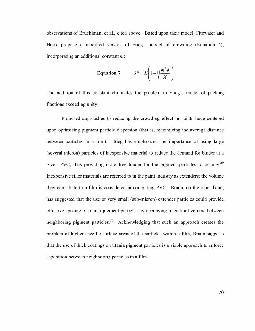
upon optimizing pigment particle dispersion (that is, maximizing the average distance

between particles in a film). Stieg has emphasized the importance of using large

(several micron) particles of inexpensive material to reduce the demand for binder at a

given PVC, thus providing more free binder for the pigment particles to occupy.29

Inexpensive filler materials are referred to in the paint industry as extenders; the volume

they contribute to a film is considered in computing PVC. Braun, on the other hand,

has suggested that the use of very small (sub-micron) extender particles could provide

effective spacing of titania pigment particles by occupying interstitial volume between

neighboring pigment particles.25 Acknowledging that such an approach creates the

problem of higher specific surface areas of the particles within a film, Braun suggests

that the use of thick coatings on titania pigment particles is a viable approach to enforce

separation between neighboring particles in a film.

21

Figure 3. The scattering coefficient S* for rutile titania particles in a typical paint film as a function of pigment volume concentration. (After Braun25)

2.2.2.2 Light Scattering in Stereolithography

This discussion of light scattering by concentrated particle dispersions has

focused entirely upon pigmented paint films; it is in this field where the most extensive

characterization of the optics of concentrated dispersions has occurred historically.

Recently, there has been a rapid growth in interest in the behavior of concentrated

ceramics dispersions in photopolymer solutions. In stereolithography, complex

geometries are formed by ultraviolet laser exposure of a ceramic particle slurry in a

photosensitive solution. Exposure by the laser causes the solution to polymerize, and

the laser position is controlled very accurately by computer. Generation of three-

dimensional shapes is possible since the laser scans with two degrees of freedom in the

x-y plane and the slurry bath can be translated in the z direction. The geometry of a

22

stereolithography apparatus is shown in Figure 4. Once a three-dimensional geometry

is formed, the part is fired to burn out the polymer and form a dense ceramic.

A critical issue in stereolithography is control of the exposure depth of the laser

into the ceramic particle slurry; prediction of this depth requires an understanding of its

dependence upon such factors as laser power, laser dose, laser wavelength, the

refractive index of the ceramic particles, the volume concentration of ceramic particles,

and ceramic particle size. The relationship between cure depth Dc and the scattering

coefficient S* of the particles (neglecting absorption) is:

Equation 8

=

cc E

ES

D 0ln*1

φ

where φ is the volume fraction of particles, E0 is the exposure energy of the laser at the

surface of the suspension, and Ec is the critical exposure energy required to polymerize

the monomer solution. In 1997, Griffith and Halloran performed a series of model

experiments using alumina and silica particles in UV curable solutions and proposed the

following empirical form of the cure depth in concentrated dispersions:30

Equation 9

∆

=c

c EE

nn

sdD 0

2

20 ln

32 λ

where d is the average particle diameter, λ is the laser wavelength in the photopolymer

medium, s is the average surface-to-surface interparticle spacing in the medium, n0 is

the refractive index of the medium, and ∆n is the difference in refractive index between

the particles and the medium. Equation 9, when written in the form used above in the

case of paint films, is:

23

Equation 10 3*φφXKS =

where K is a constant (containing λ, n0 and ∆n). Equation 10 exhibits the obvious

problem of diverging to infinity as φ approaches zero. While Equation 9 apparently

provides a reasonable fit to the limited data of Griffith and Halloran, this relation cannot

apply to systems exhibiting wide variations in the parameters contained in the

expression.

Figure 4. Schematic diagram of a stereolithography apparatus for producing complex ceramic parts using rapid prototyping. (After Liao.31)

2.2.3 Light Scattering by Particle Agglomerates

2.2.3.1 Computational Approaches

During the past three decades, there has been considerable progress in the

experimental and rigorous theoretical understanding of the light scattering behavior of

24

multiple-particle agglomerates or clusters. Spherical particles have been by far the most

extensively investigated particle shape, owing to the availability of analytical

expressions for radiation scattering by a single sphere from Mie theory. In this case, the

light scattered by one sphere in the cluster is decomposed into a series expansion of

outgoing spherical waves which, in turn, impinge upon the other spheres in the cluster.

The field incident upon any sphere in the cluster is therefore a superposition of the total

incident field and scattered fields from all of the other particles in the cluster.

Coefficients coupling the multipole modes in one sphere to those in every other sphere

in the system appear explicitly in the solution. Solution of the problem requires

overcoming the challenge of representing the spherical waves about any sphere in the

cluster as an expansion about any other arbitrary origin. The addition theorems for

spherical vector wave functions in integral form which produce the required translation

coefficients were established by Stein32 and Cruzen33 in the early 1960s. In 1971,

Bruning and Lo published the first comprehensive solution for a two-sphere cluster.34,35

In 1988, the order-of-scattering approach was developed by Fuller and Kattawar, who

extended Bruning and Lo’s solution to the case of larger clusters by considering

pairwise interactions between the constituent spheres. In 1991, Mackowski36 developed

a set of recurrence relations for the translation coefficients which provide a significantly

more efficient computational approach than the integral forms. Borghese, et al., in 1984

were the first to produce expressions for the cross sections of multiple sphere clusters.37

In 1995, Xu derived expressions for both the scattering cross sections and the elements

of the Mueller scattering matrix of multiple-sphere clusters.38 (The Mueller scattering

25

matrix describes changes in polarization of the incident light due to the scattering

interaction.) In 1996, Mackowski and Mishchenko described a T-matrix approach to

the problem of light scattering by sphere aggregates, facilitating computation of the

scattering properties under conditions of random illumination. Fuller points out that the

convergence rate of the solution for a multiple-sphere cluster depends upon the

maximum spacing between a pair of spheres in the cluster, resulting from additional

terms required to compute accurately the translation terms required to transform

multipole coefficients from one sphere location in the cluster to another.39

2.2.3.2 Computational Results for Particle Agglomerates

Computational results for multiple-sphere clusters have been limited, with most

of the activity in the literature focusing upon the development of more computationally

efficient methods as opposed to the application of those methods. Borghese, et al.,37

present computed results on the scattering cross sections of two-sphere systems as a

function of illumination direction and sphere separation distance. For even the largest

sphere separation distances studied (200 sphere diameters), the scattering cross section

of the two-sphere system failed to converge to the sum of the cross sections of the two

independent spheres. The explanation for this observation is that the spheres studied in

this work were very small compared to the radiation wavelength, corresponding to the

Rayleigh scattering limit. While the maximum sphere separation distance studied was

very large compared to the sphere diameter, this distance was smaller than the light

wavelength, causing the two particles to behave like a single Rayleigh scatterer with

twice the volume of the individual spheres. It can be stated, in general, that deviations

26

in the optical behavior of an ensemble of spheres from the behavior of the isolated

spheres as a function of interparticle separation (expressed in diameters of the spheres)

will be greatest for small particles. This is consistent with the experimental

observations of Bruehlman, et al.,26 and the predictions of Stieg27 and Fitzwater and

Hook28 for crowded paint systems. In their computations on touching, slightly

absorbing two-sphere clusters, Mishchenko, et al.,40 reported that two randomly

oriented spheres with diameters greater than one wavelength can become effectively

independent scatterers at surface-to-surface separations as small as one sphere diameter;

this is not the case for spheres with size smaller than the incident wavelength. Fuller39

has observed that the scattering cross sections of two touching spheres which are each

large compared to the wavelength rapidly approach those of the independent spheres

with increasing separation, provided that one particle is not in the shadow of the other.

If shadowing effects are significant, Fuller reports that the cross sections may deviate

from those of the independent sphere by 5−10% for separations as large as 25

diameters.

Approximate methods which have been applied to the study of light scattering

by particle agglomerates include geometrical optics models (Section 2.3.3.2), which are

limited to the case where the primary particle size is substantially greater than the light

wavelength, and coupled-dipole models (Section 2.3.3.4), which are limited to the case

where the primary particles are substantially smaller than the light wavelength.

Geometrical optics models have been applied to the study of light scattering by ice

crystal agglomerates41 and fractal agglomerates of spheres.42 The coupled-dipole

27

method (Section 2.3.3.5) has been applied to the study of light scattering by fractal

agglomerates.43

2.3 Principles of Light Scattering

The phenomenon of electromagnetic radiation scattering is governed by

Maxwell’s equations, a set of physical laws which provides a rigorous basis for the

mathematical description of classical wave propagation. Their validity appears to be

universal, applying to all interactions between electromagnetic energy and matter. The

historic development of the physics underlying Maxwell’s equations can be found in

virtually any elementary physics text. Maxwell’s equations are described in Section

2.3.1. Exact, analytical solutions to Maxwell’s equations for different scattering

geometries are described in Section 2.3.2. Finally, a variety of approximate and

numerical solutions of light scattering are described in Section 2.3.3.

2.3.1 Maxwell’s Equations

Maxwell’s equations are two partial differential equations relating the five

vector quantities B, E, D, J, and H. These are magnetic induction, electric field

intensity, electric displacement, current density, and magnetic field intensity,

respectively. These two equations are:

Equation 11 EtB

×∇=∂∂

−

Equation 12 HJtD

×∇=+∂

∂

28

The set of three constitutive equations which interrelate these five vector quantities

make this pair of differential equations determinate. The constitutive relations for

isotropic materials are:

Equation 13 HB µ=

Equation 14 ED ε=

Equation 15 EJ σ=

where µ is the magnetic permeability, ε is the dielectric permeability, and σ is

conductivity. In the case of anisotropic materials, these three scalars are replaced by

tensors. Substituting the constitutive relations into the partial differential equations in

Equation 11 and Equation 12 and eliminating B, D, and J yields the following

determinate pair of Maxwell’s equations in E and H:

Equation 16 EtH

×∇=∂

∂− µ

Equation 17 HEtE

×∇=+∂∂ σε

Eliminating H between these two equations with the assumption that µ is not a function

of position (which is the case in non-magnetic materials) yields the second order partial

differential equation in E:

Equation 18 EtE

tE

×∇×∇−=∂∂

+∂∂

µσε 1

2

2

This equation is a point form of Maxwell’s equations, meaning that it is valid at a

mathematical point in space, within an arbitrary material. It is the basis for time-

29

domain solutions to scattering problems using Maxwell’s equations. Below, in the

description of the finite element approach, this point form is elaborated into an integral

form which facilitates numerical solution of this equation throughout an extensive

three-dimensional volume.

In Equation 16 and Equation 17, the time dependence of electric field is

expressed explicitly. In general, the steady-state radiation scattering properties of a

body are of interest; only in cases with time-varying materials properties or fields are

variations in scattering properties of direct interest. It is therefore useful to express the

time dependence of Maxwell’s equations implicitly rather than explicitly. To

accomplish this, electric and magnetic field are represented as phasors. In the case of

electric field, for example, this representation has the form:

Equation 19 }),,(Re{),,,( tiezyxEtzyxE ω=

where ω is the angular frequency of the propagating electromagnetic wave. Equation

18 can therefore be rewritten as:

Equation 20 EEiE ×∇×∇−=+−µ

ωσεω 12 .

The vector identity:

Equation 21 ( ) EEE 2∇−⋅∇∇=×∇×∇

in conjunction with the fact that, with no free charges present,

Equation 22 0=⋅∇ E

can be used to rewrite Equation 20 as:

30

Equation 23 EEiE 22 1∇=+−

µωσεω .

This is the Helmholtz equation for electric field expressed implicitly with respect to

time. This equation is the starting point for frequency-domain solutions to scattering

problems using Maxwell’s equations.

2.3.2 Exact, Analytical Solutions of Light Scattering

Of interest in this dissertation is the study of light scattering by complex

materials microstructures, with most of this work focusing upon the light scattering

behavior of systems containing complex single scattering features or multiple features

which exhibit near-field optical interactions. Even in ensembles of multiple scattering

features where the assumption of single scattering is violated, the scattering properties

of single particles remain the starting point for analysis. The subject of single scattering

has therefore received a great deal of attention, with comprehensive surveys presented

by Bohren and Huffman,1 van de Hulst,2 and Kerker.44

The development of exact, analytical solutions to Maxwell’s equations for

electromagnetic radiation scattering by isolated, three-dimensional bodies is possible in

cases where the surfaces of these bodies correspond to coordinate surfaces of coordinate

systems in which the solution to the scalar wave equation:

Equation 24 022 =+∇ ψψ k

is separable. This has been accomplished in the cases of an infinite circular right

cylinder,45,46 an infinite elliptical right cylinder,47 a sphere,48 and an ellipsoid.49,50,51

31

The solutions for infinite cylinders are of interest in the case of fibers which are very

long compared to their radii. The solution for the case of a sphere is the well-known

Mie theory, named for the German scientist Gustav Mie who presented this solution to

Maxwell’s equations in 1908.48 Mie theory figures centrally in the problem of radiation

scattering by any isolated particle which can be reasonably approximated as a sphere

and has therefore been widely applied in diverse fields where scattering by particles is

of interest. Owing to its importance, a survey of this theory is presented below.

Solutions for the case of an ellipsoid involve computational effort which is far more

intensive than that required for a sphere, compounded by the necessity of averaging

over all orientations of the particle relative to the incident radiation, and application of

these solutions has therefore not become commonplace.1 It should be noted that

separation of variables can also be applied to systems in which the optical properties

vary with diameter. This has been accomplished for the case of a sphere52,53,54 and an

infinite right cylinder.55,56,57 In this way, systems with coatings or radial segregation of

materials can be rigorously treated.

Clear and detailed developments of the mathematical treatments underlying Mie

theory are presented by Bohren and Huffman,1 van de Hulst,2 and Kerker.44 Given an

isotropic, spherical particle of arbitrary radius and optical properties illuminated by

electromagnetic radiation of arbitrary wavelength, of interest are the scattered fields

from this particle at far field (i.e., at a position located many wavelengths away from the

particle). The relationship between the electric field vectors associated with the

incident (Ei ) and scattered (Es) electromagnetic waves is required. The first step in this

32

development is to identify a pair of vector harmonics, both of which satisfy the vector

wave equation, generated from the scalar function ψ in Equation 24. These vector

harmonics M and N are of the form:

Equation 25 )( ψrM ×∇=

Equation 26 k

MN )(×∇=

where r is an arbitrary constant vector. As required for an electromagnetic field, both

M and N are divergence-free and satisfy the vector wave equation:

Equation 27 022 =+∇ AkA ,

provided ψ is a solution to the scalar wave equation. The scalar wave equation can be

rewritten in spherical coordinates and ψ represented as the product of three functions,

each a function of just one of the spherical coordinate system variables r, φ, and θ. This

accomplished, the vector spherical harmonics M and N are generated from ψ. The next

step is to represent the incident plane wave as an infinite series with the vector spherical

harmonics as basis functions. Finally, by imposing boundary conditions dictated by

Maxwell’s equations for the tangential components of electric and magnetic field at the

surface of the sphere, the incident and scattered fields outside the sphere can be related

in a series expansion employing a pair of determinate scattering coefficients an and bn.

The forms of these scattering coefficients and the implementation of Mie theory in

computer code are described in Chapter 3.

33

2.3.3 Approximate and Numerical Solutions of Light Scattering

It is often true that the geometries of scattering features whose electromagnetic

radiation scattering properties are of interest do not conform to the geometric limitations

imposed by the exact analytical solutions produced by the separation of variables. For

such cases, which may involve irregular particle shapes or dependent scattering effects,

a host of approximate analytical and numerical approaches have been developed to

determine the radiation scattering properties of the system. Rayleigh scattering theory

and geometrical optics are approximate analytical approaches introduced in Chapter 1

which produce simple expressions for the distribution of scattered light and the

scattering efficiency terms. The remainder of the techniques discussed below are

numerical approaches which in general require substantial computational resources.

2.3.3.1 Rayleigh Theory

In the case where the wavelength of electromagnetic radiation interacting with a

particle is much greater than the particle diameter, the incident electric field can be

reasonably approximated as constant throughout the volume of the particle. The

solution of scattering problems under this approximation is termed Rayleigh theory.58

In Rayleigh theory, the particle is presumed to respond to the applied, time-varying

electric field of the radiation as an oscillating dipole which radiates scattered fields in

all directions. The induced dipole moment of the particle is a vector quantity

proportional to the applied electric field through the polarizability α, a tensor. With the

induced dipole moment known, it is straightforward to compute the resulting electric

34

field at an arbitrary point outside the particle. The induced dipole moment has been

determined analytically for a sphere, a coated sphere,2 an ellipsoid,59 and a coated

ellipsoid.1 In addition, anisotropic polarizability can be incorporated into each of these

particle geometries.60 The polarizability of a material is often isotropic, in which case it

can be treated as a scalar. The angular intensity distribution of scattered light for

unpolarized incident radiation is then given by:

Equation 28 ( )02

242

2cos1 I

rkI αθ+

=

where θ is the scattering angle, r is the distance of the observation point from the

particle, I0 is the incident intensity, and

Equation 29 0

2λ

π mednk =

where nmed is the refractive index of the surrounding medium and λ0 is the wavelength

of the incident wavelength in vacuum.

The most fundamental far-field scattering property is the scattering cross

section, defined as the ratio of scattered power to the incident radiation intensity and

expressed in units of area. The scattering cross section of a sphere in the Rayleigh

approximation is given by:

Equation 30 2

2

24

2

21

38

+−

=mmxaCsca

π

35

where a is the particle radius, m is the relative refractive index of the particle (particle

refractive index divided by that of the surrounding medium) and x is the unitless size

parameter:

Equation 31 kax = .

For fixed particle radius in the Rayleigh regime and with the assumption that m is

independent of wavelength, Equation 30 can be used to explain at least partially the

bluish color of the daytime sky, since scattering cross sections associated with shorter

wavelengths (e.g., blue light) exhibit are greater by a factor (λlong/λshort)4 than scattering

cross sections longer wavelengths (e.g., red light).

The qualitative criterion for validity of the Rayleigh approximation is:

Equation 32 1<<xm .

The appearance of both m and x in the validity criterion above arises because even in

the case of a particle which is small compared to the radiation wavelength in the

medium surrounding outside the particle, the compressed wavelength of the radiation

inside the particle could be sufficiently short compared to the particle diameter to

excite, say, quadrapole radiation in addition to the dipole radiation solely assumed in

the Rayleigh approximation.

2.3.3.2 Geometrical Optics

In the case where the size of a particle is very large compared to the radiation

wavelength, the incident wavefront encountering the particle can be approximated as a

group of independent rays. In the geometrical optics approximation, the incident

36

wavefront is divided into rays which encounter the particle directly and rays which pass

along its surface. The scattering problem is treated as a separable combination of

reflection, refraction, and diffraction.61,62 The reflected and refracted rays conform to

the laws of Fresnel and Snell, which determine the fraction of light reflected, refracted,

and transmitted at each boundary of the particle, as depicted in Figure 5. These events

depend intimately upon both the geometry and optical properties of the scattering

particle. In the case of irregularly shaped particles, the computational requirements for

geometrical optics can be intensive. The method is best suited to convex and highly

reflective scattering features; the multiple scattering of rays which can occur in the

cases of concave and transparent particles presents computational difficulties.63 Those

incident rays which pass along the surface of the particle undergo Fraunhofer

diffraction. The Fraunhofer diffraction pattern is intense and strongly forward-directed.

This pattern depends only upon the size and shape of the particle and is independent of

the optical properties of the particle. This non-intuitive fact is based in Babinet’s

principle (1837), which states that the diffraction created by a large particle with

arbitrary optical properties is identical to that created by a hole of the same size cut

from a perfectly opaque screen. The diffracted energy is therefore equal to the sum of

the reflected and refracted energies, and it is for this reason that the scattering cross-

section of any particle in the geometrical optics limit is equal to exactly twice its

geometric cross-section.64

The light intensity at any observation point is determined in the geometrical

optics approximation by summing the ray contributions from different regions of the

37

particle (or ensemble of multiple particles). If the incident wavefront is coherent, the

scattered rays have a regular phase relationship and amplitudes are summed at the

observation point rather than intensities. In the case of ensembles of multiple particles

having a range of particle sizes, phase relationships can be neglected and intensities of

scattered rays are added at the observation point rather than amplitudes.

The qualitative validity criterion for geometrical optics is that the particle size be

much greater than the radiation wavelength:

1>>x .

On a more precise footing, van de Hulst estimates that geometrical optics is valid for

particles which are at least 20 wavelengths in extent.2 For particles smaller than this, it

is difficult to distinguish between rays which are incident upon the particle and those

which pass along its surface. This estimate is in agreement with results comparing the

light scattering properties of hexagonal ice crystals using geometrical optics and a finite

difference time-domain method, for which close agreement is claimed for x > 20.65

38

Figure 5. Schematic diagram showing reflection and refraction of a light ray using the geometrical optics approximation. (After Bohren and Huffman1)

2.3.3.3 Point Matching

The point matching method66,67 can be used to determine the radiation scattering

properties of non-spherical particles of arbitrary size whose shapes are approximately

spherical. In this method, fields inside and outside the particle are expanded in a

truncated series of vector spherical harmonics and the boundary condition requiring that

tangential field components be continuous at the sphere surface is imposed at a number

of points on the surface. This number of points corresponding to the number of

unknowns in the series expansions, resulting in a set of simultaneous linear equations.

This method is conceptually simple but suffers from uncertain convergence and its

limitation to nearly spherical particles.63

2.3.3.4 Perturbation Methods

Perturbation methods,68,69,70,71 like the point matching method, attempt to

determine the radiation scattering properties of particles which deviate from a shape

whose scattering properties are known analytically. The shape of any particle can, in

principle, be viewed as a sphere with a perturbed shape. Perturbation methods represent

the scattering properties of the geometrically perturbed particle as an infinite series in

some perturbation parameter of which the results of Mie theory form the first term.

These methods suffer from the same problem of uncertain convergence as the point

matching method, and the computation of a prohibitive number of terms may be

required before the infinite series may be truncated without appreciable error. It

39

appears that perturbation methods, like the point matching method, are limited to nearly

spherical particles.

2.3.3.5 Coupled-Dipole Method

A scattering object can be approximated as a collection of radiating electric

dipoles which are excited by both the incident electromagnetic radiation and each other.

This is the principle of the coupled-dipole, or discrete-dipole, method. This method was

first developed by DeVoe in 1964 and applied to scattering by molecular aggregates

very small compared to the radiation wavelength.72,73 The method was generalized to

arbitrary size parameters by Purcell and Pennypacker in 1973, who included retardation

effects and applied the method to determine the scattering properties of interstellar

dust;74 the coupled-dipole method is sometimes still referred to as the Purcell-

Pennypacker method. This method has the advantage of ready applicability to arbitrary

geometries without restriction to nearly spherical shapes. In addition, since the

polarizability of a material is a tensor, the coupled dipole method can be used to

compute the scattering properties of anisotropic materials.75 Its accuracy is limited in

principle only by the density of the electric dipole array, which is in turn limited only by

the availability of computational resources.

A critical feature of the coupled-dipole method is the function chosen to relate

the polarizability αj of the discrete dipoles to the dielectric properties of the bulk

material being represented. The Clausius-Mossotti relation provides an exact function

40

for the particular case of an infinite cubic lattice of dipoles in the dc limit, where the

size of the dipoles divided by the radiation wavelength approaches zero:76

Equation 33 ( )( )med

medCM

n εεεε

α2

3+−

=

where ε is the dielectric function of the scattering material, εmed is the dielectric function

of the surrounding medium, and n is the number of discrete dipoles per unit volume.

Numerous schemes for modifying the Clausius-Mossotti relation have been proposed to

improve the accuracy the coupled-dipole method for realistic, finite-sized scattering

geometries by adding a term on the order of (kd2)77,78 or (kd3),77,79 where k = 2πnmed/λ0

and d is the interdipole spacing. Recently, Draine and Goodman80 developed an

expression for polarizability of an infinite array of polarizable points so that the array

exhibits the same dispersion relation as a continuum with dielectric constant ε. Draine

and Flatau81 claimed in 1994 that this representation yields the best accuracy to date of

these expressions for dipole polarizability.

The coupled-dipole method features a square matrix with edge length equal to

the number N of discrete dipoles in the scattering geometry being represented. This

NxN matrix expresses the influence of each of the separate dipoles upon each other.

The computational memory required for this method increases as (N3),81 placing a limit

on the number of dipoles which can be used to represent a scattering geometry and,

therefore, upon the accuracy of the method.

41

2.3.3.6 T-Matrix or Extended Boundary Condition Method

Starting with an integral equation formulation of the scattering problem, the T-

matrix or Extended Boundary Condition Method is a promising technique which can be

used to determine the scattering properties of arbitrarily shaped particles. First

proposed by Waterman in 1965 for the special case of perfectly conducting particles,82

it has continued to be refined and has since been extended to general dielectric

particles,83, including finite cylinders,84 homogeneous ellipsoids,84,85,86 coated

ellipsoids,87 and clusters of dielectric spheres.40,88,89,90

Following here a conceptual development of the T-matrix formulation set forth

by Barber and Yeh,84 the method embodies a series of intuitive steps relying upon the

equivalence theorem, which states that the field scattered by a particle can be

considered the product of initially unknown electric and magnetic surface currents

acting on the surface of the body. The T-matrix approach ultimately defines the fields

internal to the scattering object in terms of the incident field, then the surface currents in

terms of the internal fields, and finally the scattered field in terms of the surface

currents. The incident, internal, and scattered fields are expanded in a series of vector

spherical harmonics with f and g the unknown coefficients of the scattered field. The

result after applying boundary conditions is the linear transition or T-matrix, which

relates the coefficients of the scattered field to the known coefficients a and b of the

incident field:86,91

Equation 34

=

ba

Tgf

42

The elements of the T-matrix are integrals over the surface of the particle which depend

only upon the size, shape and optical properties of the particle. These surface integral

reduce to line integrals for axisymmetric particles, which is why the T-matrix has been

applied almost exclusively to such particles.92 Computationally, application of the T-

matrix method involves linear algebra operations, either matrix inversion or iterative

schemes.88 One advantage of the T-matrix approach is that, once the T matrix is

computed for a particle, it is simple to compute results for arbitrary orientations of that

particle relative to the incident fields. While the T-matrix method can be used to

compute the scattering properties of large volumes, computational requirements

increase dramatically with size parameter and deviation from rotational symmetry.86,93

In addition, numerical instability can arise in T-matrix computations on these lower-

symmetry particles.91

2.3.3.7 Method of Moments

Method of moments techniques embody a number of specific methods, each

based upon the solution of an integral form of Maxwell’s equations. The method of

moments was first implemented for Maxwell’s equations by Harrington in 1968.94 Both

surface and volume integration approaches have been described. Like the coupled-

dipole method, the method of moments is applicable to highly irregularly shaped

objects. Method of moments techniques are well-suited to conductive materials and

homogeneous dielectrics, but the implementation becomes cumbersome for

inhomogeneous bodies and dielectric bodies of large volume.63 The method of

43

moments leads to fully populated matrices and therefore the computer memory required

increases rapidly with increasing object size.

In the surface integral formulation of the moment of methods, as in the T-matrix

method, the problem of radiation scattering by an arbitrary body is recast using the

equivalence principle into unknown electric and magnetic surface currents J and M

acting on the body to create the total E and H fields both inside and outside the body.

Electromagnetic boundary conditions are imposed at the surface of the body to relate

the fields inside and outside the body. Following the notation of Medgyesi-Mitschang,

et al.,95 these equivalent surface currents appear in the form of a coupled pair of integral

equations which have the form:

Equation 35 tan21tan21tan )()()()()( rMKKrJLLrEinc

+−+=

Equation 36 tan222

121

tan21tan )(11)()()( rMLLrJKKrHinc

+++=

ηη

where r is the field point on the surface, L and K are known integral operators, the

superscript inc indicates the incident field, and the subscripts 1 and 2 denote regions

outside and inside the body, respectively. The equivalent currents on the surface of the

body are expanded in a set of basis functions fn spanning the surface and substituted into

the pair of equations above. Next, the complex inner product is formed with these

equations, transforming the integral operators L and K into matrix operators. In the

Galerkin form of the method of moments solution, the complex conjugates of fn are

chosen as the testing functions on the surface, and the inner products are formed

44

between the testing functions and the integral equations. The result is a set of linear

equations which are solved to determine J and M. In the determination of the scattering

properties of an arbitrarily shaped body, the surface is represented as a mesh of, say,

triangular elements, and J and M are expanded in terms of a testing function along each

element edge.96

A volume integral formulation of the method of moments described by Hage, et

al., has been applied to inhomogeneous dielectric materials of irregular shape.97 In their

approach, a solid of arbitrary shape is represented as a volumetric mesh of N cubic

elements, with constant electric field assumed in each cell. The mathematical basis of

this approach is to represent Maxwell’s equations in E as the (exact) volume integral

taken over the volume V of the body:

Equation 37 [ ]∫∫∫ −+=V

incrdrrGrErmkrErE 2

32122

22

11 ),()(1)(4

)()(π

where r1 is the point of observation, r2 is a point inside the body, m is the complex index

of refraction of the body, and G is the divergence-free Green’s dyadic for the vector

time-independent form of Maxwell’s equations in E. Discretization of the volume V

into a set of N cubic elements makes this integral equation approximate and creates a

system of 3N linear equations with 3N unknowns, the electric field components in each

element. The time required for a computation increases as (N2), which is the chief

disadvantage of this technique. To their credit, Hage, et al., supplement their derivation

of the volume integral form of Maxwell’s equations with microwave scattering

45

experiments on the same arbitrary shaped modeled computationally; good agreement

between calculation and experiment was established.

2.3.3.8 Finite Difference Time-Domain Method

In the finite difference time-domain approach, Maxwell’s equations are solved

numerically in their differential form. This approach is suitable for determining the

radiation scattering properties of arbitrary structures. In the usual finite difference time-

domain method, a three-dimensional Cartesian model is constructed which consists of

the scattering structure of interest and the surrounding medium. It is possible to

implement other coordinate systems with the finite difference approach, but the

Cartesian system affords by far the greatest flexibility in accommodating irregular

geometries. The model is discretized into a large number of rectangular solid mesh

cells, and appropriate optical properties are assigned to each cell. Absorbing or

radiating (in which only the scattered component of radiation is absorbed) boundary

conditions are assigned to the six outer faces of the model. Incident radiation

propagates through the model in the time domain, and the computation is allowed to

proceed until convergence to steady state is achieved.

The differential equations for E and H solved in the finite difference time

domain approach are the same as those given in Equation 16 and Equation 17:

Equation 38 EtH

×∇=∂

∂− µ

Equation 39 HEtE

×∇=+∂∂ σε

46

The spatial and temporal derivatives appearing in these coupled equations are

represented approximately at any point in the mesh between time steps n and (n+1)

using an approximate difference expression. In the scheme proposed by Kunz and

Luebbers,98 for example, this differencing scheme is explicit and first-order accurate:

Equation 40 t

EEt

Ennn

∆−

≈∂

∂++ 11

Of course, more accurate schemes can be employed, as can more reliably stable,

implicit schemes. Values of E and H are computed at the nodes or centers of the mesh

cells. Accuracy considerations in the finite difference time domain approach are

analogous to those encountered in the coupled-dipole method and the volume integral

formulation of the method of moments, for example: accuracy is controlled in large part

by the density of the finite difference mesh, which is in turn limited by computational

resources. In the scheme proposed by Kunz and Luebbers, there is no storage of a large

matrix, and the memory requirement increases as (N4/3), where N is the number of mesh

cells in the model. This is a considerable advantage over the couple dipole-method and

the volume integral formulation of the method of moments, which exhibit a (N3)

dependency. Another advantage of the finite difference time-domain approach is that it

produces full near-field solutions through the volume of the model, which can be of

considerable interest; this is not the case in the surface integral formulation of the

method of moments, for example. Disadvantages of the finite difference time domain

approach include the inability to represent exactly any skewed surfaces in a model using

the Cartesian mesh cells, the fact that user intervention is required to identify the steady

47

state solution, the errors introduced by the approximate boundary conditions, and the

necessity of transforming the near-field results to far-field results in an additional

computational step. These same considerations arise in the finite element time-domain

approach used in the present research; many of these issues are addressed in more detail

in Chapter 3.

2.2.3.9 Finite Element Method

Finite element methods in electromagnetics are based upon the solution of an

integral form of Maxwell’s equations. In any finite element approach,99 the governing

differential equation is multiplied by an arbitrary weighting or testing function, and this

product is integrated over the entire volume of the computational space of interest. This

computational space is discretized into a large number of volume elements, the size and

shape of which are dictated by the level of accuracy required and the geometry of the

features contained in the volume. The total field is then approximated within each

element by an arbitrary shape function which interpolates between field values at

element nodes or edges. The only restriction on the weighting and shape functions is

that they be of sufficiently high order to be differentiable according to the integral form

of the governing differential equation. The computational volume is truncated using

boundary conditions which attempt to minimize spurious reflection of radiation back

into the volume. The system of volume elements is assembled into a global, NxN

matrix K which multiplies the vector of unknown field values a at each element node or

edge to form the known vector f derived from boundary conditions:

Equation 41 [ ]{ } { }faK =

48

The finite element approach thus yields a system of linear equations which can be

solved for the field throughout each volume element. In the commonly employed

Galerkin formulation, the shape and weighting functions are chosen to be the same

yielding a symmetric K matrix. The matrix K is sparse, yielding a computational

memory requirement which increases as N.100

In frequency-domain finite element approaches to Maxwell’s equations,100,101

the time independent form of Maxwell’s equations is employed. Equation 23, for

example, therefore takes the form:

Equation 42 0'''1 22 =

⋅+⋅−⋅∇−∫∫∫ dVEEiEEEE

V

ωσεωµ

where E' is the weighting or testing function, and this scalar integral equation would be

solved throughout the discretized computational volume V to yield the system of linear

equations in the unknown vector E.

In the present research, the EMFlex software, a versatile finite element time-

domain implementation of Maxwell’s equations, is employed. The EMFlex software

has previously been applied to a number of systems of practical interest, including the

determination of light scattering properties of features on silicon wafers102 and

evaluation of the performance of integrated optical devices103 and waveguides.104,105,106

The implementation of this code is described in Chapter 3. Advantages of the time-

domain approach used in EMFlex over frequency domain approaches include the use of

an efficient, explicit forward integration scheme which requires minimal computer

memory, a robust and stable path to the steady-state solution, and easy extension to

49

include time-dependent optical properties of materials in the system or transient

phenomena such as pulsed beams.107

1 B.E. Warren, X-Ray Diffraction, Dover Publications, Inc., New York (1990). 2 T. Allen, Particle Size Measurement, Chapman and Hall, London (1990). 3 J.H. Braun, A. Baidins, and R.E. Marganski, “TiO2 Pigment Technology: A Review,” Prog. Organic Coat., 20, 105-138 (1992). 4 T.C. Patton, Pigment Handbook, Vol. I, II, and III, John Wiley and Sons, New York (1973). 5 D.P. Fields, R.J. Buchacek, J.G. Dickinson, “Maximum TiO2 Hiding Power − The Challenge,” J. Oil Colour Chem. Assoc., 2, 87-93 (1993). 6 M. Buerger, Elementary Crystallography, John Wiley and Sons, New York (1978). 7 D.C. Cronemeyer, “Electrical and Optical Properties of Rutile Single Crystals,” Phys. Rev., 87 (5), 876-886 (1952). 8 W.L. Bond, J. Appl. Phys., 36, 1874 (1965). 9 K.M. Glassford and J.R. Chelikowsky, “Structural and Electronic Properties of Titanium Dioxide,” Phys. Rev. B, 46 (3), 1284−1298 (1992). 10 D.C. Sayle, C.R.A. Catlow, M.-A. Perrin, and P. Nortier, “Computer Simulation of the Defect Chemistry of Rutile TiO2,” J. Phys. Chem. Solids, 56 (6), 799-804 (1995). 11 S.-D. Mo and W.Y. Ching, “Electronic and Optical Properties of Three Phases of Titanium Dioxide: Rutile, Anatase, and Brookite,” Phys. Rev. B, 51 (19), 13023−13032 (1995). 12 K.M. Glassford and J.R. Chelikowsky, “Optical Properties of Titanium Dioxide in the Rutile Structure,” Phys. Rev. B, 45 (7), 3874-3877 (1992). 13 M.W. Ribarsky, Handbook of Optical Constants, E. D. Palik, ed., Academic Press, New York, (1985). 14 R. Sanjines, H. Tang, H. Berger, F. Gozzo, G. Margaritondo, and F. Levy, “Electronic Structure of Anatase TiO2 Oxide,” J. Appl. Phys., 75 (6), 2945-2951 (1994). 15 H. Tang, H. Berger, P.E. Schmid, and F. Levy, “Optical Properties of Anatase (TiO2),” Solid State Communications, 92 (3), 267-271 (1994). 16 Z. Schroder, "Beitrage zur Kenntnis des Feinbaues des Brookits und des physikalischen Verhaltens sowie Zustandsanderungen der drei naturlichen Titandioxyde," Kristallographie, 67, 542 (1928). 17 W.D. Ross, “Theoretical Computation of Light Scattering Power: Comparison Between TiO2 and Air Bubbles,” J. Paint Technol., 43, 50-66 (1971). 18 B.R. Palmer, P. Stamatakis, C.F. Bohren, and G.C. Salzman, “A Multiple Scattering Model for Opacifying Particles in Polymer Films,” J. Coat. Technol., 61, 41-47 (1989). 19 P. Kubelka and F. Munk, Z. Tech. Physik, 12, 593 (1931). 20 P. Kubelka, J. Opt. Soc. Am., 38, 448 (1948). 21 D.B. Judd and G. Wyszecki, Color in Business, Science, and Industry, Second Edition, John Wiley and Sons, New York, pp. 381-399 (1963).

50

22 W.P. Hsu, R. Yu, and E. Matijevic, “Paper Whiteners, I. Titania Coated Silica,” J. Colloid Interface Sci., 156, 56-65 (1993). 23 United States Patent 5,248,556, “Synthetic Whitener Agent,” Issued to E. Matijevic, P. Hsu, and M.R. Kuehnle. 24 International Patent Application PCT/SE94/00202, “Pigments Having Good Scattering Properties and Process for the Production Thereof,” Applicant: Kompopigment Ltd. 25 J.H. Braun, “Crowding and Spacing of Titanium Dioxide Pigments,” J. Coat. Technol., 60 (758), 67-71 (1988). 26 R.J. Bruehlman, L.W. Thomas, and E. Gonick, “Effect of Particle Size and Pigment Volume Concentration on Hiding Power of Titanium Dioxide,” Official Digest of the Federation of Societies for Paint Technology, 1-16 (1961). 27 F.B. Stieg, “The Effect of Extenders on the Hiding Power of Titanium Pigments,” Official Digest, 31 (408), 52-64 (1959). 28 S. Fitzwater and J.W. Hook, “Dependent Scattering Theory: A New Approach to Predicting Scattering in Paints,” J. Coat. Technol., 57 (721), 39-47 (1985). 29 F.B. Stieg, “Effect of Extender on Crowding of Titanium Pigment,” J. Coat. Technol., 61 (778), 67-70 (1989). 30 M.L. Griffith and J.W. Halloran, “Scattering of Ultraviolet Radiation in Turbid Suspensions,” J. Appl. Phys., 81 (6), 2538-2546 (1997). 31 H. Liao, Stereolithography Using Compositions Containing Ceramic Powders, Doctoral Dissertation, University of Toronto, 1997. 32 A. Stein, “Addition Theorems for Spherical Wave Functions,” Q. Appl. Math., 12, 13-23 (1961). 33 O.R. Cruzan, “Translational Addition Theorems for Spherical Vector Wave Functions,” Q. Appl. Math., 20, 33-40 (1962). 34 K.A. Fuller and G.W. Kattawar, “Consummate Solution to the Problem of Classical Electromagnetic Radiation Scattering by Ensembles of Spheres. I. Linear Chains,” Opt. Lett., 13, 90-92 (1988). 35 K.A. Fuller and G.W. Kattawar, “Consummate Solution to the Problem of Classical Electromagnetic Radiation Scattering by Ensembles of Spheres. II. Clusters of Arbitrary Configurations,” Opt. Lett., 13, 1063-1065 (1988). 36 D.W. Mackowski, “Analysis of Radiative Scattering for Multiple Sphere Configurations,” Proc. R. Soc. London Ser. A, 433, 599-614 (1991). 37 F. Borghese, P. Denti, R. Saija, G. Toscano, and O.I. Sindoni, “Multiple Electromagnetic Scattering from a Cluster of Spheres. I. Theory,” Aerosol Sci. Technol., 3, 227-235 (1984). 38 Y. Xu, “Electromagnetic Scattering by an Aggregate of Spheres,” Appl. Opt., 34 (21), 4573-4588 (1995). 39 K.A. Fuller, “Scattering and Absorption Cross Sections of Compounded Spheres. I. Theory for External Aggregation,” J. Opt. Soc. Am. A, 11 (12), 3251-3260 (1994). 40 M.I. Mishchenko, D.W. Mackowski, and L.D. Travis, “Scattering of Light by Bispheres with Touching and Separated Components,” Appl. Opt., 34 (21), 4589-4599 (1995). 41 A. Macke, “Scattering of Light by Polyhedral Ice Crystals,” Appl. Opt., 32, 2780-2788 (1993).

51

42 R. Jullien and R. Botet, “Light Scattering by Fractal Aggregates: A Monte-Carlo Method in the Geometrical Optics Limit,” J. Phys. France, 50, 1983-1994 (1989). 43 J. Frey, J.J. Pinvidic, R. Botet, and R. Jullien, “Light Scattering by Fractal Aggregates: A Numerical Investigation,” J. Phys. France, 49, 1969-1976 (1988). 44 M. Kerker, The Scattering of Light and Other Electromagnetic Radiation, Academic, New York, (1969). 45 R.F. Harrington, Time-Harmonic Electromagnetic Fields, McGraw-Hill, New York, 1961. 46 J.R. Wait, “Scattering of a Plane Wave from a Circular Dielectric Cylinder at Oblique Incidence,” Can. J. Phys., 33, 189-195 (1955). 47 C. Yeh, “Scattering of Obliquely Incident Light Waves by Elliptical Fibers,” J. Opt. Soc. Am., 54, 1227-1231 (1964). 48 G. Mie, "Beitrage zur Optik Truber Medien Speziell Kolloidaler Metallosungen", Ann. Phys., 25, 377-445, (1908). 49 S. Asano and G. Yamamoto, “Light Scattering by a Spheroidal Particle,” Appl. Opt., 14, 29-49 (1975). 50 S. Asano, “Light Scattering Properties of Spheroidal Particles,” Appl. Opt., 18, 712-723 (1979). 51 S. Asano and M. Sato, “Light Scattering by Randomly Oriented Spheroidal Particles,” Appl. Opt., 19, 962-974 (1980). 52 A.L. Aden and M. Kerker, “Scattering of Electromagnetic Waves from Two Concentric Spheres,” J. Appl. Phys., 22, 1242-1246 (1951). 53 R.L. Hightower, and C.B. Richardson, “Resonant Mie Scattering from a Layered Sphere,” Appl. Opt., 27, 4850-4855 (1988). 54 P.J. Wyatt, “Scattering of Electromagnetic Plane Waves from Inhomogeneous Spherically Symmetric Objects,” Phys Rev., 127, 1837-1843 (1962). And Errata, Phys. Rev., 134, AB1 (1964). 55 A.W. Adey, “Scattering of Electromagnetic Waves by Coaxial Cylinders,” Can. J. Phys., 34, 510-520 (1956). 56 M. Kerker and E. Matijevic, “Scattering of Electromagnetic Waves from Concentric Infinite Cylinders,” J. Opt. Soc. Am., 51, 506-508 (1961). 57 W.A. Farone and C.W. Querfield, “Electromagnetic Radiation Scattering from Radially Inhomogeneous Infinite Cylinders at Oblique Incidence, J. Opt. Soc. Am., 56, 476-480 (1966). 58 Lord Rayleigh, Phil. Mag., 41, 107, 274, and 447 (1871). 59 Lord Rayleigh, Phil. Mag., 44, 28 (1897). 60 R. Clark Jones, Phys. Rev., 68, 93 and 213 (1945). 61 J.B. Keller, “Geometrical Theory of Diffraction,” J. Opt. Soc. Am., 52 (2), 116-130, 1962. 62 J.R. Hodkinson and I. Greenleaves, “Computations of Light-Scattering and Extinction by Spheres According to Diffraction and Geometrical Optics, and Some Comparisons with the Mie Theory,” J. Opt. Soc. Am., 53 (5), 577-588 (1963).

52

63 C. Yeh and K.K. Mei, “On the Scattering from Arbitrarily Shaped Inhomogeneous Particles − Exact Solution,” in Scattering by Irregularly Shaped Particles, ed. D. Schuerman, Plenum, New York, 201-206 (1980). 64 O. Struve, Ann. Astrophys., 1, 143 (1938). 65 P. Yang and K.N. Liou, “Light Scattering by Hexagonal Ice Crystals: Comparison of Finite Difference Time Domain and Geometric Optics Models,” J. Opt. Soc. Am. A, 12 (1), 162-176 (1995). 66 T. Oguchi, “Attenuation and Phase Rotation of Radio Waves Due to Rain: Calculations at 19.3 and 34.8 GHz,” Radio Sci., 8, 31-38 (1973). 67 R.H.T. Bates, “Analytic Constraints on Electromagnetic Field Computations,” IEEE Trans. Microwave Theory Tech., MTT-23, 605-623 (1975). 68 C. Yeh, “Perturbation Approach to the Diffraction of Electromagnetic Waves by Arbitrarily Shaped Dielectric Obstacles,” Phys. Rev., 135, A1193-A1201 (1964). 69 V.A. Erma, “An Exact Solution for the Scattering of Electromagnetic Waves from Conductors of Arbitrary Shape: I. Case of Cylindrical Symmetry,” Phys. Rev., 173, 1243-1257 (1968). 70 V.A. Erma, “Exact Solution for the Scattering of Electromagnetic Waves from Conductors of Arbitrary Shape: II. General Case,” Phys. Rev., 176, 1544-1553 (1968). 71 V.A. Erma, “Exact Solution for the Scattering of Electromagnetic Waves from Bodies of Arbitrary Shape: III. Obstacles with Arbitrary Electromagnetic Properties,” Phys. Rev., 179, 1238-1246 (1969). 72 H. DeVoe, “Optical Properties of Molecular Aggregates. I. Classical Model of Electronic Absorption and Refraction,” J. Chem. Phys., 41, 393-400 (1964). 73 H. DeVoe, “Optical Properties of Molecular Aggregates. II. Classical Theory of the Refraction, Absorption, and Optical Activity of Solutions and Crystals,” J. Chem. Phys., 43, 3199-3208 (1965). 74 E.M. Purcell and C.R. Pennypacker, “Scattering and Absorption of Light by Nonspherical Dielectric Grains,” Astrophys. J., 186, 705-714 (1973). 75 S.B. Singham and G.C. Salzman, “Evaluation of the Scattering Matrix of an Arbitrary Particle Using the Coupled Dipole Approximation,” J. Chem. Phys., 84 (5), 2658-2667 (1986). 76 H.A. Lorentz, Theory of Electrons, Teubner, Leipzig, (1909). 77 G.H. Goedecke and S.G. O’Brien, “Scattering by Irregular Inhomogeneous Particles Via the Digitized Green’s Function Algorithm,” Appl. Opt., 27, 2431-2438 (1988). 78 C.E. Dungey and C.F. Bohren, “Light Scattering by Nonspherical Particles: a Refinement to the Coupled-Dipole Method,” J. Opt. Soc. Am A, 8 (1), 81-87 (1991). 79 B.T. Draine, “The Discrete-Dipole Approximation and it Application to Interstellar Graphite Grains,” Astrophys. J., 333, 848-872 (1988). 80 B.T. Draine and J. Goodman, “Beyond Clausius-Mossotti: Wave Propagation on a Polarizable Point Lattice and the Discrete Dipole Approximation, Astrophys. J., 405, 685-697 (1993). 81 B.T. Draine and P.J. Flatau, “Discrete-Dipole Approximation for Scattering Calculations,” J. Opt. Soc. Am. A, 11 (4), 1491-1499 (1994). 82 P.C. Waterman, “Matrix Formulation of Electromagnetic Scattering,” Proc. IEEE, 53, 805-812 (1965).

53

83 P.C. Waterman, “Symmetry, Unitarity, and Geometry in Electromagnetic Scattering,” Phys. Rev. D, 3 (4), 825-839 (1971). 84 P. Barber and C. Yeh, “Scattering of Electromagnetic Waves by Arbitrarily Shaped Dielectric Bodies,” Appl. Opt., 14, 2864-2872 (1975). 85 W. Wiscombe and A. Mugnai, “Exact Calculations of Scattering from Moderately-Nonspherical Tn-Particles: Comparisons with Equivalent Spheres,” in Scattering by Irregularly Shaped Particles, ed. D. Schuerman, Plenum, New York, 201-206 (1980). 86 P.E. Geller, T.G. Tsuei, and P.W. Barber, “Information Content of the Scattering Matrix for Spheroidal Particles 87 D.S. Wang and P.W. Barber, “Scattering by Inhomogeneous Nonspherical Objects,” Appl. Opt., 18, 1190-1197 (1979). 88 D.W. Mackowski and M.I. Mishchenko, “Calculation of the T Matrix and the Scattering Matrix for Ensembles of Spheres,” J. Opt. Soc. Am. A, 13 (11), 2266-2278 (1996). 89 D.W. Mackowski, “Calculation of Total Cross Sections of Multiple-Sphere Clusters,” J. Opt. Soc. Am A, 11 (11), 2851-2861 (1994). 90 Y. Xu, “Electromagnetic Scattering by an Aggregate of Spheres,” Appl. Opt., 34 (21), 4573-4588 (1995). 91 M.I. Mishchenko, D.W. Mackowski, and L.D. Travis, “T-Matrix Computations of Light Scattering by Nonspherical Particles: A Review,” J. Quant. Spectrosc. Radiat. Transfer, 55 (5), 535-575 (1996). 92 P.W. Barber and S.C. Hill, Light Scattering by Particles: Computational Methods, World Scientific, Singapore, (1990). 93 A. Mugnai and W.J. Wiscombe, “Scattering from Nonspherical Chebyshev Particles. I: Cross Sections, Single-Scattering Albedo, Asymmetry Factor and Backscattered Fraction,” Appl. Opt., 25, 1235-1244 (1986). 94 R.F. Harrington, Field Computation by Moment Method, MacMillan, New York, (1968). 95 L.N. Medgyesi-Mitschang, J.M. Putnam, and M.B. Gedera, “Generalized Method of Moments for Three-Dimensional Penetrable Scatterers,” J. Opt. Soc. Am. A, 11 (4), 1383-1398 (1994). 96 S.M. Rao, D.R. Wilton, and A.W. Glisson, “Electromagnetic Scattering by Surfaces of Arbitrary Shape,” IEEE Trans. Antennas Propag., AP-30, 409-418 (1982). 97 J.I. Hage, J.M. Greenberg, and R.T. Wang, “Scattering from Arbitrarily Shaped Particles: Theory and Experiment,” Appl. Opt., 30 (9), 1141-1152 (1991). 98 K.S. Kunz and R.J. Luebbers, The Finite Difference Time Domain Method for Electromagnetics, CRC, Boca Raton, (1993). 99 O.C. Zienkiewicz and K. Morgan, Finite Elements and Approximation, Wiley, New York (1982). 100 J.L. Volakis, A. Chatterjee, and L.C. Kempel, “Review of the Finite Element Method for Three-Dimensional Electromagnetic Scattering,” J. Opt. Soc. Am. A, 11, 1422-1433 (1994). 101 L.A. Liebman, Light Scattering by Spherical Particles: a Finite Element Solution to the Maxwell Equations, UMI Dissertation Services, Ann Arbor, (1994). 102 G.L. Wojcik, D.K. Vaughan, and L.K. Galbraith, “Calculation of Scatter from Structures on Silicon Surfaces,” SPIE 1987 Symposium on Microlithography, 74.

54

103 G.L. Wojcik, J. Mould, and L.C. West, “Time-Domain Finite Element Modeling of 3D Integrated Optical Devices,” Integrated Photonics Research Technical Digest, 10, Optical Society of America, March 1993. 104 A.D. Chaudari, Y. Lu, L.C. West, and C. Roberts, “Highly Compact Optical Waveguides with a Novel Pedestal Geometry,” IEEE Photonic Technol. Lett., 7, 526-528 (1995). 105 L.C. West, C. Roberts, J. Dunkel, G. Wojcik, and J. Mould, “Non Uniform Grating Couplers for Coupling of Gaussian Beams to Compact Waveguides,” Integrated Photonics Research Technical Digest, Optical Society of America, 1994. 106 L.C. West, C. Roberts, and E.C. Piscani, “Ultra High Confinement Waveguides for Very Large Scale Integrated Optics (VLSOI) with Three-Dimensional Packaging,” Integrated Photonics Research Technical Digest, Optical Society of America, 1996. 107 G.L. Wojcik, “Theoretical Description of the EMFlex Finite Element Formulation,” unpublished report, 1991.

55

Chapter 3. Computational Methods

This chapter describes the two methods used in this research to compute the

electromagnetic radiation scattering properties of microstructures. The first is Mie

theory (Section 3.1), the second is the time-domain finite element approach (Section

3.2).

3.1 Mie Theory

3.1.1 Computation of the Scattering Coefficients an and bn

The separation of variables approach which underlies the derivation of Mie

theory is described in Section 2.3.2. Here, an elaboration of the mathematical forms of

Mie theory is presented, with emphasis on its implementation into computer code which

can be used to calculate the far-field scattering parameters of interest. In the present

research, Bohren and Huffman’s computer codes BHMIE and BHCOAT are employed

to calculate scattering parameters for homogeneous and coated spheres, respectively.1

Both of these codes have been modified to include computation of the asymmetry

parameter (Section 3.1.2).

Given an isotropic, spherical particle of arbitrary radius and optical properties

illuminated by electromagnetic radiation of arbitrary wavelength, of interest are the

scattered fields from this particle at far field. To this end, the relationship between the

electric field vectors associated with the incident (Ei ) and scattered (Es)

electromagnetic waves must be established. Equation 43 evokes the 2x2 scattering

56

matrix, a mathematical operator which defines the relationship between scattered and

incident radiation at the arbitrary point (x,y,z) located a distance r from the particle.

The incident radiation is assumed to propagate in the +z direction. In general, the

scattering matrix is fully populated, but for the case of a spherical particle, it is

diagonal.1,2

Equation 43 ( )

−

=

−

.,

.,

1

2

.,

.,

00

perpi

parizrik

perps

pars

EE

SS

ikre

EE

.

The subscripts of the electric field vectors refer to polarizations parallel (also called p

polarization) and perpendicular (also called s polarization) to the scattering plane, and

Equation 44 0

.2λ

π mednk = .

In Mie theory computations, the surrounding medium is infinite in extent and therefore

must have zero absorption coefficient; that is, its index of refraction must be a real

number. The values of Sn are given by:

Equation 45 S nn n

a bn

n n n n12 1

1=

++

+∑

( )( )π τ

Equation 46 S nn n

a bn

n n n n22 1

1=

++

+∑

( )( )τ π .

The functions τn and πn are polar functions which depend solely upon the scattering

angle θ. They can be written as simple functions of the Legendre function 1nP :

Equation 47 θ

πsin

1n

nP

= , θ

τddPn

n

1

=

57

The functions τn and πn can be conveniently computed by upward recurrence from the

relations:

( ) 21 1cos

112

−− −−

−−

= nnn nn

nn ππθπ ,

Equations 48 ( ) 11)(cos −+−= nnn nn ππθτ

beginning with π0 = 0 and π1 = 1.

The terms an and bn are the coefficients of the series expansion for the scattered

fields outside the particle. They, like S1 and S2, are generally complex numbers. The

mathematical expressions for these angle-independent scattering coefficients are

complicated but are computed from only upon materials properties and the spherical

Bessel functions ( )xjn and ( ) ( )xhn1 . These expressions are:

Equation 49 am j mx xj x j x mxj mx

m j mx xh x h x mxj mxnn n n n

n n n n

=−

−

µ µµ µ

' ' ' '

21

2 11

1

( ) ( ) ( ) ( )( ) ( ) ( ) ( )( ) ( )

Equation 50 bj mx xj x j x mxj mx

j mx xh x h x mxj mxnn n n n

n n n n

=−

−

µ µµ µ

1

11 1

( ) ( ) ( ) ( )( ) ( ) ( ) ( )( ) ( )

' ' ' '

where µ and µ1 are the permeabilities of the medium and the particle respectively, and

Equation 51 f xx

f x ' ( ) ( )=∂∂

Equation 52 kax =

Equation 53 mednnm 1=

58

where n1 is the real refractive index of the particle. The contrast ratio, m, is the ratio of

the refractive index of the particle to that of the surrounding medium.

The magnitude of the scattered irradiance of a particle as a function of the

scattering angle depends upon the polarization of the incident radiation relative to the

scattering plane. For the case of polarization perpendicular to the scattering plane (i.e.,

the s polarization), scattered irradiance i1 as a function of angle is given by the

expression:

Equation 54 211 )(θSi =

For the case of polarization parallel to the scattering plane (i.e., the p polarization),

scattered irradiance i2 is given by the expression:

Equation 55 222 )(θSi =

The scattered irradiance associated with unpolarized or circularly polarized radiation is

obtained by computing the mean of i1 and i2.

This discussion of Mie theory has focused primarily upon the case of a

homogeneous sphere. These results can be readily extended to the case of an

inhomogeneous sphere consisting of concentric shells with different optical properties.

This is accomplished by expanding the fields within each coating layer in spherical

harmonic basis functions (just as in the solid core of the coated sphere) and imposing

the electromagnetic boundary conditions at both of the interfaces associated with each

coating layer. The result is a modified pair of expressions for the scattering coefficients

59

an and bn outside of the coated sphere, which are functions of the optical properties and

thicknesses of the coating layers.1

3.1.2 Far-Field Scattering Parameters

The most important angle-independent quantity relating to scattering efficiency

of sphere is the scattering cross section, Csca. Scattering cross section is the total power

scattered by the sphere, divided by the incident intensity. It is expressed in units of area.

If one imagines a spherical, mathematical surface with a radius very large compared to

the radiation wavelength and centered at the particle, the scattering cross section can be

visualized as the following surface integral taken over this far-field, mathematical

surface:

Equation 56 0

)(

i

diCsca

∫∫Σ

Σ=

θ

where i(θ) is scattered intensity as a function of scattering angle, dΣ is an infinitesimal

element of surface area, and i0 is the incident intensity. The far-field surface must be a

large distance from the particle to ensure that evanescent fields in the vicinity of the

particle do not reach the far-field surface. The scattering cross section can be computed

from the scattering coefficients as:

Equation 57 ) ( )12(2 22

12 nn

nsca ban

kC ++= ∑

∞

=

π

The scattering cross section can be visualized as the geometric area of the incident plane

wave which is scattered by the particle.

60

In general, the scattering cross section increases with increasing sphere radius.

It is therefore useful to normalize the scattering cross section using the geometric

properties of a particular sphere of interest. One means of normalization is to compute

the ratio of the scattering cross section to the geometric cross section of the sphere. The

result is the unitless scattering efficiency, Qsca:

Equation 58 2aC

Q scasca π

=

The scattering efficiency approaches zero as sphere radius approaches zero and

approaches the value 2 as sphere radius approaches infinity. Between these two limits,

Qsca can in principle attain arbitrarily large values for very high-index particles of

optimal size for strong scattering, though in practice for non-absorbing materials of

physically realistic refractive index, peak values in the resonant regime greater than 2

but less than 10 are observed. The scattering efficiency Qsca is an intuitive quantity

which facilitates comparison of the scattering performance of particles with very

different geometric or physical properties.

It is useful to normalize the scattering cross section in terms of the volume of a

scattering particle. It is more natural on physical grounds to normalize scattering

performance by volume, employing a geometric normalization which is three-

dimensional, than by the two-dimensional cross-sectional area. Paint formulations and

pigment costs, for example, are based upon pigment particle volume rather than upon

particle cross sectional area. Therefore, it useful to evoke a third far-field scattering

61

parameter, the scattering coefficient, S. S is defined as the scattering cross section of a

particle divided by the particle volume:

Equation 59 a

Qa

CS scasca

43

3 4 3

=

=

π

S is expressed in units of inverse length. The reader is cautioned that this S is not the

same quantity as the S* defined for particles or films in the discussion of Kubelka-

Munk theory in Chapter 2.

The asymmetry parameter g is the average cosine of the scattering angle,

weighted by scattered intensity. It is a unitless quantity. The asymmetry parameter

provides important information about the relative importance of forward- and back-

scattering by the spherical particle. Evoking the far-field spherical surface with the

scattering particle at its center described in the case of the scattering cross section, the

asymmetry parameter is defined as:

Equation 60 ∫∫

∫∫

Σ

Σ

Σ

Σ=

di

dig

)(

cos)(

θ

θθ

The asymmetry parameter can be computed from the scattering coefficients an and bn

as:1

Equation 61

where the asterisk denotes the complex conjugate.

62

In the context of multiple scattering, where radiation encounters a large number

of independently scattering particles while traversing an ensemble of such particles, the

asymmetry parameter strongly effects the redirection of scattered radiation and

therefore the scattering efficiency of the ensemble of particles as a whole. The

scattering parameter σ combines the asymmetry parameter and the scattering coefficient

S as follows:

Equation 62 ( )gS −= 1σ

Like the scattering efficiency S, the angle-weighted scattering coefficient σ is expressed

in units of inverse length. In the case of a semi-infinite film containing a large number

of scattering particles, for example, the scattering coefficient σ provides direct

information about how effectively the ensemble back-scatters incident light through

multiple scattering.17,18,2

While it has been assumed in this discussion of far-field scattering parameters

that the scattering particle is a sphere, the quantities Csca, Qsca, S, g, and σ are all equally

well defined for irregularly shaped particles.

3.2 Finite Element Time-Domain Method

The EMFlex time-domain finite element software for solving Maxwell’s

equations is employed in much of the present research. In Section 3.2.1, the basis of its

numerical implementation basis is presented. In Section 3.2.2, details of its application

to problems of interest are described.

63

3.2.1 Numerical Implementation

The following description of the mathematical basis of the EMFlex code follows

closely an unpublished report by Wojcik107, one of the developers of the code. As

described in Section 2.2.3.9, the finite element method allows piece-wise solution of

Maxwell’s equations throughout a discretized computational volume containing

scattering features. The partial differential equation which is solved is the combined

form of Maxwell equations presented in Section 2.3.1:

Equation 63 EtE

tE

×∇×∇−=∂∂

+∂∂

µσε 1

2

2

.

Forming the inner dot product of this equation with the arbitrary vector weighting

function G and integrating over the volume V of the computational volume yields the

integral equation:

Equation 64 ( )dVEGdVtE

tEG

VV∫∫∫∫∫∫ ×∇×∇⋅−=

∂∂

+∂∂

⋅µ

σε 12

2

.

Using a vector identity, the integrand of the right-hand side of Equation 64 can be

rewritten as:

Equation 65 ( ) EGGEEG ×∇×∇−×∇⋅×∇=×∇×∇⋅ .

Substituting Equation 65 into Equation 64 and applying the divergence theorem to the

second term on the right-hand side of Equation 64 gives:

Equation 66

( ) ( )∫∫∫∫∫∫∫∫Σ

Σ×∇×⋅−×∇⋅×∇−=

∂∂

+∂∂

⋅ dEnGdVGEdVtE

tEG

VV µµσε 11

2

2

64

where n is the outward unit vector normal to the surface of the computational volume.

The second order spatial operator appearing in Equation 64 is thus replaced in Equation

66 by first order operators, making numerical implementation of this governing

equation simpler.

The fields E and G are assumed to be separable in time and space, so that:

Equations 67 )()(),( tfxStxE = ; )()(),( tgxStxG =

where the same spatial dependence of the shape function S(x) is assumed for both E and

G. This is the Galerkin formulation in which the weighting and shape functions are

taken to be the same and yields a symmetric system of linear equations in the finite

element formulation. Substituting Equations 67 into the integrands of Equation 66

yields the differential equation:

Equation 68 02

2

=

−−∂∂

+∂∂ fBfK

tfC

tfMg

T

where the superscript T indicates the transpose and

Equation 69 ( )∫∫∫≡V

T dVSSM ε ; ( )∫∫∫≡V

T dVSSC σ ; ( ) ( )∫∫∫ ×∇×∇≡V

T dVSSKµ1 .

K, L, and M are symmetric coefficient matrices, and:

Equation 70 ( )∫∫Σ

Σ×∇×≡ dSnSB T

µ1

is the coefficient matrix defined by the surface integral. Since g(t) is an arbitrary

function, Equation 68 can be rewritten as:

65

Equation 71 ( ) fBKtfC

tfM +=

∂∂

+∂∂

2

2

.

It is this ordinary differential equation which is solved using the finite element approach

by discretizing the computational volume, solving the integral equation within each

element, and constructing the global system of linear equations in the unknown electric

field f(t) at each node in the mesh. Rectangular solid volume elements, with eight

corner nodes, are employed in EMFlex. There are therefore twenty-four unknown

electric field components (three at each node) associated with each element in the finite

element mesh. The interpolating shape function S(x) varies linearly within each

element between the electric field values at each corner. In the time dimension,

EMFlex uses the central difference approximation, which is second-order accurate, to

compute the second derivative with respect to time:

Equation 72 22

2

)()()(2)()(

tttftfttf

ttf

∆∆−+−∆+

≈∂

∂

This is an explicit forward integration scheme.

In EMFlex finite element models, there are several different boundary

conditions which can be assigned to each of the model walls. The absorbing boundary

condition is intended to absorb all incident radiation at the wall, both scattered and non-

scattered. The reflecting boundary condition assigns the properties of a perfect

conductor to a model wall, resulting in complete reflection of all incident radiation.

Symmetric and asymmetric boundary conditions can be used to impart lateral

periodicity to models. Finally, the illumination boundary condition prescribes that only

66

scattered radiation is absorbed at a model wall, allowing non-scattered radiation to pass

through. The illumination and absorbing boundary conditions can contribute to error at

a model wall by causing a measure of spurious reflection of light back into the model.

The illumination boundary condition is used in the finite element models throughout the

present research.

In practice, an individual EMFlex finite element computation results in the

steady-state properties of full electric field quantities (phase and amplitude) in the near-

field surrounding the structure of interest. These near-field quantities can be expressed

in terms of full, scattered, or reflected components. It is necessary to extrapolate these

near-field quantities to far field in a second computational step to extract the far-field

scattering parameters of interest. For this purpose, a mathematical surface (termed the

Kirchoff box) is defined just inside the walls of the finite element model, on which the

equivalent electric and magnetic currents J and M are computed from the tangential

components of scattered electric and magnetic field.45 From these equivalent currents

the scattered electric field at near field is extrapolated onto the surface of a far-field

sphere having a radius which is much greater than the wavelength of light using the

equivalence theorem.45 Extrapolation to far field eliminates evanescent electric field

components which are present at near field so that only propagating electromagnetic

waves contribute to the far-field result. The simulation of diffuse illumination is

accomplished by superimposing the far-field scattered intensities computed from a

series of individual computations in which the illumination directions have been varied

67

step-wise over the full range of necessary orientations. The extrapolation of near-field

intensities to far field is performed using the EMFlex post-processing software, Review.

3.2.2 Use of the EMFlex Software in Practice

The methodology used to run the EMFlex code is straightforward. The platform

used for the EMFlex code is a Cray C-94 supercomputer. The platform used for the

Review code is a Silicon Graphics, Inc. (SGI) Power Challenge mainframe computer.

Individual EMFlex jobs are submitted to the Cray from the SGI in the form of text input

decks. A typical EMFlex input deck is included in the Appendix. The EMFlex input

deck contains parameters defining the geometry of the finite element model, the optical

properties of the materials contained in the model, and parameters defining the

illumination conditions. The geometric parameters of the finite element model include

the physical dimensions of the Cartesian computational space (a rectangular solid in

three-dimensional calculations), the number of finite elements along each edge of the

model, and the size, shape, and position of particles embedded within the model. The

illumination conditions include the free-space wavelength of the illuminating plane

wave radiation, its propagation direction, its amplitude, and its polarization, along with

the boundary condition implemented at each wall of the model.

Upon completion of a run on the Cray, a binary data block containing all of the

user-requested near-field quantities (such as electric field amplitude, phase, and

scattered intensity) is returned to the SGI for subsequent post processing. This post-

68

processing typically includes extrapolation of near-field intensities to the surface of a

far-field sphere and computation of the far-field scattering parameters.

3.2.3 Computation of Far-Field Scattering Parameters

The computation of the scattering cross section Csca and the asymmetry

parameter g for a given microstructure using EMFlex is accomplished by numerical

summations of scattered intensities on the surface of the far-field sphere. In practice the

surface of this far-field sphere is discretized into j surface area elements delineated by a

spherical coordinate system with a user-defined mesh density in the two spherical

angles phi and theta. In these computations, there is an established relationship between

the spherical coordinate system of the far-field surface and the Cartesian coordinate

system of the finite element model. The scattering cross section of a given

microstructure is given by:

Equation 73 0

)(

i

iC j

jj

sca

∑ ∆Σ⋅=

θ

where θ is the scattering angle, i(θj) is the scattered intensity within surface element j,

∆Σj is the surface area of the surface element j, and i0 is the incident radiation intensity

in the finite element computation. The discretized expression in Equation 73 for the

scattering cross section is analogous to the continuum expression given in Equation 56.

The asymmetry parameter g is computed numerically on the surface of the far-

field sphere through the summation:

69

Equation 74 ∑

∑∆Σ⋅

∆Σ⋅⋅=

jjj

jjjj

i

ig

)(

cos)(

θ

θθ.

The discretized expression in Equation 74 for the asymmetry parameter is analogous to

the continuum expression given in Equation 60.

With the scattering cross section and asymmetry parameter computed in this

manner for a given finite element computation, the scattering parameters S and σ can be

computed, with knowledge the volume of scattering material contained in the finite

element model.

3.2.4 Simulation of Random Illumination: The Illuminator

The general problem of interest in this research is the random illumination of a

particular microstructure, producing an orientation-averaged result of its light scattering

properties. This condition is appropriate to a film containing pigment particles, for

example, which generally would have no particular orientation in the film relative to the

incident light. Because the illumination conditions in an individual EMFlex

computation prescribe the wavelength, polarization, and propagation direction of a

plane wave of light, it is not possible to simulate random illumination with a single

computation. Random illumination, however, can be simulated by superimposing far-

field intensities from numerous individual EMFlex computations. To facilitate such a

superposition scheme, a computational tools package called the Illuminator has been

developed. The Illuminator creates and submits the individual job files constituting a

random illumination computation to the Cray, performs extrapolation of near-field

70

scattering results to far field, and superimposes the individual far-field results to form

images of scattering signatures. The Illuminator is an extensive script which is run by

the Review software.

The individual steps of an Illuminator run are shown in the flow chart of Figure

6. As this flow chart indicates, the first step is to define the finite element model to be

used in the Illuminator run. This model definition file, called the seed file, specifies the

orientation of the Cartesian coordinate system used to define the model, the model

dimensions, particle position(s) and shape(s), and the optical properties of the

constituent materials of the model. A second definition file employed by the

Illuminator is the control file. The Illuminator control file specifies the mesh density of

the finite element grid (the number of finite element edge lengths per light wavelength

in the model), the illumination wavelength, illumination directions (expressed in the

spherical coordinate angles theta and phi), and the parameters controlling the

extrapolation of near-field scattered intensities to far field. The control file also

specifies more advanced options available in the Illuminator software, such as the

ability to specify a series of jobs in which the particle size(s) in a model are

systematically scaled.

There are two distinct coordinate systems employed in each Illuminator run.

The first is the Cartesian coordinate system associated with the three-dimensional finite

element model. The second is the illumination coordinate system. The illumination

directions for an Illuminator run are expressed in spherical coordinates by specifying an

overall range and angular increment for the angles theta and phi. Theta is the polar

71

angle, measured from the positive z axis of the Cartesian coordinate system; phi is the

azimuthal angle measured counter-clockwise in the x-y plane from the positive x axis of

the Cartesian coordinate system. The illumination conditions can be visualized by

evoking the idea of the illumination sphere, an example of which is shown in Figure 7.

The surface of this illumination sphere is divided into area elements determined by a

regular increment (18o, in this case) of the two angles theta and phi. In the spherical

illumination coordinate system, the individual illumination directions lie at the centers

of the patches on the surface of the illumination sphere. One consequence of using

spherical coordinates is that such a scheme leads to a higher density of illumination

directions near the poles of the spherical coordinate system. If the mean scattering

cross-section of the individual illuminations were computed in a non-weighted fashion,

the resulting average scattering cross-section would be inappropriately biased toward

the values associated with those illumination directions near the poles of the

illumination coordinate system. To correct this effect, the Illuminator calculates an

average scattering cross-section where the scattering cross-sections of the individual

illuminations are weighted by the area of the corresponding area element on the surface

of the illumination sphere. The illumination sphere should not be confused with the far-

field extrapolation surface; the two are separate.

An important consideration in formulating an Illuminator control file is the

spatial symmetry of the finite element model, since the presence of spatial symmetry

elements can substantially reduce the number of illumination directions required to

simulate random illumination. In the case of a finite element model geometry having

72

three mutually perpendicular mirror planes, for example, illumination over a single

octant of the spherical coordinate system produces the complete scattering results. This

reduces by a factor of eight the computational time required for the Illuminator run

compared to a model requiring illumination over the full spherical coordinate system.

Once the Illuminator seed and control files have been defined, the Illuminator

run is started on the SGI Power Challenge. In the first stage of an Illuminator run, as

Figure 6 indicates, the individual jobs corresponding to the different illumination

directions of a random illumination are created and submitted one by one to the Cray C-

94. The Cray computes the full near-field scattering results at steady state for each

individual job and returns the results to the SGI Power Challenge. Once all of these

individual jobs have been computed on the Cray, the Illuminator scripts prompts the

Review software to perform the extrapolation of near-field results to far field for each

individual job using the parameters specified in the control file. The completion of

these extrapolations to far field marks the end of an Illuminator run.

73

Near-Field Results ReviewedGraphically or Numerically

on SGI Challenge

Complete Extrapolation Results Written to File(Illuminator Run Complete)

Near-Field Results Extrapolatedto Far Field on SGI Challenge

Full Near-Field ResultsReturned from Cray to SGI Challenge

Cray Jobs Submitted Sequentially,Processed

Initiate Illuminator Softwareon SGI Challenge Computer

Illuminator Control File:Define Finite Element Mesh Density,

Illumination Wavelength(s), Illumination Directions,Extrapolation Conditions

Illuminator Seed File:Define Finite Element Model:

Model Dimensions, Materials Properties,Particle Position(s), Particle Shape(s)

Figure 6. Flow chart showing the formulation and evaluation of light scattering problems using the Illuminator software.

74

Figure 7. A representation of the spherical illumination coordinate system used in Illuminator runs. In this case, there is an 18o increment in the spherical coordinate angles phi and theta between adjacent surface area elements. The individual illumination directions pass through the centers of the surface area elements.

1 W.M. Irvine, “Light Scattering by Spherical Particles: Radiation Pressure, Asymmetry Factor, and Extinction Cross Section,” J. Opt. Soc. Am., 55 (1), 16-21 (1965). 2 H.C. van de Hulst, Multiple Light Scattering, Academic Press, New York (1980).

75

Chapter 4. Performance of the Time-Domain Finite Element Method

This chapter describes the computational efficiency and accuracy of the finite

element method. Section 4.1 presents the dependence of memory requirements and

CPU times on the number of finite elements in EMFlex computations, along with the

dependence of CPU times on the surface element density of the far-field extrapolation

sphere. Section 4.2 considers the dependence of the accuracy of the finite element

method upon selected model properties and upon the far-field extrapolation parameters.

4.1 Materials System of Interest

The materials system chosen for this set of studies is an isotropic sphere

representing rutile titania embedded in a polymeric resin typical of paints, illuminated

with 560-nm light (the center of the visible spectrum). The refractive indices of the

sphere and the resin are 2.74 and 1.51, respectively, with zero absorption coefficient.

These materials have been chosen for these studies because of the large refractive index

mismatch between these two materials (making it a challenging system to model

accurately) and the practical interest in this scattering system. The spherical particle

shape has been chosen because comparison with the analytical solution from Mie theory

can be used to determine the level of accuracy of the finite element computations. As

noted throughout the sections below, most of the computations have been performed

using a sphere diameter of 200 nm, which corresponds to the strongest resonance

between the particle and the incident light. The resonant nature of this particle makes

76

this system especially challenging to model accurately using a numerical method, since

steep gradients in electric field can be expected in the immediate vicinity of the particle.

This resonance is illustrated in both Figure 8, which shows the scattering coefficient S

as a function of sphere diameter, and Figure 9, which shows the scattering coefficient σ

as a function of sphere diameter. Values of these parameters for the case of the 200-nm

diameter sphere are marked with an “x” in each figure.

A finite element model of this 200-nm sphere is shown in Figure 10. The upper

left panel of this figure shows a three-dimensional view of the particle (with the

surrounding medium hidden), and the upper right panel shows a cross-sectional view of

the model. The extra space below the sphere in the model was provided because it was

suspected that interactions between the forward-scattered light and the lower model

wall could produce errors (Section 4.2.4). The lower two panels show the variation in

scattered light intensity with position through these same two views of the model. In

this computation, the 560-nm light propagates in the +x direction (from top to bottom in

Figure 10) and is polarized in the z direction. Fifteen wave cycles were allowed to

propagate through the model in this computation. Shown in Figure 11 is a plot of

electric field amplitude polarized in the z direction at the center of the spherical particle

as a function of time, demonstrating convergence to steady state. This model contains

1.34 million cubic elements, each 3.6 nm on edge. The incident intensity of light in this

model is unity. It is interesting to note that scattered intensities several times higher

than this incident intensity are observed in the immediate vicinity of the particle in the

lower two panels of the figure. This is typical of particles which are resonant with the

77

incident wavelength and larger particles. The distribution of scattered intensity in the

cross-sectional view of the particle in indicates that most of the light is scattered in the

forward direction; this is expected for particles which are not small compared to the

light wavelength (i.e., outside the Rayleigh regime). For comparison with the finite

element computation shown in Figure 10, an analogous result showing the same 200-

nm sphere size but in a model containing only 168,000 elements is shown in Figure 12

exhibits a more noticeably rough surface than that shown in Figure 10, resulting from

the coarser finite element mesh in the former case. In addition, comparison of the

distribution of scattered light in these two figures indicates that there are quantitative

differences in the maximum intensities in the near-field zone of the sphere.

Using the 200-nm sphere system described above as a basis, different series of

finite element computations are performed in which particular parameters are

systematically varied. These results are presented throughout this chapter. One set of

computations can often serve more than one purpose. In the case of the investigation of

the effect of finite element mesh density in the model, for example, the same set of

results provides data for memory and CPU time requirements as a function of the

number of volume elements in a model, in addition to the effect of finite element mesh

density upon error.

78

0

5

10

15

20

25

30

0 .2 .4 .6 .8 1

S

Sphere Diameter (Microns)

( m

)

µ−1

x

Figure 8. Dependence of the scattering coefficient S upon sphere diameter for the case of a sphere with n = 2.74 embedded in a resin with n = 1.51. The illumination wavelength is 560 nm.

0

2

4

6

8

10

12

0 .2 .4 .6 .8 1

σ

Sphere Diameter (Microns)

( m

)

µ−1

x

Figure 9. Dependence of the angle-weighted scattering coefficient σ upon sphere diameter for the case of a sphere with n = 2.74 embedded in a resin with n = 1.51. The illumination wavelength is 560 nm.

79

Figure 10. Finite element model of a 200-nm sphere with n = 2.74 embedded in a polymeric resin with n = 1.51. The 560-nm illuminating light propagates in the +x direction and is polarized in the z direction. This model contains 1,340,000 volume elements.

80

Figure 11. Time history of z-polarized electric field amplitude at the center of the sphere shown in the computation of Figure 10.

81

Figure 12. Finite element model of a 200-nm sphere with n = 2.74 embedded in a polymeric resin with n = 1.51. The 560-nm illuminating light propagates in the +x direction and is polarized in the z direction. This model contains 168,000 volume elements.

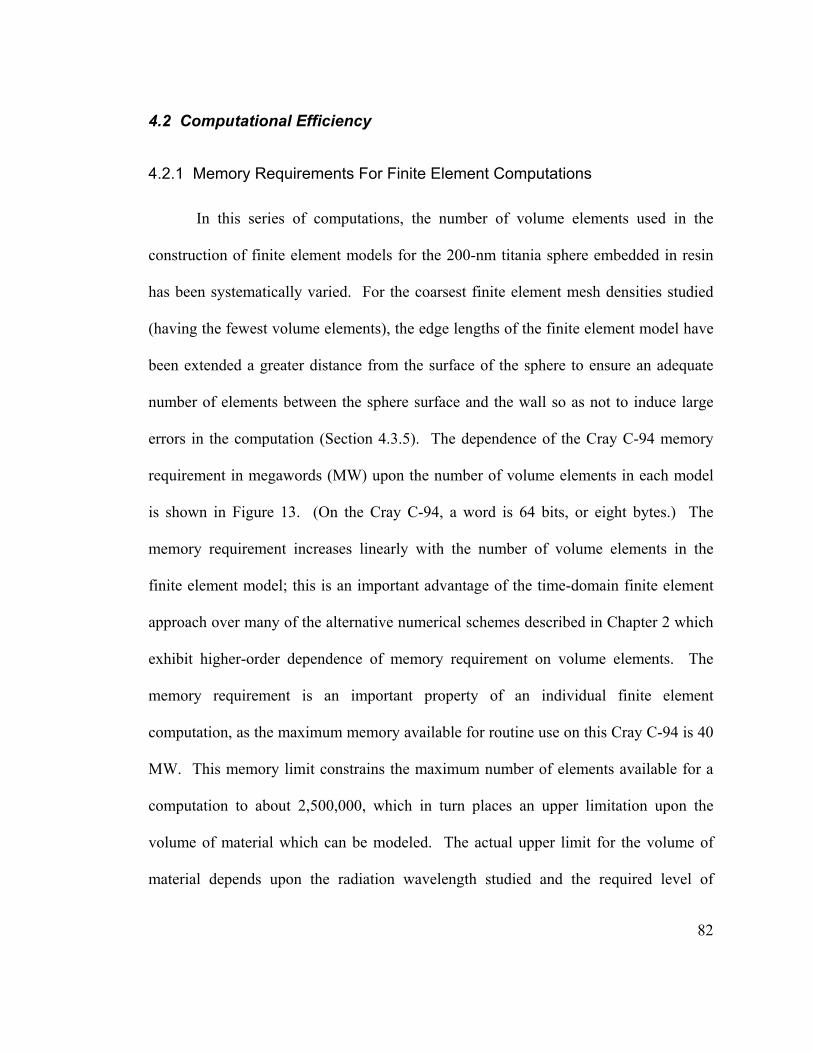
82

4.2 Computational Efficiency

4.2.1 Memory Requirements For Finite Element Computations

In this series of computations, the number of volume elements used in the

construction of finite element models for the 200-nm titania sphere embedded in resin

has been systematically varied. For the coarsest finite element mesh densities studied

(having the fewest volume elements), the edge lengths of the finite element model have

been extended a greater distance from the surface of the sphere to ensure an adequate

number of elements between the sphere surface and the wall so as not to induce large

errors in the computation (Section 4.3.5). The dependence of the Cray C-94 memory

requirement in megawords (MW) upon the number of volume elements in each model

is shown in Figure 13. (On the Cray C-94, a word is 64 bits, or eight bytes.) The

memory requirement increases linearly with the number of volume elements in the

finite element model; this is an important advantage of the time-domain finite element

approach over many of the alternative numerical schemes described in Chapter 2 which

exhibit higher-order dependence of memory requirement on volume elements. The

memory requirement is an important property of an individual finite element

computation, as the maximum memory available for routine use on this Cray C-94 is 40

MW. This memory limit constrains the maximum number of elements available for a

computation to about 2,500,000, which in turn places an upper limitation upon the

volume of material which can be modeled. The actual upper limit for the volume of

material depends upon the radiation wavelength studied and the required level of

83

accuracy of the computation, since it is the relationship between element size and

radiation wavelength that determines both the physical volume of the model and the

expected level of error in the computation.

Elements (x106)

0.0 0.3 0.6 0.9 1.2 1.5

Mem

ory

(MW

)

0

5

10

15

20

25

Figure 13. Dependence of Cray C-94 memory requirement upon the number of volume elements in the finite element model for the present series of EMFlex computations.

4.2.2 CPU Time Requirements For Finite Element Computations

The dependence of Cray C-94 CPU time upon the number of volume elements

in a finite element model for the series of computations described in Section 4.1.1 is

shown in Figure 14. As in the case of the memory requirement (Figure 13), CPU time

shows a linear dependence upon the number of volume elements in the finite element

model. This linear dependence is likewise an important advantage of the time-domain

finite element approach over many of the alternative numerical approaches described in

Section 2.3.3, such as the method of moments which exhibits a (N2) dependence of CPU

84

time upon the number of elements. It should be noted that the same number of wave

cycles (15) were allowed to propagate in the finite element model in each of the

computations in Figure 14. For fixed finite element model geometry, the Cray C-94

CPU time depends linearly upon the number of cycles allowed to propagate in a given

computation. CPU times of 45-60 minutes are typical of individual finite element

computations performed throughout this research. The vector nature of the Cray

architecture offers a factor of 3-10 speed-up over conventional scalar workstations with

the EMFlex code.

Elements (x106)

0.0 0.3 0.6 0.9 1.2 1.5

CPU

Tim

e (M

in.)

0

20

40

60

80

Figure 14. Dependence of Cray C-94 CPU time requirement upon the number of volume elements in the finite element model for the present series of EMFlex computations.

4.2.3 CPU Time Requirements For Far-Field Extrapolation

Once steady-state near-field quantities are computed using EMFlex in a finite

element model, these fields are extrapolated to far field using the Review software. As

85

described in Section 3.2.3, the surface of the far-field sphere onto which near-field

scattered intensities are extrapolated is divided into a number of surface elements

according to a spherical coordinate system. In the present series of computations, the

discretization in both angles theta and phi of the spherical coordinate system in the

extrapolation step has been systematically varied. The angular discretizations

investigated are 0.5, 1, 2, 3, 5, 10, and 15 degrees. The radius of the far-field sphere is

500 µm in all cases; the radius of the far-field sphere has no effect upon CPU time

required for the extrapolation. The CPU time required on the SGI Power Challenge

computer for a single far-field extrapolation is shown in Figure 15 as a function of the

angular discretization on the surface of the far-field sphere. This data indicates that the

required CPU time increases dramatically with increasing angular on the surface of the

far-field sphere. Over six hours of CPU time are required for 0.5-degree angular

discretization, while only about thirty minutes are required for 2-degree angular

discretization.

The data showing CPU time dependence upon angular discretization in Figure

15 has been plotted as a function of the number of surface elements on the far-field

sphere in Figure 16; the number of surface elements is proportional to the inverse

square of the angular discretization. The plot of CPU time as a function of the number

of surface elements shown in Figure 16 indicates that the dependence of CPU time upon

the number of surface elements on the far-field sphere is of higher order than linear.

The selection of angular discretization on the far-field surface affects CPU time

strongly, and this selection must therefore be made with consideration of the effect of

86

angular discretization upon accuracy of the far-field result. This accuracy issue is

described in Section 4.3.2.

Angular Discretization (Deg.)0 2 4 6 8 10 12 14 16

CPU

Tim

e (M

in.)

0

100

200

300

400

500

600

Figure 15. CPU time required for a single far-field extrapolation is shown in as a function of the angular discretization on the surface of the far-field sphere.

Surface Elements (x105)

0.0 0.3 0.6 0.9 1.2 1.5

CPU

Tim

e (M

in.)

0

100

200

300

400

500

600

Figure 16. CPU time required for a single far-field extrapolation is shown in as a function of the number of surface elements on the far-field sphere.

87

4.3 Computational Accuracy

4.3.1 Effects of Finite Element Mesh Density

The 200-nm titania sphere in polymeric resin is used here to determine the

influence of finite element mesh density upon the accuracy of the time-domain finite

element method. The size of the cubic volume elements in these computations is

expected to exert a strong influence upon the accuracy of the results, since the ability to

represent the geometries of curved particles such as spheres and to compute gradients in

electric field are both controlled by the size of the rectangular solid volume elements.

The most useful way to parameterize the finite element mesh density is to compare the

edge length of cubic volume elements composing a finite element model to the

wavelength of the electromagnetic radiation propagating in the model. Since the

effective wavelength of radiation propagating in a dielectric material is inversely

proportional to the refractive index of that material, it is the wavelength of a plane wave

traveling through the material with the highest refractive index nmax in the model that

effective should be considered. The minimum effective wavelength λmin in the model

is:

Equation 75 max

0min n

λλ =

where λ0 is the wavelength of the illuminating radiation in vacuum. In the present

series of computations, the highest index material in the model is the scattering sphere

with n = 2.74. The minimum wavelength of the 560-nm light in these computations is

88

therefore λmin = 560 nm/2.74 = 204 nm. The number of cubic volume elements per

minimum wavelength in the model is given by the unitless quantity ρ:

Equation 76 edgelminλ

ρ =

where ledge is the edge length of the cubic volume elements in the model. In the case of

the finite element models shown in Figure 10 and Figure 12, the values of ρ are 68 and

20, respectively.

The values of ρ investigated here are 10, 15, 20, 25, 30, 35, 45, 55, and 68. The

sphere diameter of 200 nm was used in each computation, and the edge length of the

finite element model were varied, when necessary, in order to maintain at least ten

elements between the sphere surface and the nearest model walls. In the extrapolation

to far field, the radius of the far-field sphere was 500 µm and the angular discretization

on the far-field sphere surface was 3 degrees in all cases. The scattering cross section

was computed for each case and compared with the exact result from Mie theory. The

resulting error is plotted in Figure 17 as a function of the finite element mesh density ρ.

As expected, the error increases with decreasing ρ, with an error less than 1% for ρ = 68

and an error greater than 8% for ρ = 10. Finite element mesh densities with ρ ≥ 20 are

used in all of the computations described in subsequent chapters of this dissertation, and

ρ ≥ 40 in most cases. These resolutions in the finite element mesh ensure that

maximum expected errors are limited to the values in Figure 17.

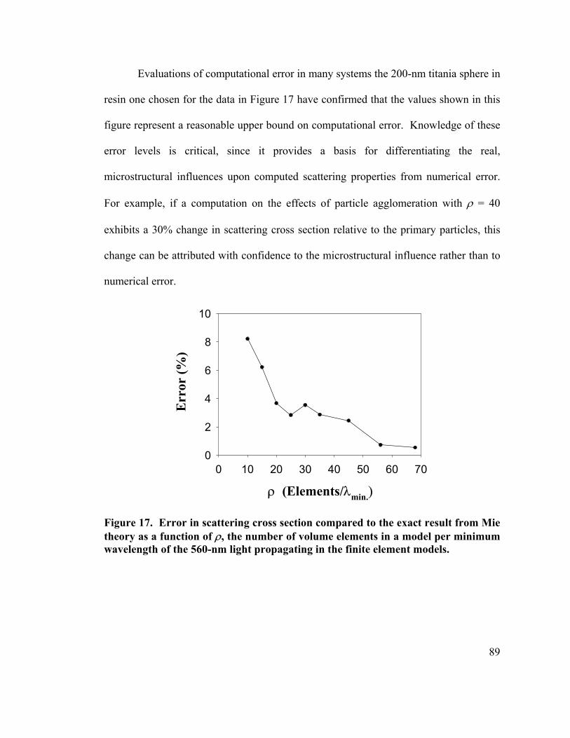
89

Evaluations of computational error in many systems the 200-nm titania sphere in

resin one chosen for the data in Figure 17 have confirmed that the values shown in this

figure represent a reasonable upper bound on computational error. Knowledge of these

error levels is critical, since it provides a basis for differentiating the real,

microstructural influences upon computed scattering properties from numerical error.

For example, if a computation on the effects of particle agglomeration with ρ = 40

exhibits a 30% change in scattering cross section relative to the primary particles, this

change can be attributed with confidence to the microstructural influence rather than to

numerical error.

ρ (Elements/λmin.)

0 10 20 30 40 50 60 70

Err

or (%

)

0

2

4

6

8

10

Figure 17. Error in scattering cross section compared to the exact result from Mie theory as a function of ρ, the number of volume elements in a model per minimum wavelength of the 560-nm light propagating in the finite element models.

90

4.3.2 Effects of Mesh Density on Surface of Far Field Sphere

In Section 4.2.3, the effects of angular discretization on the surface of the far-

field sphere upon the CPU time required for extrapolation of fields from near to far field

were described. Here, the errors in scattering cross section for that same series of

computations are compared to the exact result from Mie theory. These results are

plotted in Figure 18 as a function of angular discretization on the far-field sphere

surface. As expected, computational error increases with decreasing angular resolution.

The error increases non-linearly with angular discretization, with an error of ~0.7% for

all values less than or equal to 3 degrees. For values greater than 3 degrees, error

increases rapidly with increasing angular discretization. As shown in Figure 15, the

CPU time required for extrapolation decreases very rapidly with increasing angular

discretization on the surface of the far-field sphere; there is therefore a trade-off

between increased accuracy and increased CPU time in extrapolation of near-field

results to far field. This trade-off is well-balanced for the angular discretization 2-3

degrees, which is the range of values typically used in this research. Investigation of

error as a function of the illumination angle have confirmed that these values yield good

accuracy while requiring reasonable CPU times for the computation.

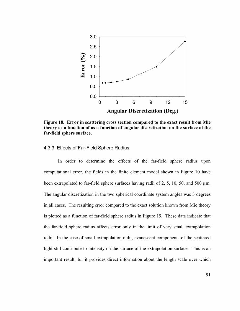
91

Angular Discretization (Deg.)0 3 6 9 12 15

Err

or (%

)

0.0

0.5

1.0

1.5

2.0

2.5

3.0

Figure 18. Error in scattering cross section compared to the exact result from Mie theory as a function of as a function of angular discretization on the surface of the far-field sphere surface.

4.3.3 Effects of Far-Field Sphere Radius

In order to determine the effects of the far-field sphere radius upon

computational error, the fields in the finite element model shown in Figure 10 have

been extrapolated to far-field sphere surfaces having radii of 2, 5, 10, 50, and 500 µm.

The angular discretization in the two spherical coordinate system angles was 3 degrees

in all cases. The resulting error compared to the exact solution known from Mie theory

is plotted as a function of far-field sphere radius in Figure 19. These data indicate that

the far-field sphere radius affects error only in the limit of very small extrapolation

radii. In the case of small extrapolation radii, evanescent components of the scattered

light still contribute to intensity on the surface of the extrapolation surface. This is an

important result, for it provides direct information about the length scale over which

92

near-field optical interactions in this system are important. For radii greater than or

equal to 10 µm, there is no dependence of error upon the extrapolation radius. In all

cases, the CPU time required for extrapolation was independent of the extrapolation

radius. Based upon the results shown in Figure 19, a far-field sphere radius of 500 µm

is used in all subsequent far-field extrapolations in this research.

Log10[Far-Field Radius (µm)]0 1 2 3

Err

or (%

)

0.5

0.6

0.7

0.8

0.9

1.0

Figure 19. Error in scattering cross section compared to the exact result from Mie theory as a function of as a function of far-field sphere radius.

4.3.4 Effects of Kirchoff Box Placement in the Model

Using the model shown in Figure 10, the position of the Kirchoff box

surrounding the scattering sphere in this model has been systematically varied to

determine its effects upon computational error. The Kirchoff box is the mathematical

surface on which equivalent electric and magnetic currents are computed for subsequent

extrapolation of near-field results to far field (Section 3.2.1). The Kirchoff box surface

93

must be sufficiently displaced from the particle surface (where electric field gradients

are potentially greatest) and from the model walls (where electric field values may be

spuriously influenced by the boundary conditions). The usual placement of the

Kirchoff box is just inside the walls of the model but with sufficient space between it

and the wall to prevent boundary condition effects from introducing errors into the

extrapolation.

Using the model shown in Figure 10, the Kirchoff box was placed precisely

half-way between each wall of the model and the surface of the sphere. The error in the

scattering cross section for this calculation (compared to the exact solution known from

Mie theory) was 0.76%. In subsequent calculations, the six sides of the Kirchoff box

were progressively moved closer to the surface of the spherical particle. With just two

elements separating the Kirchoff box from the sphere surface on all six sides, the error

in scattering cross section was 0.79%, indicating no deviation from the previously cited

result. With the Kirchoff box just one element away from the sphere surface, however,

the error in scattering cross section increased to 4.3%, suggesting that the presence of

strong electric field gradients immediately at the sphere surface caused significant error

in the extrapolation operation. The Kirchoff box was then moved progressively closer

to the walls of the model from the half-way point between the sphere and the model

walls. With the Kirchoff box positioned two elements away from the model walls on all

six sides, the error in scattering cross section was 0.75%, in good agreement with case

where the Kirchoff box was farther removed from the model wall. With the Kirchoff

box just one element away from the model wall, however, the error jumped to 186%, a

94

result of errors in electric field vectors and gradients produced by the boundary

conditions at the model walls.

The results described in this section indicate that the positioning of the Kirchoff

box can affect the accuracy of these finite element calculations. No significant

problems are anticipated, however, provided that the sides of the Kirchoff box are

several elements removed from both the surfaces of the scattering particle and the

model walls.

4.3.5 Effects of Particle Position Relative to Model Walls

Illumination boundary conditions (Section 3.2.1), which are intended to absorb

only scattered radiation, are used at each of the six model walls of finite element models

throughout this research. Since scattered light can be spuriously reflected back into the

model at the walls due to the imperfection of the boundary condition, increased error

could be expected as the intensity of scattered radiation encountering the walls

increased. To investigate these effects, the 200-nm titania sphere shown in Figure 10

was displaced from the top edge of the model to the bottom edge over a series of four

computations. Figure 20 shows the steady-state scattered electric field intensities on

cross-sectional slices through the centers of these four models. The 560-nm light

propagates in the +x direction in each case. It is evident in Figure 20 that the forward

scattered light interacts more strongly with the bottom wall of the model as the sphere

moves closer to it, with the extreme case appearing in the bottom right panel of the

95

figure. The distances between the bottom surface of the sphere and the bottom of the

model in these four models are listed in Table 1.

Table 1 summarizes the results of extrapolating the near-field scattering results

shown in Figure 20 to far field. The results of this extrapolation have been compared to

the exact scattering cross section known from Mie theory; the errors associated with

those computations are presented in Table 1. Interestingly, the error in scattering cross

section decreases systematically as the scattering sphere is moved closer to the bottom

wall of the model (or, alternatively, away from the top of the model). This observation

was surprising; it was expected that increased interaction of forward-scattered light with

the bottom wall of the model would cause increased error. The results of Table 1

provide no evidence that such a problem arose in these computations. An important

result the data in Table 1 is that there is no evidence that the interaction between the

forward scattered light and the model wall has caused the computation to fall into

severe error. This result is encouraging, since it suggests that it is not necessary to

provide large volumes of surrounding medium in the forward-scattering direction,

allowing the implementation of models containing fewer volume elements and therefore

requiring shorter CPU times for computation. It is possible that the increased error

associated with longer distances between the sphere and the bottom wall of the model is

a result of resonance between forward-scattered light and the bottom model wall. These

effects could also occur in the back-scattered direction (i.e., between the top of the

sphere and the top model wall in Figure 20), but they would be substantially weaker

since significantly less light is back-scattered than forward-scattered.

96

Figure 20. Cross-sectional slices through the centers of four finite element models in which the spacing between the 200-nm sphere and the bottom wall of the model has been systematically varied. Scattered light intensity is shown in each case.

97

Table 1. Error in scattering cross section as a function of separation distance between the bottom of the sphere and the

bottom wall of the model. The corresponding models are shown in Figure 20.

Sphere-Bottom Wall Distance (nm) Error (%)

185 1.9

150 0.74

85 0.21

20 0.02

4.3.6 Effects of Model Dimensions Compared to Light Wavelength

In addition to Kirchoff box and model wall placement, the edge length of a finite

element model compared to the radiation wavelength can have significant impact upon

computational error. Figure 21 shows a finite element model of a 40-nm titania sphere

with refractive index n = 2.74 embedded in the polymeric resin with refractive index n =

1.51. As in all previous computations in this chapter, the wavelength of the incident

light is 560 nm. This represents a non-resonant case in the Rayleigh scattering regime.

Referring to the plot of the scattering coefficient S as a function of sphere diameter

shown in Figure 8, the 40-nm sphere diameter is very weakly scattering compared to the

200-nm sphere diameter. The edge length of the model shown in Figure 21 is 400 nm,

and light propagates in the +x direction. The two panels of Figure 21 showing near-

field scattered intensity indicate that the particle scatters light nearly isotropically rather

than in the forward direction, which is expected in the Rayleigh regime. To investigate

98

the effects of model size upon accuracy of these finite element computations, the edge

length of the cubic model in this series of computations was systematically varied

between 100 and 400 nm, without changing the edge length of the cubic volume

elements composing the model. The scattering sphere was located at the center of the

model in all cases.

The columns of Table 2 show the edge length of the model, the optical length of

the model, and the percent error in scattering cross section versus the known result from

Mie theory for each case. The optical length of the model, which is defined here as the

number of wavelengths of light which would exist along the linear path from the top to

the bottom of the model which passes through the center of the sphere. Since the

refractive indices of the sphere and the surrounding medium are both greater than unity,

the wavelength of radiation propagating in these materials is compressed. The optical

length is the sum of the individual propagation distances through the different media

present in the model multiplied by their respective refractive indices, divided by the free

wavelength of the incident light:

Equation 77 ( ) 02211. /... λ++= nlnllopt

For example, in the case of the finite element model in Figure 21 with 400-nm edge

length, a line passing from the top of the model to the bottom and passing through the

center of the 40-nm sphere encounters 40 nm of material with n = 2.74 (the sphere) and

360 nm with n = 1.51 (the surrounding medium). The optical length is therefore

computed as:

99

Equation 78 ( )[ ] 16.1560/514.136074.240. =⋅+⋅= nmnmnmlopt .

As Table 2 indicates, the error in scattering cross section is strongly dependent

upon the edge length of the model. For models smaller than 400 nm on edge, error

increases abruptly from roughly 1% to the range 17-41%. These effects are attributed

to the size of the model relative to the light wavelength. In the case of models which

are so small compared to the light wavelength that the optical length is less than unity,

the problem of not developing a steady-state, propagating wave in the model arises.

Instead of at least one full wavelength of light propagating through the model, electric

field amplitudes in the model can fluctuate unstably in response to the fluctuating

electric field of the incident radiation, to which most of the model is at once subject.

The same analysis shown in Table 2 has also been applied to the problem of the

more resonant 200-nm sphere described in the preceding section. In this series of

experiments, the 200-nm sphere with n = 2.74 has been placed at the center of a cubic

model with a surrounding medium with n = 1.51 and the edge length of the model

systematically decreased until it was in close proximity to the surface of the particle.

The results of this series of experiments, shown in Table 3, support the idea that models

must be sufficiently large to ensure that the optical length of the model is greater than

unity in order to avoid large errors in scattering cross section in these finite element

computations. Comparing results from Table 2 and Table 3, it appears that an optical

length of 1.2 is sufficient to ensure minimal computational errors for the materials

employed in these two series of computations.

100

Figure 21. Finite element model of a 40-nm sphere with n = 2.74 embedded in a polymeric resin with n = 1.51. The 560-nm illuminating light propagates in the +x direction and is polarized in the z direction.

101

Table 2. Error in scattering cross section of finite element calculations in which the model edge length was systematically

varied. All calculations are for the case of a 40-nm sphere at the center of a cubic model.

Model Edge Length (nm) Optical Length % Error

100 0.4 41

200 0.6 26

300 0.9 17

350 1.0 30

400 1.2 0.9

Table 3. Error in scattering cross section of finite element calculations in which the model edge length was systematically

varied. All calculations are for the case of a 200-nm sphere at the center of a cubic model.

Model Edge Length (nm) Optical Length % Error

234 1.07 4.7

254 1.12 1.9

272 1.17 0.94

300 1.25 0.97

102

4.3.7 Effects of Strong Resonance: High-Index Spheres in Vacuum

As the mismatch between the refractive index of a sphere and the medium in

which it is embedded is increased, the maximum scattering efficiency which is

attainable increases. This is illustrated in the following example calculated using Mie

theory. Figure 8 shows a plot of scattering coefficient S (µm−1) versus diameter for the

case of a sphere with refractive index n = 2.74 embedded in a medium with n = 1.51.

The maximum value observed, representing the most resonant condition, is S ≈ 26 µm−1

for the sphere diameter 200 nm. Figure 22, in comparison, shows a plot of S versus

diameter for the case of a sphere with n = 3.0 embedded in a medium with n = 1.0 (e.g.,

air or vacuum). The maximum value observed in this case is S ≈ 68 µm−1 for the sphere

diameter 177 nm, a substantially greater value than the previous case considered. This

higher value implies much greater scattered intensities and electric fields gradients at

near field. These make this highly resonant system more susceptible to errors

associated with the mesh density and its ability to describe sharp gradients accurately.

To quantify the computational error of the time-domain finite element approach

in highly resonant cases, the three sphere diameters marked with “x” in Figure 22 have

been investigated. The point corresponding to the first resonant peak in this figure

(diameter 0.177 µm) is the most strongly resonant condition and therefore the most

difficult to model accurately using the finite element approach. The other two points,

corresponding to sphere diameters 0.16 and 0.22 µm, are not as strongly resonant and

lower numerical errors are expected in these cases.

103

The results of these calculations are summarized in Table 4. The errors

associated with the calculations for the less resonant cases (sphere diameters 0.16 and

0.22 µm) are both less than 1%, indicating very close agreement with the known

solutions from Mie theory. The error associated with the strongly resonant case (sphere

diameter 0.177 µm), on the other hand, is 6.4%, deviating substantially from the exact

solution. This series of calculations demonstrates that error in the time-domain finite

element approach depends upon the degree of resonance in a specific calculation as well

as the factors identified above. It should be noted that the extreme contrast ratio of m =

3.0 between the sphere and the surrounding medium in the case studied here exceeds

any which is encountered in practice; there are no known, non-lossy dielectric materials

with refractive index as high as 3.0. The calculations described in this section are

therefore non-physical but nevertheless highlight the effects of resonance upon

computational accuracy of the finite element method.

104

0

10

20

30

40

50

60

70

0 .05 .1 .15 .2 .25 .3 .35

S

Sphere Diameter (Microns)

( m

)

µ−1

x

x

x

Figure 22. The scattering coefficient S (µm−1) as a function of sphere diameter for the case of a sphere with n = 3.0 in a medium with n = 1.0. This represents a more resonant system than can be achieved in practice, since no known, non-lossy material exhibits such a high refractive index in the visible spectrum.

Table 4. Error in scattering cross section as a function of sphere diameter for the three cases indicated on the plot

in Figure 22.

Sphere Diameter (nm) Error (%)

160 0.64

177 6.4

220 0.85

105

4.4 Guidelines For Building Robust Finite Element Models

The observations of the present chapter may be used to formulate a set of simple

guidelines for the construction of robust finite element models for the EMFlex software.

These guidelines are designed to minimize the error of the finite element. They are:

1. The optical length (Equation 77)of the finite element model edges should be

at least 1.2 wavelengths.

2. The finite element mesh should be as fine as memory limitations allow.

3. The scattering microstructure should be positioned at the center of the

model.

4. The scattering microstructure should be at least eight elements from any

model wall.

5. The Kirchoff surface should be placed at least three elements from any

model wall and the scattering microstructure.

6. The surface of the far-field extrapolation surface should be placed a very

large optical distance from the finite element model.

7. The angular mesh on the surface of the far-field extrapolation surface should

be as fine as possible to ensure minimal error; CPU time restrictions are the

limitation here.

106

Chapter 5. A Potpourri of Pigment Particles

In this chapter, the light scattering properties of three different white pigment

systems are determined using computational modeling. In Section 5.1, Mie theory

computations are performed for the case of core-shell composite pigment architectures

for the case of coated spheres. In this study, the average index approximation for rutile

titania is used; titania is modeled as an optically isotropic material. This assumption is

justified, since the most dramatic changes in scattering behavior arise from the presence

of the second material in the coated particle. In Section 5.2, the time-domain finite

element approach is used to determine the light scattering behavior of optically

anisotropic spheres of rutile titania. These results are compared to the average index

and weighted sum approximations to determine their ability to describe the scattering

efficiency of rutile titania. Finally, in Section 5.3, the light scattering properties of a

morphological rutile titania particle are computed using the time-domain finite element

method. These results are compared to the scattering performance of the equivalent-

volume sphere under both the average index and weighted sum approximations. In

addition, the scattering data are used to calculate equivalent spherical diameters in order

to highlight the difficulties in particle size analysis which can arise in modeling

complex particle shapes as simple spheres.

107

5.1 Core-Shell Pigment Particles

5.1.1 Introduction

One of the largest market segments for titania white pigment is the paper

industry. Since titania is more expensive than pulp and the other mineral pigments

which are used in paper formulations, such as kaolin clay and calcium carbonate,

formulators of paper systems attempt to use titania as efficiently as possible. In paper

applications, it is normally most cost-effective to optimize the content of the non-titania

components and then add titania as required to achieve target opacity. Formulation

strategies for optimization of both paper furnish and coating formulations have been

proposed by Houle1 and Kwoka.2,3,4

Recently, it has been proposed that the scattering efficiency of white pigment

can be improved by coating spherical silica particles with a titania shell.22,23,24 The

lower titania content of such particles suggests that they could potentially provide better

value versus pure titania pigments. To address this issue, the light scattering properties

of model core-shell pigments have been determined using a computational approach.

Results are presented below for the general case of a titania shell over cores with

refractive index varying from 1.0 (hollow titania spheres) up to 2.74 (solid titania

spheres). This is followed by a comparison of the scattering performance of titania-

coated silica versus pure titanium dioxide.

108

5.1.2 Scattering Properties of Titania-Coated Core-Shell Pigments

A schematic diagram of the configuration for the titania-coated core-shell

particles is shown in Figure 23. All critical parameters are indicated. The core is a

sphere of diameter DC. The titanium dioxide coating forms a shell with outside

diameter DT. The reported calculations include particles with shell diameters up to 1

µm and consider the full range of 100% titania (i.e., DC = 0) to 100% core material

(i.e., DC = DT). In the case of a silica core, for example, it is not practical to deposit

more than 40 weight percent titania on the core. Since the volume percent titania is

related to the cube of DC/DT and since titania is more dense than silica, this composition

corresponds to a thin shell around the silica core, with a shell diameter only 10% larger

than the core. For clarity, the schematic diagram in Figure 23 illustrates a particle with

a shell diameter about 20% larger than the core diameter. This represents an

impractical case with a titania content of 64 wt %. For practical cases, the thickness of

the titania layer would be much thinner than illustrated.

109

Core

DC

nC : Air 1.0 SiO2 1.46

DT

Core Diameter

TiO2 Shell Diameter

TiO2 Shell

nT = 2.74

Surrounding MediumCellulose or

Paper Coating{ }nm = 1.45

Figure 23. Schematic representation of titania coated on a core particle of lower refractive index.

The other key parameters in Figure 23 are the refractive indices of the

component materials. The value of 2.74 for titania is the average refractive index at the

center of the visible spectrum. The refractive index of the core is an independent

variable. A core refractive index of 1.0 (air) represents a hollow titania shell, while a

core index of 1.46 represents titania-coated silica. A core with refractive index equal to

that of rutile titania represents a solid rutile particle. The refractive index for the

surrounding medium in a paper system is more difficult to assign. The value of 1.45

used in these calculations is the average refractive index of a representative paper

coating composed of a mixture of clays and calcium carbonate (refractive index 1.6),

starch or latex binders (refractive index 1.5), and air voids (refractive index 1.0).

Uncoated papers are composed of cellulose fiber (refractive index 1.45), clays, calcium

110

carbonate, and air voids. A refractive index lower than 1.45 should be used to represent

the surroundings for titania in filled sheet applications.

5.1.2.1 Refractive index of medium at 1.45

A plot of the angle-weighted scattering coefficient σ for the general case of

rutile titania-coated cores in a paper coating or cellulose matrix is shown in Figure 24.

The results were calculated for the light wavelength 560 nm, the center of the visible

spectrum. This is the wavelength where the human eye is most sensitive and close to

the center of the wavelength bands used for measurement of paper opacity. Absolute

values of scattering coefficients are dependent on wavelength, but results calculated at

560 nm provide a sound representation of the light scattering properties that affect

opacity.

For the particles in Figure 24, the ratio of the core diameter to total diameter,

DC/DT, is fixed at 0.9. The three-dimensional plot shows the scattering efficiency for

particles with outer diameter, DT, from 0.0 to 1 µm. Each contour line represents the

dependence of σ on diameter for a given core refractive index. The refractive index of

the core material is incremented by 0.035 with each contour line and ranges from 1.0

(air) to 2.74 (rutile). The global maximum of this plot, indicating the optimally

scattering particle structure, corresponds to a solid rutile particle (core and shell

refractive index both equal to 2.74) with of diameter 0.2 µm.

In the case of titania-coated silica, the core index is 1.46. The data in Figure 25

are plotted as a function of the diameters of the silica core and the titania shell

111

diameters, both of which vary in the range 0.0−1.0 µm. Each contour line represents a

0.002 µm increment of outer shell diameter. As in Figure 24, the global maximum

corresponds to a solid rutile sphere (i.e., silica core diameter equal to zero). Variation

of the core and shell diameters results in the undulating series of local minima and

maxima in Figure 25. The greatest local maximum corresponding to a sphere having

substantial silica content occurs at a titania shell diameter of about 0.35 µm, with a

silica core diameter of about 0.2 µm. The σ value associated with this coated silica

particle is only about 64% that of the optimized solid rutile sphere.

112

11.5

22.5

3

0

2

4

6

8

10

12

0 .2 .4 .6 .8 1

σ

Sphere Diameter (Microns)

Core I

ndex

( m

)

µ-1

Figure 24. Scattering coefficient σ (µm−1) versus coated particle diameter and refractive index of the core material for titania-coated particles with coating thickness equal to 10% of the particle radius.

.2.4

.6.8

1

0

5

10

0 .2 .4 .6 .8 1 A r b it r a r y Y / A r b it r a r y X

( m

)

Silica Core Diameter (Microns)

TiO S

hell D

iamete

r (M

icron

s)

2

µ-1

σ

Figure 25. Scattering coefficient σ (µm−1) versus silica core diameter and titania shell diameter for a coated particle. The global maximum of this plot corresponds to a solid titania sphere of 0.2 µm diameter.

113

For greater clarity, five contours have been extracted from the three-dimensional

plot in Figure 25 and shown in the two-dimensional plot of Figure 26. This figure

shows σ as a function of silica core diameter for spheres having five different titania

shell diameters. The sphere with titania shell diameter 0.20 µm is that which exhibits

the highest σ value associated with solid titania (silica core diameter equal to zero).

There is an obvious decrease in σ with increasing silica core diameter. Many of the

titania-coated silica particles nearly match the scattering efficiency of the pure titania

particles with the same outside diameter, but each is deficient relative to pure titania at

its optimum diameter. For example, in the case of particles with titania shell diameter

0.5 µm, the scattering coefficient is nearly constant as the silica core is increased from 0

to 0.4 µm. The scattering coefficient of this set of particles is 70% below that of the

optimized solid titania particle. A sphere with titania shell diameter 0.35 µm is the

particle which exhibits the highest σ value among those spheres containing a substantial

amount of silica (silica core diameter 0.2 µm). This core-shell particle has DC/DT =

0.2/0.35 = 0.57 and a titania content of 89 weight percent, which means that the titania

coating is impractically thick from a synthesis standpoint. All other silica-containing

particles exhibit even lower σ values than those having titania shell diameters of 0.35

and 0.5 µm.

As noted previously, physically realizable core-shell architectures are limited to

those with a titania shell thickness that is less than or equal to 10% of the outer particle

diameter (DC/DT = 0.9) This limiting case has been plotted in Figure 27, which shows σ

114

as a function of sphere diameter both for solid titania and for coated particles with

DC/DT = 0.9. The results for the two structures are strikingly different; the maximum σ

value achieved by a solid titania sphere is 10.5 µm−1, while the maximum value

achieved by the silica-coated particle is only about 1.7 µm−1. The two curves are

approximately equal for particle diameters greater than ~0.7 µm. The resonant peaks

observed in Figure 27 for the pure rutile particles are an artifact the high spatial

symmetry of a sphere. In practice, these surface wave resonances are not

experimentally observed even for particles with narrow size distributions.5

0

2

4

6

8

10

0 .2 .4 .6 .8 1 r b it r a r y Y / A r b it r a r y X

( m

)

Silica Core Diameter (Microns)

0.35 um

Titania shell diameter 0.2 um

0.5 um0.75 um

1.0 um

µ−1

σ

Figure 26. Scattering coefficient σ for five coated particles with different outside diameters.

115

0

2

4

6

8

10

0 .2 .4 .6 .8 1 i t r a r y Y / A r b it r a r y X

( m

)

Particle Diameter (Microns)

µ-1

Pure Rutile

10% Rutile on Silicaσ

Figure 27. Scattering coefficient σ versus particle diameter for a solid titania sphere and a titania-coated silica particle with coating thickness equal to 10% of the particle radius.

The Mie theory computations presented here describe the light scattering

properties of an isolated spherical particle and cannot be applied to systems in which the

crowding effect is important. However, crowding can be viewed as agglomeration of

individual particles into clusters. If the scattering properties of these clusters could be

reasonably approximately by computing the scattering properties of equivalent-volume

spheres, the data in Figure 27 at higher diameters suggest that optimized rutile particles

will show more loss due to crowding than particles of titania-coated silica. This effect

will not apply for most paper applications where titania concentrations are below ~15%

by volume.

The incentive for depositing titania coatings on a low density and inexpensive

core material like silica is to attempt to increase the light scattering efficiency per pound

of pigment or to reduce the price of the pigment. The scattering coefficients in Figure

116

24–Figure 27 can be divided by the density of the coated particle, thereby expressing σ

on a weight basis (m2/g). Using specific gravities of 2.2 g/ml for silica and 4.26 g/ml

for rutile titania, the data in Figure 25 were normalized by dividing by the density of the

particle; these results are shown in Figure 28. While this normalization scheme has the

effect of slightly increasing the effective σ values of those particles containing silica,

the global maximum in Figure 28 nevertheless corresponds to a solid titania sphere,

with no silica present, as in Figure 24–Figure 27.

It is also of interest to normalize the light scattering data in Figure 25 by

dividing the σ values by the weight fraction of titania present in the particle. This

normalization scheme reveals the relative scattering efficiency for the limiting case

where the value of the titania-coated silica pigment is assessed only by its titania

content. The results of this normalization scheme are shown in Figure 29. This data

does not include the diverging σ values which occur for those cases where the titania

coating thickness approaches zero. Even with this normalization scheme, the global

maximum in Figure 29 corresponds to a solid titania sphere, with no silica present.

117

.2.4

.6.8

1

0

1

2

3

0 .2 .4 .6 .8 1 r b it r a r y Y / A r b it r a r y XSilica Core Diameter (Microns)

TiO S

hell D

iamete

r (M

icron

s)

2

σ(D

ensit

y-N

orm

aliz

ed)

Figure 28. Scattering coefficient σ divided by the density of the coated particle. The global maximum of this plot corresponds to a solid titania sphere with no silica present.

.2.4

.6.8

1

0

5

10

0 .2 .4 .6 .8 1 A r b it r a r y Y / A r b it r a r y X

(Nor

mal

ized

by

TiO

Wt.

Frac

.)

Silica Core Diameter (Microns)

TiO S

hell D

iamete

r (M

icron

s)

2

2

σ

Figure 29. Scattering coefficient σ divided by the weight fraction of titania present in each coated particle. The global maximum of this plot corresponds to a solid titania sphere with no silica present.

118

Finally, the light scattering performance of the silica-titania core-shell pigments

can be compared to a heterogeneous mixture of the two pure pigments to determine

whether any synergy results for the coated particles. For the titania-coated silica

particles in Figure 27, DC/DT is 0.9 which corresponds to 27.1 volume percent titania.

The highest σ value of 1.70 µm−1 occurs for the titania-coated silica at the diameter

0.687 µm. For pure rutile, the optimal σ value of 10.574 µm−1 occurs at the diameter

0.20 µm. For pure silica, the optimal σ value for pure silica is very low because the

refractive index is close to that of the medium; the optimum occurs at the diameter 0.20

µm but is only σ = 0.0005 µm−1. For a heterogeneous mixture of optimized rutile and

silica spheres, the scattering coefficient σmix is calculated using volume fraction, φ of

each component:

Equation 79 2222 SiOSiOTiOTiOmix σφσφσ +=

For the core-shell particle containing 27.1 volume % titania, φTiO2 is 0.271 and φSiO2 is

0.729. Therefore, σmix for the mixture of titania and silica spheres computed from

Equation 79 is 2.866 µm−1, which is 1.7 times greater than the scattering coefficient for

the same volumes of titania and silica in the optimized core-shell structure. Similar

evaluations of other combinations of DC and DT for silica and titania also reveal no

evidence of synergy in the scattering properties of the core-shell structures.

5.1.2.2 Refractive index of medium at 1.0 (air)

White pigment particles in filled paper applications are not surrounded only by

cellulose (refractive index 1.45) but instead by both cellulose and air. To address this

119

point, these calculations have been modified by changing the index of refraction of the

surrounding medium from 1.45 to 1.0, that of air. With a surrounding matrix of air, the

difference in σ between the optimized titania sphere and titania-coated silica spheres is

even more pronounced. Figure 30 shows a plot of σ versus silica core diameter for the

five core-shell particles shown in Figure 26. The σ value for a solid titania sphere with

diameter 0.20 µm in Figure 30 is σ ≈ 28 µm−1, while the value for a titania-coated silica

sphere with outer diameter 0.35 µm and silica core diameter 0.3 µm is σ ≈ 10 µm−1.

This difference is much more pronounced than the values observed in Figure 26. Since

pure rutile particles outperform titania-coated silica particles in both a cellulose matrix

and an air matrix, it can be concluded that rutile particles are also more efficient in

porous paper substrates, in which the medium surrounding the particles is a mixture of

cellulose and air.

120

0

10

20

30

0 .2 .4 .6 .8 1 i t r a r y Y / A r b it r a r y X

( m

)

Silica Core Diameter (Microns)

0.35 um

Titania shell diameter 0.2 um

0.5 um

0.75 um1.0 um

µ−1

σ

Figure 30. Scattering coefficient σ for the five particles shown in Figure 26, with the cellulose surrounding medium replaced by air (refractive index 1.0 instead of 1.45).

5.2 Anisotropic Spheres of Rutile Titania

5.2.1 Introduction

Attempts to use Mie theory to predict the light scattering properties of a rutile

titania particle require approximation to address the optical anisotropy of the crystal.

Rutile titania is uniaxial, exhibiting its ordinary refractive index for light polarized

parallel to either the a or b axis of the crystal and its extraordinary refractive index for

light polarized parallel to the c axis. In this section, the light scattering properties of

optically anisotropic spheres of rutile titania have been computed directly for the first

time using the time-domain finite element approach.

121

As described in Section 2.2.1, two methods for approximating rutile as an

isotropic material have been proposed in the literature. One approach has been to

compute the mean of the refractive indices along the three crystal axes at the light

wavelength of interest18 and subsequently apply Mie theory to compute far-field

scattering parameters. This is the average index approximation. For the light

wavelength 560 nm, the average refractive index of rutile titania is 2.74. In these

computations, the refractive index of the surrounding medium is 1.51, representing a

typical paint resin. The results of Mie theory computations for the scattering coefficient

S using the average index approximation are shown in Figure 31 as a plot of S versus

sphere diameter. The greatest S values occur for sphere diameters in the range 0.18-

0.30 µm, with a maximum value of S = 27.74 µm−1 for the diameter 0.272 µm.

Likewise, the results of Mie theory computations for the angle-weighted scattering

coefficient σ using the average index approximation are shown in Figure 32. The

maximum value of the angle-weighted scattering coefficient σ = 12.17 µm−1 occurs for

the sphere diameter 0.20 µm.

A second method for approximating the scattering behavior of rutile titania

using isotropic materials has been to compute separately far-field scattering parameters

for an isotropic sphere having the ordinary and extraordinary refractive indices of rutile

titania, and subsequently compute the weighted sum of these separate far-field

results.17,18 The weighted sum consists of two-thirds the result for the ordinary

refractive index plus one-third the result for the extraordinary refractive index. This is

the weighted sum approximation. The results of Mie theory computations for the

122

scattering coefficient S using the weighted sum approximation are shown in Figure 33

with S plotted as a function of sphere diameter. This result exhibits less pronounced

resonant peaks in S than the analogous plot generated using the average index

approximation shown in Figure 31. This is expected, since the resonant peaks in the

two individual curves used to form the weighted sum are systematically offset from one

another. The maximum S values for the weighted sum approximation occur in the

range 0.18−0.3 µm, as with the average index approximation. The maximum value S =

25.08 µm−1 occurs for the diameter 0.270 µm, about 10% lower than the maximum

value S = 27.74 µm−1 observed in the case of the average index approximation. The

angle-weighted scattering coefficient σ using the weighted sum approximation is shown

in Figure 34. This curve is in close agreement with that computed using the average

index approximation, shown in Figure 32. In the case of the weighted sum

approximation, the maximum value of the angle-weighted scattering coefficient σ =

11.71 µm−1 occurs for the sphere diameter 0.204 µm, about 4% lower than the

maximum value of the angle-weighted scattering coefficient σ=12.17 µm−1 observed in

the case of the average index approximation.

The average index and weighted sum approximation results shown in Figure

31−Figure 34 will be used as bases for comparison with results for anisotropic spheres

of rutile titania computed using the time-domain finite element method. Results

obtained using the finite element method contain the effects of the optical activity of the

uniaxial crystal, unlike the results of the average index or weighted sum approximations

based upon scattering by isotropic spheres.

123

0

5

10

15

20

25

30

0 .2 .4 .6 .8 1

S

Sphere Diameter (Microns)

( m

)

µ−

1

Figure 31. Scattering coefficient S versus sphere diameter for an optically isotropic sphere from Mie theory, using the average index approximation.

0

2

4

6

8

10

12

0 .2 .4 .6 .8 1

σ

Sphere Diameter (Microns)

( m

)

µ−

1

Figure 32. Angle-weighted scattering coefficient σ versus sphere diameter for an optically isotropic sphere from Mie theory, using the average index approximation.

124

0

5

10

15

20

25

30

0 .2 .4 .6 .8 1

S

Sphere Diameter (Microns)

( m

)

µ−

1

Figure 33. Scattering coefficient S versus sphere diameter for an optically isotropic sphere from Mie theory, using the weighted sum approximation.

0

2

4

6

8

10

12

0 .2 .4 .6 .8 1

σ

Sphere Diameter (Microns)

( m

)

µ−

1

Figure 34. Angle-weighted scattering coefficient σ versus sphere diameter for an optically isotropic sphere from Mie theory, using the weighted sum approximation.

125

5.2.2 Scattering By Anisotropic Spheres of Rutile Titania

The light scattering properties of anisotropic, high-index spheres assigned the

optical constants of rutile titania with diameters in the range 50−350 nm have been

computed using the finite element method. The light wavelength used in these

computations is 560 nm. At this wavelength, the ordinary refractive index of rutile

titania is 2.64, while the extraordinary index is 2.94.13 The spatial symmetry elements

of an anisotropic, uniaxial sphere include an equatorial mirror plane and a cylindrical

rotation axis perpendicular to this mirror plane. (In this description, the optic axis is

parallel to the cylindrical rotation axis.) The complete light scattering behavior of such

a system can therefore be determined through a series of illuminations along any arc

connecting one pole of the sphere to the equator. Six different illumination directions

are used for each sphere, at the equally spaced angles 7.5°, 22.5°, 37.5°, 52.5°, 67.5°,

and 82.5° relative to the optic axis. Two mutually perpendicular polarizations (parallel

and perpendicular to the optic axis of the sphere) are used for each illumination

direction, resulting in a total of 12 individual illuminations per sphere. The far-field

scattering parameters S and σ are computed for each sphere by computing the averages

of these two quantities, weighting the individual results by the probabilities of their

occurrence under conditions of random illumination (Section 3.2.4). As a result of the

cylindrical rotation axis parallel to the optic axis of these spheres, illumination

directions nearly perpendicular to the optic axis are significantly more probable than

those nearly parallel to the optic axis.

126

The finite element models for each of the spheres studied consist of a spherical

particle at the center of a cubic finite element model. In each case, the sphere is

surrounded by an optically isotropic medium with refractive index n = 1.51,

representative of an acrylic, alkyd paint resin. The finite element mesh density differs

from model to model but is typically ρ = 50-60 elements per wavelength in the highest

index material in the model. In the case of the 0.2-µm sphere, for example, the cubic

element edge length is 3.87 nm. Accuracy analysis of the time-domain finite element

approach (Chapter 4) suggests that the numerical error associated with each of the

calculations in this study should be less than 2%.

The full near-field results of a finite element computation performed on the

anisotropic titania sphere with diameter 0.2 µm are shown in Figure 35. The upper left

panel of the figure shows a three dimensional view of the sphere (with the surrounding

medium removed for clarity), and the upper right panel shows a cross-sectional slice

through the center of the finite element model. The lower two panels show steady-state

scattered intensities in the views shown in the two panels above. In this computation,

the incident light propagates in the +x direction, and its polarization is parallel to the y

direction. The incident intensity of the light is equal to unity. The scattered intensities

observed in the model are as much as 4.3 times greater than the incident intensity.

Using the methodology described above, the far-field parameters S and σ have

been computed for a series of anisotropic spheres of rutile titania with diameters in the

range 0.05-0.35 µm. Results for the scattering coefficient S are summarized in Table 5

and plotted versus sphere diameter in Figure 36 (solid circles). These data exhibit a

127

sharp increase in S as the sphere diameter is increased through the Rayleigh scattering

regime from 0.05-0.2 µm, beyond which resonant peaks are observed with increasing

diameter. Results for the angle-weighted scattering coefficient σ are likewise

summarized in Table 5 and plotted versus sphere diameter in Figure 37 (solid circles).

The σ data exhibit the same sharp increase the sphere diameter increases from 0.05-0.2.

For sphere diameters greater than 0.2 µm, the σ data in Figure 37 decrease without the

same pronounced resonant peaks observed in the S data in Figure 36.

128

Figure 35. Finite element model and scattered intensities for a 0.2-µm anisotropic sphere of rutile titania. The 560-nm radiation propagates in the +x direction, with unit incident intensity. Polarization is parallel to the y direction.

129

Sphere Diameter (µm)0.0 0.1 0.2 0.3 0.4

S ( µ

m-1

)

0

5

10

15

20

25

30

Figure 36. The scattering coefficient S as a function of sphere diameter computed using the finite element method (solid points) for anisotropic spheres of rutile titania with n =2.74 embedded in a medium with n = 1.51. The illumination wavelength is 560 nm. The long dashed curve corresponds to the average index approximation, while the dotted curve corresponds to the weighted sum approximation.

Sphere Diameter (µm)0.0 0.1 0.2 0.3 0.4

σ (µ

m-1

)

0

2

4

6

8

10

12

14

Figure 37. The angle-weighted scattering coefficient σ as a function of sphere diameter computed using the finite element method (solid points) for anisotropic spheres of rutile titania embedded in a medium with n = 1.51. The illumination wavelength is 560 nm. The long dashed curve corresponds to the average index approximation, while the dotted curve corresponds to the weighted sum approximation.

130

Table 5. Scattering coefficients S and σ computed for anisotropic spheres of different diameter using the finite element approach.

Diameter (µm) S (µm−1) σ (µm−1)

0.050 0.587 0.564

0.100 4.52 3.79

0.150 12.50 7.03

0.175 20.06 8.82

0.187 23.94 11.73

0.200 25.62 12.34

0.212 22.27 11.30

0.225 21.01 10.37

0.250 22.17 9.41

0.275 25.83 9.68

0.300 22.10 9.07

0.325 18.89 9.43

0.350 18.91 8.44

131

5.2.3 Angle and Polarization Dependence of Scattering by an Anisotropic

Titania Sphere

An essential difference between radiation scattering by an optically anisotropic

sphere versus an optically isotropic sphere is the dependence of the far-field scattering

properties upon illumination direction and polarization. This orientation dependence

results from the optical activity of the optically anisotropic sphere. In addition, an

optically anisotropic sphere exhibits polarization dependence in its far-field scattering

parameters for a given illumination direction, with the exception of the special case

where the incident radiation propagates parallel to the optic axis of the sphere. These

effects have been observed in the scattering properties of each of the anisotropic spheres

studied here. The combined effects of the direction of light incidence and polarization

upon scattering properties for the case of the 0.2-µm sphere are shown in Figure 38.

Plotted in this figure is the scattering coefficient S versus the angle of light incidence for

polarization both parallel to (filled circles) and perpendicular to (hollow circles) the

optic axis of the sphere; the angle of incidence is measured between the propagation

direction of the incident light and the optic axis. The curves in Figure 38 converge to

the same values at low angles of incidence; this is expected, since both polarizations of

light incident at low angles encounter primarily the ordinary refractive index of the

crystal. As the angle of incidence increases, the scattering coefficient associated with

polarization parallel to the sphere optic axis increases markedly as the light increasingly

encounters the higher, extraordinary index of the rutile crystal. For polarization

132

perpendicular to the optic axis, however, no component of the incident light is exposed

to the extraordinary refractive index of the crystal, resulting in no dependence of S upon

the angle of incidence. The scattering coefficient S for unpolarized light incident for

any of the angles shown in Figure 38 can be computed by averaging the S values

associated with the two orthogonal polarizations.

Angle of Incidence (degrees)0 10 20 30 40 50 60 70 80 90

S (µ

m-1

)

20

22

24

26

28

30

32

34

Figure 38. Scattering coefficient S as a function of the angle of incidence (relative to the optic axis) for the 0.2-µm anisotropic sphere of rutile titania. Hollow circles are for polarization perpendicular to the optic axis of the sphere; filled circles are for polarization coplanar with the optic axis.

5.2.4 On the Validity of the Average Index and Weighted Sum Approximations

A question of central interest in this study is to what degree the average index

and weighted sum approximations described in Section 5.2.1 succeed in predicting the

far-field scattering parameters associated with the anisotropic spheres investigated here.

133

Agreement in the scattering coefficient S between the results computed using the

finite element method (solid circles) and both the average index (dashed curve) and the

weighted sum (dotted curve) approximations is shown in Figure 36. In both cases,

agreement between the finite element method results for anisotropic spheres and the

approximate approaches is very good for diameters 0.18 µm and smaller. The weighted

sum approximation underestimates the first resonant peak in the finite element results

(0.2–µm sphere), though the average index approximation accurately matches this peak

value. For diameters greater than 0.2 µm, differences of up to 10% occur between the

two approximations and the finite element results. The three data sets in Figure 36

suggest that the periodicity of the resonant peaks in the finite element results is longer

than in either of the two approximations. It has been suggested that such resonant peaks

arise from resonant surface waves on a sphere;2 it is therefore reasonable that the

different symmetry of an anisotropic sphere compared to an isotropic should result in a

quantitatively different behavior of such resonances. It is not clear why the period of

the resonant peaks associated with anisotropic spheres are longer than either of the two

approximations based upon isotropic spheres. Comparison of the average index and

weighted sum approximation data sets in Figure 36 indicate that the main difference

between the two is that the resonant peaks in the weighted sum approximation are less

sharp. That approximation is a weighted superposition of two curves which are slightly

offset with respect to sphere diameter, resulting in averaging of the resonant peaks.

The agreement in the angle-weighted scattering coefficient σ between the finite

element method (solid circles) and both the average index (dashed curve) and weighted

134

sum (dotted curve) approximations are shown in Figure 37. In analogy with results for

the scattering coefficient S in Figure 36, agreement between the finite element data and

both approximations is very good for diameters less than 0.18 µm. For sphere

diameters greater than this value, the data sets contain the same resonant features, with

the period of the resonant peaks for the finite element data again being greater than that

of the average index approximation. In both S and σ, the maximum values in the

average index approximation (sphere diameter ~0.2 µm) are in very good agreement

with the finite element data. The most significant disagreement between the weighted

sum approximation and the finite element data occurs around the primary resonant

peak, around 0.2 µm. The average index approximation more accurately fits this first

resonant peak than the weighted sum approximation in both S and σ.

The statistical quantity χ2 has been computed as a means to quantify the ability

of both the average index and weighted sum approximations to predict the results for S

and σ of anisotropic spheres obtained using the finite element method. The complete

data sets in Figure 36 and Figure 37 were used. The quantity χ2 has been computed as

Equation 80 ( )∑

=

−=

n

k k

kk

EEO

1

22χ

where n is the number of data points (thirteen, in this case), Ok is the value of S or σ

computed for a given sphere diameter using either the average index or weighted sum

approximations, and Ek is the value of S or σ computed for the sphere diameter using

the finite element method. The values of χ2 computed for the average index and

135

weighted sum approximations are summarized in Table 6 for both quantities S and σ.

The value of χ2 is significantly smaller than the number of data points for each data set,

indicating a very good statistical fit in each case. For both S and σ, the weighted sum

approximation exhibits slightly lower χ2 values than the weighted sum approach, but

this can be reversed by selectively omitting certain discrete data points from the data

sets, indicating no clear advantage to either approach from the statistical standpoint.

While both the average index and weighted sum approximations are in good

statistical agreement with the results of finite element computations for anisotropic

spheres, there are possible advantages associated with each for a given circumstance.

The average index approximation offers the advantage of explicitly defining a single

refractive index for the material, therefore requiring only a single set of computations to

obtain far-field results. The weighted sum approximation offers the advantage of

smoothing out the sharp resonant peaks associated with particular sphere diameters in

Mie theory computations, artifacts of the high symmetry of a sphere which in practice

are not observed in light scattering by real systems of multiple particles.

Table 6. Values of χ2 (Equation 80) associated with S and σ values for the average index and weighted sum approximation, compared to anisotropic

sphere scattering data generated using the finite element approach.

S σ

Average Index Approximation

0.71 0.44

Weighted Sum Approximation

0.60 0.33

136

5.3 Scattering by a Morphological Rutile Titania

5.3.1 Introduction

A fundamental goal of both consumers and manufacturers of rutile titania

pigment is to maximize the light scattering efficiency of the pigment in end use. The

achievement of this goal requires quantitatively identifying, and subsequently

controlling, the factors which impact the light scattering efficiency of rutile titania

powders. This light scattering efficiency is controlled by a number of factors, including

the particle size distribution, the degree of particle agglomeration, and the degree of

optical interaction between neighboring particles in a pigmented microstructure.

However, the quantitative influence of each of these factors upon the scattering

efficiency of rutile titania is not fully understood, due in large part to the difficulty of

controlling laboratory experiments to the degree that the effect of each can be studied

independently.5,6

Due to these inherent experimental challenges, theoretical modeling attempts

have been made to understand light scattering properties of rutile titania. These efforts

have typically relied upon Mie theory, which provides an exact treatment of the light

scattering properties of a single, optically isotropic sphere.1,2,48 Examples of such

studies include investigation of the theoretical scattering efficiency of rutile titania

versus that of air voids,17 the crowding effect in highly loaded films,25,26,28,7 and the

application of a multiple scattering model to predict the light scattering efficiency of

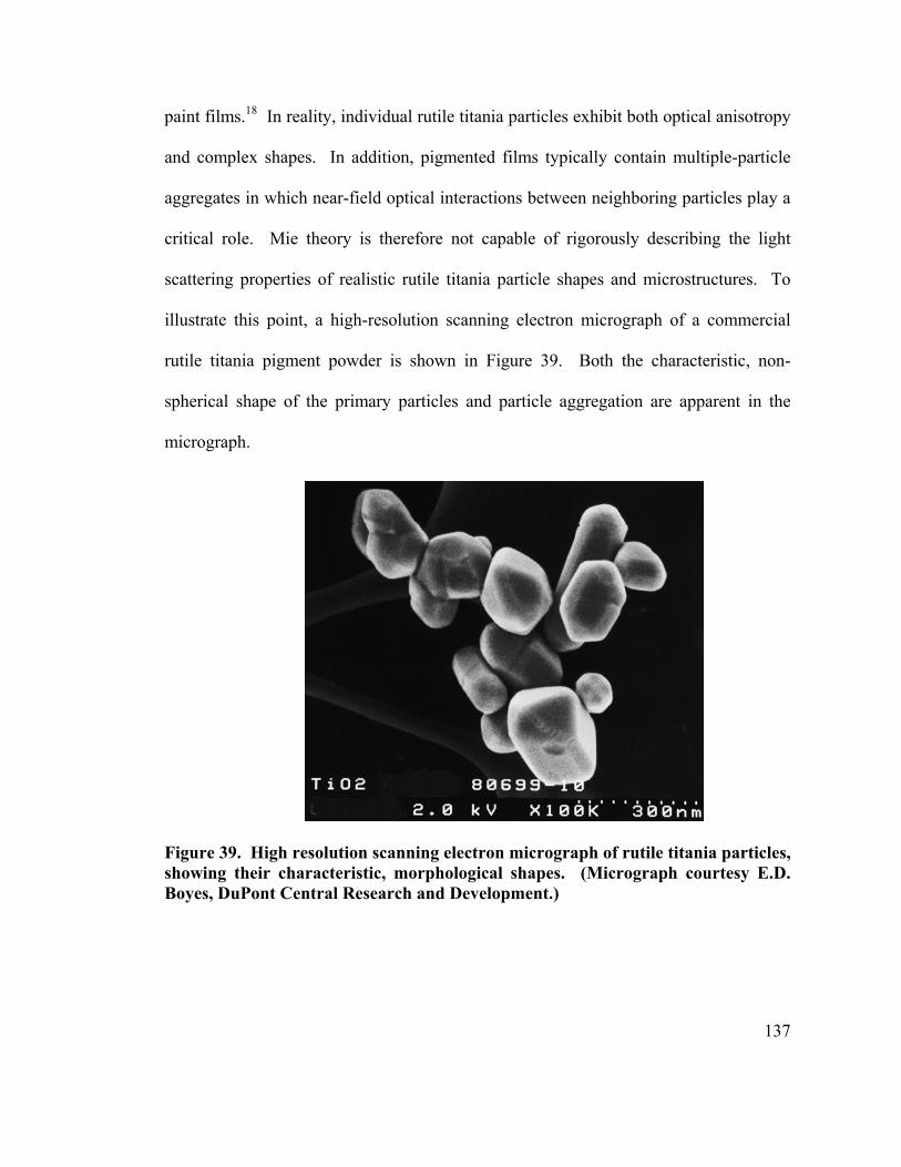
137

paint films.18 In reality, individual rutile titania particles exhibit both optical anisotropy

and complex shapes. In addition, pigmented films typically contain multiple-particle

aggregates in which near-field optical interactions between neighboring particles play a

critical role. Mie theory is therefore not capable of rigorously describing the light

scattering properties of realistic rutile titania particle shapes and microstructures. To

illustrate this point, a high-resolution scanning electron micrograph of a commercial

rutile titania pigment powder is shown in Figure 39. Both the characteristic, non-

spherical shape of the primary particles and particle aggregation are apparent in the

micrograph.

Figure 39. High resolution scanning electron micrograph of rutile titania particles, showing their characteristic, morphological shapes. (Micrograph courtesy E.D. Boyes, DuPont Central Research and Development.)

138

5.3.2 Scattering by a Morphological Rutile Particle

Here, the time-domain finite element approach has been applied to the case of

560-nm light scattering by a single, morphological rutile titania particle . This particle,

shown in the upper panels of Figure 40, has a width 0.175 µm and a tip-to-tip length of

0.35 µm. The shape and size of this particle is representative of rutile titania pigment

and has been chosen to illustrate the scattering properties of a typical pigment particle.

In contrast to the finite element computations performed for the case of a single sphere

in the Section 3 of this study, this rutile particle has been assigned the appropriate

anisotropic optical constants. As in the calculations described above, the particle is

surrounded by a medium with refractive index n = 1.51, representative of an acrylic

resin. This model contains ~1.6 million cubic elements, 3.6 nm on edge. This

corresponds to a finite element mesh density of ρ = 50 elements per light wavelength in

the model. The upper left panel of Figure 40 shows a three-dimensional view of the

sphere with the surrounding medium hidden; the cubic elements which compose the

particle are visible. The upper right panel shows a cross-sectional view of the finite

element model, including the particle and the surrounding medium. In this case, light is

propagating in the finite element model with components in both the +x and +z

directions with unit incident intensity. The lower two panels of Figure 40 show

scattered intensities in the geometric domains displayed in the corresponding upper

panels. As in the case of the spherical particle shown in Figure 10, scattered intensities

in the near field can be several times greater than the incident intensity.

139

In general, the rutile titania particles in a paint film are randomly oriented. In

order to determine the light scattering properties of the morphological, anisotropic rutile

particle shown in Figure 40 under conditions of diffuse illumination, a set of individual

finite element computations with different angles of light incidence are performed.

Two individual plane waves having mutually perpendicular polarizations are used for

each illumination direction. To determine far-field scattering properties under

conditions of random illumination, far-field intensities for the individual illuminations

are superimposed. The presence of four different mirror planes in the spatial symmetry

of the rutile particle shown in Figure 40 requires that only one half-octant of the particle

be illuminated to determine the full light scattering properties of the particle. In the

present case, fifteen different illumination directions were employed over one half-

octant of the particle, which is equivalent to one hundred eighty illumination directions

over the entire particle. Using the finite element method, the far-field scattering

parameters S = 23.97 µm−1 and σ = 10.07 µm−1 have been computed for the rutile

particle shown in Figure 40.

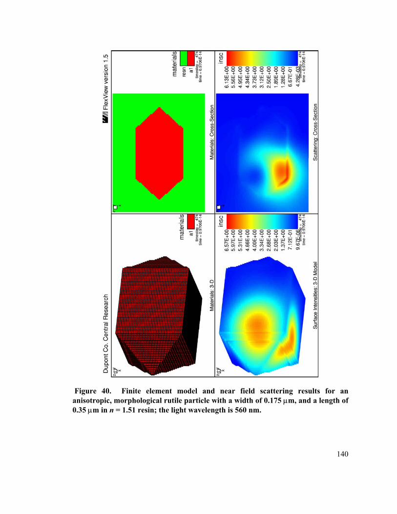
140

Figure 40. Finite element model and near field scattering results for an anisotropic, morphological rutile particle with a width of 0.175 µm, and a length of 0.35 µm in n = 1.51 resin; the light wavelength is 560 nm.

141

5.3.3 Discussion

5.3.3.1 Scattering Coefficients of the Morphological Rutile Particle

It is of interest to compare the far-field scattering parameters S and σ computed

for the rutile particle to those from Mie theory for the sphere with equivalent volume,

using both the average index and weighted sum approximations. The volume of the

rutile particle shown in Figure 40 is 7.77x10-3 µm3, corresponding to an equivalent

spherical diameter of 0.246 µm. Such comparisons provide a sense of the adequacy of

Mie theory to describe the optics of realistic rutile particles. Table 7 shows the results

of this comparison, with S and σ values shown for the finite element computation for

the rutile particle and for the equivalent volume sphere computed using both the

average index and weighted sum approximations. For the average index approximation,

the S result is 1.4% lower than the finite element result, and the angle-weighted

scattering coefficient σ result is 4.6% higher than the finite element result. For the

weighted sum approximation, the S result is 6.4% lower than the finite element result,

and the angle-weighted scattering coefficient σ is in agreement with the finite element

result. For this particular rutile particle, at least, the scattering properties of the

equivalent volume sphere computed using the two approximations and Mie theory are

within ~5% of the finite element result.

142

5.3.3.2 Mie Theory in Particle Size Analysis by Light Scattering

It is common practice in particle sizing methods based upon light scattering to

use Mie theory to compute particle size distributions for particles which are in reality

non-spherical.2 In these methods, the light scattering properties of a system are used to

determine equivalent spherical particle sizes by fitting scattering data to a size

distribution. It is therefore of considerable interest to compare the results of the finite

element calculations on systems containing realistically shaped rutile particles to the

results of Mie theory. This can be achieved by back-calculating equivalent spherical

diameters corresponding to the morphological rutile particle based upon the scattering

parameters S and σ rather than upon particle volume (as in Table 7).

Using the results S = 23.97 µm−1 and σ = 10.07 µm−1 for the isolated rutile

particle shown in Figure 40, the Mie theory results shown in Figure 31−Figure 34 have

been used to compute the spherical diameters exhibiting these same far-field scattering

parameters. These results are shown in Table 8. For both the average index and

weighted sum approximations, four different spherical diameters correspond to

matching S values, and two different spherical diameters correspond to matching angle-

weighted scattering coefficient σ values. The multiple sphere diameters corresponding

to the single S and σ values associated with this particle result from multiple

occurrences of these values in the curves shown in Figure 31−Figure 34. These results

highlight the potential ambiguity in using Mie theory to impute equivalent spherical

diameters to non-spherical particles based upon far-field scattering properties.

143

Table 7. Comparison between the far-field scattering coefficients for the single rutile particle and the equivalent volume sphere, using both the average index

and weighted sum approximations.

S (µm−1) σ (µm−1)

Anisotropic Rutile Particle

w=0.175 µm, Aspect Ratio 2

23.97 10.07

Equivalent-Volume Sphere n = 2.74

22.44 10.07

Equivalent-Volume Sphere Weighted Sum of n=2.64 and

n = 2.94 Results

23.64 10.54

Table 8. Diameters of spheres exhibiting the same far-field scattering coefficients as the single rutile particle, using both the average index and

weighted sum approximations.

S Basis σ Basis

Equivalent Spherical Diameter n = 2.74

0.186 µm or 0.212 µm

or 0.254 µm

or 0.293 µm

0.183 µm

or 0.247 µm

Equivalent Spherical Diameter

Weighted Sum of n = 2.64 and n = 2.94 Results

0.190 µm or 0.204 µm or 0.248 µm

or 0.287 µm

0.179 µm

or 0.261 µm

144

1 L.L Houle, J. Boudreau, and G. Shukla, TAPPI 1990 Coating Conference Proceedings, TAPPI Press, Atlanta (1990). 2 R.A. Kwoka, TAPPI 1990 Dyes, Fillers and Pigments Short Course, TAPPI Press, Atlanta (1990). 3 R.A. Kwoka, TAPPI 1993 Coating Conference Proceedings, TAPPI Press, Atlanta (1993). 4 R.A. Kwoka, and T.W. Logan, TAPPI Journal, 77 (10), 136 (1994). 5 Y. Wang, “Local Field Effect in Small Semiconductor Clusters and Spheres,” J. Phys. Chem., 95 (3), 1119-1124 (1991). 6 J.G. Balfour, “Opacity and Titanium Dioxide Pigments,” J. Oil Colour Chem. Assoc., 73, 225 (1990) 7 D.F. Tunstall and M.J. Hird, “Effect of Particle Crowding on Scattering Power of TiO2 Pigments,” J. Paint Technol., 46, 33-40 (1974).

145

Chapter 6. Clusters of Latex Spheres: A Low-Contrast System

This chapter describes the light scattering properties of clusters of latex particles

in water studied using the time-domain finite element method. Using synthesis methods

such as emulsion polymerization, polymeric materials can be formed as sub-micron

latex particles which are spherical in shape and can be nearly monodisperse in size. The

use of latex particles is widespread in polymer processing, since these materials can be

readily dispersed in liquids and subsequently formed into complex shapes. Latex

particles can be stabilized in water, allowing the elimination of potentially flammable

and toxic volatile organic solvents from the processing of the sol. This valuable

attribute of latices has created a very large market for latex-based paint systems. The

near monodispersity and controllable dispersion characteristics of latex systems makes

them ideal for model studies of particle agglomeration dynamics in liquid suspensions.

These agglomeration characteristics can be studied by microscopy, rheological

measurements, and light scattering techniques.

In Section 6.1, the general scattering properties of the materials system of

interest are described. In Section 6.2, the effects of latex particle agglomeration upon

the scattering properties of the system are described. In Section 6.3, the length scale

over which near-field optical interactions between neighboring latex particles are

determined. The computational results presented in this chapter are placed within the

context of scattering efficiency and hiding power. The latex system studied here is of

particular interest because it is a widely used system with low optical contrast,

146

providing a valuable basis for comparison with the results for clusters of white pigment

particles with high optical contrast described in Chapter 7.

6.1 Materials System of Interest

The system of interest in the present work is a latex material with refractive

index n = 1.50 in a water medium with refractive index n = 1.33. The illuminating

wavelength is 488 nm, a commonly used argon ion laser wavelength. A plot of the

scattering coefficient S versus diameter for a single sphere calculated using Mie theory

for these conditions is shown in Figure 41. The sphere diameter producing the

maximum S value is 1.4 µm. The low optical contrast of this system produces

significantly lower S values (one order of magnitude) than the high-contrast pigment

particle systems studied in the previous chapter. A plot of the angle-weighted scattering

coefficient σ versus sphere diameter calculated using Mie theory for the latex system is

shown in Figure 42. The sphere diameter producing the maximum σ value is 0.18 µm.

This value is significantly smaller than the 1.4 µm diameter producing the maximum S

value in Figure 41. This result indicates that the quantity (1−g), where the asymmetry

parameter g is the average cosine of the scattering angle, decreases sharply with

increasing sphere diameter in the sub-micron size range. That is, there is a rapid

transition from isotropic to forward scattering as the latex particle size increases beyond

the Rayleigh regime. The primary particle size studied here is 200 nm, a representative

latex particle diameter. This sphere diameter is indicated in the plots of Figure 41 and

Figure 42 with an “x”; this particle size provides an especially interesting case since it is

147

sub-optimal for the scattering coefficient S and very nearly optimal for the angle-weight

scattering coefficient σ.

The light scattering properties of a single 200-nm latex sphere in water has been

computed using the time-domain finite element method. Shown in Figure 43 are the

model geometry and near field scattered intensities for this computation. The 488-nm

light propagates in the +x direction and is polarized in the z direction. The top two

panels of this figure show a three-dimensional view of the scattering sphere and a cross-

sectional slice through the center of the model, respectively. The bottom two panels of

this figure show the near-field scattered intensities as a function of position in the

geometries shown in the top two panels. In contrast with the titania sphere in resin

shown in Figure 10, the latex sphere shown in Figure 43 exhibits scattered intensities in

the near field which are much smaller than the unit intensity of the incident light. This

is a result of the relatively low optical contrast of the latex system. The distribution of

scattered light in Figure 43 shows that most of the light is scattered in the forward

direction, with two lobes of concentrated light on the forward-scattering hemisphere of

the particle. The computed values of the scattering coefficients S and σ from the results

shown in Figure 43 are within 0.8% and 0.9% of the exact results computed from Mie

theory, respectively, showing close agreement.

148

0

.5

1

1.5

2

2.5

3

3.5

0 .5 1 1.5 2 2.5 3 3.5 4

S

Sphere Diameter (Microns)

( m

)

µ−1

x

Figure 41. The scattering coefficient S as a function of sphere diameter for a latex particle with n = 1.50 in a water medium with n = 1.33. The illuminating light wavelength is 488 nm. The 200-nm sphere diameter studied in this chapter is marked with an “x.”

0

.05

.1

.15

.2

.25

0 .5 1 1.5 2 2.5 3 3.5 4

σ

Sphere Diameter (Microns)

( m

)

µ−1

x

Figure 42. The angle-weighted scattering coefficient σ as a function of sphere diameter for a latex particle with n = 1.50 in a water medium with n = 1.33. The illuminating light wavelength is 488 nm. The 200-nm sphere diameter studied in this chapter is marked with an “x.”

149

Figure 43. Finite element model for a 200-nm latex sphere with n = 1.50 in a water medium with n = 1.33. The illuminating wavelength is 488 nm, and light propagates in the +x direction.

150

6.2 Light Scattering by Latex Sphere Clusters of Increasing Size

A series of computations has been performed using the time-domain finite

element method to determine the light scattering properties of particle clusters

containing increasing numbers of the 200-nm primary particle shown in Figure 43.

Cluster sizes investigated consisted of 2, 3, 6, 7, 8, 13, 27 and 64 primary particles. The

packings of these particles are not identical in each case; instead, the highest-symmetry

arrangements have been selected. For example, the clusters of 8, 27, and 64 spheres

share a simple cubic packing, while the cluster of 13 spheres has a face-centered cubic

packing. The geometries of the clusters containing 3, 7, 13, and 27 spheres are shown

in Figure 44 as examples of the cluster packings. In each computation, random

illumination conditions are simulated using the Illuminator software, yielding

orientation-averaged scattering coefficients along with the individual scattering results

for each illumination direction and polarization.

Near-field optical interactions between the latex spheres in these clusters can be

expected to occur and thus produce light scattering properties which differ from those

of the isolated, 200-nm latex primary particle which composes each cluster. The finite

element method permits direct visualization of these near-field interactions. Shown in

Figure 45 are geometric views of the cluster containing seven 200-nm latex particles

and the distribution of scattered light intensity in the near field. The top two panels of

this figure show a three-dimensional view of the spheres and a cross-sectional slice

through the center of the model, while the bottom two panels show the distribution of

151

scattered light through these two geometric views. The geometry of this model consists

of a central sphere surrounded by two neighboring spheres along each of the three axes

of the Cartesian coordinate system. As in all of the sphere clusters constructed in this

study, the spheres are in hard contact with their neighbors. The 488-nm light

propagates in the +x direction in the computation shown in Figure 45. The lower two

panels of Figure 45 demonstrate clearly that near-field scattered light in the seven-

sphere cluster is not distributed evenly among the seven primary particles in the cluster

as would be the case in the limit of single scattering. Instead, the greatest intensity of

scattered light is in the forward-scattering hemisphere of the cluster. This result is

significant and illustrates a phenomenon which is observed in all computations

performed on these latex sphere clusters: a cluster of latex spheres scatters light as a

single entity rather than as a collection of independent particles. This fact lies at the

root of the dramatic effects of sphere clustering upon light scattering which are

described in this and the following sections of this chapter.

The effects of latex particle clustering upon the scattering coefficient S are

shown in Figure 46 with S plotted as a function of the number of spheres contained in a

cluster. There is a steady increase in S as additional particles are added to the cluster.

A discontinuity occurs for the case of the seven-sphere cluster; this is likely due to the

relatively low packing density of this cluster (see Figure 45) compared to the others.

The S results shown in Figure 46 indicate that the efficiency of light scattering by these

latex clusters increases on a volume-normalized basis with increasing numbers of

primary particles in a cluster. The value of S for a six-sphere cluster is two times that

152

associated with a single latex primary, for example, and the value for a sixty-four-

sphere cluster is nearly four times that associated with the isolated primary.

The quantity (1−g) is plotted in Figure 47 as a function of the number of latex

spheres in a cluster. The data indicate a sharp decrease in this term as cluster size

increases, corresponding to a decrease in the fraction of light deflected away from the

forward-scattered direction. This decrease in (1−g) is the opposite of the trend observed

in the scattering coefficient S. That is, while clustering of greater numbers of the 200-

nm latex spheres causes increased scattered intensity on a volume-normalized basis, this

additional scattered intensity is directed more strongly in the forward direction. The

opacifying efficiency of these clusters in an aqueous dispersion depends upon the angle-

weighted scattering coefficient σ, which is the product of S and (1−g). The opposite

trends observed in S and (1−g) indicate that the dependence of σ upon the number of

spheres in a cluster is less strong than the case of either S or (1−g).

The effects of latex particle clustering upon the scattering coefficient σ are

shown in Figure 48 with σ plotted as a function of the number of spheres contained in a

cluster. In contrast to the results of Figure 46 for the scattering coefficient S, the plot in

Figure 48 in general shows a steady, but only slight, decrease in σ with increasing

numbers of latex spheres in a cluster. The global maximum in the data corresponds to

the case of a two-sphere cluster, exhibiting a σ value which is 5% greater than that of

the isolated latex primary. For larger clusters, there is little change in the data between

the cases of 13-, 27-, and 64-sphere clusters. The cluster of thirteen particles exhibits a

153

σ value which is 25% lower than that associated with the isolated latex primary, and

the cluster of sixty-four primary particles exhibits a value which is about 15% lower

than the isolated latex primary. It can be concluded that, in general, clustering of these

latex spheres over the size range investigated here results in poorer scattering efficiency

for a dispersion of these particles compared to the case where no particle agglomeration

is present.

154

Figure 44. Finite element models of latex sphere clusters containing 3, 7, 13, and 27 spheres.

155

Figure 45. Finite element model of a cluster of seven 200-nm latex spheres n = 1.50 in a water matrix with n = 1.33. The 488-nm illuminating light propagates in the +x direction and is polarized in the z direction.

156

Number of Spheres0 10 20 30 40 50 60 70

S (µ

m-1

)

0.0

0.5

1.0

1.5

2.0

Figure 46. The scattering coefficient S as a function of the number of 200-nm latex particles composing a particle cluster under conditions of random illumination.

Number of Spheres0 10 20 30 40 50 60 70

(1-g

)

0.0

0.1

0.2

0.3

0.4

0.5

Figure 47. The quantity (1−g) as a function of the number of 200-nm latex spheres composing a particle cluster under conditions of random illumination.

157

Number of Spheres0 10 20 30 40 50 60 70

σ (µ

m-1

)

0.0

0.1

0.2

0.3

Figure 48. The scattering coefficient σ as a function of the number of 200-nm latex spheres composing a particle cluster under conditions of random illumination.

6.3 Near-Field Interactions Between Neighboring Latex Particles

In the previous section, it has been demonstrated that clusters of 200-nm latex

spheres can exhibit substantially different scattering efficiencies than the individual

primary particles composing them. That result calls into question of the length scale of

interparticle separation over which near-field interactions between the particles are

important. In this section, this question is investigated in model systems containing a

small number of 200-nm latex particles illuminated with 488-nm light. These model

systems are based upon the geometry of the seven-sphere cluster shown in Figure 45;

the spacing between the central sphere and the six surrounding spheres are uniformly

varied from one computation to the next. In the case of a 0.4-µm interparticle

separation, for example, each of the six surrounding spheres is positioned to have a 0.4-

158

µm surface-to-surface interparticle separation from the central sphere. The resulting

shape of the cluster is therefore an octahedron for each interparticle separation distance

investigated. Conditions of random illumination are simulated for each separation

distance using the Illuminator software, and scattering efficiencies are computed on an

orientation-averaged basis as in Section 6.2.

The geometry of the model with 0.4-µm surface-to-surface interparticle

separation distance is shown in Figure 49. The upper two panels of this figure show a

three-dimensional view of the latex spheres and a cross-sectional slice through the

center of the finite element model. Five of the spheres in the seven-sphere cluster are

bisected by this cross-sectional slice; the other two particles are positioned in the +z and

–z directions in the model (out of the page, and into the page, respectively). Shown in

the lower two panels are the distributions of near-field scattered light intensity on the

surfaces of the seven spheres and through the cross-sectional slice through the center of

the model. The incident 488-nm light is polarized in the z-direction in this computation

and propagates in the +x direction in the model. There are several interesting features

in the distributions of scattered light intensity in the near field for this computation.

First, it is clear in both the surface and cross-sectional views that each of the seven

individual latex spheres do not exhibit the same distribution of scattered light on their

surfaces or through their cross-sections. Instead, the two spheres positioned in the

forward scattering (+x) direction appear to have greater scattered intensities in their

immediate vicinity than the other spheres in the cluster. This suggests that at this 0.4-

µm separation, the seven particle are interacting optically in the near field rather than

159

scattering independently. This interaction is evident in the scattered intensity

distribution in the cross-sectional slice through Figure 49, in which faint scattered

intensity is visible in the spaces between the five particles visible in that view. It is also

interesting to compare the results for 0.4-µm interparticle separation distance in Figure

49 with those for the touching spheres in Figure 45. It is evident that while the seven

spheres separated by 0.4 µm do not scatter light independently, the distribution of

scattered light between those spheres is more even than the distribution of scattered

light in the cluster of touching spheres. That is, these near-field results suggest that the

light scattering properties of the cluster with 0.4-µm interparticle separation should be

much closer to the result for seven isolated spheres than the case of the cluster of seven

touching spheres.

The dependence of the scattering coefficient S upon surface-to-surface

interparticle separation distance for the clusters of seven latex spheres is shown in

Figure 50. The dashed line in this plot corresponds to the S value associated with a

single, isolated 200-nm latex primary particle. Deviations from this dashed line are the

result of near-field interactions between neighboring spheres in the clusters. At the

maximum interparticle separation distance studied, 0.6 µm, the S value exhibited by the

seven-sphere cluster is only 5% greater than that of a single 200-nm latex primary

particle. The data in Figure 50 indicate a steady increase in S as the interparticle

spacing between the spheres in the cluster decreases to zero. For the case of zero

interparticle separation distance (touching spheres, Figure 45), the value of S is 0.88

µm-1, which is 80% greater than the value associated with a single primary particle.

160

(This case is part of the data set shown in Figure 46.) The interparticle separation

distance at which the seven-sphere cluster exhibits an S value more than 10% greater

than that of an isolated 200-nm primary particle is 0.35 µm, which is very close to the

effective wavelength of the 488-nm light in water with n = 1.33 refractive index.

The quantity (1−g) is plotted in Figure 51 as a function of interparticle

separation distance between the seven-sphere clusters. The dashed line in the plot

indicates the value associated with a single 200-nm latex primary particle. As in the

case of particle agglomeration investigated in Section 6.2, the quantity (1−g) exhibits

the opposite trend from the scattering coefficient S, decreasing sharply as the

interparticle separation distance approaches zero. That is, as the seven spheres in these

clusters approach each other and interact more strongly optically, the total amount of

light scattering increases but this scattered intensity is directed more strongly in the

forward direction. The value of (1−g) for the case of touching spheres is 46% lower

than that of a single 200-nm latex primary particle.

The dependence of the angle-weighted scattering coefficient σ upon interparticle

separation distance in the seven-sphere clusters is shown in Figure 52. As in Figure 50

and Figure 51, the dashed line in this figure corresponds to the value associated with a

single 200-nm latex primary particle. The data indicate a relatively weak dependence of

σ upon interparticle separation distance, compared to either S or (1−g). The value

associated with zero interparticle separation is just 5% less than that associated with a

single 200-nm latex primary particle. In contrast to the data for S and (1−g), the σ data

161

oscillate about the value associated with the single latex primary particle, exceeding it

by about 3% with a 0.25-µm interparticle separation distance. The data appears to have

an oscillatory character, but the amplitude of this oscillation is not large compared to

the 1-3% error level expected in these computations.

162

Figure 49. Finite element model of a cluster of seven 200-nm latex spheres n = 1.50 in a water matrix with n = 1.33. The surface-to-surface interparticle spacing is 0.4 µm. The 488-nm illuminating light propagates in the +x direction and is polarized in the z direction.

163

0.0 0.1 0.2 0.3 0.4 0.5 0.60.4

0.5

0.6

0.7

0.8

0.9

Separation (µm)

S ( µ

m-1

)

Figure 50. Dependence of the scattering coefficient S upon surface-to-surface interparticle separation distance for the clusters of seven latex spheres. The dashed line corresponds to the value associated with a single 200-nm latex primary particle.

Separation (µm)0.0 0.1 0.2 0.3 0.4 0.5 0.6

(1-g

)

0.2

0.3

0.4

0.5

0.6

Figure 51. Dependence of the quantity (1−g) upon surface-to-surface interparticle separation distance for the clusters of seven latex spheres. The dashed line corresponds to the value associated with a single 200-nm latex primary particle.

164

Separation (µm)0.0 0.1 0.2 0.3 0.4 0.5 0.6

σ ( µ

m- 1

)

0.22

0.23

0.24

0.25

0.26

Figure 52. Dependence of the angle-weighted scattering coefficient σ upon surface-to-surface interparticle separation distance for the clusters of seven latex spheres. The dashed line corresponds to the value associated with a single 200-nm latex primary particle.

165

Chapter 7. Clusters of Titania Particles: A High-Contrast System

Chapters 2 and 5 have emphasized the technological importance of the light

scattering properties of high-index white pigment particles. The present chapter

describes the effects of near-field interactions between white pigment particles upon

scattering efficiency in several different systems. As stated previously, optical

interactions between neighboring white pigment particles are known to have profound

impact in end-use applications, yet the fundamental aspects of these phenomena have

not been directly studied successfully. In Section 7.1, the general scattering properties

of the materials system of interest are established. In Section 7.2, the effects of

clustering primary pigment particles which are optimized for scattering efficiency is

described. In Sections 7.3 and 7.4, the magnitude of near-field interactions between

separated particles is investigated for the cases of a seven-sphere cluster and of two

morphological rutile particles, respectively.

7.1 Materials Systems of Interest

In Sections 7.2 and 7.4, the results of studies upon the light scattering properties

of systems of multiple 200-nm spheres of high-index material are described. The

system investigated is that of a high-index material (n = 2.74) embedded in a medium

with index of refraction n = 1.51. The light wavelength studied is 560 nm. This system

is representative of rutile titania spheres using the average index approximation. The

sphere diameter studied here, as in the case of the latex system in the previous chapter,

166

is 200 nm. A plot of the scattering coefficient S versus diameter for a single sphere

calculated using Mie theory is shown in Figure 53. The sphere diameter producing the

maximum S value of 28 µm-1 is 0.3 µm. A plot of the angle-weighted scattering

coefficient σ versus diameter for a single sphere calculated using Mie theory is shown

in Figure 54. The sphere diameter producing the maximum σ value of 12.1 µm-1 is 0.2

µm. The 200-nm rutile sphere diameter studied here is indicated in each of these two

plots with an “x”. The 200-nm diameter studied here is that corresponding to the

maximum of the first resonant peak in S in the plot shown in Figure 53. In addition, this

sphere diameter produces the maximum σ value for this materials system. This particle

size may therefore be expected to produce qualitatively different behaviors upon

clustering than the 200-nm latex sphere studied in the previous chapter.

The light scattering properties of the single 200-nm rutile sphere under these

conditions has been computed using the time-domain finite element method; these

results are shown in Figure 10. A comparison of the near-field scattered intensities in

Figure 10 with those of the single latex sphere shown in Figure 43 indicates that the

main difference between these two systems is the much higher scattered intensities in

the vicinity of the titania sphere in Figure 10. Indeed, these near-field scattered

intensities are about 50 times higher than in the case of the latex particle. It is the

greater optical contrast between the titania particle and its surrounding medium,

combined with the resonant diameter of the titania sphere, which produces this stronger

scattering interaction.

167

0

5

10

15

20

25

30

0 .2 .4 .6 .8 1

S

Sphere Diameter (Microns)

( m

)

µ−1

x

Figure 53. The scattering coefficient S as a function of sphere diameter for a rutile particle with n = 2.74 in a polymer medium with n = 1.51 under the average index approximation. The illuminating light wavelength is 560 nm. The 200-nm sphere diameter studied in this chapter is marked with an “x.”

0

2

4

6

8

10

12

0 .2 .4 .6 .8 1

σ

Sphere Diameter (Microns)

( m

)

µ−1

x

Figure 54. The angle-weighted scattering coefficient σ as a function of sphere diameter for a rutile particle with n = 2.74 in a polymer medium with n = 1.51 under the average index approximation. The illuminating light wavelength is 560 nm. The 200-nm sphere diameter studied in this chapter is marked with an “x.”

168

7.2 Light Scattering by Titania Sphere Clusters of Increasing Size

As in the case of the latex particles in the previous chapter, a series of

computations has been performed using the time-domain finite element method to

determine the light scattering properties of particle clusters containing increasing

numbers of the 200-nm rutile sphere shown in Figure 10. Cluster sizes investigated

consisted of 2, 3, 4, 6, 7, 8, 13, 20, 27 and 64 primary particles. The same geometrical

packings used in the case of the latex particles have been used here. In each case,

random illumination has been simulated using the Illuminator software, yielding

orientation-averaged scattering coefficients along with the individual scattering results

for each illumination direction and polarization.

Shown in Figure 55 are geometric views of the cluster containing seven titania

particles and the distribution of scattered light in the near field. (Figure 45 shows the

analogous case for latex particles). The top two panels show a three dimensional view

of the spheres and a cross-sectional slice through the center of the model, while the

bottom two panels show the distribution of scattered light at steady state through these

two geometric views. The 560-nm light propagates in the +x direction in this case. As

in the case of the clustered latex spheres, the results in Figure 55 show that the

distribution of scattered light through the seven-sphere cluster is not uniform. Instead

the greatest concentration of scattered light is in the forward-scattering hemisphere of

the cluster. The incident light intensity for the computation shown in Figure 55 is unity.

In the lower two panels of this figure, the maximum scattered intensities observed are

therefore about 9 times higher than the incident intensity, indicating that the titania

169

cluster focuses scattered light in the forward direction. A comparison of near-field

scattered intensities observed for the seven-sphere cluster of titania spheres with those

observed for the single primary particle (Figure 10) indicate scattered intensities which

are about 3 times higher for the cluster.

The effects of titania particle clustering upon the scattering coefficient S are

shown in Figure 56 with S plotted as a function of the number of spheres contained in a

cluster. There is an increase in S by about 15% as a second sphere is added to the first,

and then a dramatic decrease in general as more particles are added to the cluster. The S

value associated with the thirteen-sphere cluster is 50% less than that associated with an

isolated primary particle, and the value associated with the sixty-four sphere cluster is

about 75% less than that of the isolated primary. In general, clustering of 200-nm

titania spheres results in markedly reduced total scattering on a volume-normalized

basis compared to the case of the isolated primary.

The effects of titania particle clustering upon the angle-weighted scattering

coefficient σ are shown in Figure 57 with σ plotted as a function of the number of

spheres contained in a cluster. These σ results share the same characteristic as the S

data in Figure 56, which is a pronounced decrease with increasing cluster size.

Contrary to the S results, the σ results in Figure 57 do not show an increase as the

cluster size is increased from one to two spheres. In addition, the decrease in σ

observed for small cluster sizes (<10 spheres) in Figure 57 with increasing cluster size

is more pronounced than the decrease in S in Figure 56 over the same size range. The

loss in σ for a four-sphere cluster is about 30% compared to the isolated primary

170

particle, while a loss in S of only about 10% occurs for this cluster. Similar losses in the

two coefficients S and σ occur for clusters larger than 10 spheres. The loss in σ for the

thirteen-sphere cluster is 60% compared to the isolated primary, and the loss associated

with the sixty-four sphere cluster is 70%. These results for titania spheres indicate that

the quantity (1−g) decreases rapidly with increasing cluster size for small clusters and

changes more slowly for large clusters.

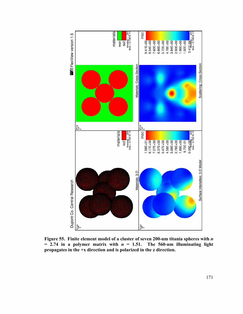
171

Figure 55. Finite element model of a cluster of seven 200-nm titania spheres with n = 2.74 in a polymer matrix with n = 1.51. The 560-nm illuminating light propagates in the +x direction and is polarized in the z direction.

172

0 10 20 30 40 50 60 70

S ( µ

m-1

)

0

5

10

15

20

25

30

35

Number of Spheres

Figure 56. The scattering coefficient S as a function of the number of 200-nm titania spheres composing a particle cluster. These results are for the case of random illumination of each cluster, resulting in orientation-averaged results.

Number of Spheres0 10 20 30 40 50 60 70

σ (µ

m-1

)

0

2

4

6

8

10

12

Figure 57. The scattering coefficient σ as a function of the number of 200-nm titania spheres composing a particle cluster. These results are for the case of random illumination of each cluster, resulting in orientation-averaged results.

173

7.3 Near-Field Interactions Between Neighboring Titania Particles

In the previous section, the effects of cluster sizes of 200-nm titania spheres

upon scattering efficiency has been studied using the time-domain finite element

method. In the present study, the effects of crowding are investigated for the case of the

seven-sphere cluster shown in Figure 55 by varying the interparticle separation distance

between the center sphere and the six surrounding spheres in the cluster. The surface-

to-surface interparticle separation distance is allowed to vary from zero to 0.5 µm. This

study is analogous to the study of crowding of latex spheres with this same geometry in

Section 6.3.

The dependence of the scattering coefficient S upon interparticle separation

distance in these seven-sphere clusters of titania is shown in Figure 58. The horizontal,

dashed line in this figure indicates the S value associated with a singe, isolated 200-nm

titania sphere of which the cluster is composed. The plot in Figure 58 shows that the S

values for the seven-sphere clusters is nearly equal to that of the isolated titania sphere

(within ~3%) for interparticle separation distances greater than 0.2 µm. The S values

for those clusters with interparticle separation distances greater than 0.4 µm in face

exceed the value associated with an isolated titania sphere by about 2%; this difference

is within the expected error for those computations and may be a result of numerical

error. For interparticle separation distances less than 0.2 µm, the scattering coefficient S

decreases very sharply with decreasing interparticle separation distance. For the case of

touching spheres (zero interparticle separation distance), the value of S is 16% lower

than the value associated with an isolated titania sphere. This 16% loss in the total

174

scattering by the cluster on a volume-normalized basis is the same value indicated in the

Figure 56 for the seven-sphere cluster.

The dependence of the angle-weighted scattering coefficient σ upon interparticle

separation distance in the seven-sphere clusters of titania is shown in Figure 59. The

horizontal, dashed line corresponds to the σ value associated with an isolated 200-nm

titania sphere of which the cluster is composed. The plot in Figure 59 shows that the

value of σ for the seven-sphere cluster with 0.5-µm surface-to-surface interparticle

separation distance is very nearly equal to that associated with an isolated 200-nm

titania sphere. The σ value at this separation distance is about 1.5% less than that of the

isolated primary particle, which is within the range of expected numerical error for this

computation. For interparticle separation distances less than 0.5 µm, the value of σ for

these seven-sphere clusters of titania decreases steadily as the separation distance

approaches zero. For a surface-to-surface interparticle separation distance of 0.2 µm,

the value of σ is 10% less than the value associated with an isolated sphere. For the

cluster of seven touching spheres, the value of σ is 35% less than the value associated

with an isolated sphere, indicating a substantial loss in scattering efficiency a result of

particle crowding and agglomeration in this system.

175

0.0 0.1 0.2 0.3 0.4 0.521

22

23

24

25

26

27

Separation (µm)

S (µ

m-1

)

Figure 58. Dependence of the scattering coefficient S upon surface-to-surface interparticle separation distance for the clusters of seven titania spheres. The dashed line corresponds to the value associated with a single 200-nm titania primary particle.

Separation (µm)0.0 0.1 0.2 0.3 0.4 0.5

σ (µ

m- 1

)

7

8

9

10

11

12

13

Figure 59. Dependence of the angle-weighted scattering coefficient σ upon surface-to-surface interparticle separation distance for the clusters of seven titania spheres. The dashed line corresponds to the value associated with a single 200-nm titania primary particle.

176

7.4 Near-Field Interactions Between Two Morphological Rutile Particles

Time domain finite element computations have been performed for the case of

two morphological rutile titania particles which approach each other in a resin. In this

case, two particles with the same geometry and anisotropic optical properties as the

particle shown in Figure 40 are positioned within a finite element model with

interparticle separations ranging from 0.5 µm to 0 µm (touching). Cross-sectional

views of the finite element models are shown in upper panels of Figure 60−Figure 62,

and the logarithm of scattered intensity through the same cross section are shown in the

lower panels. In each of these figures, the illumination direction is perpendicular to the

plane of the cross sections shown, and the light polarization is parallel to the long axes

of the particles. Asymmetry in the near-field scattered intensities around each of the

particles is apparent in each of these figures, indicating that the two particles are

interacting at these separations.

Random illumination conditions have been simulated for each of the

interparticle separations investigated using the Illuminator software. The presence of

three mutually perpendicular mirror planes in the geometry of the finite element models

limited the number of illumination directions to twenty-five in one octant of the finite

element model. The scattering parameter S has been computed for this two-particle

system as a function of surface-to-surface interparticle separation distance. This result

is shown in Figure 63; the horizontal line indicates the value of the scattering coefficient

for a single morphological rutile particle (Figure 40) for comparison with the two-

particle results. The scattering coefficient S decreases with decreasing separation

177

between the two particles. For an interparticle separation of 0.5 µm, the scattering

coefficient is very nearly equal to that associated with the isolated particle. For the case

of zero interparticle separation, the value of the scattering coefficient S is 8% lower than

that associated with a single, isolated particle. That is, the two-particle aggregate

scatters 8% less total light than the isolated particle.

Results for the angle-weighted scattering coefficient σ for the two-particle

system are shown in Figure 64 as a function of the interparticle separation distance.

The horizontal line in the figure indicates the σ value associated with a single

morphological rutile particle (Figure 40). The results Figure 64 show that the value of

the angle-weighted scattering coefficient σ for the interparticle separation of 0.5 µm is

nearly equal to that associated with the isolated particle. For the case of the two

particles touching, the value is 20% lower, indicating that the two-particle aggregate is

significantly less effective in the limit of multiple scattering than the isolated particle.

As in the case of the isolated rutile particle, it is possible to determine the

diameters of spheres with equivalent far-field scattering properties for the case of two

interacting rutile particles described above. This case is especially interesting since the

total volume of scattering material remains constant as the two rutile particles approach

each other, yet the far-field scattering properties of the system change markedly as the

interparticle distance changes. These results are presented in Table 9, with the sphere

diameters producing the same values of the scattering coefficients S and σ as the two-

particle system for each of the interparticle separation distances considered. As in the

178

case of the single rutile particle, multiple values of S and σ occur for each of the

interparticle separation distances.

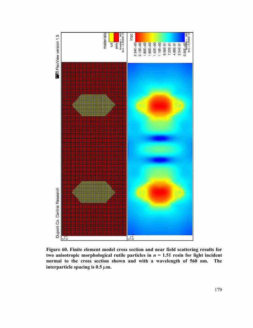
179

Figure 60. Finite element model cross section and near field scattering results for two anisotropic morphological rutile particles in n = 1.51 resin for light incident normal to the cross section shown and with a wavelength of 560 nm. The interparticle spacing is 0.5 µm.

180

Figure 61. Finite element model cross section and near field scattering results for two anisotropic morphological rutile particles in n = 1.51 resin for light incident normal to the cross section shown and with a wavelength of 560 nm. The interparticle spacing is 0.3 µm.

181

Figure 62. Finite element model cross section and near field scattering results for two anisotropic morphological rutile particles in n = 1.51 resin for light incident normal to the cross section shown and with a wavelength of 560 nm. The interparticle spacing is 0 µm.

182

0.0 0.1 0.2 0.3 0.4 0.5

22

23

24

S (µ

m-1

)

Separation (µm)

Figure 63. Scattering coefficient S for two morphological rutile particles as a function of interparticle separation. The horizontal line shows the results for one of the morphological rutile particles.

Separation (µm)0.0 0.1 0.2 0.3 0.4 0.5

σ (µ

m-1

)

8

9

10

Figure 64. Angle-weighted scattering coefficient σ for two morphological rutile particles as a function of interparticle separation. The horizontal line shows the results for one of the morphological rutile particles.

183

Table 9. Diameters of spheres exhibiting the same far-field scattering coefficients as the system of two rutile particles for each interparticle

separation distance considered, using both the average index and weighted sum approximations.

Interparticle Separation

(µm) S Basis σ Basis

0.5 0.186 0.211 0.254 0.292

0.183 0.278

0.4 0.186 0.212 0.254 0.293

0.183 0.279

0.2 0.184 0.215 0.252 0.295

0.181 0.285 0.337 0.349

0.1 0.182 0.22 0.249 0.297

0.178 0.295 0.328 0.354

0 0.180 0.228 0.242 0.301

0.171 0.360

184

Chapter 8. Discussion: Light Scattering by Complex Microstructures in the Resonant Regime

The light scattering properties of several previously unknown systems have been

determined computationally in this dissertation research. The results of these studies,

presented in Chapters 4−7, provide a basis for the elaboration of new insights about the

light scattering properties of complex microstructures. This chapter contains a

discussion of these learnings on a general footing.

8.1 Accuracy of the Time-Domain Finite Element Method

Studies have been presented in Chapter 4 upon the accuracy of the time-domain

finite element method with different finite element model configurations and far-field

extrapolation conditions. The methodology used in this work has been to systematically

vary computational conditions in the finite element method and compare the numerical

results to known, analytical results from Mie theory. The materials systems

investigated using Mie theory were as closely related to the more complex systems of

interest in subsequent research as possible. In each of the variations in computational

conditions studied, wide variations in the accuracy of the finite element method were

observed. It is significant that those computations which were grossly in error showed

no outward signs of any problem, such as crashes or error messages. Without the

foundations of understanding developed in the error analysis work, it would be

impossible to apply the time-domain finite element method to unknown cases with

confidence.

185

The explosion in computational power which has occurred in the late 1990’s has

created an unprecedented environment for successful application of computational

modeling to complex physical phenomena. This opening has been accompanied by the

development of diverse numerical methods in a given field, putting at one’s disposal

numerous approaches to the modeling of a given system. Each approach has its unique

advantages and disadvantages for the solution of a particular problem. In the field of

computational modeling and simulation (and in experimental work, for that matter),

there is an unfortunate tendency for researchers to vaunt the particular numerical

methods they develop or apply, at the expense of alternative approaches, and to avoid

discussion of their shortcomings. Careful and detailed studies of the accuracy of any

numerical method under the full range of computational conditions is critical, for it is

only through a sound understanding of the limitations of a numerical method that its

strengths can be appreciated.

8.2 Light Scattering by Complex, Resonant Particles

The light scattering properties of core-shell pigment particles illustrate important

principles about the design of complex particle architectures in the resonant regime. It

is well-known that the scattering of light arises from dielectric discontinuities between

different materials. It could therefore be argued that increased light scattering could be

produced by creating a large number of interfaces in an engineered composite particle.

One could imagine a complex particle consisting of a series of alternating, concentric

shell layers of high- and low-index materials; each interface in the particle would create

a source of light scattering, resulting in a particle with light scattering properties which

186

are superior to either of the constituent materials alone. In the case of the core-shell

particles studied in Chapter 5, which consist of a high-index titania shell surrounding

lower-index core materials, it has been demonstrated that this sort of approach is not a

viable means of producing pigment particles with superior light scattering properties in

the resonant regime. Instead, the core-shell architecture produces the same trends in

behavior as reducing the effective refractive index of the composite particle. Core-shell

particles with optimized diameter exhibit substantially lower scattering coefficients than

particles of the high-index material with optimized diameter. An explanation for these

observations lies in the relationship between the core-shell particle size and the

wavelength of the illuminating light. Since the core-shell particle diameters producing

optimal light scattering are on the order of the light wavelength in size, the potential for

increased light scattering by a multi-layer particle architecture is limited by the

resolution of the illuminating light. In simple terms, the light does not “see” the internal

particle interfaces so much as it “sees” a particle with reduced effective refractive index.

The strategy for producing white pigment particles with maximum light scattering

power is to produce optimally sized, solid particles of the highest refractive index, non-

absorbing material available.

The effects of optical anisotropy upon light scattering in the resonant regime

have been investigated for the first time in the study presented in Chapter 5. The results

of that study revealed the expected phenomena of orientation- and polarization-

dependent light scattering properties in the anisotropic spheres studied. Changes in the

scattering coefficients S by as much as 50% were demonstrated for different

187

illumination directions and light polarizations in the case of the highly resonant 0.2-µm

sphere. This orientation and polarization dependence is an essential difference between

the anisotropic spheres and the isotropic spheres considered in Mie theory. Calculation

of the scattering parameters S and σ on an orientation-averaged basis, on the other hand,

revealed that the scattering properties of anisotropic spheres can be approximated

reasonably, within 10%, by isotropic scattering models. The approximate formulations

do not describe the orientation-averaged scattering behavior of the anisotropic spheres

rigorously, but the errors were not dramatic. These results suggest that dilute ensembles

of optically anisotropic particles which are truly randomly oriented may be well

approximated using isotropic models which can be far less complex to analyze. They

also highlight the fact that there are potential opportunities to improve the scattering

properties of ensembles of anisotropic particles forcing the particles to adopt preferred

orientations during processing. For example, it is possible to deliberately align particles

with high aspect ratios during processing, which may be advantageous for light

scattering performance in certain systems.

Finite element computations on the light scattering properties of a single,

morphological rutile titania particle demonstrate the ready applicability of the method to

even the most complex particle shapes. This resonant particle is faceted and exhibits

anisotropic optical properties. The absence of cylindrical symmetry in the rutile particle

makes its scattering properties especially difficult to model using techniques like the T-

matrix method which are not based upon piece-wise solution of Maxwell’s equations

through a large system of volume elements. The computed light scattering properties of

188

the rutile particle have been compared to those of the equivalent-volume sphere using

two approximations based upon scattering by an isotropic sphere. As in the case of

anisotropic spheres, the isotropic scattering models were in reasonable statistical

agreement with the computed scattering coefficients of the rutile particle, with errors

less than 10% in all cases. It can be concluded that equivalent-volume, isotropic

spheres approximate reasonably the light scattering coefficients of complex single

particles in the resonant regime, but rigorous agreement is not achieved.

The computed coefficients S and σ of the morphological rutile particle were also

used to identify those isotropic sphere diameters producing the same scattering

coefficients. In this case, there were multiple sphere diameters in each case which

exhibited the same scattering coefficients. This study highlights the ambiguity of

assigning equivalent spherical diameters to particles with complex shapes and therefore

more degrees of freedom in their geometry than a simple sphere. Particle sizing

methods based upon light scattering and the assignment of equivalent spherical

diameters should be regarded as effective engineering control tools rather than absolute

measures of true particle size.

8.3 Light Scattering by Densely Packed Particle Aggregates

The light scattering coefficients of multiple-sphere clusters containing different

numbers of primary particles have been determined using the time-domain finite

element approach in two different materials systems. The first system, representing

clusters of 200-nm latex spheres in water (Chapter 6), is a low-contrast system in which

189

the refractive index ratio of the two materials is 1.13. The second system, representing

clusters of 200-nm titania spheres in a polymeric resin (Chapter 7), is a high-contrast

system in which the refractive index ratio of the two materials is 1.81. It is interesting

to note that, while 488-nm light was used in the case of the latex-water system and 560-

nm was used in the titania-resin system, the effective light wavelengths in the two

systems were nearly identical due to the different refractive indices of the water and the

resin. In the case of the latex-water system, the effective light wavelength is 488-

nm/1.33 = 367 nm. In the case of the titania-resin system, the effective light

wavelength is 560-nm/1.51 = 371 nm. The large difference in contrast ratio between

these two systems result in very different far-field scattering coefficients for the isolated

200-nm primary particle used to build the clusters in both cases (compare Figure 41-

Figure 42 with Figure 53-Figure 54.)

The results of computing the scattering coefficients of the packed particle

clusters studied in these two systems illustrate the fact that the multiple-particle clusters

exhibit very different scattering properties than the isolated primaries composing them.

In addition, the trends in the scattering coefficients S and σ as a function of the number

of 200-nm primaries in a cluster were in some cases opposite in these two materials

systems. That is, there exists no simple function which can be used to predict how the

scattering coefficients will change for clustering of arbitrarily sized primary particles in

an arbitrary materials system.

For the formation of multiple-particle clusters from a given primary particle size

and optical constants, an important consideration is the relationship between the

190

scattering coefficient S or σ of the isolated primary particle compared to the diameter

associated with the optimal value of that scattering coefficient. In other words, a critical

question is where the primary particle diameter is positioned on the computed scattering

coefficient curve from Mie theory. This knowledge provides the ability to predict in a

semi-quantitative way how the scattering coefficient of clusters of the primary particle

will trend with increasing cluster size. For example, for a primary particle diameter

which is much smaller than the diameter producing the maximum value of the angle-

weighted scattering coefficient σ in a given materials system, the formation of multiple-

particle clusters of increasing size will result in increased σ values. These increased σ

values, however, will not attain the value of the solid particle which is of optimal size in

the system. Likewise, for a primary particle diameter which is equal to that producing

the maximum σ value in a system, the formation of clusters of increasing size from that

primary particle will result in decreased σ values. It appears that this sort of

comparison is the only reliable means of predicting trends in scattering coefficients as a

function of the degree of particle clustering.

Comparisons are made here between the scattering properties of clusters

composed of arbitrary numbers of primary particles and the results of Mie theory

computations for single, equivalent-mass spheres. Shown in Figure 65 is a comparison

between values of the scattering coefficient S in the latex-water system as a function of

the number of spheres in a cluster (from Figure 46) and the results of Mie theory

computations for equivalent-mass spherical particles (dashed curve). The Mie theory

computations correctly predict the upward trend in S with increasing cluster size. In a

191

quantitative sense, however, the agreement between the two sets of data is statistically

poor for the largest cluster sizes investigated. For the cluster consisting of sixty-four

200-nm latex spheres, for example, the predicted value of S is 45% greater for the

equivalent-mass sphere than the value computed for the actual cluster. Differences

between the two sets of data arise from the different microstructures of the solid sphere

and the more complex, porous cluster of primary particles. Shown in Figure 66 is an

analogous comparison between values of the angle-weighted scattering coefficient σ in

the latex-water system (from Figure 48) and the results of Mie theory computations for

equivalent-mass spherical particles (dashed curve). In this case, the agreement between

the two sets of data is much better than in the case of the S data in Figure 65. The two

exhibit the same trend with increasing cluster size. For the case of the sixty-four sphere

cluster, the predicted value of σ is 20% less for the equivalent-mass sphere than the

value computed for the actual cluster.

For the titania-resin system, the comparison between S values for the multiple-

particle clusters (from Figure 56) and equivalent-mass spheres (dashed curve) is shown

in Figure 67. As in the case of the latex-water system, the equivalent-mass Mie theory

computations correctly predict the trend in S as a function of the number of spheres in a

cluster. The statistical agreement between the two sets of data is poor for the larger

cluster sizes investigated. For cluster sizes greater than eight spheres, the equivalent-

mass results underestimate the value of S by as much as a factor of 2.5. Shown in

Figure 68 is the analogous comparison between values of the angle-weighted scattering

coefficient σ in the titania-resin system (from Figure 57) and the results of Mie theory

192

computations for equivalent-mass spherical particles (dashed curve). As in the case of

the latex-water system, agreement between the two sets of data is much better than in

the case of the scattering coefficient S. For the largest clusters investigated (twenty-

seven and sixty-four spheres), deviations between the two sets of data are the greatest,

with the results for clusters greater than the predicted values from Mie theory by 50%

and ~100%, respectively.

It is concluded that semi-quantitative trends in the effects of particle clustering

upon the light scattering coefficients S and σ can be predicted using Mie theory

calculations for equivalent-mass spheres. For a particular materials system, these trends

are determined by the relationship between the size of the primary particle composing

the clusters and the particle size corresponding to the maximum value of the scattering

coefficient. For example, increasing cluster sizes containing particles of sub-optimal

diameter primary particles result in increased scattering coefficient, while increasing

cluster sizes containing optimal diameter primary particles result in decreased scattering

coefficient. Far better statistical agreement between the scattering properties of

multiple-particle clusters and Mie theory calculations for equivalent-mass spheres has

been found in the angle-weighted scattering coefficient σ than in S. The reasons for this

difference are not understood. This result suggests that opposite trends exist, with

increasing cluster size, in the scattering coefficient S and the factor (1−g), where g is the

asymmetry parameter.

193

Number of Spheres0 10 20 30 40 50 60 70

S (µ

m-1

)

0.0

0.5

1.0

1.5

2.0

2.5

3.0

Figure 65. The scattering coefficient S as a function of the number of 200-nm latex particles composing a particle cluster (solid curve). For comparison, the results of Mie theory computations on single, equivalent-mass spheres are shown (dashed curve).

Number of Spheres0 10 20 30 40 50 60 70

σ (µ

m-1

)

0.0

0.1

0.2

0.3

Figure 66. The scattering coefficient σ as a function of the number of 200-nm latex particles composing a particle cluster (solid curve). For comparison, the results of Mie theory computations on single, equivalent-volume spheres are shown (dashed curve).

194

Number of Spheres5 10 15 20 25 30

S (µ

m-1

)

0

5

10

15

20

25

30

35

Figure 67. The scattering coefficient S as a function of the number of 200-nm titania particles composing a particle cluster (solid curve). For comparison, the results of Mie theory computations on single, equivalent-mass spheres are shown (dashed curve).

Number of Spheres0 5 10 15 20 25 30

σ (µ

m-1

)

0

2

4

6

8

10

12

Figure 68. The scattering coefficient σ as a function of the number of 200-nm titania particles composing a particle cluster (solid curve). For comparison, the results of Mie theory computations on single, equivalent-mass spheres are shown (dashed curve).

195

8.4 Near-Field Optical Interactions Between Particles

8.4.1 Titania and Latex Systems

Changes in the number of primary particles composing densely packed clusters

of spheres produce dramatic changes in the far-field scattering properties of both the

latex-water and titania-resin systems compared to the isolated primary particles. Near-

field optical interaction between the neighboring particles in these clusters is the cause

of these deviations in scattering properties. Of interest is the length scale over which

these near-field interactions are important, a question which has not been addressed

comprehensively in the literature.

Computations using the time-domain finite element approach for the case of

multiple particle approaching each other have been performed for three different

systems in this thesis: seven-sphere clusters of both latex particles in water (Section

6.3) and titania particles in resin (Section 7.3), and two morphological rutile particles in

resin (Section 7.4). Those results were presented in the form of the scattering

coefficients S and σ as functions of the distance (in microns) between neighboring

particles. In order to place these diverse systems on a common basis, these same results

are presented here as a function of the number of effective light wavelengths between

the centers of neighboring particles. The center-to-center spacing is adopted here for

the sake of general applicability to different particles sizes. In the case of the latex-

water system, the light wavelength studied was 488 nm, corresponding to an effective

light wavelength of 488-nm/1.33 = 367 nm. In both the titania-resin systems, the light

196

wavelength studied was 560 nm, corresponding to an effective light wavelength of 560-

nm/1.51 = 371 nm. In addition, the values of S and σ are expressed here as a

percentage of the values associated with the isolated primary particle in each system;

this normalization scheme makes it convenient to plot the latex-water and titania resin

systems, which exhibited very different magnitudes of S and σ, on the same axis.

The results for the percent-normalized scattering coefficient S are plotted as a

function of the center-to-center interparticle separation distance (in effective light

wavelengths) in Figure 69. The upper curve (solid triangles) corresponds to the seven-

sphere latex-water system, while the lower curves correspond to the seven-sphere titania

system (solid circles) and the two morphological rutile system (hollow squares). The S

values in the two titania-resin systems converge more rapidly to the value associated

with the isolated primary particle with increasing particle separation than the latex-

water system. The S values in both the titania systems is within 10% of the value

associated with the isolated primary particles in ~0.8 light wavelengths, while the latex

system converges to within 10% of the isolated primary particle value in ~1.6 light

wavelengths. Even for the center-to-center interparticle separation of 2.2 light

wavelengths, the latex system deviates from the value of the isolated primary by several

percent. While this value is on the order of the expected error level in the finite element

method for that finite element mesh density, there is no evidence of numerical noise in

the smoothly decaying curve.

The corresponding plot of the percent-normalized scattering coefficient σ as a

function of the center-to-center interparticle separation distance (in effective light

197

wavelengths) is shown in Figure 70. In this case, a comparison of the interparticle

separation distances for which there is a 10% deviation in each system from the σ

values associated with the isolated primary particles indicates similar length scales

determined for S in Figure 69. While the latex system does not deviate by this much for

any of the separation distances studied, there are deviations of 10% relative to the

isolated primary particles for the seven-sphere titania and the two morphological rutile

systems at 1.4 and 0.8 wavelengths, respectively. All three systems converge to within

3% of the σ values associated with the isolated primary particles for an interparticle

separation distance of 2.0 light wavelengths.

Examining the data in Figure 69 and Figure 70 collectively, it can be concluded

that appreciable near-field optical interactions between neighboring particles with sizes

in the resonant regime occur over approximately two light wavelengths. Beyond this

separation, these optical interactions are very weak compared to those which occur

between neighboring particles which are nearly in contact. In this context, it is

interesting to consider additionally the data presented in Section 4.3.3 on the effects of

the far-field sphere radius upon error in the extrapolation of near-field scattering results

to far field. In that case, it was determined that placement of the far-field sphere surface

>10 µm from the scattering particle was sufficient to ensure that evanescent

components of the scattered light not effect the accuracy of extrapolation. For

extrapolation surfaces placed 2 and 5 µm from the spherical titania particle, deviations

of just 0.02% and 0.09%, respectively, were observed in the computed scattering cross

section, (see Figure 19). For the 560 nm light studied in those cases, these distances

198

expressed in light wavelengths are 3.6 and 8.9 wavelengths, respectively. These

vanishingly small errors confirm that near-field optical interactions operating in these

resonant systems are extremely weak at separation distances greater than 3 light

wavelengths.

The intensity of the evanescent electric field components which exist in the

vicinity of a scattering particle decay exponentially with increasing distance from the

particle. Based upon this physical argument, the three curves shown in Figure 69 and

Figure 70 have been fit using a parametric, exponential curve of the following form:

Equation 81 ( )

−

+=c

bxaS exp100(%)

where the left-hand argument can be either S or σ, and x is the separation distance

between the centers of neighboring particles expressed in units of light wavelength in

the medium. The second term on the right-hand side of Equation 81 is the deviation

with separation distance in the scattering efficiency of a multiple-particle cluster

relative to an isolated primary particle. The parameter b is equal to the center-to-center

spacing of touching particles expressed in units of light wavelength, equal to 0.47 for

both the 200-nm titania and latex spheres and 0.47 for the two morphological rutile

particles. The parameters a and c are variable fitting parameters. The parameter a is

approximately equal to the percent deviation in the left-hand argument for touching

particles, relative to the 100% value associated with an isolated primary particle. The

parameter c is a decay constant equal to the distance, expressed in light wavelengths,

199

over which the left-hand argument in Equation 81 decreases by the factor e

(2.718282…).

The results of these curve fits are presented in Table 10, which shows the values

of the fitting parameters a and c for each case and the value of the quality of fit

parameter R2. This quantity is equal to unity for perfect curve fits and less than one for

curve fits which do not intersect all of the points in a data set. Wide variations in the

value of the fitting parameter a are observed in Table 10 for the six different cases

studied, ranging from −34.2 to 74.3; these are consistent with the variations observed in

the scattering coefficients S and σ for touching particles compared to an isolated

primary particle.. The value of the fitting parameter c varies in the range 0.24-0.46.

The variation in the parameter c reflects differences in the percent change in scattering

efficiency relative to an isolated primary particle in the different systems studied.

Larger c values indicate slower convergence of the scattering coefficients to the value

100% with increasing interparticle separation distance. The R2 values in Table 10 are

greater than or equal to 0.93 in all but one case, indicating that the exponential curve

defined in Equation 81 is a sound basis for describing the changes in the scattering

coefficients observed in Figure 69 and Figure 70. In the case of the scattering

coefficient σ for the seven latex spheres, the R2 value of 0.66 indicates a poor fit. This

result is not surprising considering the erratic behavior of σ in this case.

200

Table 10. Results of parametric fits of the six curves shown in Figure 69 and Figure 70 using the expression in Equation 81.

Case a c R2 value

S, Seven TiO2 -15.9 0.26 0.93

S, Seven Latex 74.3 0.40 0.97

S, Two Morph. Rutiles -8.29 0.37 0.97

σ, Seven TiO2 -34.2 0.46 0.99

σ, Seven Latex -6.09 0.24 0.66

σ, Two Morph. Rutiles -19.2 0.43 0.99

Separation (λ)0.50 0.75 1.00 1.25 1.50 1.75 2.00 2.25 2.50

S (%

Spr

imar

y)

60

80

100

120

140

160

180

200

Seven TiO2 in ResinSeven Latex in WaterTwo Morph. Rutiles in ResinSingle Particle

Figure 69. Scattering coefficient S (%) for the three different multiple-particle systems as a function of the center-to-center interparticle spacing expressed in wavelengths. The value 100% corresponds to the S value for an isolated primary particle in each case.

201

Separation (λ)0.50 0.75 1.00 1.25 1.50 1.75 2.00 2.25 2.50

σ (%

σpr

imar

y)

60

70

80

90

100

110

Seven TiO2 in ResinSeven Latex in WaterTwo Morph. Rutiles in ResinSingle Particle

Figure 70. Angle-weighted scattering coefficient σ (%) for the three multiple-particle systems as a function of the center-to-center interparticle spacing expressed in wavelengths. The value 100% corresponds to the σ value for an isolated primary particle in each case.

8.4.2 Extension to Other Materials Systems

The combined use of equivalent-mass, single spheres to approximate the light

scattering properties of particle agglomerates and the curve-fitting methodology for

particle clusters described in Section 8.4.1 suggests a means of approximating the light

scattering properties of systems other than titania and latex. As described in Section

8.3, it is possible to estimate the scattering properties of particle agglomerates through

Mie theory calculations on equivalent-mass spheres. In addition, the results described

in Section 8.4.1 indicate that the scattering coefficient for a particle cluster as a function

of interparticle separation varies between the values associated with the agglomerate

(touching particles) to that of an isolated primary particle (with very large separation

distances). The exponential curve defined in Equation 81 can be used to compute

202

approximately the dependence of S or σ on interparticle separation distance by setting

the parameter a equal to the percent change in scattering coefficient for the agglomerate

(estimated from Mie theory) and setting the parameter c equal to a value in the range

0.25-0.45.

The difficulties associated with this generalization to unknown materials

systems lie in the inaccuracy of using Mie theory to estimate the scattering properties of

agglomerated primary particles and the range of possible values in the exponential

decay length c in Equation 81. The two systems studied, titania in resin and latex in

water, represent two extreme cases in optical contrast, which is useful in defining

bounds on the value of the parameter c. On the other hand, the 200-nm titania primary

particle is the optimal size for scattering efficiency while the 200-nm latex sphere is

smaller than optimal. It would be interesting to determine the scattering properties of

sphere clusters for sub-optimal titania particles and optimal latex particles to complete

the space of primary particle sizes investigated. It should also be pointed out that the

simple exponential form of the expressing in Equation 81 may not be an adequate

description of more complex cases, such as a case where the scattering coefficient S or

σ associated with agglomerates of primary particles passes through a maximum with

changing interparticle separation distance.

203

Chapter 9. Conclusions

In the present study, a computational optics approach using a time-domain finite

element technique has been applied to determine the light scattering properties of

complex microstructures in the resonant regime. The scattering behavior such systems

have been largely unknown due to the difficulties associated with performing the large-

scale computations required for numerical solutions to Maxwell’s equations. Especially

difficult in this respect are individual scattering features with highly asymmetric

geometries and ensembles containing many scattering features with near−field optical

interactions occurring between them. In this chapter, general conclusions are drawn

from the details of the work presented in earlier chapters.

In the application of any numerical code to simulate physical phenomena, it is

critical that the accuracy of the code be tested against case with a known, analytical

solution. The analytical test case should be as closely related as possible to the physical

phenomena being simulated. The results of numerical methods always contain some

degree of error, and systematic quantification of this error under various simulation

conditions provides an important basis for applying the numerical method with

appropriate confidence in cases having no known solution. In the present work on light

scattering by three-dimensional objects, the analytical results of Mie theory are very

well suited for comparison with the time-domain finite element approach. It is clear

from the accuracy testing in the present study that the construction of the finite element

models bears great influence upon the accuracy of the numerical method.

204

It has been demonstrated in the computation of the light scattering properties of

core-shell pigment particles that the light scattering efficiency of composite particles

containing high- and low-index materials is limited by the content of the lower

refractive index material. In the case of particles whose sizes are on the order of the

illuminating light wavelength, the presence of a lower refractive index material creates

a particle having a reduced overall refractive index, which in turn shifts the optimal

diameter for scattering to larger sizes and reduced the maximum scattering efficiency

possible. While it may appear attractive to create a scattering particle containing

multiple interfaces between two index mismatched materials, these interfaces do not

produce the desired additional refraction and reflection in the particle since these

inhomogeneities are small compared to the light wavelength and effectively invisible.

In the case of light scattering by anisotropic spheres, it has been demonstrated

that, while the effects of optical anisotropy are pronounced when particular angles of

light incidence and polarizations are considered, these effects are effectively washed out

under conditions of random illumination. Reasonable agreement was found between

the results of random illumination of anisotropic spheres using the time-domain finite

element approach and two approximate models based upon scattering by isotropic

spheres. This implies that ensembles of randomly oriented particles which are optically

anisotropic or irregularly shaped may be modeled accurately using optically isotropic

materials. This will certainly not be true in cases involving particles with high aspect

ratios under processing conditions which cause the particles to adopt preferred

orientations.

205

Computation of the light scattering properties of a morphological rutile titania

particle highlighted the inherent difficulty in fitting scattering data by complex particle

shapes to equivalent spherical diameters. As in the case of the anisotropic spheres,

approximating the shaped, optically anisotropic rutile particle as an equivalent volume,

optically isotropic sphere predicted reasonably well the orientation-averaged scattering

properties of the particle. The inverse problem of fitting a spherical particle size based

upon the scattering properties of the complex shaped particle, however, presents the

difficulty of representing particles which require multiple geometrical parameters in

their description as spherical particles with just geometrical parameter. Indeed, strictly

speaking, equivalent spherical diameters computed in the inverse problem are not

meaningful. In the case of irregularly shaped particles, particle sizing by light

scattering methods may provide a sound measure of engineering control, but the results

of such particle sizing should not be taken in an absolute sense.

The light scattering properties of clusters of multiple spheres of both high and

low refractive index have been studied systematically using the time-domain finite

element approach. These computations demonstrated that the near-field optical

interactions which act between neighboring particles in wavelength-sized, hard contact

clusters produce light scattering properties which deviate substantially from those of the

individual primary particles composing the cluster. The effects of particle clustering

upon scattering efficiency depends upon the relationship of the size of the primary

particles in the cluster compared to the optimal particle size for scattering in that

materials system. In the case of primary particles which are smaller in size than the

206

optimal size, clustering will produce improved light scattering efficiency compared to

the primary particles. This improvement will be less dramatic than producing fully

dense, single particles of the same mass since the illuminating light samples both the

particles in the cluster and the interstitial material. In the case of primary particles

which are nearly optimal in size for light scattering efficiency, clustering causes a

reduction in scattering efficiency which can be dramatic. In the case of rutile titania

particles, for example, losses in volume-normalized scattering efficiency of 70% occur

for the largest agglomerates studied. This reduction is more pronounced in high-

contrast systems, which exhibit strong resonances with the illuminating light at

particular sizes and produce very high scattering efficiencies.

For separated clusters of either latex or titania particles, near-field optical

interactions between neighboring particles diminish rapidly with increasing particle

separation, with appreciable near-field interactions not extending beyond separations of

2-3 light wavelengths. In most cases, changes in scattering efficiency with interparticle

separation distance could be well fit using an exponential decay. The decay constant of

these spatial variations varies in the range 0.25-0.45 light wavelengths for these

systems, with appreciable optical interactions not extending beyond 2-3 light

wavelengths.

207

Appendix. Typical EMFlex Input Deck

grid 111 83 83

geom

xcrd -0.15e-6 0.25e-6

ycrd -0.15e-6 0.15e-6

zcrd -0.15e-6 0.15e-6

end

matr

prop poly 20.30e-12 0.0 1.2566e-6 /* m = 1.51 + 0.0i

prop rutl 66.47e-12 0.0 1.2566e-6 /* m = 2.74 + 0.0i

end

topo

regn poly

sphr rutl 0. 0. 0. 0.1e-6 /* 0.2-um diameter sphere centered at (0,0,0)

end

ilum

symb c0 = 2.998e8

symb wavl = 0.560e-6

symb freq = $c0 / $wavl

/* vertically propagating, z-polarized plane wave:

pwav wav1 $freq 1. 0. 1. 0. 0. 0. 0. 1.

ffld 1 1

208

boun /* illumination boundary conditions on all six sides

side 1 ilum

side 2 ilum

side 3 ilum

side 4 ilum

side 5 ilum

side 6 ilum

calc

wndo 1 * 1 * 1 * /* calculate amp & phase over entire model

esst scat /* calculate scattered quantities

intn /* calculate intensity

pout rate 1

hist ez 20 60 20 20 60 20 20 60 20 /*Collect time histories in the model

rest no

prcs

data out modl

exec cycl 15 /* execute to steady-state

calc on /* calculate amplitude & phase

end

exec cycl /* execute 1 cycle

kirc /* Kirchoff box definition

ref cntr 0. 0. 0.

209

defn srf1 cntr in

node 5 5 5 77 5 77

node 105 105 5 77 5 77

node 5 105 5 5 5 77

node 5 105 77 77 5 77

node 5 105 5 77 5 5

node 5 105 5 77 77 77

writ srf1

data /* export data for plotting with Review

out insc

stop

210

Bibliography

Aden, A.L., and M. Kerker, “Scattering of Electromagnetic Waves from Two Concentric Spheres,” J. Appl. Phys., 22, 1242-1246 (1951).

Adey, A.W., “Scattering of Electromagnetic Waves by Coaxial Cylinders,” Can. J. Phys., 34, 510-520 (1956).

Allen, T., Particle Size Measurement, Chapman and Hall, London (1990).

Asano, S., “Light Scattering Properties of Spheroidal Particles,” Appl. Opt., 18, 712-723 (1979).

Asano, S., and G. Yamamoto, “Light Scattering by a Spheroidal Particle,” Appl. Opt., 14, 29-49 (1975).

Asano, S., and M. Sato, “Light Scattering by Randomly Oriented Spheroidal Particles,” Appl. Opt., 19, 962-974 (1980).

Balfour, J.G., “Opacity and Titanium Dioxide Pigments,” J. Oil Colour Chem. Assoc., 73, 225 (1990)

Barber, P., and C. Yeh, “Scattering of Electromagnetic Waves by Arbitrarily Shaped Dielectric Bodies,” Appl. Opt., 14, 2864-2872 (1975).

Barber, P.W., and S.C. Hill, Light Scattering by Particles: Computational Methods, World Scientific, Singapore, (1990).

Bates, R.H.T., “Analytic Constraints on Electromagnetic Field Computations,” IEEE Trans. Microwave Theory Tech., MTT-23, 605-623 (1975).

Bohren, C.F., D. R. Huffman, Absorption and Scattering of Light By Small Particles, John Wiley, New York, (1983).

Bond, W.L., J. Appl. Phys., 36, 1874 (1965).

Borghese, F., P. Denti, R. Saija, G. Toscano, and O.I. Sindoni, “Multiple Electromagnetic Scattering from a Cluster of Spheres. I. Theory,” Aerosol Sci. Technol., 3, 227-235 (1984).

Braun, J.H., “Crowding and Spacing of Titanium Dioxide Pigments,” J. Coat. Technol., 60 (758), 67-71 (1988).

Braun, J.H., A. Baidins, and R.E. Marganski, “TiO2 Pigment Technology: A Review,” Prog. Organic Coat., 20, 105-138 (1992).

211

Bruehlman, R.J., L.W. Thomas, and E. Gonick, “Effect of Particle Size and Pigment Volume Concentration on Hiding Power of Titanium Dioxide,” Official Digest of the Federation of Societies for Paint Technology, 1-16 (1961).

Buerger, M., Elementary Crystallography, John Wiley and Sons, New York (1978).

Chaudari, A.D., Y. Lu, L.C. West, and C. Roberts, “Highly Compact Optical Waveguides with a Novel Pedestal Geometry,” IEEE Photonic Technol. Lett., 7, 526-528 (1995).

Clark Jones, R., Phys. Rev., 68, 93 and 213 (1945).

Cronemeyer, D.C., “Electrical and Optical Properties of Rutile Single Crystals,” Phys. Rev., 87 (5), 876-886 (1952).

Cruzan, O.R., “Translational Addition Theorems for Spherical Vector Wave Functions,” Q. Appl. Math., 20, 33-40 (1962).

D.W. Mackowski, “Analysis of Radiative Scattering for Multiple Sphere Configurations,” Proc. R. Soc. London Ser. A, 433, 599-614 (1991).

DeVoe, H., “Optical Properties of Molecular Aggregates. I. Classical Model of Electronic Absorption and Refraction,” J. Chem. Phys., 41, 393-400 (1964).

DeVoe, H., “Optical Properties of Molecular Aggregates. II. Classical Theory of the Refraction, Absorption, and Optical Activity of Solutions and Crystals,” J. Chem. Phys., 43, 3199-3208 (1965).

Draine, B.T., “The Discrete-Dipole Approximation and it Application to Interstellar Graphite Grains,” Astrophys. J., 333, 848-872 (1988).

Draine, B.T., and J. Goodman, “Beyond Clausius-Mossotti: Wave Propagation on a Polarizable Point Lattice and the Discrete Dipole Approximation, Astrophys. J., 405, 685-697 (1993).

Draine, B.T., and P.J. Flatau, “Discrete-Dipole Approximation for Scattering Calculations,” J. Opt. Soc. Am. A, 11 (4), 1491-1499 (1994).

Dungey, C.E., and C.F. Bohren, “Light Scattering by Nonspherical Particles: a Refinement to the Coupled-Dipole Method,” J. Opt. Soc. Am A, 8 (1), 81-87 (1991).

Erma, V.A., “An Exact Solution for the Scattering of Electromagnetic Waves from Conductors of Arbitrary Shape: I. Case of Cylindrical Symmetry,” Phys. Rev., 173, 1243-1257 (1968).

212

Erma, V.A., “Exact Solution for the Scattering of Electromagnetic Waves from Conductors of Arbitrary Shape: II. General Case,” Phys. Rev., 176, 1544-1553 (1968).

Erma, V.A., “Exact Solution for the Scattering of Electromagnetic Waves from Bodies of Arbitrary Shape: III. Obstacles with Arbitrary Electromagnetic Properties,” Phys. Rev., 179, 1238-1246 (1969).

Farone, W.A., and C.W. Querfield, “Electromagnetic Radiation Scattering from Radially Inhomogeneous Infinite Cylinders at Oblique Incidence, J. Opt. Soc. Am., 56, 476-480 (1966).

Fields, D.P., R.J. Buchacek, J.G. Dickinson, “Maximum TiO2 Hiding Power − The Challenge,” J. Oil Colour Chem. Assoc., 2, 87-93 (1993).

Fitzwater, S., and J.W. Hook, “Dependent Scattering Theory: A New Approach to Predicting Scattering in Paints,” J. Coat. Technol., 57 (721), 39-47 (1985).

Frey, J., J.J. Pinvidic, R. Botet, and R. Jullien, “Light Scattering by Fractal Aggregates: A Numerical Investigation,” J. Phys. France, 49, 1969-1976 (1988).

Fuller, K.A., “Scattering and Absorption Cross Sections of Compounded Spheres. I. Theory for External Aggregation,” J. Opt. Soc. Am. A, 11 (12), 3251-3260 (1994).

Fuller, K.A., and G.W. Kattawar, “Consummate Solution to the Problem of Classical Electromagnetic Radiation Scattering by Ensembles of Spheres. I. Linear Chains,” Opt. Lett., 13, 90-92 (1988).

Fuller, K.A., and G.W. Kattawar, “Consummate Solution to the Problem of Classical Electromagnetic Radiation Scattering by Ensembles of Spheres. II. Clusters of Arbitrary Configurations,” Opt. Lett., 13, 1063-1065 (1988).

Geller, P.E., T.G. Tsuei, and P.W. Barber, “Information Content of the Scattering Matrix for Spheroidal Particles

Glassford, K.M., and J.R. Chelikowsky, “Optical Properties of Titanium Dioxide in the Rutile Structure,” Phys. Rev. B, 45 (7), 3874-3877 (1992).

Glassford, K.M., and J.R. Chelikowsky, “Structural and Electronic Properties of Titanium Dioxide,” Phys. Rev. B, 46 (3), 1284−1298 (1992).

Goedecke, G.H., and S.G. O’Brien, “Scattering by Irregular Inhomogeneous Particles Via the Digitized Green’s Function Algorithm,” Appl. Opt., 27, 2431-2438 (1988).

213

Griffith, M.L., and J.W. Halloran, “Scattering of Ultraviolet Radiation in Turbid Suspensions,” J. Appl. Phys., 81 (6), 2538-2546 (1997).

Hage, J.I., J.M. Greenberg, and R.T. Wang, “Scattering from Arbitrarily Shaped Particles: Theory and Experiment,” Appl. Opt., 30 (9), 1141-1152 (1991).

Harrington, R.F., Field Computation by Moment Method, MacMillan, New York, (1968).

Harrington, R.F., Time-Harmonic Electromagnetic Fields, McGraw-Hill, New York, 1961.

Hightower, R.L., and C.B. Richardson, “Resonant Mie Scattering from a Layered Sphere,” Appl. Opt., 27, 4850-4855 (1988).

Hodkinson, J.R., and I. Greenleaves, “Computations of Light-Scattering and Extinction by Spheres According to Diffraction and Geometrical Optics, and Some Comparisons with the Mie Theory,” J. Opt. Soc. Am., 53 (5), 577-588 (1963).

Houle, L.L, J. Boudreau, and G. Shukla, TAPPI 1990 Coating Conference Proceedings, TAPPI Press, Atlanta (1990).

Hsu, W.P., R. Yu, and E. Matijevic, “Paper Whiteners, I. Titania Coated Silica,” J. Colloid Interface Sci., 156, 56-65 (1993).

Hunt, B.J., The Maxwellians, Cornell University Press, Ithaca, (1991).

Irvine, W.M., “Light Scattering by Spherical Particles: Radiation Pressure, Asymmetry Factor, and Extinction Cross Section,” J. Opt. Soc. Am., 55 (1), 16-21 (1965).

Judd, D.B., and G. Wyszecki, Color in Business, Science, and Industry, Second Edition, John Wiley and Sons, New York, (1963).

Jullien, R., and R. Botet, “Light Scattering by Fractal Aggregates: A Monte-Carlo Method in the Geometrical Optics Limit,” J. Phys. France, 50, 1983-1994 (1989).

Keller, J.B., “Geometrical Theory of Diffraction,” J. Opt. Soc. Am., 52 (2), 116-130 (1962).

Kerker, M., and E. Matijevic, “Scattering of Electromagnetic Waves from Concentric Infinite Cylinders,” J. Opt. Soc. Am., 51, 506-508 (1961).

Kerker, M., The Scattering of Light and Other Electromagnetic Radiation, Academic, New York, (1969).

214

Kubelka, P., and F. Munk, Z. Tech. Physik, 12, 593 (1931).

Kubelka, P., J. Opt. Soc. Am., 38, 448 (1948).

Kunz, K.S., and R.J. Luebbers, The Finite Difference Time Domain Method for Electromagnetics, CRC, Boca Raton, (1993).

Kwoka, R.A., and T.W. Logan, TAPPI Journal, 77 (10), 136 (1994).

Kwoka, R.A., TAPPI 1990 Dyes, Fillers and Pigments Short Course, TAPPI Press, Atlanta (1990).

Kwoka, R.A., TAPPI 1993 Coating Conference Proceedings, TAPPI Press, Atlanta (1993).

Liao, H., Stereolithography Using Compositions Containing Ceramic Powders, Doctoral Dissertation, University of Toronto, 1997.

Liebman, L.A., Light Scattering by Spherical Particles: a Finite Element Solution to the Maxwell Equations, UMI Dissertation Services, Ann Arbor, (1994).

Lord Rayleigh, Phil. Mag., 41, 107, 274, and 447 (1871).

Lord Rayleigh, Phil. Mag., 44, 28 (1897).

Lorentz, H.A., Theory of Electrons, Teubner, Leipzig, (1909).

Macke, A., “Scattering of Light by Polyhedral Ice Crystals,” Appl. Opt., 32, 2780-2788 (1993).

Mackowski, D.W., “Calculation of Total Cross Sections of Multiple-Sphere Clusters,” J. Opt. Soc. Am A, 11 (11), 2851-2861 (1994).

Mackowski, D.W., and M.I. Mishchenko, “Calculation of the T Matrix and the Scattering Matrix for Ensembles of Spheres,” J. Opt. Soc. Am. A, 13 (11), 2266-2278 (1996).

Medgyesi-Mitschang, L.N., J.M. Putnam, and M.B. Gedera, “Generalized Method of Moments for Three-Dimensional Penetrable Scatterers,” J. Opt. Soc. Am. A, 11 (4), 1383-1398 (1994).

Mie, G., "Beitrage zur Optik Truber Medien Speziell Kolloidaler Metallosungen", Ann. Phys., 25, 377-445, (1908).

215

Mishchenko, M.I., D.W. Mackowski, and L.D. Travis, “Scattering of Light by Bispheres with Touching and Separated Components,” Appl. Opt., 34 (21), 4589-4599 (1995).

Mishchenko, M.I., D.W. Mackowski, and L.D. Travis, “T-Matrix Computations of Light Scattering by Nonspherical Particles: A Review,” J. Quant. Spectrosc. Radiat. Transfer, 55 (5), 535-575 (1996).

Mo, S.-D., and W.Y. Ching, “Electronic and Optical Properties of Three Phases of Titanium Dioxide: Rutile, Anatase, and Brookite,” Phys. Rev. B, 51 (19), 13023−13032 (1995).

Mugnai, A., and W.J. Wiscombe, “Scattering from Nonspherical Chebyshev Particles. I: Cross Sections, Single-Scattering Albedo, Asymmetry Factor and Backscattered Fraction,” Appl. Opt., 25, 1235-1244 (1986).

Oguchi, T., “Attenuation and Phase Rotation of Radio Waves Due to Rain: Calculations at 19.3 and 34.8 GHz,” Radio Sci., 8, 31-38 (1973).

Palmer, B.R., P. Stamatakis, C.F. Bohren, and G.C. Salzman, “A Multiple Scattering Model for Opacifying Particles in Polymer Films,” J. Coat. Technol., 61, 41-47 (1989).

Patton, T.C., Pigment Handbook, Vol. I, II, and III, John Wiley and Sons, New York (1973).

Purcell, E.M., and C.R. Pennypacker, “Scattering and Absorption of Light by Nonspherical Dielectric Grains,” Astrophys. J., 186, 705-714 (1973).

Rao, S.M., D.R. Wilton, and A.W. Glisson, “Electromagnetic Scattering by Surfaces of Arbitrary Shape,” IEEE Trans. Antennas Propag., AP-30, 409-418 (1982).

Ribarsky, M.W., Handbook of Optical Constants, E. D. Palik, ed., Academic Press, New York, (1985).

Ross, W.D., “Theoretical Computation of Light Scattering Power: Comparison Between TiO2 and Air Bubbles,” J. Paint Technol., 43, 50-66 (1971).

Sanjines, R., H. Tang, H. Berger, F. Gozzo, G. Margaritondo, and F. Levy, “Electronic Structure of Anatase TiO2 Oxide,” J. Appl. Phys., 75 (6), 2945-2951 (1994).

Sayle, D.C., C.R.A. Catlow, M.-A. Perrin, and P. Nortier, “Computer Simulation of the Defect Chemistry of Rutile TiO2,” J. Phys. Chem. Solids, 56 (6), 799-804 (1995).

216

Schroder, Z., "Beitrage zur Kenntnis des Feinbaues des Brookits und des physikalischen Verhaltens sowie Zustandsanderungen der drei naturlichen Titandioxyde," Kristallographie, 67, 542 (1928).

Singham, S.B., and G.C. Salzman, “Evaluation of the Scattering Matrix of an Arbitrary Particle Using the Coupled Dipole Approximation,” J. Chem. Phys., 84 (5), 2658-2667 (1986).

Stein, A., “Addition Theorems for Spherical Wave Functions,” Q. Appl. Math., 12, 13-23 (1961).

Stieg, F.B., “Effect of Extender on Crowding of Titanium Pigment,” J. Coat. Technol., 61 (778), 67-70 (1989).

Stieg, F.B., “The Effect of Extenders on the Hiding Power of Titanium Pigments,” Official Digest, 31 (408), 52-64 (1959).

Struve, O., Ann. Astrophys., 1, 143 (1938).

Tang, H., H. Berger, P.E. Schmid, and F. Levy, “Optical Properties of Anatase (TiO2),” Solid State Communications, 92 (3), 267-271 (1994).

Tunstall, D.F., and M.J. Hird, “Effect of Particle Crowding on Scattering Power of TiO2 Pigments,” J. Paint Technol., 46, 33-40 (1974).

van de Hulst, H.C., Light Scattering by Small Particles, Dover, New York (1981).

van de Hulst, H.C., Multiple Light Scattering, Academic Press, New York (1980).

Volakis, J.L., A. Chatterjee, and L.C. Kempel, “Review of the Finite Element Method for Three-Dimensional Electromagnetic Scattering,” J. Opt. Soc. Am. A, 11, 1422-1433 (1994).

Wait, J.R., “Scattering of a Plane Wave from a Circular Dielectric Cylinder at Oblique Incidence,” Can. J. Phys., 33, 189-195 (1955).

Wang, D.S., and P.W. Barber, “Scattering by Inhomogeneous Nonspherical Objects,” Appl. Opt., 18, 1190-1197 (1979).

Wang, Y., “Local Field Effect in Small Semiconductor Clusters and Spheres,” J. Phys. Chem., 95 (3), 1119-1124 (1991).

Warren, B.E., X-Ray Diffraction, Dover Publications, Inc., New York (1990).

Waterman, P.C., “Matrix Formulation of Electromagnetic Scattering,” Proc. IEEE, 53, 805-812 (1965).

217

Waterman, P.C., “Symmetry, Unitarity, and Geometry in Electromagnetic Scattering,” Phys. Rev. D, 3 (4), 825-839 (1971).

West, L.C., C. Roberts, and E.C. Piscani, “Ultra High Confinement Waveguides for Very Large Scale Integrated Optics (VLSOI) with Three-Dimensional Packaging,” Integrated Photonics Research Technical Digest, Optical Society of America, 1996.

West, L.C., C. Roberts, J. Dunkel, G. Wojcik, and J. Mould, “Non Uniform Grating Couplers for Coupling of Gaussian Beams to Compact Waveguides,” Integrated Photonics Research Technical Digest, Optical Society of America, 1994.

Wiscombe, W., and A. Mugnai, “Exact Calculations of Scattering from Moderately-Nonspherical Tn-Particles: Comparisons with Equivalent Spheres,” in Scattering by Irregularly Shaped Particles, ed. D. Schuerman, Plenum, New York, 201-206 (1980).

Wojcik, G.L., “Theoretical Description of the EMFlex Finite Element Formulation,” unpublished report, 1991.

Wojcik, G.L., D.K. Vaughan, and L.K. Galbraith, “Calculation of Scatter from Structures on Silicon Surfaces,” SPIE 1987 Symposium on Microlithography, 74.

Wojcik, G.L., J. Mould, and L.C. West, “Time-Domain Finite Element Modeling of 3D Integrated Optical Devices,” Integrated Photonics Research Technical Digest, 10, Optical Society of America, March 1993.

Wyatt, P.J., “Scattering of Electromagnetic Plane Waves from Inhomogeneous Spherically Symmetric Objects,” Phys Rev., 127, 1837-1843 (1962). And Errata, Phys. Rev., 134, AB1 (1964).

Xu, Y., “Electromagnetic Scattering by an Aggregate of Spheres,” Appl. Opt., 34 (21), 4573-4588 (1995).

Xu, Y., “Electromagnetic Scattering by an Aggregate of Spheres,” Appl. Opt., 34 (21), 4573-4588 (1995).

Yang, P., and K.N. Liou, “Light Scattering by Hexagonal Ice Crystals: Comparison of Finite Difference Time Domain and Geometric Optics Models,” J. Opt. Soc. Am. A, 12 (1), 162-176 (1995).

Yeh, C., “Perturbation Approach to the Diffraction of Electromagnetic Waves by Arbitrarily Shaped Dielectric Obstacles,” Phys. Rev., 135, A1193-A1201 (1964).

218

Yeh, C., “Scattering of Obliquely Incident Light Waves by Elliptical Fibers,” J. Opt. Soc. Am., 54, 1227-1231 (1964).

Yeh, C., and K.K. Mei, “On the Scattering from Arbitrarily Shaped Inhomogeneous Particles − Exact Solution,” in Scattering by Irregularly Shaped Particles, ed. D. Schuerman, Plenum, New York, 201-206 (1980).

Zienkiewicz, O.C., and K. Morgan, Finite Elements and Approximation, Wiley, New York (1982).