SANDIA REPORT SAND2006-6833 Unlimited Release Printed October 2006

Analysis of Electromagnetic Scattering by Nearly Periodic Structures: an LDRD Report Roy E. Jorgenson, Lorena I. Basilio, William A. Johnson, Larry K. Warne, David W. Peters, Donald R. Wilton and Filippo Capolino Prepared by Sandia National Laboratories Albuquerque, New Mexico 87185 and Livermore, California 94550 Sandia is a multiprogram laboratory operated by Sandia Corporation, a Lockheed Martin Company, for the United States Department of Energy’s National Nuclear Security Administration under Contract DE-AC04-94AL85000. Approved for public release; further dissemination unlimited.

2

Issued by Sandia National Laboratories, operated for the United States Department of Energy by Sandia Corporation. NOTICE: This report was prepared as an account of work sponsored by an agency of the United States Government. Neither the United States Government, nor any agency thereof, nor any of their employees, nor any of their contractors, subcontractors, or their employees, make any warranty, express or implied, or assume any legal liability or responsibility for the accuracy, completeness, or usefulness of any information, apparatus, product, or process disclosed, or represent that its use would not infringe privately owned rights. Reference herein to any specific commercial product, process, or service by trade name, trademark, manufacturer, or otherwise, does not necessarily constitute or imply its endorsement, recommendation, or favoring by the United States Government, any agency thereof, or any of their contractors or subcontractors. The views and opinions expressed herein do not necessarily state or reflect those of the United States Government, any agency thereof, or any of their contractors. Printed in the United States of America. This report has been reproduced directly from the best available copy. Available to DOE and DOE contractors from U.S. Department of Energy Office of Scientific and Technical Information P.O. Box 62 Oak Ridge, TN 37831 Telephone: (865) 576-8401 Facsimile: (865) 576-5728 E-Mail: reports@adonis.osti.gov Online ordering: http://www.osti.gov/bridge Available to the public from U.S. Department of Commerce National Technical Information Service 5285 Port Royal Rd. Springfield, VA 22161 Telephone: (800) 553-6847 Facsimile: (703) 605-6900 E-Mail: orders@ntis.fedworld.gov Online order: http://www.ntis.gov/help/ordermethods.asp?loc=7-4-0#online

SAND2006-6833Unlimited Release

Printed October 2006

Analysis of Electromagnetic Scattering byNearly Periodic Structures: An LDRD Report

Roy E. Jorgenson, Lorena I. Basilio, William A. Johnson, Larry K. WarneElectromagnetics and Plasma Physics Analysis Dept.

David W. PetersApplied Photonic Microsystems Dept.

Sandia National LaboratoriesP. O. Box 5800

Albuquerque, NM 87185-1152

Donald R. Wilton and Filippo CapolinoDepartment of Electrical and Computer Engineering

University of HoustonHouston, TX 77204-4005

Abstract

In this LDRD we examine techniques to analyze the electromagnetic scattering from structures that arenearly periodic. Nearly periodic could mean that one of the structure’s unit cells is different from all theothers - a defect. It could also mean that the structure is truncated, or butted up against another periodicstructure to form a seam. Straightforward electromagnetic analysis of these nearly periodic structuresrequires us to grid the entire structure, which would overwhelm today’s computers and the computers inthe foreseeable future. In this report we will examine various approximations that allow us to continue toexploit some aspects of the structure’s periodicity and thereby reduce the number of unknowns requiredfor analysis. We will use the Green’s Function Interpolation with a Fast Fourier Transform (GIFFT) toexamine isolated defects both in the form of a source dipole over a meta-material slab and as a rotateddipole in a finite array of dipoles. We will look at the numerically exact solution of a one-dimensionalseam. In order to solve a two-dimensional seam, we formulate an efficient way to calculate the Green’sfunction of a 1d array of point sources. We next formulate ways of calculating the far-field due to a seamand due to array truncation based on both array theory and high-frequency asymptotic methods. Wecompare the high-frequency and GIFFT results. Finally, we use GIFFT to solve a simple, two-dimensionalseam problem.

3

Intentionally Left Blank

4

Contents

1 Introduction . . . . . . . . . . . . . . . . . . . . . . . . . . . . . . . . . . . . . . . . . . . . . . . . . . . . . . . . . . . . . . . . . . . . . . . . . . 15

1.1 Description of a PBG Structure . . . . . . . . . . . . . . . . . . . . . . . . . . . . . . . . . . . . . . . . . . . . . . . . . . . . . . . 15

1.2 Examples of PBG Structures . . . . . . . . . . . . . . . . . . . . . . . . . . . . . . . . . . . . . . . . . . . . . . . . . . . . . . . . . 16

1.3 Scope of Work . . . . . . . . . . . . . . . . . . . . . . . . . . . . . . . . . . . . . . . . . . . . . . . . . . . . . . . . . . . . . . . . . . . . . . 20

2 Previous Work . . . . . . . . . . . . . . . . . . . . . . . . . . . . . . . . . . . . . . . . . . . . . . . . . . . . . . . . . . . . . . . . . . . . . . . . 28

2.1 Work Pertaining to Defects . . . . . . . . . . . . . . . . . . . . . . . . . . . . . . . . . . . . . . . . . . . . . . . . . . . . . . . . . . . 28

2.2 Work Pertaining to Seams . . . . . . . . . . . . . . . . . . . . . . . . . . . . . . . . . . . . . . . . . . . . . . . . . . . . . . . . . . . 28

3 The Defect Problem . . . . . . . . . . . . . . . . . . . . . . . . . . . . . . . . . . . . . . . . . . . . . . . . . . . . . . . . . . . . . . . . . . . 32

3.1 Description of GIFFT . . . . . . . . . . . . . . . . . . . . . . . . . . . . . . . . . . . . . . . . . . . . . . . . . . . . . . . . . . . . . . . 32

3.2 Modeling Sources Using GIFFT. . . . . . . . . . . . . . . . . . . . . . . . . . . . . . . . . . . . . . . . . . . . . . . . . . . . . . . 37

3.3 Accuracy of the Green’s Function Approximation and Interpolation . . . . . . . . . . . . . . . . . . . . . . . 37

3.4 Analysis of a Dipole Over a High Impedance Surface . . . . . . . . . . . . . . . . . . . . . . . . . . . . . . . . . . . . 38

3.4.1 Meta-material of Infinite Periodic Extent . . . . . . . . . . . . . . . . . . . . . . . . . . . . . . . . . . . . . . . . 38

3.4.2 Meta-material of Finite Extent with a Source Excitation . . . . . . . . . . . . . . . . . . . . . . . . . . 40

3.5 Analysis of a Horizontal Strip-Dipole Array . . . . . . . . . . . . . . . . . . . . . . . . . . . . . . . . . . . . . . . . . . . . 42

3.5.1 Problem Description . . . . . . . . . . . . . . . . . . . . . . . . . . . . . . . . . . . . . . . . . . . . . . . . . . . . . . . . . . 45

3.5.2 Array-Current Distributions . . . . . . . . . . . . . . . . . . . . . . . . . . . . . . . . . . . . . . . . . . . . . . . . . . . 45

3.5.3 Computational Times . . . . . . . . . . . . . . . . . . . . . . . . . . . . . . . . . . . . . . . . . . . . . . . . . . . . . . . . . 50

3.5.4 Defect in a 5× 5 Element Array . . . . . . . . . . . . . . . . . . . . . . . . . . . . . . . . . . . . . . . . . . . . . . . 50

3.6 Conclusion and Future Work on Defects . . . . . . . . . . . . . . . . . . . . . . . . . . . . . . . . . . . . . . . . . . . . . . . 51

5

4 The Seam Problem . . . . . . . . . . . . . . . . . . . . . . . . . . . . . . . . . . . . . . . . . . . . . . . . . . . . . . . . . . . . . . . . . . . . 51

4.1 Numerically Exact, 1D Seam Problem . . . . . . . . . . . . . . . . . . . . . . . . . . . . . . . . . . . . . . . . . . . . . . . . . 56

4.2 The Green’s Function for a 1d Array of Point Sources . . . . . . . . . . . . . . . . . . . . . . . . . . . . . . . . . . . 63

4.2.1 The Ewald Transformation . . . . . . . . . . . . . . . . . . . . . . . . . . . . . . . . . . . . . . . . . . . . . . . . . . . . 65

4.2.2 The Spectral Part of the Green’s function . . . . . . . . . . . . . . . . . . . . . . . . . . . . . . . . . . . . . . . 67

4.2.3 The Spatial Part of the Green’s function . . . . . . . . . . . . . . . . . . . . . . . . . . . . . . . . . . . . . . . . 68

4.2.4 The Singular Spatial Contribution . . . . . . . . . . . . . . . . . . . . . . . . . . . . . . . . . . . . . . . . . . . . . . 69

4.2.5 Asymptotic Convergence of Gspectral and Gspatial . . . . . . . . . . . . . . . . . . . . . . . . . . . . . . . 69

4.2.6 The Optimum Ewald Splitting parameter E0 . . . . . . . . . . . . . . . . . . . . . . . . . . . . . . . . . . . . . 69

4.2.7 The High-Frequency Breakdown of the Ewald Representation . . . . . . . . . . . . . . . . . . . . . . 70

4.2.8 Numerical Results: Convergence . . . . . . . . . . . . . . . . . . . . . . . . . . . . . . . . . . . . . . . . . . . . . . . 71

4.2.9 Extension to High Frequency . . . . . . . . . . . . . . . . . . . . . . . . . . . . . . . . . . . . . . . . . . . . . . . . . . 74

4.2.10 Conclusions for 1d Array of Point Sources . . . . . . . . . . . . . . . . . . . . . . . . . . . . . . . . . . . . . . 76

4.3 Approximation of Summation . . . . . . . . . . . . . . . . . . . . . . . . . . . . . . . . . . . . . . . . . . . . . . . . . . . . . . . . 76

4.3.1 Asymptotic Expansion of Field . . . . . . . . . . . . . . . . . . . . . . . . . . . . . . . . . . . . . . . . . . . . . . . . 77

4.3.2 Diffraction Terms . . . . . . . . . . . . . . . . . . . . . . . . . . . . . . . . . . . . . . . . . . . . . . . . . . . . . . . . . . . . 78

4.3.3 Evaluation . . . . . . . . . . . . . . . . . . . . . . . . . . . . . . . . . . . . . . . . . . . . . . . . . . . . . . . . . . . . . . . . . . 79

4.4 Array Approach to the Seam Problem . . . . . . . . . . . . . . . . . . . . . . . . . . . . . . . . . . . . . . . . . . . . . . . . . 80

4.5 High Frequency Approach to the Seam Problem . . . . . . . . . . . . . . . . . . . . . . . . . . . . . . . . . . . . . . . . 81

4.5.1 Ray Field Constituents . . . . . . . . . . . . . . . . . . . . . . . . . . . . . . . . . . . . . . . . . . . . . . . . . . . . . . . 82

4.5.2 Algorithm for the Field Evaluation . . . . . . . . . . . . . . . . . . . . . . . . . . . . . . . . . . . . . . . . . . . . . 85

4.5.3 Seam Between Two Coplanar FSS Structures . . . . . . . . . . . . . . . . . . . . . . . . . . . . . . . . . . . . 86

4.5.4 The Field Produced by an Edge of a Periodic Structure . . . . . . . . . . . . . . . . . . . . . . . . . . . 86

4.5.5 The Field Produced by a Seam Between Two Periodic Structures . . . . . . . . . . . . . . . . . . 89

4.5.6 Conclusions and Future Work on Seams . . . . . . . . . . . . . . . . . . . . . . . . . . . . . . . . . . . . . . . . . 89

6

5 Conclusions . . . . . . . . . . . . . . . . . . . . . . . . . . . . . . . . . . . . . . . . . . . . . . . . . . . . . . . . . . . . . . . . . . . . . . . . . . . 91

6 References . . . . . . . . . . . . . . . . . . . . . . . . . . . . . . . . . . . . . . . . . . . . . . . . . . . . . . . . . . . . . . . . . . . . . . . . . . . . 91

7

Figures

1. Definition of the unit cell and periodic lattice . . . . . . . . . . . . . . . . . . . . . . . . . . . . . . . . . . 17

2. Oblique view of the periodic structure with an incident plane wave . . . . . . . . . . . . . . . . 18

3. Example of a PBG structure — a five layer logpile . . . . . . . . . . . . . . . . . . . . . . . . . . . . . . . 18

4. Example of a PBG structure — a thick ring as a unit cell . . . . . . . . . . . . . . . . . . . . . . . . . 19

5. Example of a PBG structure — a “Y” as a unit cell . . . . . . . . . . . . . . . . . . . . . . . . . . . . . 19

6. Logpile fabrication, step 1: Grow SiO2 on a silicon substrate . . . . . . . . . . . . . . . . . . . . . 20

7. Logpile fabrication, step 2: Pattern and etch the SiO2 . . . . . . . . . . . . . . . . . . . . . . . . . . 21

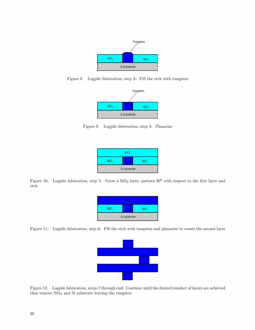
8. Logpile fabrication, step 3: Fill the etch with tungsten . . . . . . . . . . . . . . . . . . . . . . . . . . 21

9. Logpile fabrication, step 4: Planarize . . . . . . . . . . . . . . . . . . . . . . . . . . . . . . . . . . . . . . . . 21

10. Logpile fabrication, step 5: Grow a SiO2 layer, pattern 900 with respect to the firstlayer and etch . . . . . . . . . . . . . . . . . . . . . . . . . . . . . . . . . . . . . . . . . . . . . . . . . . . . . . . . . 21

11. Logpile fabrication, step 6: Fill the etch with tungsten and planarize to create thesecond layer . . . . . . . . . . . . . . . . . . . . . . . . . . . . . . . . . . . . . . . . . . . . . . . . . . . . . . . . . . . 21

12. Logpile fabrication, steps 7 through end: Continue until the desired number of layersare achieved then remove SiO2 and Si substrate leaving the tungsten . . . . . . . . . . . 22

13. Four logpile PGB patches covering a flat surface . . . . . . . . . . . . . . . . . . . . . . . . . . . . . . . . 22

14. Truncation of periodic structures . . . . . . . . . . . . . . . . . . . . . . . . . . . . . . . . . . . . . . . . . . . . 22

15. Seam formed by misalignment of two patches . . . . . . . . . . . . . . . . . . . . . . . . . . . . . . . . . . 23

16. Detail of misalignment . . . . . . . . . . . . . . . . . . . . . . . . . . . . . . . . . . . . . . . . . . . . . . . . . . . . . 23

8

17. Seam formed by a change in period . . . . . . . . . . . . . . . . . . . . . . . . . . . . . . . . . . . . . . . . . . 24

18. Overlap between two patches . . . . . . . . . . . . . . . . . . . . . . . . . . . . . . . . . . . . . . . . . . . . . . . . 24

19. Line defect . . . . . . . . . . . . . . . . . . . . . . . . . . . . . . . . . . . . . . . . . . . . . . . . . . . . . . . . . . . . . . . 25

20. Point defect . . . . . . . . . . . . . . . . . . . . . . . . . . . . . . . . . . . . . . . . . . . . . . . . . . . . . . . . . . . . . . 26

21. Periodic saw cuts introduced for thermal stability . . . . . . . . . . . . . . . . . . . . . . . . . . . . . . 26

22. Practical problem leading to seams and defects . . . . . . . . . . . . . . . . . . . . . . . . . . . . . . . . . 27

23. Definition of regions in truncation problems . . . . . . . . . . . . . . . . . . . . . . . . . . . . . . . . . . . 31

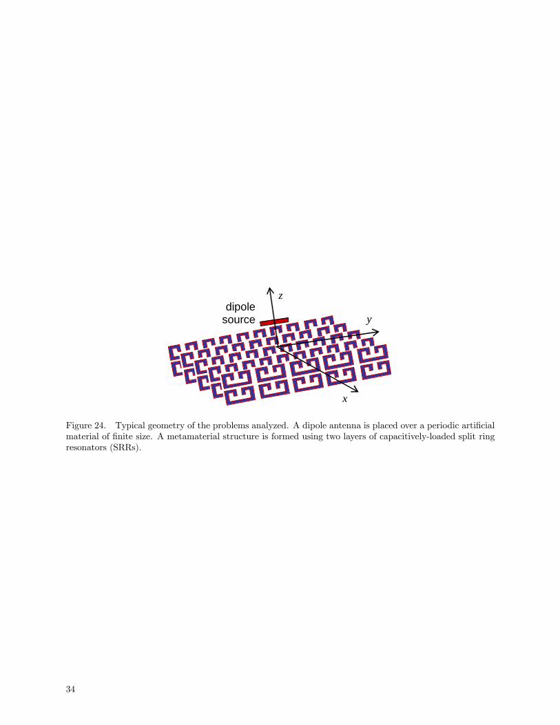
24. Typical geometry of the problems analyzed. A dipole antenna is placed over a periodicartificial material of finite size. A metamaterial structure is formed using twolayers of capacitively-loaded split ring resonators (SRRs). . . . . . . . . . . . . . . . . . . . . 34

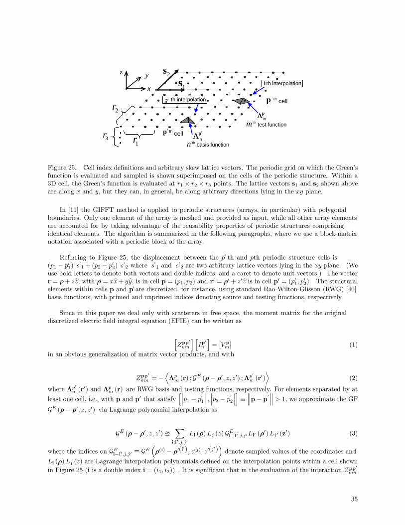
25. Cell index definitions and arbitrary skew lattice vectors. The periodic grid on whichthe Green’s function is evaluated and sampled is shown superimposed on the cellsof the periodic structure. Within a 3D cell, the Green’s function is evaluated atr1 × r2 × r3 points. The lattice vectors s1 and s2 shown above are along x and y, butthey can, in general, be along arbitrary directions lying in the xy plane. . . . . . . . . . 35

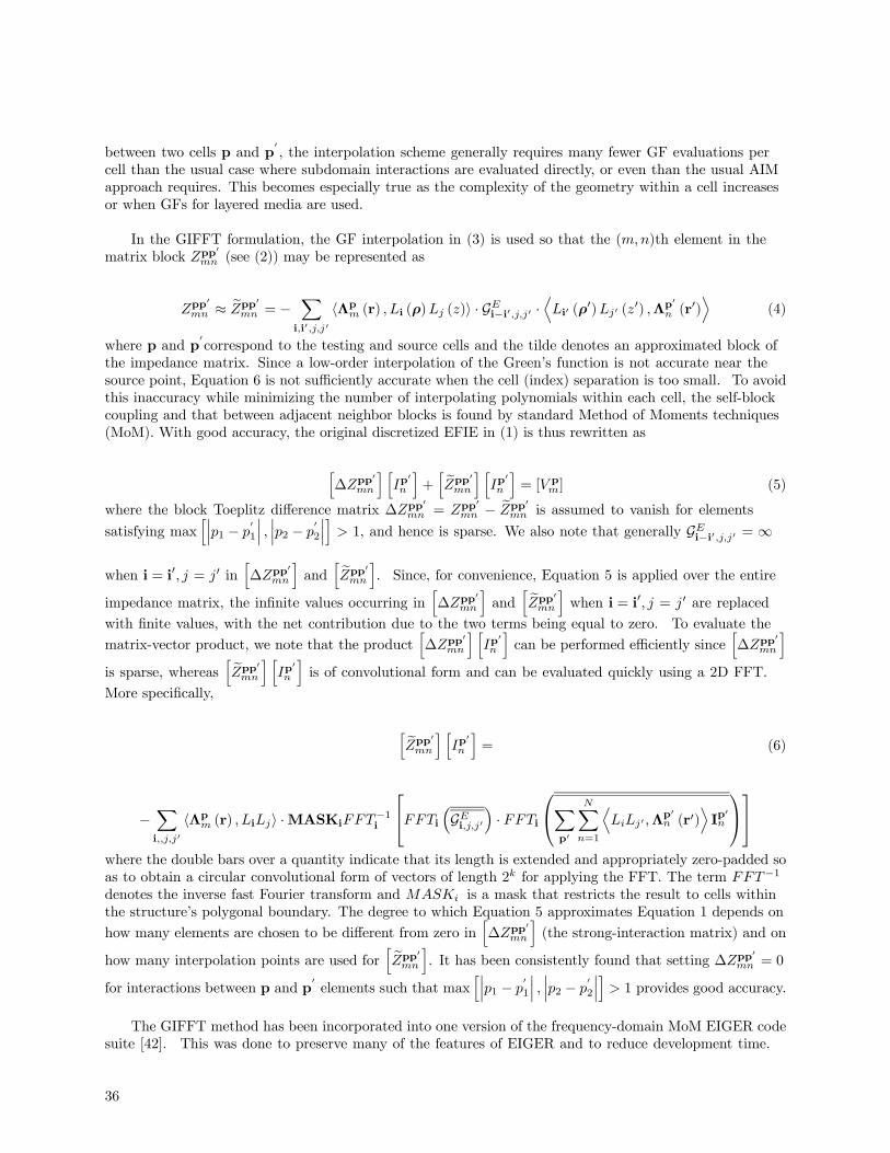
26. Periodic structure cells for a square lattice, with periods a and b that, for ametamaterial structure, are much smaller than the wavelength. The source islocated at the upper right corner of the mother cell p0 = (0, 0), and both exact andinterpolated GFs are evaluated in the cell p = (1, 1). The dots represent Green’sfunction sampling points over a cell cross section. . . . . . . . . . . . . . . . . . . . . . . . . . . . 37

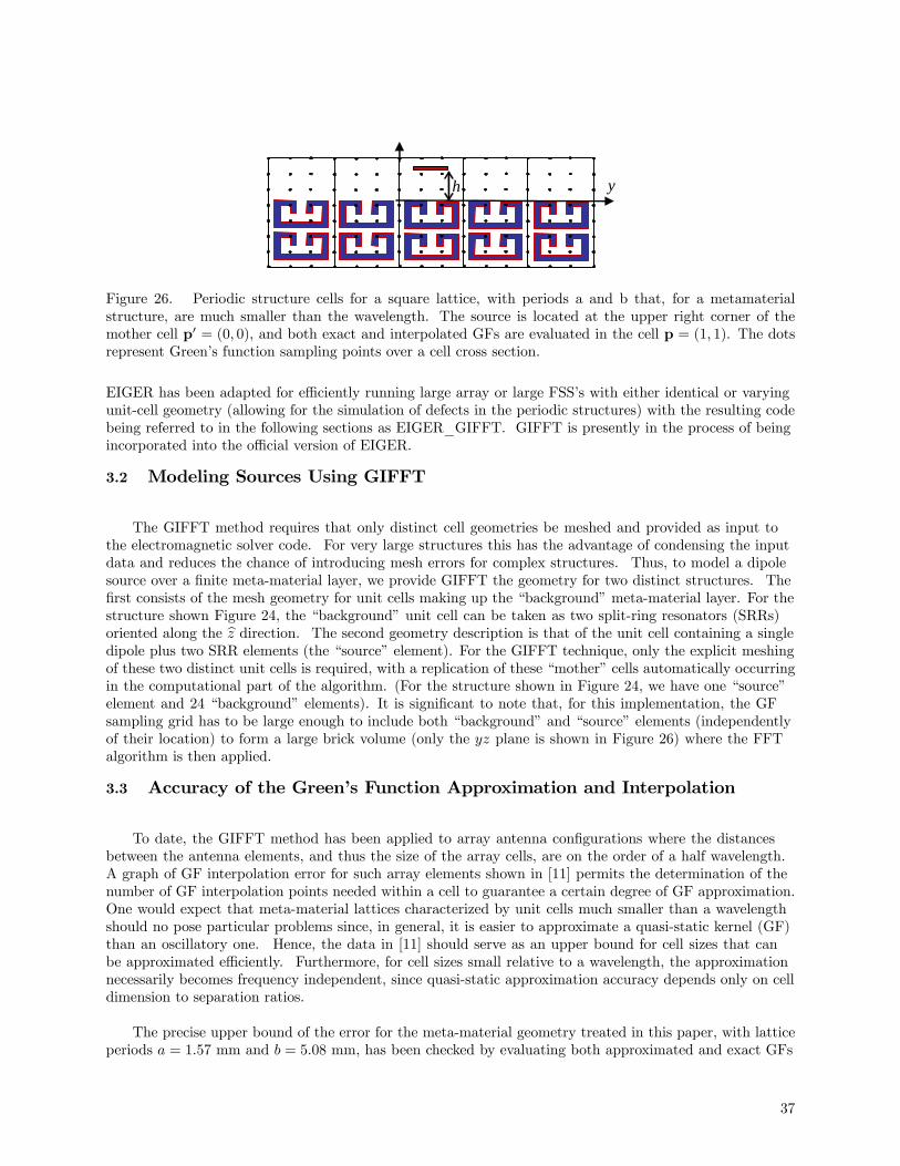
27. Periodic structure cells for a square lattice with periods a and b that, for ametamaterial structure, are much smaller than the wavelength. The source islocated at the upper right corner of the mother cell p0 = (0, 0) and both exact andinterpolated Green’s functions are evaluated in the cell p = (2, 1). . . . . . . . . . . . . . . 38

28. SRR geometry shown with dimensions and the associated mesh. . . . . . . . . . . . . . . . . . . 39

29. Results characterizing the reflection coefficient for a plane wave impinging frombroadside using two meshes with a varying number of quadrilaterals modeling theSRR thickness (see Figure 28). Mesh convergence is demonstrated at f = 15.7GHz, where the magnitude of the reflection coefficient is equal to unity and azero-crossing of the phase (at a reference plane) . . . . . . . . . . . . . . . . . . . . . . . . . . . . 40

9

30. A comparison of the average current densities over each unit cell (including both thetop and bottom SRRs) of a 9× 7 SRR metamaterial block using a Toeplitz MoMmethod and the GIFFT technique, at a frequency f = 13.8 GHz. . . . . . . . . . . . . . . . 41

31. Input impedance for a short dipole above a metamaterial made of 7× 3 periodic cells(two SRR in each cell). Two GF sampling grids have been used: 3 × 7× 7, and4 × 8 × 9, that provide the same results. A comparison with a standard MoMsolution in the frequency range from 12.9 GHz to 13.9 GHz is used to validate theGIFFT method. . . . . . . . . . . . . . . . . . . . . . . . . . . . . . . . . . . . . . . . . . . . . . . . . . . . . . . . 42

32. Input impedance of a dipole for various heights h ranging from 1.5 mm to 3 mm,for a small material made of 7 × 3 periodic cells. The location of the peaks isindependent of h showing behavior that is expected of the structure. The inputreactance remains largely capacitive due to the short length of the dipole. . . . . . . . 43

33. Input impedance for a short dipole located h = 2.5 mm above a metamaterial substratemade of 7× 3 and 33× 11 cells (two SRRs in each cell). Also, the input impedancefor a dipole with h = 2 mm is shown. . . . . . . . . . . . . . . . . . . . . . . . . . . . . . . . . . . . . . . 43

34. Radiation pattern of a dipole at a height h = 2.5 mm, for the small (7× 3 cells) and thelarge (33× 11 cells) metamaterial substrate, at frequency f = 13.73 GHz. . . . . . . . . . 44

35. Radiation pattern for various frequencies of a dipole located at h = 2.5 mm above alarge (33× 11 cells) metamaterial substrate. . . . . . . . . . . . . . . . . . . . . . . . . . . . . . . . . 44

36. Unit-cell geometry used to form a planar, PEC, strip-dipole array at z = 0. . . . . . . . . 45

37. The element numbering scheme for an example 3× 3 array. . . . . . . . . . . . . . . . . . . . . . . . 46

38. Current distributions for select elements of a 5× 5 array. . . . . . . . . . . . . . . . . . . . . . . . . 47

39. Current distributions for select elements of a 10× 10 array. . . . . . . . . . . . . . . . . . . . . . . . 48

40. Contour plot of the current magnitude for an infinite array of the strip dipole shownin Figure 36. . . . . . . . . . . . . . . . . . . . . . . . . . . . . . . . . . . . . . . . . . . . . . . . . . . . . . . . . . 48

41. Contour plot of the current magnitude for a 10× 10 array of the strip dipole shown inFigure 36. . . . . . . . . . . . . . . . . . . . . . . . . . . . . . . . . . . . . . . . . . . . . . . . . . . . . . . . . . . . 49

42. Current distributions for select elements of a 40× 40 array. . . . . . . . . . . . . . . . . . . . . . . . 50

10

43. Effect on the current density of a 450 rotation of the center element of a 5 × 5 stripdipole array . . . . . . . . . . . . . . . . . . . . . . . . . . . . . . . . . . . . . . . . . . . . . . . . . . . . . . . . . . . 52

44. Effect on Eθ of a 450 rotation of the center element of a 5× 5 strip dipole array . . . . . . 53

45. Effect on Eφ of a 450 rotation of the center element of a 5× 5 strip dipole array . . . . . . 54

46. General seam geometry . . . . . . . . . . . . . . . . . . . . . . . . . . . . . . . . . . . . . . . . . . . . . . . . . . . . 55

47. Geometry of a 1d seam . . . . . . . . . . . . . . . . . . . . . . . . . . . . . . . . . . . . . . . . . . . . . . . . . . . . . 57

48. Finite seam . . . . . . . . . . . . . . . . . . . . . . . . . . . . . . . . . . . . . . . . . . . . . . . . . . . . . . . . . . . . . . 57

49. Current on strip at the m=0 position . . . . . . . . . . . . . . . . . . . . . . . . . . . . . . . . . . . . . . . . . 58

50. Current on strip at the m=-1 position . . . . . . . . . . . . . . . . . . . . . . . . . . . . . . . . . . . . . . . . 59

51. Current on strip at the m=+1 position . . . . . . . . . . . . . . . . . . . . . . . . . . . . . . . . . . . . . . . 59

52. Current on strip at the m=+2 position . . . . . . . . . . . . . . . . . . . . . . . . . . . . . . . . . . . . . . . 60

53. Current on strip at the m=-2 position . . . . . . . . . . . . . . . . . . . . . . . . . . . . . . . . . . . . . . . . 60

54. Basis function for the difference current (Jd) . . . . . . . . . . . . . . . . . . . . . . . . . . . . . . . . . . . 61

55. Basis function for the known periodic current . . . . . . . . . . . . . . . . . . . . . . . . . . . . . . . . . . 62

56. Current near a 1d seam . . . . . . . . . . . . . . . . . . . . . . . . . . . . . . . . . . . . . . . . . . . . . . . . . . . . 62

57. Detail of two-dimensional seam geometry . . . . . . . . . . . . . . . . . . . . . . . . . . . . . . . . . . . . . 63

58. Physical configuration and coordinates for a planar periodic array of point sourceswith interelement spacing d along z. Rn is the distance between observation pointr ≡ (ρ, z) and the nth source element r0n ≡ (0, nd). . . . . . . . . . . . . . . . . . . . . . . . . . . . . . 66

59. Path of integration. Expressing k = |k| exp(jφk) (Im k ≤ 0, thus φk < 0), ands = |s| exp(jφs), the region of convergence of (15) is given in (16) and (17). . . . . . . . . 66

11

60. Convergence of the Ewald sums in (18) with (28) and (33) evaluated at threeobservation points with ρ = 0.0, 0.01d, 0.1d and z = 0.1d. Percentage relative errorversus number of terms N (Q = N) in the sums for two cases with period d = 0.05λand d = 0.5λ. Curves for ρ = 0 and ρ = 0.01d are superimposed. . . . . . . . . . . . . . . . . . 72

61. Convergence of the two individual series Gspectral and Gspatial in (28) and (33) forvarious choices of the splitting Ewald parameter E. . . . . . . . . . . . . . . . . . . . . . . . . . . 73

62. Convergence versus the number of terms P of p-sum in (28) for observation pointsranging from ρ = 0.01d to 0.2d. The period is d = 0.5λ. (a) percentage relative error(44) of the spectral sum (28) where the reference solution is still evaluated using(28) with P = 60. (b) percentage relative error (43) of the Green’s function G in(18) with (12) as reference solution. . . . . . . . . . . . . . . . . . . . . . . . . . . . . . . . . . . . . . . . 74

63. High frequency case (period larger than the wavelength: here, d = 5.5λ.) (a) Percentagerelative error (43) versus number of terms N (Q = 4N). (b) Convergence rates forindividual series Gspectral and Gspatial, in (28) and (33), respectively. One term(n = 0) in Gspatial is sufficient for excellent accuracy. In this case the choice of theoptimum parameter E = E0 would cause numerical errors, as explained in Section4.2.7. Three different choices of the E parameters are analyzed here. Increasingthe ratio E/E0 results in a larger number of terms in Gspectral to reach convergence.A smaller ratio E/E0 would decrease the number of necessary terms in Gspectral butwould result in a loss of accuracy. . . . . . . . . . . . . . . . . . . . . . . . . . . . . . . . . . . . . . . . . . 75

64. FSS illuminated by a plane wave or by a beam source . . . . . . . . . . . . . . . . . . . . . . . . . . . 81

65. Two equivalent problems from a phenomenological point of view . . . . . . . . . . . . . . . . . . 82

66. A plane wave impinging on a flat FSS generates a reflected field and diffracted fieldsfrom the edges and corners of the FSS at the observation point P. . . . . . . . . . . . . . 83

67. The three wave species, the reflected field, the edge diffracted field, and corner (orvertex) diffracted field arriving at the observation point P. Also shown are the twocanonical problems that can be used to determine the mathematical form of theseray contributions. . . . . . . . . . . . . . . . . . . . . . . . . . . . . . . . . . . . . . . . . . . . . . . . . . . . . . . 83

68. The three wave species that are to be multiplied by the radiation pattern of theelementary array element. The approximation described in the text (the POapproximation) results by assuming that all the element radiation patterns arealike. . . . . . . . . . . . . . . . . . . . . . . . . . . . . . . . . . . . . . . . . . . . . . . . . . . . . . . . . . . . . . . . . 84

69. A seam between two frequency-selective-surfaces. Besides the standard reflected andtransmitted field contributions associated with the FSS, three rays originate fromthe seam: one edge-like diffracted field and two vertex-like diffracted fields. . . . . . 86

12

70. The far-field E-plane radiation pattern produced by the 50× 50 dipole array. . . . . . . . . 87

71. Direction of the observation scan used to highlight the edge-diffracted fields. . . . . . . . . 88

72. Diffracted field along the observation scan shown in Figure 71. . . . . . . . . . . . . . . . . . . . . 88

73. Fit of the diffracted field, along the observation scan of Figure 71, with the curve∝ 1/√ρ . . . . . . . . . . . . . . . . . . . . . . . . . . . . . . . . . . . . . . . . . . . . . . . . . . . . . . . . . . . . . . . 89

74. A seam created by a junction between two periodic structures. . . . . . . . . . . . . . . . . . . . 90

75. The far-field E-plane radiation patterns produced by a vertical seam in a 50 × 50array . . . . . . . . . . . . . . . . . . . . . . . . . . . . . . . . . . . . . . . . . . . . . . . . . . . . . . . . . . . . . . . . 90

13

Tables

A Array input file for a 5X5 array of identical strip elements. . . . . . . . . . . . . . . . . . . . . . . . 46

B Matrix fill and solve times for a 5× 5 and 10× 10 element array using GIFFT and thestandard MoM. . . . . . . . . . . . . . . . . . . . . . . . . . . . . . . . . . . . . . . . . . . . . . . . . . . . . . . . . 51

C Array input file for a 5X5 array with center defect element. . . . . . . . . . . . . . . . . . . . . . . 56

14

Analysis of Electromagnetic Scattering byNearly Periodic Structures: An LDRD Report

1 Introduction

The goal of this LDRD is to provide the critical computational analysis and design tools for developingthe “science” of how Photonic Band Gap (PBG) structures operate so that they can be fielded withoutresorting to excessive experimental prototyping. Interest in PBG structures has increased in recent yearsbecause they have the ability to manipulate light in the optical and infrared wavelength ranges. Byintentionally introducing defects in a PBG structure, the optical band gap can be modified, which leadsto the possibility of new optical devices. In the remainder of this introduction we will describe thecharacteristics of a PBG structure, how one is built and some of its applications. We will compare andcontrast PBG structures to periodic structures that are common in the microwave domain. We will definesome terms useful in describing periodicity and apply these terms to describe some actual PBG structures.Finally, we will describe in detail what this LDRD is about.

1.1 Description of a PBG Structure

A PBG structure is a material that inhibits photon propagation over a narrow band of frequenciesregardless of the direction of the propagation. This band of frequencies, borrowing from the terminology ofsemi-conductors, is known as the “band gap” or “forbidden band”. Photons with frequencies outside theband gap propagate through the PBG without attenuation.

The PBG structure is made by periodically changing the material’s index of refraction as a functionof location. Initially this was done in the microwave regime by simply drilling regularly-spaced holesthrough a slab of dielectric material. Typically, the period of the PBG structure is on the order of thewavelength associated with the band gap center frequency [1]. An electromagnetic wave with a frequencyin the band gap is partially reflected from each change in the index of refraction. The reflected wavesadd constructively, while the transmitted waves adds destructively causing the total wave to attenuateas it propagates through the material. Waves with a frequency out of the band gap are reflected andtransmitted out of phase with each other and do not attenuate. The difficulty is to get this interference tooccur irrespective of propagation direction. The solution thus far is to modulate the index of refraction inthree dimensions based on the face-center-cubic crystalline structure found in diamond [2].

PBG applications include optical fibers where a PBG material surrounds an inner core. In contrast toconventional optical fibers, where the core has a high refractive index to confine the light by total internalreflection, the PBG material allows the core to be a low index of refraction — even a void — which allowsmore power and information to be passed through the fiber. In the area of light-emitting diodes, a PBGstructure can extract light from the diode with greater than 50% efficiency. Titanium dioxide particlessmaller than a micron can self-assemble into a PBG structure. Ordinarily, titanium dioxide is a whitepigment used in paint and in making white paper. The PBG structure scatters light coherently andimparts more whiteness for less mass of titanium dioxide. Introducing a defect in a PBG structure trapslight and forms a type of electromagnetic cavity. This small cavity can be used to build small nano-scalelasers. Finally, PBG structures also occur in nature in butterfly wings and opals [1].

Microwave engineering also has periodic structures that exhibit band gap behavior. One such structureis known as a frequency selective surface (FSS) [3]. FSS’s are used as microwave filters, in radomes and asfrequency dependent reflectors for space re-use in reflector antenna systems [4]. In the infrared, FSS’s are

15

used as polarizers, beam splitters and mirrors [5]. It is useful to compare and contrast the PBG and FSSto see if they have any problems in common, and given that they do, if any analysis techniques from onediscipline can be applied to the other. As the name implies, the FSS is a surface, usually made of thin,metallic patches (a large modulation of index of refraction) placed periodically on a thin sheet of dielectric.PBG structures, on the other hand, are inherently three-dimensional because of the requirement to have aband gap irrespective of propagation direction. In practice, however, this distinction blurs since, on theone hand, the PBG structure is usually truncated in one of its dimensions to make a slab and on the otherhand, several FSS’s can be stacked to engineer certain band characteristics, which give it some thickness[6]. Initially, PBG structures were made of dielectric material (or by the removal of dielectric material) tocut down on loss, but this also is not a distinguishing feature since in order to ease fabrication and reducesize, PBG structures are now also being made of metal [5]. Indeed, some of the PBG’s fabricated at Sandiaare made of tungsten. The main difference between FSS’s and PBG structures is that the PBG has amore stringent requirement to be independent of propagation direction. In a reflector antenna application,the FSS may have a bandgap that varies as a function of incident angle, but the surface is placed at aposition where the band gap requirements are satisfied. If the FSS is being used in a stealth application,where the incident angle has a greater variation, the FSS must have a more stringent bandgap versus anglerequirement, more like a PBG.

PBG structures were initially studied by optical and solid-state physicists, so from an analysis point ofview they are approached as optical semiconductors [2], [7], [8]. Even the language of the analysis is thatof semi-conductors — so in the first PBG structure, which was created by drilling holes through a dielectricslab, filling the intersection of the holes with a dielectric was referred to as adding a donor defect and slicingthrough the dielectric between holes was referred to as adding an acceptor defect. In the microwave realm,the periodic structure is viewed as a scatterer of electromagnetic waves. Once the language difficultiesare overcome, the analysis techniques are similar to one another in that both are geared toward structureshaving periods that are approximately equal to a wavelength, albeit wavelengths that are vastly different insize. Until recently, however, the two disciplines seemed to be unaware of each other. In this LDRD wewill apply techniques that have been developed in the microwave regime to problems arising in the PBGstructures. The tiny wavelength in the PBG regime, however, leads to problems that arise solely becauseof required tight manufacturing tolerances. These problems don’t occur in the microwave world because ofits larger wavelength and therefore, haven’t been a subject of microwave research. Details will be discussedlater.

In order to define some useful terms, Figure 1 shows a portion of a periodic structure, typical of an FSS.We are viewing the FSS looking down the bz axis. The unit cell, which takes the form of a parallelogram, isreplicated along the lattice vectors bS1 and bS2 an infinite number of times tiling the entire z = 0 surface.Along bS1 the unit cells are replicated with a period a. Along bS2 they are replicated with a period b. Figure2 shows a plane wave illumination of the periodic structure. The plane wave is represented by the wavevector

−→k , which is defined in terms of the spherical coordinates θ and φ as shown. The sets of three black

dots at each edge of the periodic structure indicate that it is actually infinite in extent. Although theseterms are commonly used to define an infinite structure, they can also be used to describe nearly-periodicsurfaces. For example, if the periodic structure were truncated to a finite area, the unit cell could bereplicated a finite number of times along the lattice vectors to cover the array. If a defect or seam ispresent, replicating the unit cell could describe the quasi-periodic area around the defect or seam.

1.2 Examples of PBG Structures

Typical PBG structures are many layers thick, as shown in Figures 3, 4 and 5. The wavelength rangeof interest for all these structures is between 3 and 15 μm. Figure 3 shows a PBG made by Sandia NationalLaboratories that consists of five layers of long, square tungsten rods. The cross-section of each rod is 1.2μm by 1.2 μm and the rods are all approximately 1 cm long. The period of a single layer is 4.2 μm. Each

16

S1

S2

UnitCell

a

b

Figure 1. Definition of the unit cell and periodic lattice

layer is rotated 900 with respect to its neighboring layers. If we number the layers starting with layer oneon the bottom and layer five at the top, layers one and five are identical to each other. Layer three hasrods that are in the same direction as layer one, but offset laterally by one half a period. Layers two andfour are rotated 900 with respect to layer one with layer four offset laterally from layer two by one half aperiod. This type of PBG is called a logpile. The logpile can be described using the infinite periodic slabparameters defined in Figure 1 as bS1 = bx, bS2 = by, a = b = 4.2 μm. Note that the unit cell of the logpile isfive layers thick and current continuity must be enforced across neighboring unit cells and between layers.

Figure 4 shows another example of a PBG structure — this one made of rings stacked upon each other.The rings are 4.3 μm in diameter with walls that are 0.75 μm thick. The periodic slab parameters in thiscase are bS1 = bx, bS2 = by, a = b = 5 μm. Figure 5 shows a PBG structure with a “Y” shape stacked uponeach other to form the unit cell.

Figures 6 through 12 show the steps needed to fabricate a logpile. The first step, as shown in Figure 6,is to deposit a 1.2 μm layer of SiO2 on a Si substrate. The SiO2 layer is periodically etched down to the Sisubstrate with grooves that are 1.2 μm wide and spaced 4.2 μm away from each other. A single examplegroove is shown in Figure 7. The third step is to fill all the grooves with tungsten, as shown in Figure 8.The tungsten protrudes above the SiO2 layer presenting a rough top. Figure 9 shows that the protrudingpart of the tungsten is ground down to the surface of the SiO2 layer in a chemical-mechanical polishingprocess known as “planarizing”. This last step is essential because it creates a flat surface that serves asa base for building the next layer. These first four steps create the first layer of logs. The next layer oflogs is made by repeating the first four steps, but etching grooves in a direction 900 with respect to thefirst layer. This is shown in Figures 10 and 11. This process continues for each layer until the requirednumber of layers are made. A final step, which is shown in Figure 12, removes the SiO2 portions and theSi substrate leaving behind the finished tungsten logpile.

17

x

y

z

S1

S2

k

θ

Periodic Surface

φ

Figure 2. Oblique view of the periodic structure with an incident plane wave

Figure 3. Example of a PBG structure — a five layer logpile

18

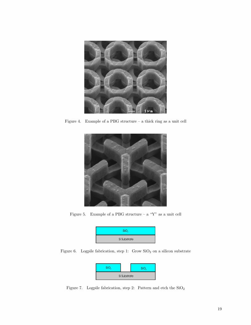
Figure 4. Example of a PBG structure — a thick ring as a unit cell

Figure 5. Example of a PBG structure — a “Y” as a unit cell

Si Substrate

Figure 6. Logpile fabrication, step 1: Grow SiO2 on a silicon substrate

Si Substrate

Figure 7. Logpile fabrication, step 2: Pattern and etch the SiO2

19

Si Substrate

Tungsten

Figure 8. Logpile fabrication, step 3: Fill the etch with tungsten

Si Substrate

Tungsten

Figure 9. Logpile fabrication, step 4: Planarize

Si Substrate

W

Figure 10. Logpile fabrication, step 5: Grow a SiO2 layer, pattern 900 with respect to the first layer andetch

Si Substrate

W

W

Figure 11. Logpile fabrication, step 6: Fill the etch with tungsten and planarize to create the second layer

W

Figure 12. Logpile fabrication, steps 7 through end: Continue until the desired number of layers are achievedthen remove SiO2 and Si substrate leaving the tungsten

20

1.3 Scope of Work

The characteristics of a PBG structure, such as bandgap frequency, can be engineered by varying thelattice periodicity and by varying the design of the unit cell. We see from the photographs of actual PBGstructures (Figures 3 - 5) that on the scale of a few unit cells, manufacturing techniques are sophisticatedenough that the PBG structures are in fact locally periodic. By assuming periodicity, we can analyze theperformance of a PBG illuminated by a plane wave by invoking the fact that the fields are identical fromunit cell to unit cell except for a phase shift dictated by the angle of incidence of the plane wave and thedistance between unit cells. If the plane wave were normally incident on the structure (incident alongbz), for example, there would be no phase shift at all and the fields would be identical over each unit cell.In a numerical solution, this fact allows us to devote our unknowns to modeling a single unit cell ratherthan the entire structure. Generally, if we invoke periodicity on a sub-wavelength sized unit cell and useapproximately 10 unknowns per wavelength, we can limit the number of unknowns required to model theproblem to less than 100.

In reality, however, the structure is never infinite in extent so the assumption of periodicity is alwaysan approximation. Analyzing the effect that truncation has on the infinite structure is of concern. ThePBG structure of interest is limited by manufacturing constraints to be a square patch roughly 1 cm by1 cm (1000 by 1000 wavelengths if the wavelength is 10 μm). We can put patches together to cover alarge object, but because the patches are physically so small this is difficult and leads to other departuresfrom periodicity. Figure 13, which shows four square patch PBG’s placed on a flat object, will be usedto demonstrate what can happen due to poor placement. We see that the perimeter of the four patchesis a straight-forward example of truncation. This type of truncation also occurs in the microwave regimebecause phased arrays and FSS’s are also of finite extent. Extensive work has been done by the microwavecommunity to analyze this type of truncation. Gaps between the patches, which are physically small (onthe order of 100 microns), but large in terms of wavelengths, is also considered a truncation. This type oftruncation doesn’t occur in the microwave regime because the unit cells are physically large enough thatgaps can be eliminated. Figure 14 shows the problem of truncation in greater detail.

If two neighboring patches are brought to within a half a wavelength of each other, they can form aseam. In general, a seam occurs when the characteristics of the unit cell — size, contents or both — changefrom one region to another. If two identical patches are carefully butted against each other so that the unitcells align, the periodicity is maintained and no seam is formed. If, however, the two identical patches aremisaligned, as shown in Figure 15, a seam is formed. The size of the unit cell is the same in both patches,but the shift can be thought of as changing the contents of the unit cell from one side of the seam to theother as shown in Figure 16. Figure 17 shows a seam formed when the size of the unit cell changes thuschanging the periodic spacing. If the two patches are brought close enough together, they can overlap asshown in Figure 18. In the microwave regime seams have not been studied at all because the wavelength islarge enough that the unit cells can be manufactured identically and are easily aligned to a sub-wavelengthtolerance.

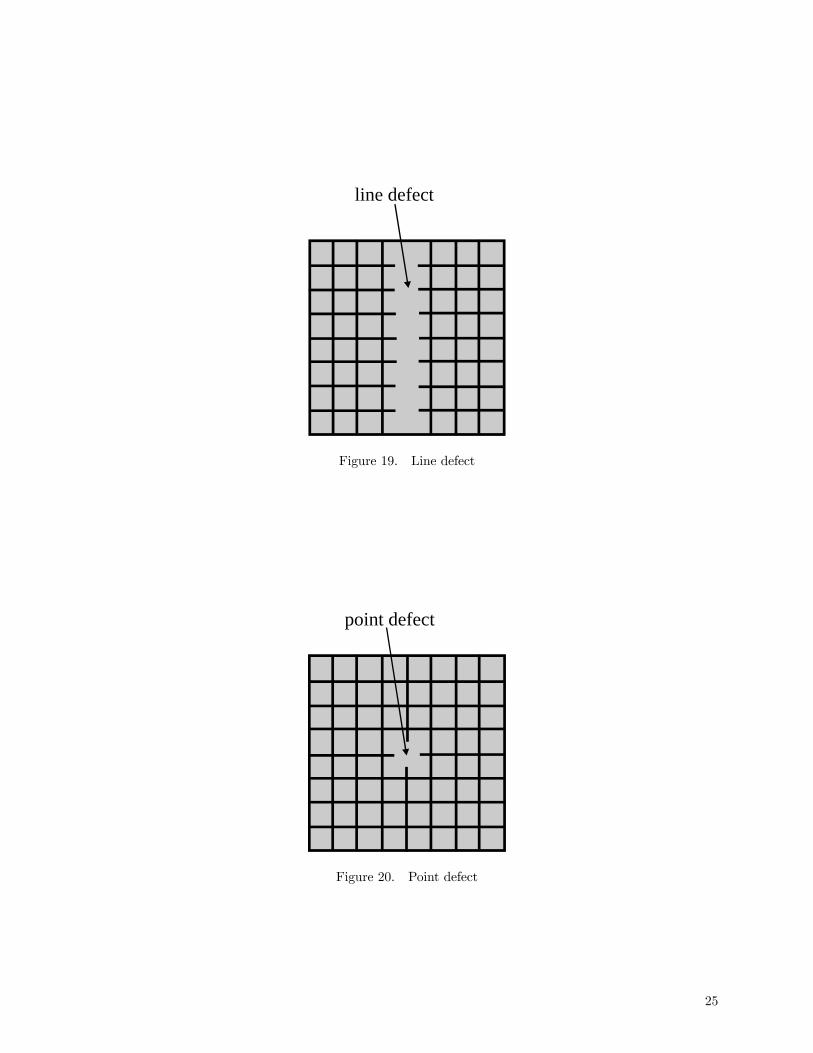
Within the PBG patch itself, since the unit cells are physically small, unintentional defects can occur inthe lattice due to manufacturing mistakes, again breaking the periodicity. Defects can also be introducedintentionally to modify the scattering characteristics of the PBG structure. If defects are introduced alonga line, as shown in Figure 19, this is known as a line defect, while a single, isolated defect, as shown inFigure 20 is known as a point defect [9]. Defects can also be introduced for mechanical reasons. Forexample, if the logpile is made of two different materials each with its own coefficient of thermal expansion,the patch has the potential to bend and de-laminate due to thermally induced stress. One solution to thisproblem is to introduce periodic cuts in the bars to relieve the stress as shown Figure 21.

Maintaining periodicity becomes even more difficult when the PBG patches are applied to a non-planar

21

Figure 13. Four logpile PGB patches covering a flat surface

truncation (100 m ~ 10 μ λ)

conventional truncation

Figure 14. Truncation of periodic structures

22

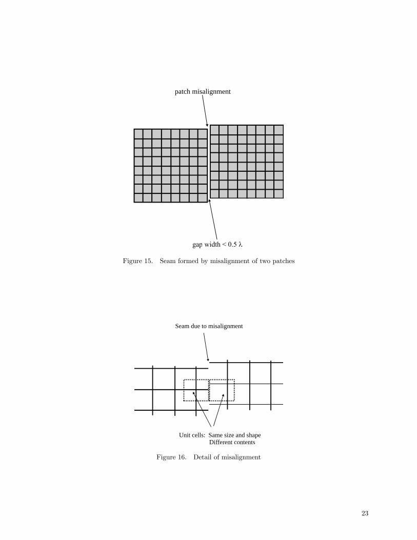
patch misalignment

Figure 15. Seam formed by misalignment of two patches

Seam due to misalignment

Unit cells: Same size and shape Different contents

Figure 16. Detail of misalignment

23

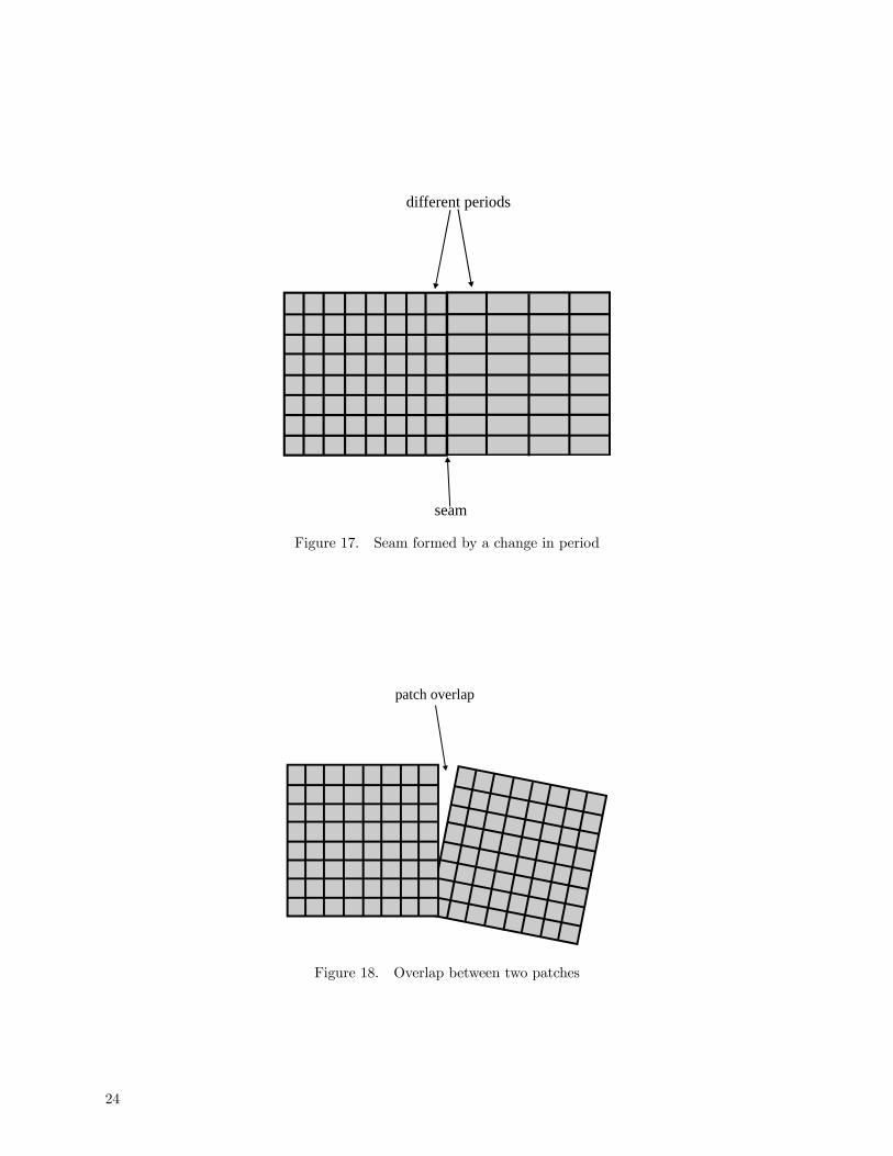
different periods

seam

Figure 17. Seam formed by a change in period

patch overlap

Figure 18. Overlap between two patches

24

line defect

Figure 19. Line defect

point defect

Figure 20. Point defect

25

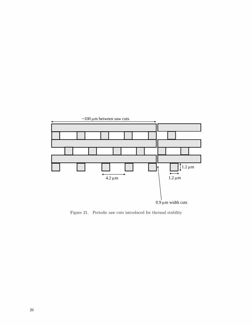
~100 m between saw cutsμ

1.2 mμ

1.2 mμ

0.9 m width cutsμ

4.2 mμ

Figure 21. Periodic saw cuts introduced for thermal stability

26

Object

non-planarwrap

truncation

defect

periodicitychange (seam)

PBG patches

Figure 22. Practical problem leading to seams and defects

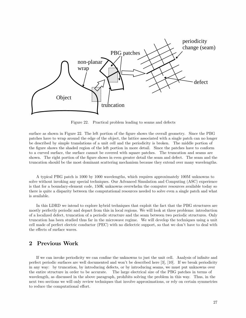
surface as shown in Figure 22. The left portion of the figure shows the overall geometry. Since the PBGpatches have to wrap around the edge of the object, the lattice associated with a single patch can no longerbe described by simple translations of a unit cell and the periodicity is broken. The middle portion ofthe figure shows the shaded region of the left portion in more detail. Since the patches have to conformto a curved surface, the surface cannot be covered with square patches. The truncation and seams areshown. The right portion of the figure shows in even greater detail the seam and defect. The seam and thetruncation should be the most dominant scattering mechanism because they extend over many wavelengths.

A typical PBG patch is 1000 by 1000 wavelengths, which requires approximately 100M unknowns tosolve without invoking any special techniques. Our Advanced Simulation and Computing (ASC) experienceis that for a boundary-element code, 150K unknowns overwhelm the computer resources available today sothere is quite a disparity between the computational resources needed to solve even a single patch and whatis available.

In this LDRD we intend to explore hybrid techniques that exploit the fact that the PBG structures aremostly perfectly periodic and depart from this in local regions. We will look at three problems: introductionof a localized defect, truncation of a periodic structure and the seam between two periodic structures. Onlytruncation has been studied thus far in the microwave regime. We will develop the techniques using a unitcell made of perfect electric conductor (PEC) with no dielectric support, so that we don’t have to deal withthe effects of surface waves.

2 Previous Work

If we can invoke periodicity we can confine the unknowns to just the unit cell. Analysis of infinite andperfect periodic surfaces are well documented and won’t be described here [3], [10]. If we break periodicityin any way: by truncation, by introducing defects, or by introducing seams, we must put unknowns overthe entire structure in order to be accurate. The large electrical size of the PBG patches in terms ofwavelength, as discussed in the above paragraph, prohibits solving the problem in this way. Thus, in thenext two sections we will only review techniques that involve approximations, or rely on certain symmetriesto reduce the computational effort.

27

2.1 Work Pertaining to Defects

Defects are important in PBG structures because they can introduce a small band of frequencies withinthe forbidden band across which the attenuation is reduced. Defects are purposefully introduced eitherby cutting a gap in the walls between a single pair of array holes drilled in a dielectric slab (an acceptordefect), or by placing a dielectric sphere in one of the array holes (a donor defect) [7]. These single-pointdefects are analyzed by introducing a so-called super cell where a unit cell with a defect is surroundedby unit cells without defects [9]. The entire conglomeration of unit cells is essentially treated as a newunit cell with periodic boundary conditions imposed on its exposed faces. The result is that a new periodis substituted for the old. A new super cell made of eight original cells, for example, would double theoriginal period putting a defect every other unit cell.

Although the introduction of periodic defects may be necessary to cause the desired bandgapmodifications, for this project we are interested in analyzing a true single-point defect where no newperiodic cell is invoked. We will do this by modifying a technique developed by Fasenfest, which wasoriginally used to study truncation effects of phased arrays [11]. Fasenfest’s technique, the Green’s FunctionInterpolation with a Fast Fourier Transform (GIFFT), depends on the fact that the elements of the phasedarray, although truncated, conform to a periodic lattice. In other words, the spacing a and b in Figure1 can not change over the array. The main features of GIFFT are that interactions between sufficientlyseparated array elements are performed using a relatively coarse interpolation of the Green’s function ona uniform grid commensurate with the array’s periodicity — thus the need for a fixed periodicity. TheGreen’s function is approximated on the interpolated grid as a sum of separable functions (functions whichare a product of a function of the source coordinates and a function of the observation coordinates) which,together with the periodic nature of the array, allows for only near interactions to be computed explicitlyand thus lead to an efficient matrix fill. The interpolatory coefficients (representing sampled values of theGreen’s function) are of convolutional form and therefore an FFT can be used to efficiently calculate thematrix-vector product when using an iterative solver.

2.2 Work Pertaining to Seams

Seams, although potentially important, have not yet been studied in the PBG community. Aspreviously discussed, seams really don’t occur in microwave devices so they also haven’t been studied bythe microwave community. The microwave problem closest to the seam problem is that of truncation. Tostudy both truncation and curvature problems, Cwik reduces the number of unknowns required to grid theentire surface by studying a two-dimensional problem — scattering from a finite array of strips — and notestwo approximations that could point the way to solving the three-dimensional problem [14]. For a curvedgeometry he treats each strip as if it were a member of an infinite, planar, periodic surface with a normalcoinciding with the normal of the strip. This approximation accounts for the curvature of the structure,but not for its truncation. The second approximation solves for the currents on strips near the array edgefor a small problem and uses these edge currents to replace the edge currents in a larger problem. Koextends Cwik’s work to three dimensions by looking at an FSS that is periodic and infinite in one directionand periodic, but truncated in the other direction [15]. Like Cwik, Ko notes that the surface currents arealmost identical for all the patches in the array except near the edge and postulates using the currentsfrom the infinite periodic surface for the interior currents of the truncated surface and solving only for thecurrents near the edge. Based on these results, attempts were made to use the solution of the infinite,periodic structure in the center region of a finite FSS and to put subdomain unknowns only on the edgeregion. Difficulty arises from matching the two solutions at the boundary between the center and edgeregion and how one chooses the location of that boundary [16].

Philips [17] analyzes an FSS embedded in a paraboloidal, dielectric radome. He uses a ray-tracing

28

method to do the analysis similar to the method known as “Shooting and Bouncing Rays” (SBR) wherea number of rays are launched at the mouth of an open cavity, such as a engine inlet, and the rays areindividually followed as they bounce throughout the cavity to an output plane [18]. For Philips’ case,whenever the ray encounters the curved wall of the radome, the dielectric and the FSS are treated as locallyplanar and infinite. The rays are traced as they propagate through the dielectric and encounter the FSSmultiple times. The rays are tracked in the dielectric slab until they emerge from the other side or decayto where they can be ignored. By separating the FSS interaction from those of the dielectric slab, thecurvature is allowed to change for each bounce and the curvature is accounted for more accurately thantreating the slab and the FSS as a single unit. Since Philips only accounts for the FSS using a reflectionand transmission coefficient for the specular ray (zeroth order Floquet mode) the boundary conditionsare only enforced approximately. This paper shows that high-frequency ray techniques can be used forscattering type problems involving FSS’s. Since each ray interacts with an infinite structure, no truncationeffects are taken into account.

A large number of papers study truncated FSS’s by assuming that the current distribution on each unitcell is the same as that of the infinite FSS weighted by an assumed distribution across the truncated FSS.For example, if the weighting is uniform, the current next to the edge of the truncated FSS is identicalto the current in the center of the FSS. By making this approximation, the papers bypass the majorcomputational work of the problem and are left with the much easier problem of finding the field due tothe known currents. Additionally, they are free to use various approximations to simplify this task evenfurther. We will next discuss some of the papers that use this technique.

Rahmat-Samii examines a dual-reflector antenna system which has as one of its components adoubly-curved and finite FSS subreflector. He uses the same approach as Cwik [14], but on a much morecomplicated problem [4]. At various points around the curved surface, he first finds the local tangent planeand then calculates the reflection and transmission coefficients of an infinite periodic FSS coincident withthat plane. The reflection and transmission coefficients account for the fact that the incident wave fromthe feed changes orientation with respect to the FSS at different points of the curved surface, but it doesnot account for the fact that the current on an element near the edge of the FSS will be different from thecurrent on an element near the middle of the FSS due to the presence of the edge. From the reflection andtransmission coefficients, Rahmat-Samii finds equivalent currents on a Huygens surface surrounding theFSS and allows the fields due to the currents to radiate toward the main reflector. This step effectivelytruncates the current and accounts somewhat for the finiteness of the FSS. If this technique were appliedto a flat, finite FSS, for example, it would consist of finding the current on a unit cell of a single, infiniteFSS and then having this current exist on the unit cells making up the original FSS. The finiteness doesn’taffect the current distribution, but does affect the field due to the currents.

Ishimaru solves for the active impedance of a finite array of dipole elements with progressive phasingby assuming that the current on each array element is identical except for a weighting coefficient [19]. Thecurrent on the elements are weighted by an aperture distribution function across the entire array. Throughuse of the Poisson Summation formula, which converts a spatial sum to a sum of Fourier transforms, andusing a spatial Fourier transform to represent the impedance in terms of the impedance of an infinite array,the active impedance is expressed as a convolution between the impedance of the infinite periodic structureand the Fourier transform of the aperture distribution. The aperture distribution can theoretically be anyfunction, but the examples all use a uniform distribution. The convolution integral is sampled at a pointdictated by the element-to-element phasing.

Carin looks at the scattering from a finite array of strips [20]. After making the approximation thatthe current on each unit cell is identical except for a phase shift, he finds the expression for the scatteredfield in terms of an inverse Fourier transform of a spectral domain Green’s function and the current in thespectral domain. He separates the rapidly varying part of the spectral domain Green’s function from theslowly varying part and evaluates the resulting integrals asymptotically to obtain three contributions to

29

the far field. Two sources correspond to cylindrical waves emanating from the points where the array istruncated corresponding to edge diffraction terms from the geometric theory of diffraction (GTD). Thethird term is identical to the field scattered from an infinite array of strips expressed in terms of Floquetharmonics. This is an example of the simplification made possible by additional approximations. Insteadof adding the contribution of each element to obtain the field, the field is calculated in the high frequencylimit by merely adding three terms.

Capolino expands on Carin’s work by calculating the scattering due to a half plane of periodicelementary electric dipole elements [21]. Capolino assumes that the current on each dipole is identicalexcept for a phase shift imposed by the incident wave. He manipulates the expression for the electricfield due to this known current to be a summation of Floquet modes in the direction parallel to the edgeof the half-plane (because this direction has not lost its periodicity) and an integration for the directionperpendicular to the edge of the half-plane. At high frequencies, an asymptotic evaluation of the integralyields a field that is expressed in terms of two contributions: one which is a series of cylindrical wavesrepresenting diffraction from the edge and one which is a series of Floquet modes identical to the infiniteperiodic problem. Since Carin calculates the scattering from strips, his edge contribution is a singlecylindrical wave and his center contribution is a single summation over Floquet modes. In Capolino’s case,the periodicity in the direction parallel to the edge causes the edge to be the source of a series of cylindricalwaves, one for each Floquet harmonic along the edge and the center contribution is a double summationover Floquet modes. Both propagating and evanescent Floquet modes are included. Capolino also looksat the physical implications of this ray interpretation and how the half-plane behaves at various limits, suchas near shadow boundaries, scan blind angles and so forth [22]. If the infinitely long edge of the half-planeis truncated, one gets the contributions of three periodic edges and the contribution of two vertices inaddition to the contribution of the center [23]. Thus the ray description of a rectangular, truncatedperiodic structure consists of nine contributions: an infinite periodic contribution from the center, fourcylindrical wave contributions from the edges and four spherical wave contributions from the vertices.

Prakash solves the truncated FSS by first windowing the plane wave excitation of an infinite FSS sothat only the truncated portion is illuminated [24]. This means that the incident field is expressed as anintegral of a plane wave spectrum and the infinite FSS must be solved for each plane wave. This also isn’tequivalent to a truncated FSS because the scattered field due to the elements of the infinite FSS outsidethe footprint of the windowed field will still interact with the elements just inside the footprint. Secondly,Prakash calculates the electric and magnetic currents on a Huygens surface surrounding the finite FSS andcalculates the far field due to these currents. Like for Rahmat-Samii, this step effectively truncates thecurrents. This paper is an attempt to bring in additional information about the current distribution acrossthe finite FSS. Rather than assume a current distribution (usually taken to be uniform), Prakash windowsthe incident field and calculates the distribution. Then he truncates the distribution like all the others.

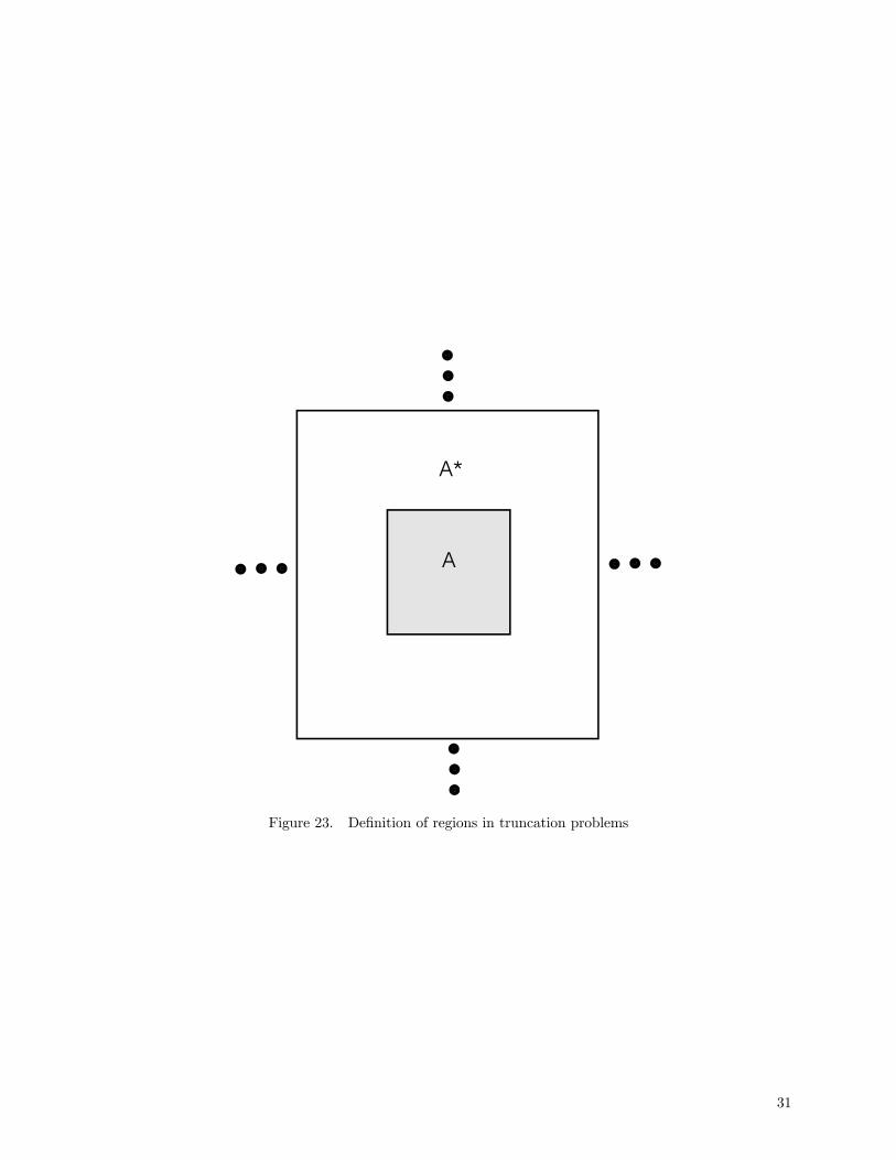
The next group of papers are attempts to improve the knowledge of the current distribution. In thesepapers the researchers start with the solution of the infinite FSS then calculate the difference currentbetween the actual and the infinite FSS current. We will use these methods later in Section 4.1 to scopehow much the current near a seam varies from the infinite FSS current. Figure 23 shows some definitionsthat are useful in the discussion that follows. We have two areas A and A∗ that together make up aninfinite periodic surface. A covers the truncated periodic surface that we are interested in solving, whileA∗ covers the remaining part of the infinite periodic surface.

Munk examines plane wave scattering from an array of dipoles periodic and infinite in one directionand periodic, but finite in the other direction [29]. Although this paper is not focused on the method ofsolving a truncated array, he describes the solution as first finding the currents on the unit cell of an infinitearray (A ∪A∗ in Figure 23). He then adds two semi-infinite arrays of these known currents (but in thenegative direction to the original currents) in the area outside the original finite array (A∗ in Figure 23)cancelling the currents in this area. The scattered field due to the semi-infinite arrays acts as a source in

30

A

A*

Figure 23. Definition of regions in truncation problems

31

addition to the original plane wave and modifies the current distribution across the finite array to take thefiniteness into account. He solves for the difference current between the actual and infinite array current.Note that although the unknowns are representing a difference current instead of the actual current, thenumber of unknowns required hasn’t changed. In fact, we have added to the work load by needing tocalculate the scattered field due to the semi-infinite, known current arrays. Away from the edge of thetruncation, where the current approaches that of the infinite array, the difference current is approximatelyzero, so the unknowns can be expended only over a few unit cells near the edge of the array. Since thecurrent is approximated as existing only around the fringe of the truncated array, it is often called a “fringecurrent” This approximation is where the computational savings is realized. Munk uses the form of thesolution to catalogue the effect of various parameters on the scattered field and is therefore not interestedin the computational savings.

Neto solves a truncated array of slits in a ground plane by a method of moments solution of an integralequation where the unknown is the difference between the exact current distribution on the truncatedarray and the current distribution of the infinite array [25]. Neto follows essentially the same procedureas Munk in setting up the problem, but calculates the field due to the infinite array solution that exists onA∗ asymptotically using the techniques developed by Capolino [21]. The slits are assumed to be small interms of wavelength so that a single pulse basis function can represent the magnetic current of each slit.The difference current is due to the field diffracted from the edges of the array so the current is expandedin terms of complete domain basis functions across the entire aperture. Each complete domain basisfunction consists of an array of pulses at each slit location modulated by a function based on Capolino’spropagating and evanescent asymptotic expansions. Each edge is represented by one propagating and twoevanescent modes leading to six unknowns representing the current. Neto extends these techniques to solvea truncated, 3D array, where the radiators are discretized by many subdomain basis functions [26]. Theproblem is mainly one of book-keeping. The original rooftop basis functions for the infinite array solutionneed to be grouped to represent the more complicated variation of current across the patch composing theunit cell. Then the complete domain basis functions are formed by multiplying the current on each patchby the diffracted fields from each of four edges and vertices. Although Neto describes the full solution,he applied it to the problem of thin, half-wavelength slots. Cucini implemented Neto’s techniques for atruncated array of rectangular waveguides [27].

Civi also solves a truncated array of short dipole antennas each modeled with a single basis function[28]. Unlike Neto and Cucini, Civi solves for the total current on the array. This makes things moredifficult because the current is no longer confined to the array edges. In the center of the array Civiexpanded in terms of a few complete basis functions based on the form of diffracted fields from the edgesand vertices. Since he was working with total currents he also has to include the infinite array Floquetcurrent. On the edges and corners, he expands in terms of subdomain basis functions.

Instead of solving for the currents on a truncated array, Hurst obtains the diffraction coefficient ofa truncated FSS numerically [30]. Admittedly Hurst concentrates mostly on solving for the diffractioncoefficients of a single large strip. He writes the field as a sum of geometric optics field (scattered fromthe center portion of the strip) and two cylindrical waves (scattered from the edges of the strip). Each ofthese contributions has unknown coefficients, but known behavior as a function of distance. He moveshis observation point away from the specular direction so he gets contributions only from the edges (twounknowns). He then separately calculates the field due to two strips of different widths giving him twoequations to solve the two unknowns. The strips must be wide enough to isolate the two edge scatteringcenters, but small enough to be solved numerically. He can then use the diffraction coefficients to solvelarger problems. He uses this technique to obtain the diffraction coefficient of a 20 element strip arrayderiving the diffraction coefficients from solutions of 8 and 9 element strip arrays. The use of stripsbypasses much of the complexity of a 3d array, but this technique looks promising for obtaining thescattering coefficient of a seam.

32

3 The Defect Problem

3.1 Description of GIFFT

Since straightforward numerical analyses of large, finite structures (i.e., explicitly meshing andcomputing interactions between all mesh elements of the entire structure) involve significant memorystorage and computation times, much effort is currently being expended on developing techniques thatminimize the high demand on computer resources. One such technique that belongs to the class offast solvers for large periodic structures is the GIFFT algorithm, which is first discussed in [11]. Thismethod is a modification of the Adaptive Integral Method (AIM) [13], which is a technique based on theprojection of subdomain basis functions onto a rectangular grid. Like the methods presented in [32]-[35],the GIFFT algorithm extends AIM by using basis-function projections onto a rectangular grid throughLagrange interpolating polynomials. The use of a rectangular grid results in a matrix-vector product thatis convolutional in form and can thus be evaluated using FFTs. Although GIFFT differs from [32]-[35] invarious respects, the primary differences between the AIM approach [13] and this method is the latter’suse of interpolation to represent the Green’s function (GF) and its specialization to periodic structures bytaking into account the reusability properties of matrices that arise from interactions between identical cellelements. In GIFFT, the GF projections serve as an approximation of the GF across the periodic structureand the projections of the basis functions are then performed by taking an inner product of the basisfunction with the interpolating polynomials. The GIFFT approach reduces matrix-fill time and memoryrequirements, since interactions between sufficiently-separated, periodic elements can be carried out usinga relatively coarse interpolation of the GF and because only the near element interactions need to beexplicitly calculated. The periodic grid can also be used in a 2D or 3D FFT to accelerate the computationof matrix-vector products used in an iterative solver [13] and indeed, has been shown to greatly reduce solvetime by speeding the matrix-vector product computation.

Fast multipole methods (FMM) [36]-[38] have also been effectively applied to model large structures. Inaddition, a general numerical scheme has been introduced in [39] that uses FMM to determine the couplingbetween periodic cells, with the interior of each cell being analyzed by the finite element method.

The present work extends the GIFFT algorithm to allow for a complete numerical analysis of aperiodic structure with defects as shown in Figure 24. Although GIFFT [11] was originally developedto handle strictly periodic structures, the technique has now been extended to efficiently handle a smallnumber of distinct element types. Thus, in addition to reducing the computational burden associated withlarge periodic structures, GIFFT now permits modeling these structures with source and defect elements.Relaxing the restriction to strictly identical periodic elements is, of course, useful for practical applicationswhere, for example, a dipole excitation may be of interest or, as is often the case for meta-materials,defective elements are introduced in the structure’s fabrication process. The main extensions of the GIFFTmethod compared to [11] are the following:

1. Both periodic “background” and “source” or “defect” elements are now separately defined in translatableunit cells so that in the algorithm, mutual electromagnetic interactions can be computed.

2. The near-interaction block matrix must allow for the possibility of “background-to-source” or“background-to-defect” cell interactions.

3. Matrices representing projections of both “background and source” or “background and defect”subdomain bases onto the interpolation polynomials must be defined and appropriately selected informing the matrix-vector product.

Although here we consider a meta-material layer with a dipole-antenna excitation, as per the extendedGIFFT algorithm, “defect” elements could be considered as well.

33

dipole source y

z

x

Figure 24. Typical geometry of the problems analyzed. A dipole antenna is placed over a periodic artificialmaterial of finite size. A metamaterial structure is formed using two layers of capacitively-loaded split ringresonators (SRRs).

34

1r3r

th cell

m th test function

n th basis function

th cell

2r

p′

p1s

n′pΛ

mpΛ

x

y z th interpolation i

th interpolation′i

2s

Figure 25. Cell index definitions and arbitrary skew lattice vectors. The periodic grid on which the Green’sfunction is evaluated and sampled is shown superimposed on the cells of the periodic structure. Within a3D cell, the Green’s function is evaluated at r1 × r2 × r3 points. The lattice vectors s1 and s2 shown aboveare along x and y, but they can, in general, be along arbitrary directions lying in the xy plane.

In [11] the GIFFT method is applied to periodic structures (arrays, in particular) with polygonalboundaries. Only one element of the array is meshed and provided as input, while all other array elementsare accounted for by taking advantage of the reusability properties of periodic structures comprisingidentical elements. The algorithm is summarized in the following paragraphs, where we use a block-matrixnotation associated with a periodic block of the array.

Referring to Figure 25, the displacement between the p th and pth periodic structure cells is(p1 − p01)

−→s 1 + (p2 − p02)−→s 2 where −→s 1 and −→s 2 are two arbitrary lattice vectors lying in the xy plane. (We

use bold letters to denote both vectors and double indices, and a caret to denote unit vectors.) The vectorr = ρ+ zbz, with ρ = xbx+ yby, is in cell p = (p1, p2) and r0 = ρ0 + z0bz is in cell p0 = (p01, p02). The structuralelements within cells p and p are discretized, for instance, using standard Rao-Wilton-Glisson (RWG) [40]basis functions, with primed and unprimed indices denoting source and testing functions, respectively.

Since in this paper we deal only with scatterers in free space, the moment matrix for the originaldiscretized electric field integral equation (EFIE) can be written as

hZpp

0mn

i hIp

0n

i= [V p

m] (1)

in an obvious generalization of matrix vector products, and with

Zpp0

mn = −DΛpm (r) ;GE (ρ− ρ0, z, z0) ;Λp

0n (r

0)E

(2)

where Λp0n (r

0) and Λpm (r) are RWG basis and testing functions, respectively. For elements separated by atleast one cell, i.e., with p and p0 that satisfy

h¯p1 − p

01

¯,¯p2 − p

02

¯i≡°°°p− p0°°° > 1, we approximate the GF

GE (ρ− ρ0, z, z0) via Lagrange polynomial interpolation as

GE (ρ− ρ0, z, z0) uXi,i0,j,j0

Li (ρ)Lj (z)GEi−i0,j,j0Li0 (ρ0)Lj0 (z0) (3)

where the indices on GEi−i0,j,j0 ≡ GE³ρ(i) − ρ0(i0), z(j), z0(j0)

´denote sampled values of the coordinates and

Li (ρ)Lj (z) are Lagrange interpolation polynomials defined on the interpolation points within a cell shownin Figure 25 (i is a double index i = (i1, i2)) . It is significant that in the evaluation of the interaction Zpp

0mn

35

between two cells p and p0, the interpolation scheme generally requires many fewer GF evaluations per

cell than the usual case where subdomain interactions are evaluated directly, or even than the usual AIMapproach requires. This becomes especially true as the complexity of the geometry within a cell increasesor when GFs for layered media are used.

In the GIFFT formulation, the GF interpolation in (3) is used so that the (m,n)th element in thematrix block Zpp

0mn (see (2)) may be represented as

Zpp0

mn ≈ eZpp0mn = −Xi,i0,j,j0

hΛpm (r) , Li (ρ)Lj (z)i · GEi−i0,j,j0 ·DLi0 (ρ

0)Lj0 (z0) ,Λp0

n (r0)E

(4)

where p and p0correspond to the testing and source cells and the tilde denotes an approximated block of

the impedance matrix. Since a low-order interpolation of the Green’s function is not accurate near thesource point, Equation 6 is not sufficiently accurate when the cell (index) separation is too small. To avoidthis inaccuracy while minimizing the number of interpolating polynomials within each cell, the self-blockcoupling and that between adjacent neighbor blocks is found by standard Method of Moments techniques(MoM). With good accuracy, the original discretized EFIE in (1) is thus rewritten as

h∆Zpp

0mn

i hIp

0n

i+h eZpp0mn

i hIp

0n

i= [V p

m] (5)

where the block Toeplitz difference matrix ∆Zpp0

mn = Zpp0

mn − eZpp0mn is assumed to vanish for elements

satisfying maxh¯p1 − p

01

¯,¯p2 − p

02

¯i> 1, and hence is sparse. We also note that generally GEi−i0,j,j0 = ∞

when i = i0, j = j0 inh∆Zpp

0mn

iand

h eZpp0mn

i. Since, for convenience, Equation 5 is applied over the entire

impedance matrix, the infinite values occurring inh∆Zpp

0mn

iand

h eZpp0mn

iwhen i = i0, j = j0 are replaced

with finite values, with the net contribution due to the two terms being equal to zero. To evaluate the

matrix-vector product, we note that the producth∆Zpp

0mn

i hIp

0n

ican be performed efficiently since

h∆Zpp

0mn

iis sparse, whereas

h eZpp0mn

i hIp

0n

iis of convolutional form and can be evaluated quickly using a 2D FFT.

More specifically,

h eZpp0mn

i hIp

0n

i= (6)

−Xi,,j,j0

hΛpm (r) , LiLji ·MASKiFFT−1i

⎡⎣FFTi ³GEi,j,j0´ · FFTi⎛⎝X

p0

NXn=1

DLiLj0 ,Λ

p0n (r0)

EIp

0n

⎞⎠⎤⎦where the double bars over a quantity indicate that its length is extended and appropriately zero-padded soas to obtain a circular convolutional form of vectors of length 2k for applying the FFT. The term FFT−1

denotes the inverse fast Fourier transform and MASKi is a mask that restricts the result to cells withinthe structure’s polygonal boundary. The degree to which Equation 5 approximates Equation 1 depends on

how many elements are chosen to be different from zero inh∆Zpp

0mn

i(the strong-interaction matrix) and on

how many interpolation points are used forh eZpp0mn

i. It has been consistently found that setting ∆Zpp

0mn = 0

for interactions between p and p0elements such that max

h¯p1 − p

01

¯,¯p2 − p

02

¯i> 1 provides good accuracy.

The GIFFT method has been incorporated into one version of the frequency-domain MoM EIGER codesuite [42]. This was done to preserve many of the features of EIGER and to reduce development time.

36

y h

Figure 26. Periodic structure cells for a square lattice, with periods a and b that, for a metamaterialstructure, are much smaller than the wavelength. The source is located at the upper right corner of themother cell p0 = (0, 0), and both exact and interpolated GFs are evaluated in the cell p = (1, 1). The dotsrepresent Green’s function sampling points over a cell cross section.

EIGER has been adapted for efficiently running large array or large FSS’s with either identical or varyingunit-cell geometry (allowing for the simulation of defects in the periodic structures) with the resulting codebeing referred to in the following sections as EIGER_GIFFT. GIFFT is presently in the process of beingincorporated into the official version of EIGER.

3.2 Modeling Sources Using GIFFT

The GIFFT method requires that only distinct cell geometries be meshed and provided as input tothe electromagnetic solver code. For very large structures this has the advantage of condensing the inputdata and reduces the chance of introducing mesh errors for complex structures. Thus, to model a dipolesource over a finite meta-material layer, we provide GIFFT the geometry for two distinct structures. Thefirst consists of the mesh geometry for unit cells making up the “background” meta-material layer. For thestructure shown Figure 24, the “background” unit cell can be taken as two split-ring resonators (SRRs)oriented along the bz direction. The second geometry description is that of the unit cell containing a singledipole plus two SRR elements (the “source” element). For the GIFFT technique, only the explicit meshingof these two distinct unit cells is required, with a replication of these “mother” cells automatically occurringin the computational part of the algorithm. (For the structure shown in Figure 24, we have one “source”element and 24 “background” elements). It is significant to note that, for this implementation, the GFsampling grid has to be large enough to include both “background” and “source” elements (independentlyof their location) to form a large brick volume (only the yz plane is shown in Figure 26) where the FFTalgorithm is then applied.

3.3 Accuracy of the Green’s Function Approximation and Interpolation

To date, the GIFFT method has been applied to array antenna configurations where the distancesbetween the antenna elements, and thus the size of the array cells, are on the order of a half wavelength.A graph of GF interpolation error for such array elements shown in [11] permits the determination of thenumber of GF interpolation points needed within a cell to guarantee a certain degree of GF approximation.One would expect that meta-material lattices characterized by unit cells much smaller than a wavelengthshould no pose particular problems since, in general, it is easier to approximate a quasi-static kernel (GF)than an oscillatory one. Hence, the data in [11] should serve as an upper bound for cell sizes that canbe approximated efficiently. Furthermore, for cell sizes small relative to a wavelength, the approximationnecessarily becomes frequency independent, since quasi-static approximation accuracy depends only on celldimension to separation ratios.

The precise upper bound of the error for the meta-material geometry treated in this paper, with latticeperiods a = 1.57 mm and b = 5.08 mm, has been checked by evaluating both approximated and exact GFs

37

′p

p

x

y a

b

Figure 27. Periodic structure cells for a square lattice with periods a and b that, for a metamaterialstructure, are much smaller than the wavelength. The source is located at the upper right corner of themother cell p0 = (0, 0) and both exact and interpolated Green’s functions are evaluated in the cell p = (2, 1).

on the cell p = (2, 1) depicted in Figure 27, with height (along the bz direction) equal to b, and with asource located at the upper right corner of the mother cell p0 = (0, 0). This is a worst-case scenario for ourgeometry where b > a. For a 3× 7× 7 grid (along bx, by, and bz) of interpolation points per block, accuracyin the GF of at least three significant figures is obtained within the cell under consideration. Note that theSRR dimensions are such that they do not extend to the edge of the periodic cell (where we have locatedthe source in Figure 27) and therefore the expected accuracy for our example problem is even slightlybetter. This check shows that the use of a 3× 7× 7 sampling grid is sufficient to assure that Zpp0mn equalseZpp0mn to at least three significant figures when either

¯p1 − p

01

¯> 1 or

¯p2 − p

02

¯> 1.

3.4 Analysis of a Dipole Over a High Impedance Surface

3.4.1 Meta-material of Infinite Periodic Extent

An infinite-periodic material made of a two layer array of capacitively-loaded SRRs is studied here forbroadside plane-wave illumination propagating along the −bz direction. With the exception of the dipoleexcitation, the finite counterpart of this structure is shown in Figure 24. The SRR geometry is shownin Figure 28 where the dimensions are given by W = 4.06, L = 2.54, T = 0.457, U = 1.65, S = 1.245,G1 = 1.02 and G2 = 0.508 (units all in mm). As mentioned previously, the basic unit cell (considered the“background” unit cell in the finite array analysis) consists of two SRRs oriented along the bz directionand with the capacitive gaps facing the incoming plane wave. A similar SRR-based meta-material block,of both infinite and finite extent, has been studied by Erentok et al. in [41] and shown to provide goodartificial-magnetic-conductor (AMC) performance, with demonstrated agreement between experiment andsimulations. While in [41] these SRR elements were embedded in a Duroid substrate of εr = 2.2, for apreliminary application of the GIFFT method an air substrate is first considered since it permits use of theFFT in all three dimensions. The periodicity along the x and y directions of the meta-material layer aretaken to be 1.57 mm and W +G1 = 5.08 mm, respectively.

As is well known, the reflection coefficient associated with such a periodic material is defined by thescattered dominant Floquet wave with phase reference at z = 0 (which in this study is coincident with thetop of the SRR unit cell). For this portion of the study, a standard MoM code (EIGER [11],[42],[43]) wasused to determine the reflection coefficient characterizing the infinite meta-material structure. With theresults shown in Figure 29, it is evident that above 12 GHz the magnitude of the reflection coefficient is

38

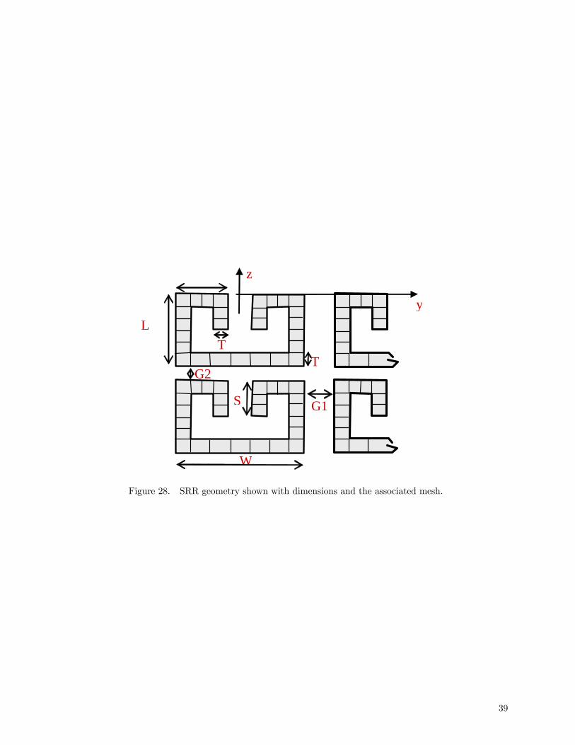
z

y

G1

T L

G2 T

S

W

Figure 28. SRR geometry shown with dimensions and the associated mesh.

39

8.0 9.0 10.0 11.0 12.0 13.0 14.0 15.0 16.0 17.0 18.0Frequency [GHz]

-180

-90

0

90

180

Phase [degrees]

0.0

0.2

0.4

0.6

0.8

1.0

Mag

nitu

de

Broadside (Phase S11, 1 Quad)Broadside (Phase S11, 3 Quads)Broadside (Amplitude S11, 1 Quad)Broadside (Amplitude S11, 3 Quads)

Figure 29. Results characterizing the reflection coefficient for a plane wave impinging from broadside usingtwo meshes with a varying number of quadrilaterals modeling the SRR thickness (see Figure 28). Meshconvergence is demonstrated at f = 15.7 GHz, where the magnitude of the reflection coefficient is equal tounity and a zero-crossing of the phase (at a reference plane)

nearly unity, with the zero-crossing of the phase (at the reference plane z = 0) occurring at f = 15.7 GHz.Thus, at this frequency and for this particular unit-cell orientation, the SRR-based meta-material layerbehaves likes an AMC. In [41] it is shown that the orientation between the SRR elements and theincident field has a significant effect on the overall layer performance (an AMC versus an artificial-electricconductor). Figure 29 shows that there is a slight difference in the reflection coefficient when a muchfiner mesh is used to model the SRRs. In order to ensure that the capacitive effect of the resonators wascaptured, the number of quadrilateral elements modeling the thickness of the SRRs ( T in Figure 28) wasincreased from one to three. Since very little change occurs near the AMC frequency, mesh convergence isdemonstrated.

3.4.2 Meta-material of Finite Extent with a Source Excitation

A short strip dipole is placed at a height h above the top of the upper SRR, as shown in Figures 24 and26. The flat strip dipole is placed in the xy plane (zero thickness along bz) and is of width W = 0.4 mm inthe bx direction and length L = 2.4 mm along the by direction. It is fed by a delta-gap voltage generator atits center and meshed with three basis functions along its length.

As a first means of assessing the performance of the GIFFT method, a moderate-sized SRRmeta-material of 9 × 7 cells along bx and by with two SRRs along the bz direction for each cell is analyzedusing both the GIFFT technique and a standard Toeplitz MoM method. The strip dipole is placed ath = 2.5 mm above the top part of the top SRR. The average current density associated with each unitcell (including both the top and bottom SRR shown in Figure 28), predicted from both methods, is shownin Figure 30 at a frequency f = 13.8 GHz. Here the current density is plotted versus the cell numberin the array, where the cell numbering in GIFFT proceeds from #1 for the lower leftmost unit-cell andproceeding across from left to right. The strip-dipole placement above the center of the meta-material block(as assumed throughout this study) is, for this structure, located in cell #32. Figure 30 demonstrates good

40

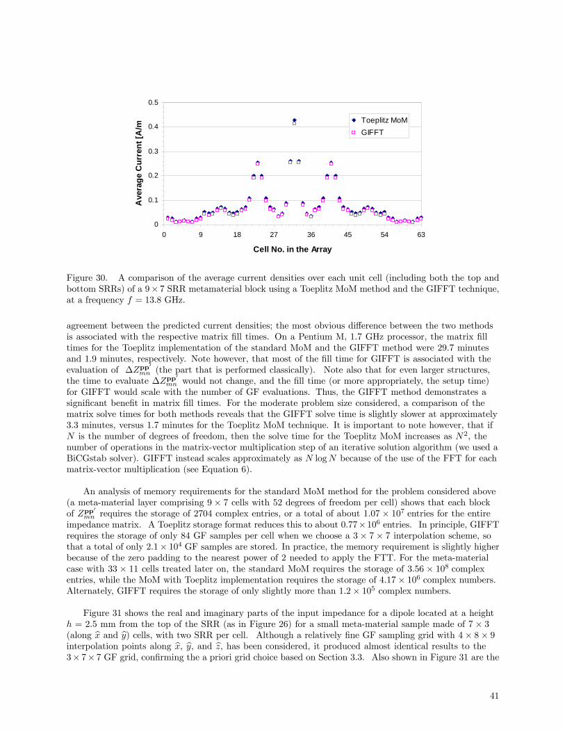
0

0.1

0.2

0.3

0.4

0.5

0 9 18 27 36 45 54 63

Cell No. in the Array

Ave

rage

Cur

rent

[A/m

Toeplitz MoM GIFFT

Figure 30. A comparison of the average current densities over each unit cell (including both the top andbottom SRRs) of a 9× 7 SRR metamaterial block using a Toeplitz MoM method and the GIFFT technique,at a frequency f = 13.8 GHz.

agreement between the predicted current densities; the most obvious difference between the two methodsis associated with the respective matrix fill times. On a Pentium M, 1.7 GHz processor, the matrix filltimes for the Toeplitz implementation of the standard MoM and the GIFFT method were 29.7 minutesand 1.9 minutes, respectively. Note however, that most of the fill time for GIFFT is associated with theevaluation of ∆Zpp

0mn (the part that is performed classically). Note also that for even larger structures,

the time to evaluate ∆Zpp0

mn would not change, and the fill time (or more appropriately, the setup time)for GIFFT would scale with the number of GF evaluations. Thus, the GIFFT method demonstrates asignificant benefit in matrix fill times. For the moderate problem size considered, a comparison of thematrix solve times for both methods reveals that the GIFFT solve time is slightly slower at approximately3.3 minutes, versus 1.7 minutes for the Toeplitz MoM technique. It is important to note however, that ifN is the number of degrees of freedom, then the solve time for the Toeplitz MoM increases as N2, thenumber of operations in the matrix-vector multiplication step of an iterative solution algorithm (we used aBiCGstab solver). GIFFT instead scales approximately as N logN because of the use of the FFT for eachmatrix-vector multiplication (see Equation 6).

An analysis of memory requirements for the standard MoM method for the problem considered above(a meta-material layer comprising 9 × 7 cells with 52 degrees of freedom per cell) shows that each blockof Zpp

0mn requires the storage of 2704 complex entries, or a total of about 1.07 × 107 entries for the entire

impedance matrix. A Toeplitz storage format reduces this to about 0.77×106 entries. In principle, GIFFTrequires the storage of only 84 GF samples per cell when we choose a 3 × 7 × 7 interpolation scheme, sothat a total of only 2.1× 104 GF samples are stored. In practice, the memory requirement is slightly higherbecause of the zero padding to the nearest power of 2 needed to apply the FTT. For the meta-materialcase with 33 × 11 cells treated later on, the standard MoM requires the storage of 3.56 × 108 complexentries, while the MoM with Toeplitz implementation requires the storage of 4.17× 106 complex numbers.Alternately, GIFFT requires the storage of only slightly more than 1.2× 105 complex numbers.

Figure 31 shows the real and imaginary parts of the input impedance for a dipole located at a heighth = 2.5 mm from the top of the SRR (as in Figure 26) for a small meta-material sample made of 7 × 3(along bx and by) cells, with two SRR per cell. Although a relatively fine GF sampling grid with 4× 8× 9interpolation points along bx, by, and bz, has been considered, it produced almost identical results to the3× 7× 7 GF grid, confirming the a priori grid choice based on Section 3.3. Also shown in Figure 31 are the

41

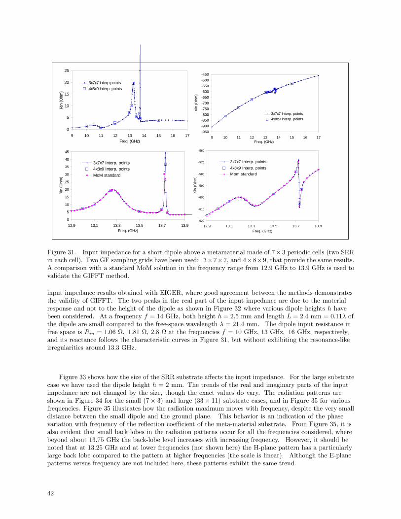
0

5

10

15

20

25

9 10 11 12 13 14 15 16 17Freq. (GHz)

Rin

(Ohm

)

3x7x7 Interp points4x8x9 Interp. points

-950-900-850-800-750-700-650-600-550-500-450

9 10 11 12 13 14 15 16 17Freq. (GHz)

Xin

(Ohm

)

3x7x7 Interp. points4x8x9 Interp. points

0

5

10

15

20

25

30

35

40

45

12.9 13.1 13.3 13.5 13.7 13.9Freq. (GHz)

Rin

(Ohm

)

3x7x7 Interp. points4x8x9 Interp. pointsMoM standard

-620

-610

-600

-590

-580

-570

-560

12.9 13.1 13.3 13.5 13.7 13.9Freq. (GHz)

Xin

(Ohm

)

3x7x7 Interp. points4x8x9 Interp. pointsMom standard

Figure 31. Input impedance for a short dipole above a metamaterial made of 7× 3 periodic cells (two SRRin each cell). Two GF sampling grids have been used: 3×7×7, and 4×8×9, that provide the same results.A comparison with a standard MoM solution in the frequency range from 12.9 GHz to 13.9 GHz is used tovalidate the GIFFT method.

input impedance results obtained with EIGER, where good agreement between the methods demonstratesthe validity of GIFFT. The two peaks in the real part of the input impedance are due to the materialresponse and not to the height of the dipole as shown in Figure 32 where various dipole heights h havebeen considered. At a frequency f = 14 GHz, both height h = 2.5 mm and length L = 2.4 mm = 0.11λ ofthe dipole are small compared to the free-space wavelength λ = 21.4 mm. The dipole input resistance infree space is Rin = 1.06 Ω, 1.81 Ω, 2.8 Ω at the frequencies f = 10 GHz, 13 GHz, 16 GHz, respectively,and its reactance follows the characteristic curves in Figure 31, but without exhibiting the resonance-likeirregularities around 13.3 GHz.

Figure 33 shows how the size of the SRR substrate affects the input impedance. For the large substratecase we have used the dipole height h = 2 mm. The trends of the real and imaginary parts of the inputimpedance are not changed by the size, though the exact values do vary. The radiation patterns areshown in Figure 34 for the small (7× 3) and large (33× 11) substrate cases, and in Figure 35 for variousfrequencies. Figure 35 illustrates how the radiation maximum moves with frequency, despite the very smalldistance between the small dipole and the ground plane. This behavior is an indication of the phasevariation with frequency of the reflection coefficient of the meta-material substrate. From Figure 35, it isalso evident that small back lobes in the radiation patterns occur for all the frequencies considered, wherebeyond about 13.75 GHz the back-lobe level increases with increasing frequency. However, it should benoted that at 13.25 GHz and at lower frequencies (not shown here) the H-plane pattern has a particularlylarge back lobe compared to the pattern at higher frequencies (the scale is linear). Although the E-planepatterns versus frequency are not included here, these patterns exhibit the same trend.

42

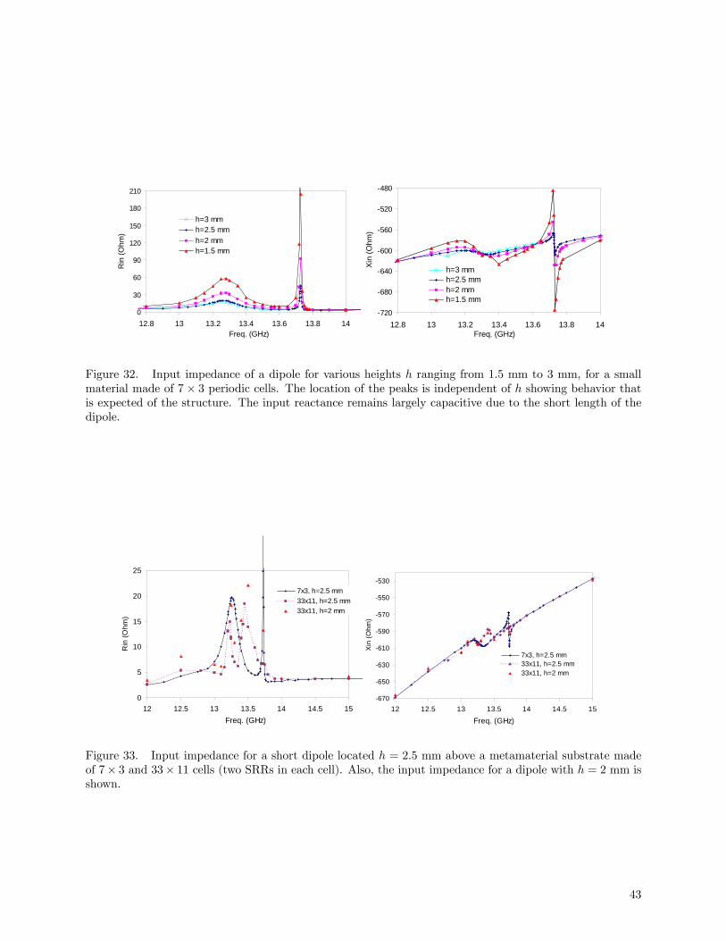
0

30

60

90

120

150

180

210

12.8 13 13.2 13.4 13.6 13.8 14Freq. (GHz)

Rin

(Ohm

)

h=3 mmh=2.5 mmh=2 mmh=1.5 mm

-720

-680

-640

-600

-560

-520

-480

12.8 13 13.2 13.4 13.6 13.8 14Freq. (GHz)

Xin

(Ohm

)

h=3 mmh=2.5 mmh=2 mmh=1.5 mm

Figure 32. Input impedance of a dipole for various heights h ranging from 1.5 mm to 3 mm, for a smallmaterial made of 7× 3 periodic cells. The location of the peaks is independent of h showing behavior thatis expected of the structure. The input reactance remains largely capacitive due to the short length of thedipole.

0

5

10

15

20

25

12 12.5 13 13.5 14 14.5 15Freq. (GHz)

Rin

(Ohm

)

7x3, h=2.5 mm33x11, h=2.5 mm33x11, h=2 mm

-670

-650

-630

-610

-590

-570

-550

-530

12 12.5 13 13.5 14 14.5 15Freq. (GHz)

Xin

(Ohm

)

7x3, h=2.5 mm33x11, h=2.5 mm33x11, h=2 mm

Figure 33. Input impedance for a short dipole located h = 2.5 mm above a metamaterial substrate madeof 7× 3 and 33× 11 cells (two SRRs in each cell). Also, the input impedance for a dipole with h = 2 mm isshown.

43

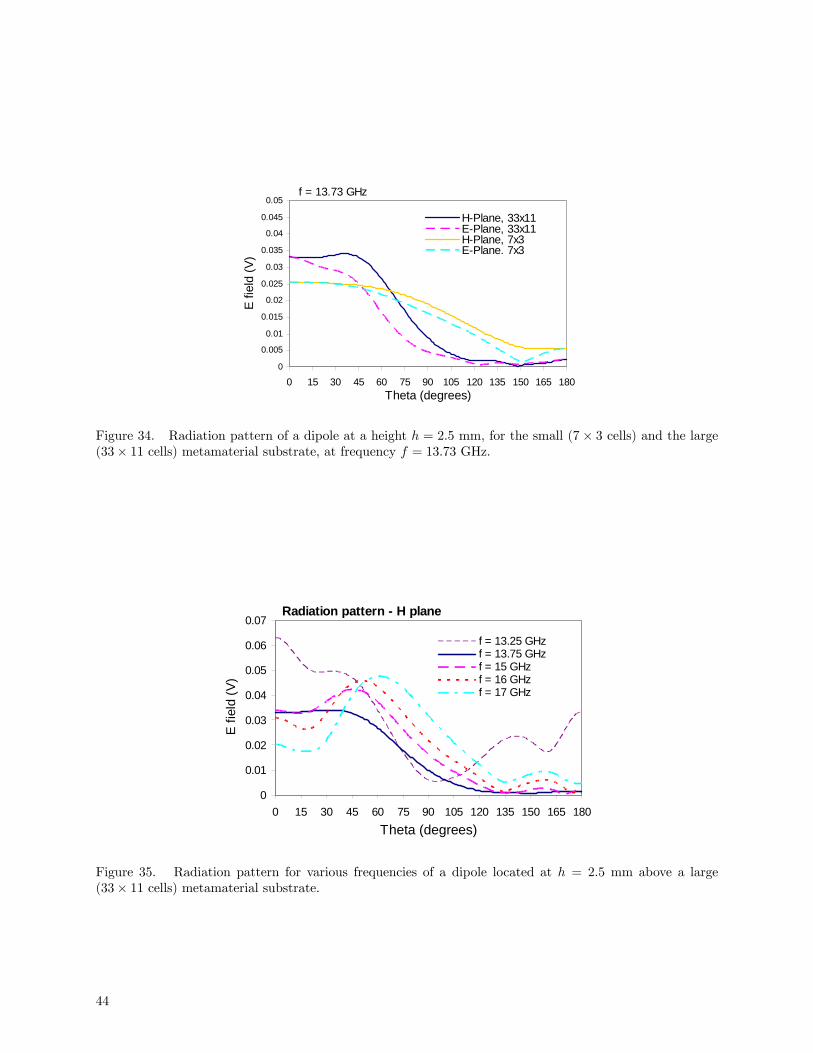
f = 13.73 GHz

0

0.005

0.01

0.015

0.02

0.025

0.03

0.035

0.04

0.045

0.05

0 15 30 45 60 75 90 105 120 135 150 165 180Theta (degrees)

E fi

eld

(V)

H-Plane, 33x11E-Plane, 33x11H-Plane, 7x3 E-Plane, 7x3

Figure 34. Radiation pattern of a dipole at a height h = 2.5 mm, for the small (7× 3 cells) and the large(33× 11 cells) metamaterial substrate, at frequency f = 13.73 GHz.

Radiation pattern - H plane

0

0.01

0.02

0.03

0.04

0.05

0.06

0.07

0 15 30 45 60 75 90 105 120 135 150 165 180Theta (degrees)

E fie

ld (V

)

f = 13.25 GHzf = 13.75 GHzf = 15 GHzf = 16 GHzf = 17 GHz

Figure 35. Radiation pattern for various frequencies of a dipole located at h = 2.5 mm above a large(33× 11 cells) metamaterial substrate.

44

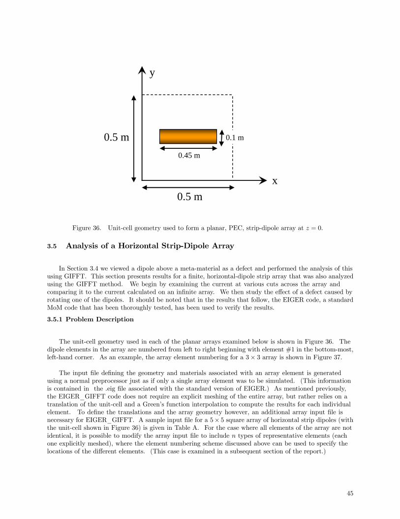
0.5 m

0.5 m x

y

0.45 m

0.1 m

Figure 36. Unit-cell geometry used to form a planar, PEC, strip-dipole array at z = 0.

3.5 Analysis of a Horizontal Strip-Dipole Array

In Section 3.4 we viewed a dipole above a meta-material as a defect and performed the analysis of thisusing GIFFT. This section presents results for a finite, horizontal-dipole strip array that was also analyzedusing the GIFFT method. We begin by examining the current at various cuts across the array andcomparing it to the current calculated on an infinite array. We then study the effect of a defect caused byrotating one of the dipoles. It should be noted that in the results that follow, the EIGER code, a standardMoM code that has been thoroughly tested, has been used to verify the results.

3.5.1 Problem Description

The unit-cell geometry used in each of the planar arrays examined below is shown in Figure 36. Thedipole elements in the array are numbered from left to right beginning with element #1 in the bottom-most,left-hand corner. As an example, the array element numbering for a 3× 3 array is shown in Figure 37.

The input file defining the geometry and materials associated with an array element is generatedusing a normal preprocessor just as if only a single array element was to be simulated. (This informationis contained in the .eig file associated with the standard version of EIGER.) As mentioned previously,the EIGER_GIFFT code does not require an explicit meshing of the entire array, but rather relies on atranslation of the unit-cell and a Green’s function interpolation to compute the results for each individualelement. To define the translations and the array geometry however, an additional array input file isnecessary for EIGER_GIFFT. A sample input file for a 5× 5 square array of horizontal strip dipoles (withthe unit-cell shown in Figure 36) is given in Table A. For the case where all elements of the array are notidentical, it is possible to modify the array input file to include n types of representative elements (eachone explicitly meshed), where the element numbering scheme discussed above can be used to specify thelocations of the different elements. (This case is examined in a subsequent section of the report.)

45

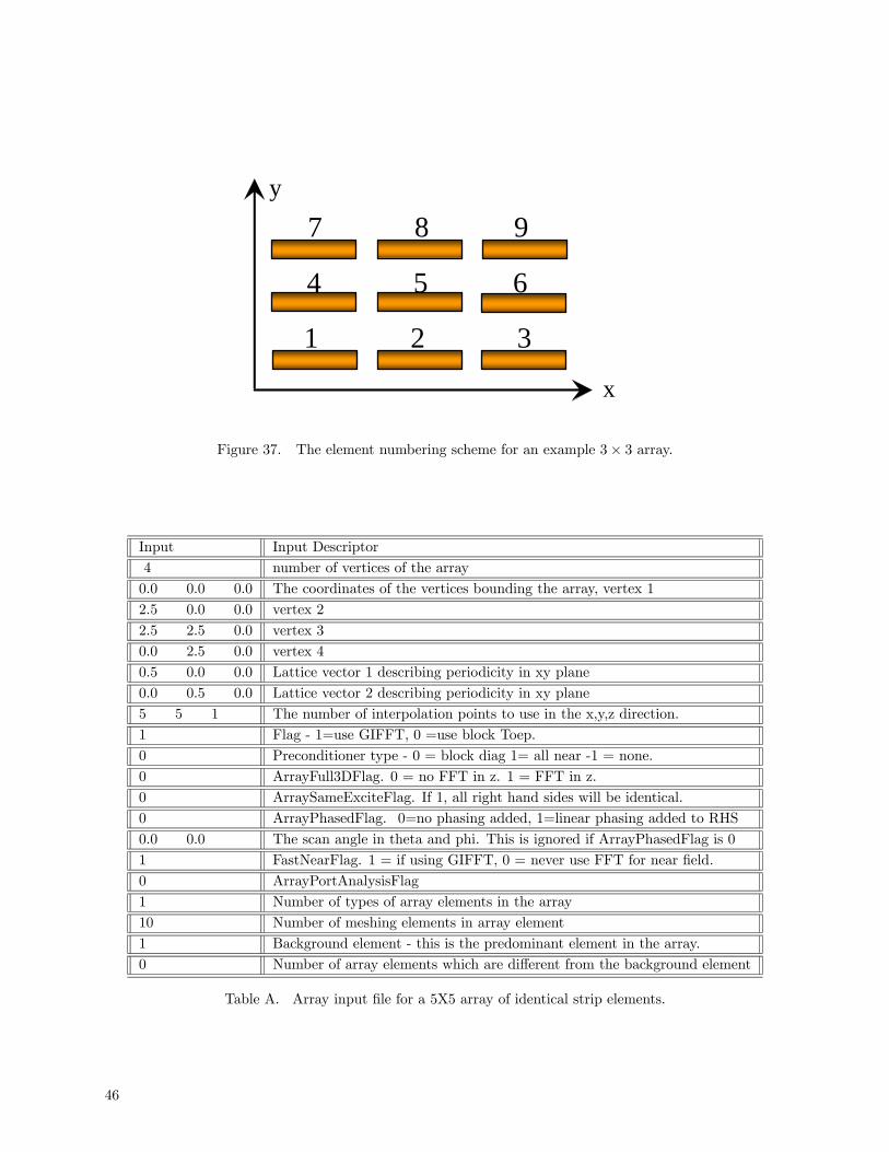
1 2 3

4 5 6

7 8 9

x

y

Figure 37. The element numbering scheme for an example 3× 3 array.

Input Input Descriptor4 number of vertices of the array0.0 0.0 0.0 The coordinates of the vertices bounding the array, vertex 12.5 0.0 0.0 vertex 2

2.5 2.5 0.0 vertex 30.0 2.5 0.0 vertex 40.5 0.0 0.0 Lattice vector 1 describing periodicity in xy plane0.0 0.5 0.0 Lattice vector 2 describing periodicity in xy plane5 5 1 The number of interpolation points to use in the x,y,z direction.1 Flag - 1=use GIFFT, 0 =use block Toep.0 Preconditioner type - 0 = block diag 1= all near -1 = none.0 ArrayFull3DFlag. 0 = no FFT in z. 1 = FFT in z.0 ArraySameExciteFlag. If 1, all right hand sides will be identical.0 ArrayPhasedFlag. 0=no phasing added, 1=linear phasing added to RHS

0.0 0.0 The scan angle in theta and phi. This is ignored if ArrayPhasedFlag is 01 FastNearFlag. 1 = if using GIFFT, 0 = never use FFT for near field.0 ArrayPortAnalysisFlag1 Number of types of array elements in the array10 Number of meshing elements in array element1 Background element - this is the predominant element in the array.0 Number of array elements which are different from the background element

Table A. Array input file for a 5X5 array of identical strip elements.

46

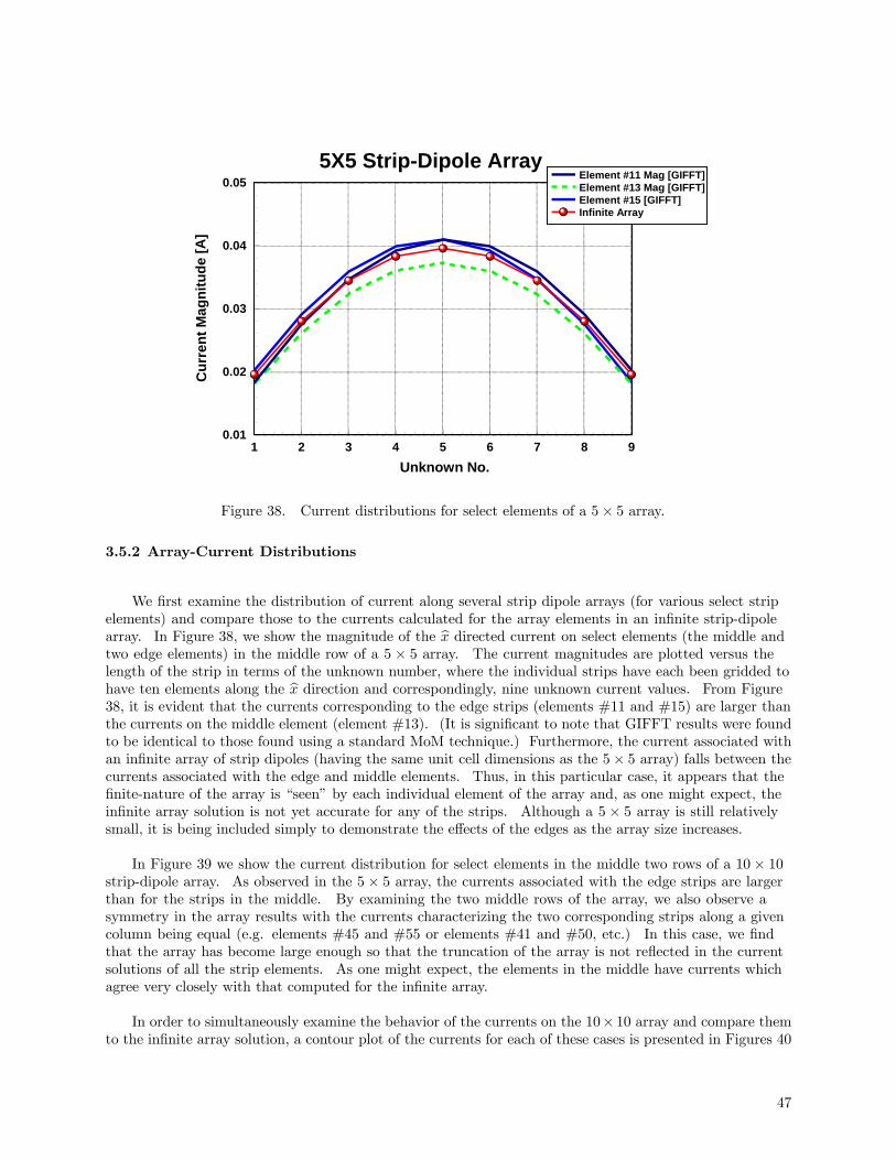
1 2 3 4 5 6 7 8 9Unknown No.

0.01

0.02

0.03

0.04

0.05C

urre

nt M

agni

tude

[A]

Element #11 Mag [GIFFT]Element #13 Mag [GIFFT]Element #15 [GIFFT]Infinite Array

5X5 Strip-Dipole Array

Figure 38. Current distributions for select elements of a 5× 5 array.

3.5.2 Array-Current Distributions

We first examine the distribution of current along several strip dipole arrays (for various select stripelements) and compare those to the currents calculated for the array elements in an infinite strip-dipolearray. In Figure 38, we show the magnitude of the bx directed current on select elements (the middle andtwo edge elements) in the middle row of a 5 × 5 array. The current magnitudes are plotted versus thelength of the strip in terms of the unknown number, where the individual strips have each been gridded tohave ten elements along the bx direction and correspondingly, nine unknown current values. From Figure38, it is evident that the currents corresponding to the edge strips (elements #11 and #15) are larger thanthe currents on the middle element (element #13). (It is significant to note that GIFFT results were foundto be identical to those found using a standard MoM technique.) Furthermore, the current associated withan infinite array of strip dipoles (having the same unit cell dimensions as the 5× 5 array) falls between thecurrents associated with the edge and middle elements. Thus, in this particular case, it appears that thefinite-nature of the array is “seen” by each individual element of the array and, as one might expect, theinfinite array solution is not yet accurate for any of the strips. Although a 5 × 5 array is still relativelysmall, it is being included simply to demonstrate the effects of the edges as the array size increases.

In Figure 39 we show the current distribution for select elements in the middle two rows of a 10× 10strip-dipole array. As observed in the 5 × 5 array, the currents associated with the edge strips are largerthan for the strips in the middle. By examining the two middle rows of the array, we also observe asymmetry in the array results with the currents characterizing the two corresponding strips along a givencolumn being equal (e.g. elements #45 and #55 or elements #41 and #50, etc.) In this case, we findthat the array has become large enough so that the truncation of the array is not reflected in the currentsolutions of all the strip elements. As one might expect, the elements in the middle have currents whichagree very closely with that computed for the infinite array.

In order to simultaneously examine the behavior of the currents on the 10× 10 array and compare themto the infinite array solution, a contour plot of the currents for each of these cases is presented in Figures 40

47

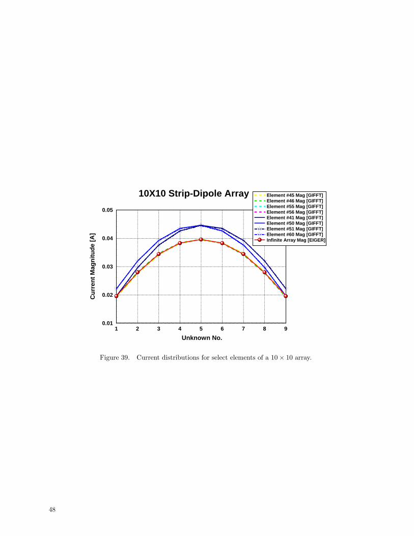
1 2 3 4 5 6 7 8 9Unknown No.

0.01

0.02

0.03

0.04

0.05

Cur

rent

Mag

nitu

de [A

]

Element #45 Mag [GIFFT]Element #46 Mag [GIFFT]Element #55 Mag [GIFFT]Element #56 Mag [GIFFT]Element #41 Mag [GIFFT]Element #50 Mag [GIFFT]Element #51 Mag [GIFFT]Element #60 Mag [GIFFT]Infinite Array Mag [EIGER]

10X10 Strip-Dipole Array

Figure 39. Current distributions for select elements of a 10× 10 array.

48

Figure 40. Contour plot of the current magnitude for an infinite array of the strip dipole shown in Figure36.

and 41. Like the results shown in Figure 39, the currents towards the center of the array are characterizedby the infinite array currents, whereas the elements closer to the edges (along bx) are characterized by highercurrent values (note the respective scales on Figures 40 and 41). Furthermore, from the contour plot inFigure 41 it is possible to observe the current symmetry along the array (along the center of the array.)

Next we increase the size of the array even further to 40 × 40 elements. In Figure 42 we show themagnitude of the current at the strip centers along various rows and columns of the array. Also plotted isthe current associated with the infinite strip array, where the value of the center currents are all identical.Proceeding along the middle row and middle column of the finite array (recognizing that, as shown above,the two center rows and columns have the same current distributions by symmetry), we find that thecurrents agree very well with the infinite array currents for the elements located towards the center of thearray. However, as previously seen in the 10× 10 array, as the position of the dipole gets closer to the edgeof the array, the currents begin to differ from the infinite array solution, with the currents for the edgestrips being the most different. Comparing the results corresponding to the first row and first column tothat of the middle elements, it is interesting to note that the average of these currents approximately yieldsthe values of the currents on the middle strips.

3.5.3 Computational Times

Table B contains some comparisons of the matrix fill and solve times for the GIFFT method and astandard MoM technique, based on the horizontal strip-array problem. These problems were all run ona PC with a XEON 3.0 GHz processor. Due to the Green’s function interpolation, the matrix fill timeassociated with the GIFFT method is significantly lower than the fill time associated with the standardMoM. Comparing a 5× 5 to a 10× 10 array, it is evident that the time savings in the fill-time dramatically

49

Figure 41. Contour plot of the current magnitude for a 10× 10 array of the strip dipole shown in Figure36.

1 6 11 16 21 26 31 36Element No.

0.03

0.04

0.05

0.06

Cur

rent

Mag

nitu

de [A

]

Middle Row (#20)First RowLast Row Infinite Array Mag [Eig_G]Middle Column (#20)First ColumnLast Column

40X40 Strip-Dipole Array

Figure 42. Current distributions for select elements of a 40× 40 array.

50

increases as the size of the problem grows. Since the code using standard MoM has been optimizedfor direct solves while the iterative solver used in the GIFFT code has not, the matrix solve times forGIFFT are currently higher than for EIGER. Nevertheless, due to the significant decrease in fill times,GIFFT is an overall faster method than standard MoM (order N logN vs. N3 for direct solve) and thisis especially true for larger arrays. In addition to comparing the run times associated with the GIFFTand EIGER codes, it is important to note that the preprocessing time associated with the GIFFT code issignificantly less than that for EIGER, where an explicit meshing of the array must be carried out. Sincethe preprocessing time increases dramatically with increasing array size, the explicit meshing of the 40× 40array and hence the time comparison for the two codes was not carried out for this case.

Matrix Fill Time [s] Matrix Solve Time [s]GIFFT [EIGER_GIFFT]5× 5 1.625 0.125Standard MoM [EIGER] 5× 5 89.172 0.07813GIFFT [EIGER_GIFFT]10× 10 1.531 1.484Standard MoM [EIGER]10× 10 704.39 0.1875

Table B. Matrix fill and solve times for a 5× 5 and 10 × 10 element array using GIFFT and the standardMoM.

3.5.4 Defect in a 5× 5 Element Array

In this section of the report, we examine the changes in the array current and radiation pattern asdefect elements are introduced into the array. In Figure 43 the current magnitudes for the middle-rowstrips in the array are presented, where the center element (#13) has been rotated about bz by 45. (Thearray input deck associated with this array geometry is given in Table C.) From Figure 43 we observe that,relative to the array with no defects, the current levels are decreased when keeping the same plane-waveillumination (an bx directed electric field). For comparison purposes, the current results determined usingthe standard MoM code (EIGER) are also shown in Figure 43, where the results are found to be in verygood agreement.

In Figure 44, the θ polarization of the far-zone electric field (Eθ in the E-plane) is shown for the twocases of a perfectly-aligned 5 × 5 array and one where the center element has been tilted by 45. Whilethis single defect (a point defect) results in little change in Eθ , the presence of the defect creates an Eϕ

pattern where none existed previously. This is as expected due to the 45 orientation of the excitedcurrents on the rotated dipole, where previously the currents flowed only along the bx direction. The Eϕ

pattern characterizing the array with the defect element is presented in Figure 45.

3.6 Conclusion and Future Work on Defects

The GIFFT method has been generalized to enable the treatment of source structures embedded in aperiodic background of finite size. As an example, the GIFFT method was applied to the case of a shortdipole source above an artificial material made of two layers of capacitively loaded SRRs. The problemillustrates the variety of results one can obtain with small and large meta-material substrates of finite size,structures where the large number of unknowns typically make such problems computationally challenging.In this analysis, sources (and/or defects) in other meta-materials made by a periodic arrangement of otherresonant or nonresonant subwavelength structures could be treated as well. The present contributionis devoted to scatterers in free space; inclusions in a multilayer environment will be treated in futureinvestigations. GIFFT was also used to examine large, truncated FSS’s and single point defects.

51

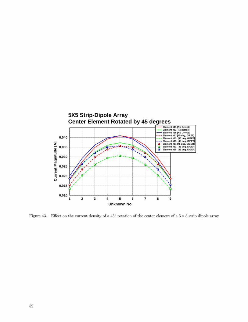
1 2 3 4 5 6 7 8 9Unknown No.

0.010

0.015

0.020

0.025

0.030

0.035

0.040

Cur

rent

Mag

nitu

de [A

]

Element #11 [No Defect]Element #13 [No Defect]Element #15 [No Defect]Element #11 [45 deg, GIFFT]Element #13 [45 deg, GIFFT]Element #15 [45 deg, GIFFT]Element #11 [45 deg, EIGER]Element #13 [45 deg, EIGER]Element #15 [45 deg, EIGER]

5X5 Strip-Dipole ArrayCenter Element Rotated by 45 degrees

Figure 43. Effect on the current density of a 450 rotation of the center element of a 5× 5 strip dipole array

52

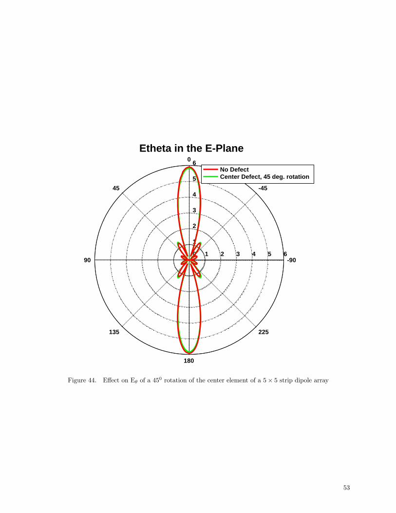
-90

-45

0

45

90

135

180

225

0

1

1

2

2

3

3

4

4

5

5

6

6

No DefectCenter Defect, 45 deg. rotation

Etheta in the E-Plane

Figure 44. Effect on Eθ of a 450 rotation of the center element of a 5× 5 strip dipole array

53

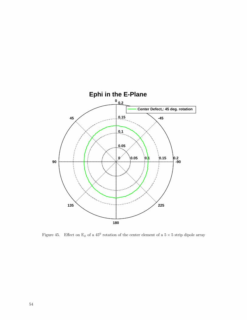
-90

-45

0

45

90

135

180

225

0

0.05

0.05

0.1

0.1

0.15

0.15

0.2

0.2

Center Defect,: 45 deg. rotation

Ephi in the E-Plane

Figure 45. Effect on Eφ of a 450 rotation of the center element of a 5× 5 strip dipole array

54

Input Input Descriptor

4 number of vertices of the array0.0 0.0 0.0 The coordinates of the vertices bounding the array, vertex 12.5 0.0 0.0 vertex 22.5 2.5 0.0 vertex 30.0 2.5 0.0 vertex 40.5 0.0 0.0 Lattice vector 1 describing periodicity in xy plane0.0 0.5 0.0 Lattice vector 2 describing periodicity in xy plane5 5 1 The number of interpolation points to use in the x,y,z direction.1 Flag - 1=use GIFFT, 0 =use block Toep.0 Preconditioner type - 0 = block diag 1= all near -1 = none.

0 ArrayFull3DFlag. 0 = no FFT in z. 1 = FFT in z.0 ArraySameExciteFlag. If 1, all right hand sides will be identical.0 ArrayPhasedFlag. 0=no phasing added, 1=linear phasing added to RHS0.0 0.0 The scan angle in theta and phi. This is ignored if ArrayPhasedFlag is 01 FastNearFlag. 1 = if using GIFFT, 0 = never use FFT for near field.0 ArrayPortAnalysisFlag2 Number of types of array elements in the array10 Number of meshing elements in first array element10 Number of meshing elements in second array element

1 Background element - this is the predominant element in the array.1 Number of array elements which are different from the background element (defect)13 2 Indices of the defect element and array element type they are

Table C. Array input file for a 5X5 array with center defect element.

4 The Seam Problem

The most general type of seam is shown in Figure 46 where the period (b) is maintained in the bydirection, but both shape of the unit cell and the period (a) is changed in the bx direction as we cross theseam. Again we use the three dots to denote the fact that the periodic structure is not truncated and weare studying only the scattering of the seam. We begin by studying the simplest seam imaginable thatretains the features of the general seam. This simple seam is made of two semi-infinite arrays of strips thatchange periodicity and strip width crossing the seam. We use this simple problem to understand how thefringe current magnitude compares to the magnitude of other currents in the vicinity of the seam. We thenformulate the 3D seam shown in Figure 46 and find that we need to first obtain a Green’s function for a 1darray of point sources. We go on to examine some useful approximations that we can exploit and finishwith using GIFFT to solve one of the special seam configurations — changing the unit cell shape across theseam, but maintaining a constant periodicity.

4.1 Numerically Exact, 1D Seam Problem

Figure 47 shows a seam between two perfect electric conducting (PEC) strip arrays. The strip arrayin the x > 0 region has a periodicity of a0, a strip width of wa0 and extends to x = +∞. The strip arrayin the x < 0 region has a periodicity of a, a strip width of wa and extends to x = −∞. A plane wave,

55

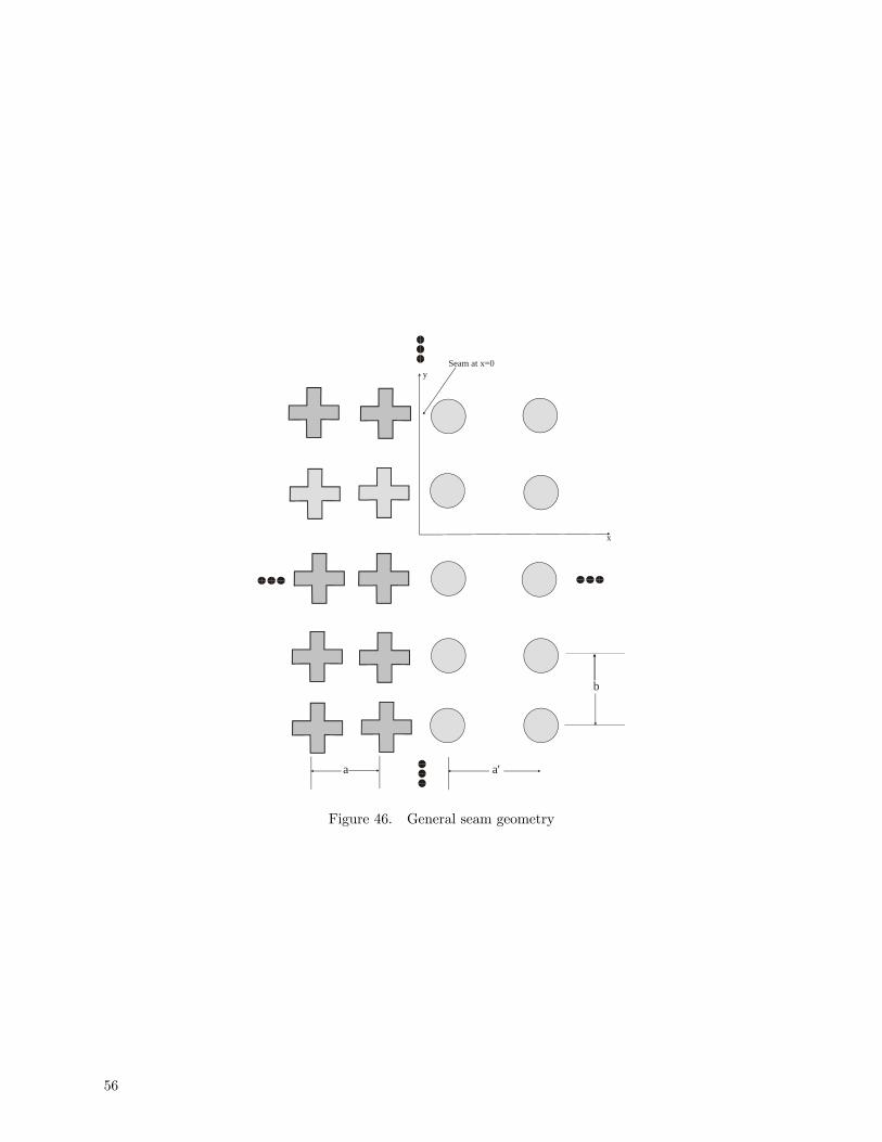
Seam at x=0

x

y

b

a a'

Figure 46. General seam geometry

56

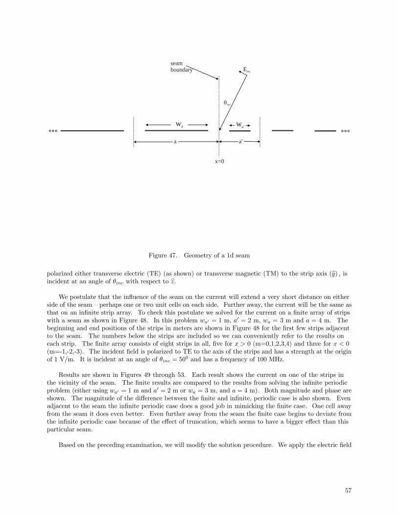
x=0

a'a

θinc

Einc

wa'wa

seamboundary

Figure 47. Geometry of a 1d seam

polarized either transverse electric (TE) (as shown) or transverse magnetic (TM) to the strip axis (by) , isincident at an angle of θinc with respect to bz.

We postulate that the influence of the seam on the current will extend a very short distance on eitherside of the seam — perhaps one or two unit cells on each side. Further away, the current will be the same asthat on an infinite strip array. To check this postulate we solved for the current on a finite array of stripswith a seam as shown in Figure 48. In this problem wa0 = 1 m, a0 = 2 m, wa = 3 m and a = 4 m. Thebeginning and end positions of the strips in meters are shown in Figure 48 for the first few strips adjacentto the seam. The numbers below the strips are included so we can conveniently refer to the results oneach strip. The finite array consists of eight strips in all, five for x > 0 (m=0,1,2,3,4) and three for x < 0(m=-1,-2,-3). The incident field is polarized to TE to the axis of the strips and has a strength at the originof 1 V/m. It is incident at an angle of θinc = 500 and has a frequency of 100 MHz.

Results are shown in Figures 49 through 53. Each result shows the current on one of the strips inthe vicinity of the seam. The finite results are compared to the results from solving the infinite periodicproblem (either using wa0 = 1 m and a0 = 2 m or wa = 3 m, and a = 4 m). Both magnitude and phase areshown. The magnitude of the difference between the finite and infinite, periodic case is also shown. Evenadjacent to the seam the infinite periodic case does a good job in mimicking the finite case. One cell awayfrom the seam it does even better. Even further away from the seam the finite case begins to deviate fromthe infinite periodic case because of the effect of truncation, which seems to have a bigger effect than thisparticular seam.

Based on the preceding examination, we will modify the solution procedure. We apply the electric field

57

-1-2-3 0 1 2 3 40.5-0.5 1.5 2.5-3.5-4.5-8.5 -7.5-11.5 3.5 8.5 9.5

E=1V/m

500

Figure 48. Finite seam

0.0 0.2 0.4 0.6 0.8x

0.000

0.001

0.002

0.003

0.004

0.005

J_ph

ase

-50

0

50

100

150

J_m

ag

Unit Cell 0

J_mag differenceJ_mag periodicJ_phase periodicJ_mag seamJ_phase seam

F=100 MHz, Theta=500

Figure 49. Current on strip at the m=0 position

58

0.0 0.5 1.0 1.5 2.0 2.5x

0.000

0.002

0.004

0.006

0.008

J_ph

ase

-100

-50

0

50

100

150J_

mag

Unit Cell -1

J_mag differenceJ_mag periodicJ_phase periodicJ_mag seamJ_phase seam

F=100 MHz, Theta=500

Figure 50. Current on strip at the m=-1 position

0.0 0.2 0.4 0.6 0.8x

0.000

0.001

0.002

0.003

0.004

0.005

J_ph

ase

135

140

145

150

155

160

J_m

ag

Unit Cell 1

J_mag differenceJ_mag periodicJ_phase periodicJ_mag seamJ_phase seam

F=100 MHz, Theta=500

Figure 51. Current on strip at the m=+1 position

59

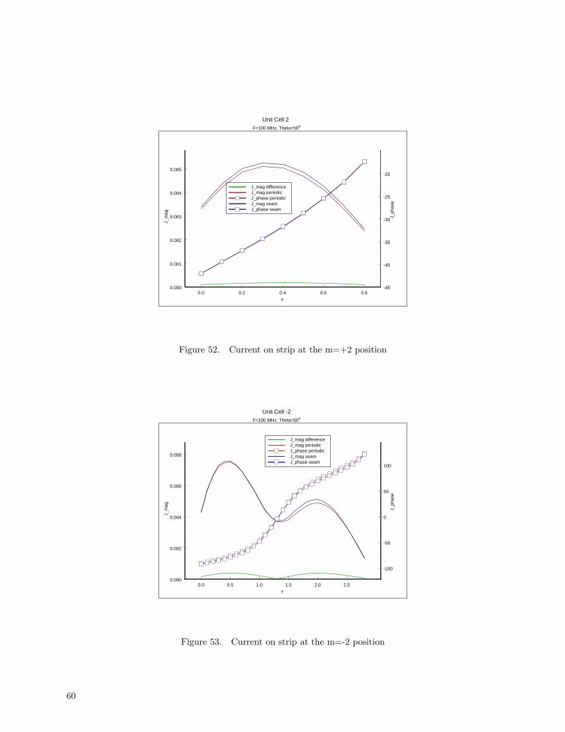
0.0 0.2 0.4 0.6 0.8x

0.000

0.001

0.002

0.003

0.004

0.005

J_ph

ase

-45

-40

-35

-30

-25

-20

J_m

ag

Unit Cell 2

J_mag differenceJ_mag periodicJ_phase periodicJ_mag seamJ_phase seam

F=100 MHz, Theta=500

Figure 52. Current on strip at the m=+2 position

0.0 0.5 1.0 1.5 2.0 2.5x

0.000

0.002

0.004

0.006

0.008

J_ph

ase

-100

-50

0

50

100

J_m

ag

Unit Cell -2

J_mag differenceJ_mag periodicJ_phase periodicJ_mag seamJ_phase seam

F=100 MHz, Theta=500

Figure 53. Current on strip at the m=-2 position

60

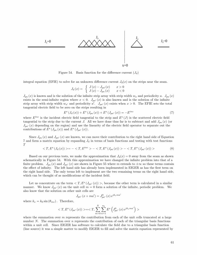
x=0

J ~0d

Jd Jd J ~0d

Figure 54. Basis function for the difference current (Jd)

integral equation (EFIE) to solve for an unknown difference current Jd(x) on the strips near the seam.

Jd (x) =

½J (x)− Jpa0(x) x > 0J (x)− Jpa (x) x < 0

Jpa (x) is known and is the solution of the infinite strip array with strip width wa and periodicity a. Jpa (x)exists in the semi-infinite region where x < 0. Jpa0 (x) is also known and is the solution of the infinitestrip array with strip width wa0 and periodicity a0. Jpa0 (x) exists when x > 0. The EFIE sets the totaltangential electric field to be zero on the strips resulting in

Es (Jd (x)) +Es (Jpa (x)) +Es (Jpa0 (x)) = −Einc (7)

where Einc is the incident electric field tangential to the strip and Es (J) is the scattered electric fieldtangential to the strip due to the current J. All we have done thus far is to subtract and add Jpa (x) (orJpa0 (x) depending on the region) and use the linearity of the electric field operator to separate out thecontributions of Es (Jpa (x)) and Es (Jpa0 (x)) .

Since Jpa (x) and Jpa0 (x) are known, we can move their contribution to the right hand side of Equation7 and form a matrix equation by expanding Jd in terms of basis functions and testing with test functionsT

< T,Es (Jd (x)) >= − < T,Einc > − < T,Es (Jpa (x)) > − < T,Es (Jpa0 (x)) > (8)

Based on our previous tests, we make the approximation that Jd(x) = 0 away from the seam as shownschematically in Figure 54. With this approximation we have changed the infinite problem into that of afinite problem. Jpa (x) and Jpa0 (x) are shown in Figure 55 where m extends to ±∞ so these terms containthe effect of infinity. The left hand side has already been implemented in EIGER as has the first term onthe right hand side. The only terms left to implement are the two remaining terms on the right hand side,which can be thought of as modifications of the incident field.

Let us concentrate on the term < T,Es (Jpa0 (x)) >, because the other term is calculated in a similarmanner. We know Jpa0 (x) on the unit cell m = 0 form a solution of the infinite, periodic problem. Wealso know that the solution on other unit cells are

Jpa0 (x+ma0) = J0pa0 (x) ejkxma0

where kx = k0 sin (θinc) . Therefore,

< T,Es (Jpa0 (x)) >=< T,NX

m=0

nbXn=1

Es³J0pa0 (x) e

jkxma0´>

where the summation over m represents the contribution from each of the unit cells truncated at a largenumber N. The summation over n represents the contribution of each of the triangular basis functionswithin a unit cell. Since EIGER has software to calculate the field due to a triangular basis function(line source) it was a simple matter to modify EIGER to fill and solve the matrix equation represented by

61

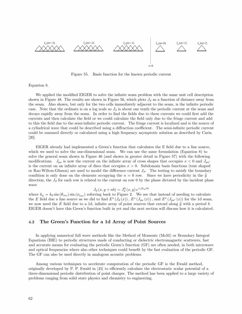
x=0

Jpa(m=-3) Jpa(m=-2) Jpa'(m=1)Jpa(m=-1) Jpa'(m=2)Jpa'(m=0)

Figure 55. Basis function for the known periodic current

Equation 8.

We applied the modified EIGER to solve the infinite seam problem with the same unit cell descriptionshown in Figure 48. The results are shown in Figure 56, which plots Jd as a function of distance away fromthe seam. Also shown, but only for the two cells immediately adjacent to the seam, is the infinite periodiccase. Note that the ordinate is on a log scale so Jd is about one tenth the periodic current at the seam anddecays rapidly away from the seam. In order to find the fields due to these currents we could first add thecurrents and then calculate the field or we could calculate the field only due to the fringe current and addto this the field due to the semi-infinite periodic current. The fringe current is localized and is the source ofa cylindrical wave that could be described using a diffraction coefficient. The semi-infinite periodic currentcould be summed directly or calculated using a high frequency asymptotic solution as described by Carin[20].

EIGER already had implemented a Green’s function that calculates the E field due to a line source,which we used to solve the one-dimensional seam. We can use the same formulation (Equation 8) tosolve the general seam shown in Figure 46 (and shown in greater detail in Figure 57) with the followingmodifications. Jpa is now the current on the infinite array of cross shapes that occupies x < 0 and Jpa0is the current on an infinite array of discs that occupies x > 0. Subdomain basis functions (tent shapedor Rao-Wilton-Glisson) are used to model the difference current Jd. The testing to satisfy the boundarycondition is only done on the elements occupying the n = 0 row. Since we have periodicity in the bydirection, the Jd for each row is related to the current on row 0 by the phase dictated by the incident planewave

Jd (x, y + nb) = J0d (x, y) e+jkynb

where ky = k0 sin (θinc) sin (φinc) referring back to Figure 2. We see that instead of needing to calculatethe E field due a line source as we did to find Es (Jd (x)) , E

s (Jpa (x)) , and Es (Jpa0 (x)) for the 1d seam,we now need the E field due to a 1d, infinite array of point sources that extend along by with a period b.EIGER doesn’t have this Green’s function built in yet and the next section will discuss how it is calculated.

4.2 The Green’s Function for a 1d Array of Point Sources

In applying numerical full wave methods like the Method of Moments (MoM) or Boundary IntegralEquations (BIE) to periodic structures made of conducting or dielectric electromagnetic scatterers, fastand accurate means for evaluating the periodic Green’s function (GF) are often needed, in both microwaveand optical frequencies where also other techniques could benefit by the fast evaluation of the periodic GF.The GF can also be used directly in analogous acoustic problems.

Among various techniques to accelerate computation of the periodic GF is the Ewald method,originally developed by P. P. Ewald in [45] to efficiently calculate the electrostatic scalar potential of athree-dimensional periodic distribution of point charges. The method has been applied to a large variety ofproblems ranging from solid state physics and chemistry to engineering.

62

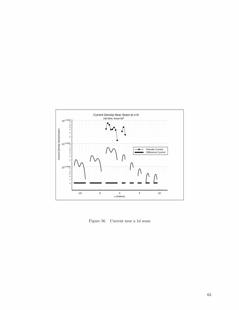
-10 -5 0 5 10x (meters)

10-4.0000

10-3.0000

10-2.0000

2

345679

2

345679

2

345679

Cur

rent

Den

sity

(Am

ps/m

eter

)

Periodic CurrentDifference Current

Current Density Near Seam at x=0100 MHz, theta=50o

Figure 56. Current near a 1d seam

63

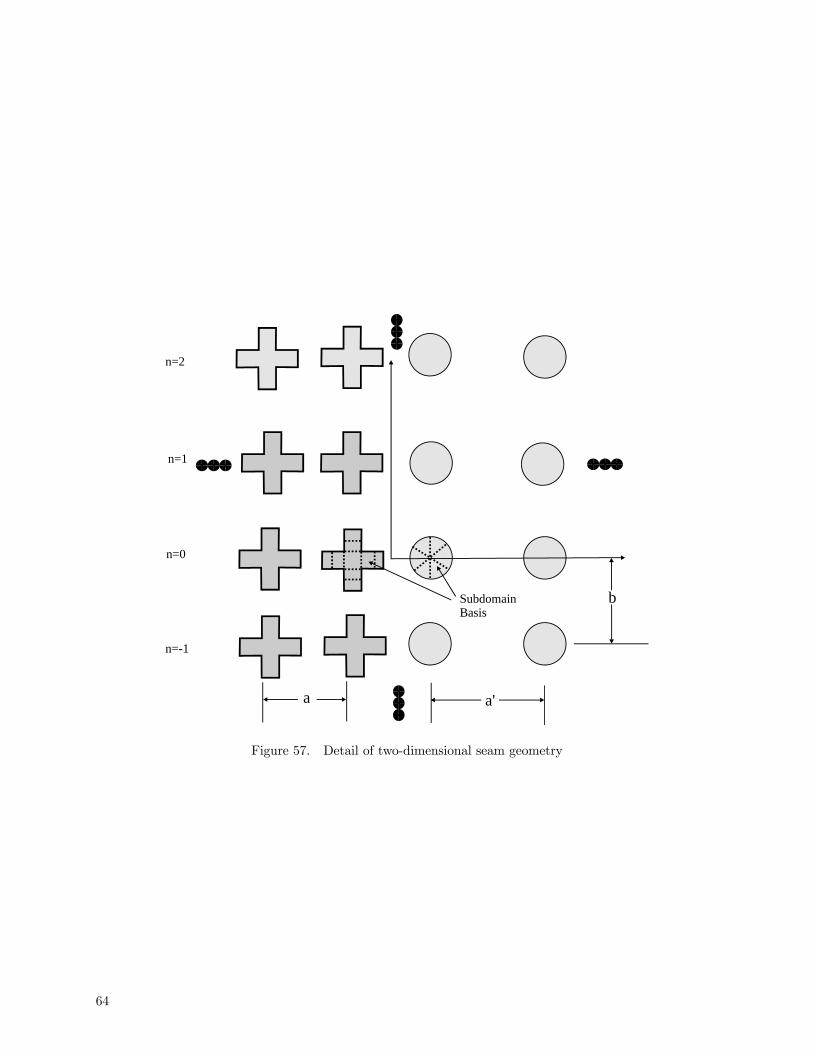
a a'

bSubdomainBasis

n=0

n=-1

n=1

n=2

Figure 57. Detail of two-dimensional seam geometry

64

In the following we describe the application of the method to the electrodynamic or acoustic problemssuch as the solution of the Helmholtz equation with periodic boundary conditions. We list here the Ewaldmethods that have been previously developed, and identify our own contribution.

Jordan et al. extended the Ewald method to the case of the free space GF for three dimensional (3D)problems with 2D periodicity (i.e., a planar array of point sources) in [46]. Its application in evaluatingGFs for multilayered media is treated in [47], [48], [49], [50]. The Ewald method is extended in [51],[52],[53] to 2D problems with 1D periodicity (i.e., a planar array of line sources). An analogous treatment ofthe GF for an array of line sources is reported in [54] where a more general view is also addressed, as wellas in [55] where a Schlömilch series that may arise in diffraction theory is efficiently evaluated. We alsopoint out that in [52] a comparison is made between various representations of the periodic GF concludingthat the Ewald method is one of the most advantageous. For a mathematical review of the Ewald methodin general, see [56]. For the case of a planar 2D-periodic array of point sources, the critical distance fromthe array plane beyond which the Ewald method is not advantageous compared to the standard spectralgrating lobe series is analyzed in [57].

The evaluation of the GF for a rectangular cavity using the Ewald method is reported in [58], and itsdyadic form in [59]. An application of the Ewald representation to hybrid methods involving a boundaryintegral equation and finite element method, for periodic structures, is given in [60]. In [61] the Ewaldmethod is combined with another very effective method to analyze scattering by periodically etched layeredconducting surfaces such as are commonly used for frequency selective surfaces.

Using the Ewald method, we accelerate for the first time the GF pertaining to a linear array of pointsources (i.e., a 3D problem with 1D periodicity.) The formula representations obtained in the abovementioned studies, i.e., the GF for geometries such as the 2D-periodic array of point sources [46], and the1D-periodic array of line sources [51],[52],[53],[54], cannot be applied to this new geometry. The standardpurely spectral sum representation for the GF cannot be used for this new particular configuration becauseit diverges when the observation point lies on the axis of the linear array, thus further proving the utility ofthe Ewald method, which exhibits a Gaussian convergence. A numerical analysis of the convergence rate isalso provided, supported by analytical considerations. As previously noted in [62], at high frequencies suchthat the wavelength is somewhat smaller than the period, computing the Ewald series using the optimalsplitting parameter E0 (see [46]) may yield inaccurate results due to the finiteness of machine precision.In [62] it is suggested that such numerical inaccuracies may be improved by increasing the value of thesplitting parameter E as frequency increases, but no guidelines for choosing the parameter are given.Here we present an algorithm for choosing the Ewald splitting parameter E that extends the efficiency ofthe method when the wavelength is somewhat smaller than the periodicity. The proposed algorithm isefficiently applied to periodic structures when the observation point is near the axis of the linear array ofpoint sources.

For several numerical methods such as MoM or BIE applied to periodic structures with period d alongz, it may be convenient to find the scalar potential radiated by an infinite linear array of point sourceslocated at r0n = ndz, where bold symbols define vector quantities, the caret () defines unit vectors, andn = 0,±1,±2, .... The point sources may be excited with a linear phase progression e−jkz0z, where kz0 isthe longitudinal wavenumber, that may originate by an impinging plane wave (impressed wavenumber) orby generators within each cell with a linear phase progression. An ejωt time dependence, with j =

√−1, isassumed and suppressed throughout this paper. If one adopts an e−iωt time dependence, with i =

√−1,all intermediate and final formula here derived apply as well after complex conjugation.

The GF for such a problem periodic along z, with period d, is given by the outgoing solution of theHelmholtz equation ∇2G(r, r0) + k2G(r, r0) = −δp(r0), where the periodic (along z) forcing term δp(r

0) iswritten as δp(r0) =

P∞n=0 δ(x

0)δ(y0)δ(z0 − nd)e−jkz0nd. The GF solution of the Helmholtz equation may be

65

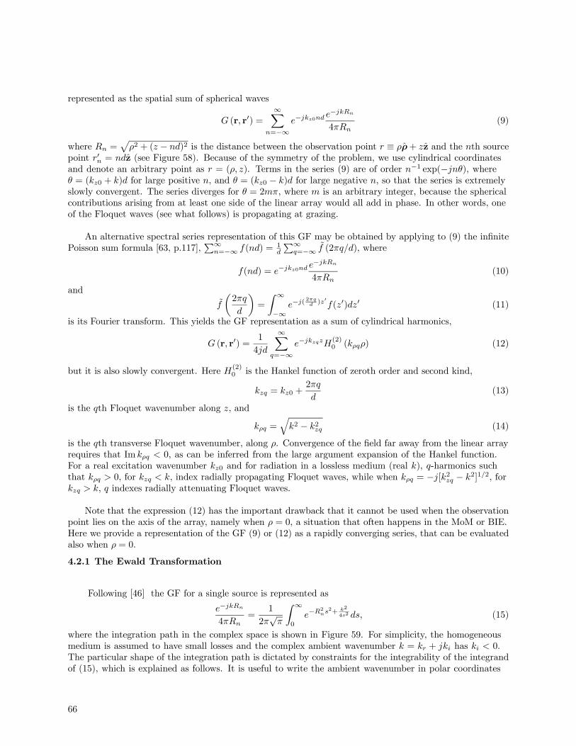
represented as the spatial sum of spherical waves

G (r, r0) =∞X

n=−∞e−jkz0nd

e−jkRn

4πRn(9)

where Rn =pρ2 + (z − nd)2 is the distance between the observation point r ≡ ρρ+ zz and the nth source

point r0n = ndz (see Figure 58). Because of the symmetry of the problem, we use cylindrical coordinatesand denote an arbitrary point as r = (ρ, z). Terms in the series (9) are of order n−1 exp(−jnθ), whereθ = (kz0 + k)d for large positive n, and θ = (kz0 − k)d for large negative n, so that the series is extremelyslowly convergent. The series diverges for θ = 2mπ, where m is an arbitrary integer, because the sphericalcontributions arising from at least one side of the linear array would all add in phase. In other words, oneof the Floquet waves (see what follows) is propagating at grazing.

An alternative spectral series representation of this GF may be obtained by applying to (9) the infinitePoisson sum formula [63, p.117],

P∞n=−∞ f(nd) = 1

d

P∞q=−∞ f (2πq/d), where

f(nd) = e−jkz0nde−jkRn

4πRn(10)

and

f

µ2πq

d

¶=

Z ∞−∞

e−j(2πqd )z0f(z0)dz0 (11)

is its Fourier transform. This yields the GF representation as a sum of cylindrical harmonics,

G (r, r0) =1

4jd

∞Xq=−∞

e−jkzqzH(2)0 (kρqρ) (12)

but it is also slowly convergent. Here H(2)0 is the Hankel function of zeroth order and second kind,

kzq = kz0 +2πq

d(13)

is the qth Floquet wavenumber along z, and

kρq =qk2 − k2zq (14)

is the qth transverse Floquet wavenumber, along ρ. Convergence of the field far away from the linear arrayrequires that Im kρq < 0, as can be inferred from the large argument expansion of the Hankel function.For a real excitation wavenumber kz0 and for radiation in a lossless medium (real k), q-harmonics suchthat kρq > 0, for kzq < k, index radially propagating Floquet waves, while when kρq = −j[k2zq − k2]1/2, forkzq > k, q indexes radially attenuating Floquet waves.

Note that the expression (12) has the important drawback that it cannot be used when the observationpoint lies on the axis of the array, namely when ρ = 0, a situation that often happens in the MoM or BIE.Here we provide a representation of the GF (9) or (12) as a rapidly converging series, that can be evaluatedalso when ρ = 0.

4.2.1 The Ewald Transformation

Following [46] the GF for a single source is represented as

e−jkRn

4πRn=

1

2π√π

Z ∞0

e−R2ns

2+ k2

4s2 ds, (15)

where the integration path in the complex space is shown in Figure 59. For simplicity, the homogeneousmedium is assumed to have small losses and the complex ambient wavenumber k = kr + jki has ki < 0.The particular shape of the integration path is dictated by constraints for the integrability of the integrandof (15), which is explained as follows. It is useful to write the ambient wavenumber in polar coordinates

66

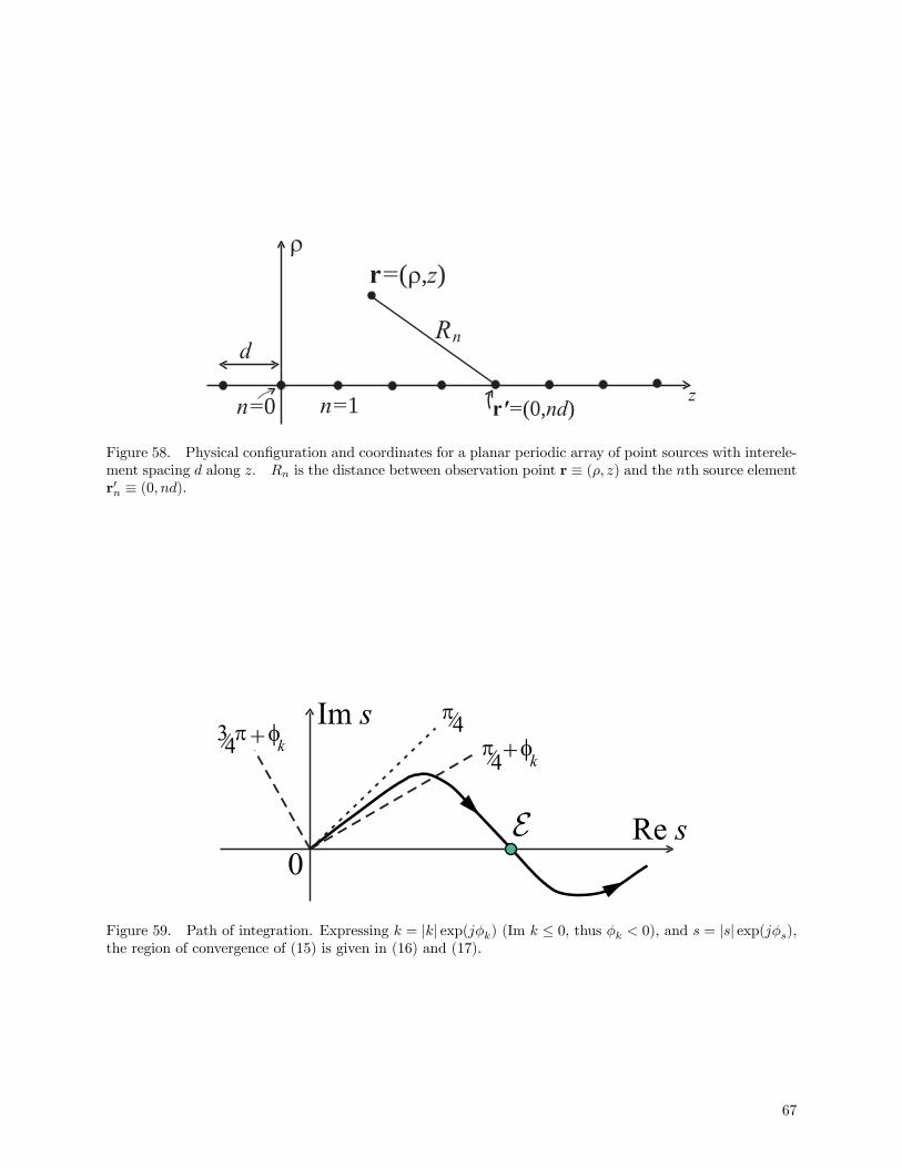
zr'= nd(0, )

Rn

d

n=0 n=1

r=( ),z

Figure 58. Physical configuration and coordinates for a planar periodic array of point sources with interele-ment spacing d along z. Rn is the distance between observation point r ≡ (ρ, z) and the nth source elementr0n ≡ (0, nd).

Im s

Re s

0

k

k

Figure 59. Path of integration. Expressing k = |k| exp(jφk) (Im k ≤ 0, thus φk < 0), and s = |s| exp(jφs),the region of convergence of (15) is given in (16) and (17).

67

k = |k|ejφk , with φk = arctan(ki/kr) < 0, and s = sr + jsi = |s| exp(jφs) with φs = arctan(si/sr). Indeed,convergence of (15) is ensured by requiring that Re[k2/s2] < 0 for s→ 0, and Re[R2ns

2] > 0 for s→∞, i.e.,3

4π + φk ≥ φs ≥

π

4+ φk, for s→ 0 (16)

π

4> φs > −

π

4, for s→∞ (17)

which are satisfied by the path in Figure 59. The Ewald method is obtained by splitting the integral in (15)

into two parts,R∞0=³R E

0+R∞E´, which also determines the splitting

G (r, r0) = Gspectral (r, r0) +Gspatial (r, r

0) (18)

Gspectral (r, r0) =

1

2π√π

∞Xn=−∞

e−jkz0ndZ E

0

e−Rns2+ k2

4s2 ds (19)

Gspatial (r, r0) =

1

2π√π

∞Xn=−∞

e−jkz0ndZ ∞E

e−R2ns

2+ k2

4s2 ds. (20)

The spatial term Gspatial exhibits a Gaussian exponential convergence in n as can be inferred by noticingthat Re(s) > E on the complex integration path and for large n the integral in (20) behaves like1√π

R∞E e−n

2d2s2ds = (2nd)−1erfc(nEd), where

erfc(z) =2√π

Z ∞z

e−t2

dt (21)

is the complementary error function. For large argument it is approximated by erfc(z) ∼ e−z2

/(√πz),

which highlights the Gaussian n-convergence of (20). The spectral term (19) instead is slowly convergingas 1/n, since the original series (9) converges as 1/n, and requires the use of the Poisson transformation toaccelerate its convergence.

4.2.2 The Spectral Part of the Green’s function

To accelerate the spectral part (19) of the GF in (18) we first apply the Poisson’s sum formula, (cf.,discussion before (10)), with

f(nd) = e−jkz0ndZ E

0

e−[ρ2+(z−nd)2]s2+ k2

4s2 ds. (22)

The evaluation of the Fourier transform f (2πq/d), defined in (11), is carried out by first changing the orderof integration, which is possible since Re(s2) > 0 on the integration path shown in Figure 59. More detailson these mathematical steps are in [53, Section IV-A] where an analogous problem is treated. Then, thechange of variable (z0, s)→ (u, s), with u = (z− z0)s, after evaluation of the resulting u-integral, leads to

f

µ2πq

d

¶=√πe−jkzqz

Z E

0

e−ρ2s2+

k2ρq

4s2ds

s. (23)

Note that Re(k2ρq), with k2ρq = k2 − k2zq, is negative for large q resulting in evanescent Floquet modes,hence the above integral is exponentially converging for large q. Let u = 1

4s2 , withdss = −12 duu , so that the

above integral is rewritten as

f

µ2πq

d

¶=

√π

2e−jkzqz

Z ∞1

4E2

e−ρ2

4u+k2ρqu

du

u(24)

where the mapped integration path goes to infinity in the region between π2 and

3π2 for real kρq (propagating

modes), and in the region between −π2 and

π2 for imaginary kρq (evanescent modes). The same argument

applies when small ambient losses are present, while a deeper analysis is required for complex propagation

68

constants kzq.

Next, following a procedure analogous to [51], [53, Section IV-B], we utilize the Taylor expansione−ρ

2/(4u) =P∞

p=0(−1)p(ρ/2)2p/(p!up). After using the change of variable w = 4E2u, an integration of theseries term by term leads to

f

µ2πq

d

¶=

√π

2e−jkzqz

∞Xp=0

(−1)pp!

(ρE)2pEp+1(−k2ρq4E2 ) (25)

in which Ep(x) is the pth order exponential integral defined by [64, p. 228]

E1(x) =

Z ∞x

e−t

tpdt, |argx| < π, (26)

and by the recurrence relation [64, p. 229]

Ep+1(x) =1

p[e−x − xEp(x)], p = 1, 2, 3, .... (27)

The path of integration in (26) should exclude the origin and not cross the negative real axis [64,p. 229]. For evanescent waves, −k2ρq > 0 and one can also use the definition Ep(x) =

R∞1

e−xt t−pdt, validfor Rex > 0. Substituting (25) into the Poisson transform of the original expression (19) leads to

Gspectral (r, r0) =

1

4πd

∞Xq=−∞

e−jkzqz∞Xp=0

(−1)pp!

(ρE)2pEp+1(−k2ρq4E2 ). (28)

The exponential integral E1(x) may be evaluated using the algorithm of [64, Section 5.1.53] for 0 ≤ x ≤ 1,or [64, Section 5.1.56]) for 1 ≤ x < ∞. Though a double series, expression (28) is rapidly convergent.Indeed, only a handful of q terms and around ten p terms are necessary to reach a good accuracy, as shownin Section 4.2.8.

The exponential integral (26) has a branch cut along the negative real axis. Note that in absence ofambient losses, and for a real phasing wavenumber kz0 along the array, all propagating Floquet waves havek2ρq = k2 − k2zq > 0 and thus the argument of the exponential integral in (28) is negative real, resulting inan ambiguous branch condition.

To resolve the ambiguity we imagine small ambient losses such that Im(−k2ρq) > 0 and therefore thebranch can be chosen automatically and one can use (26) directly. Though the assumption of losses isuseful for the branch determination, in lossless media one may prefer to evaluate Ep+1(x) obtained usingthe formula E1(−x+ j0+) = −Ei(x)− jπ, [64, p. 228], with

Ei(x) = −PZ ∞−x

e−t

tdt, x > 0, (29)

where P denotes principal-value integration. For small argument the exponential integral Ei can beevaluated as Ei(x) = γ + lnx +

P∞n=1 x

n/(nn!), for x > 0, where γ ≈ 0.57721566 is the Euler constant.Note that once E1(−x+ j0+) is obtained, Ep+1(−x+ j0+) follows from (27).

4.2.3 The Spatial Part of the Green’s function

The spatial part of the GF in (20) already exhibits Gaussian convergence; here we reexpress it in termsof complementary error functions. Consider a generic n-term of the spatial series in (20)

In =

Z ∞E

e−R2ns

2+ k2

4s2 ds = ejkRnZ ∞E

e−[Rns+jk2s ]

2

ds. (30)

With the change of variable of u = Rns+ jk/(2s), or s = (u+pu2 − j2kRn)/(2Rn), (30) is transformed

69

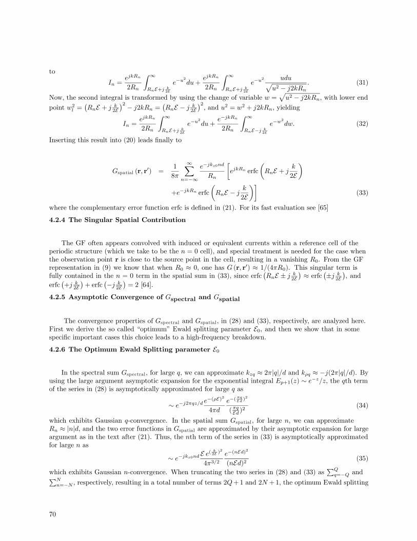
to

In =ejkRn

2Rn

Z ∞RnE+j k

2E

e−u2

du+ejkRn

2Rn

Z ∞RnE+j k

2E

e−u2 udup

u2 − j2kRn

. (31)

Now, the second integral is transformed by using the change of variable w =pu2 − j2kRn, with lower end

point w2l =¡RnE + j k

2E¢2 − j2kRn =

¡RnE − j k

2E¢2, and u2 = w2 + j2kRn, yielding

In =ejkRn

2Rn

Z ∞RnE+j k

2E

e−u2

du+e−jkRn

2Rn

Z ∞RnE−j k

2E

e−w2

dw. (32)

Inserting this result into (20) leads finally to

Gspatial (r, r0) =

1

8π

∞Xn=−∞

e−jkz0nd

Rn

∙ejkRn erfc

µRnE + j

k

2E¶

+e−jkRn erfcµRnE − j

k

2E¶¸

(33)

where the complementary error function erfc is defined in (21). For its fast evaluation see [65]

4.2.4 The Singular Spatial Contribution

The GF often appears convolved with induced or equivalent currents within a reference cell of theperiodic structure (which we take to be the n = 0 cell), and special treatment is needed for the case whenthe observation point r is close to the source point in the cell, resulting in a vanishing R0. From the GFrepresentation in (9) we know that when R0 ≈ 0, one has G (r, r0) ≈ 1/(4πR0). This singular term isfully contained in the n = 0 term in the spatial sum in (33), since erfc

¡RnE ± j k

2E¢ ≈ erfc ¡±j k

2E¢, and

erfc¡+j k

2E¢+ erfc

¡−j k2E¢= 2 [64].

4.2.5 Asymptotic Convergence of Gspectral and Gspatial

The convergence properties of Gspectral and Gspatial , in (28) and (33), respectively, are analyzed here.First we derive the so called “optimum” Ewald splitting parameter E0, and then we show that in somespecific important cases this choice leads to a high-frequency breakdown.

4.2.6 The Optimum Ewald Splitting parameter E0

In the spectral sum Gspectral , for large q, we can approximate kzq ≈ 2π|q|/d and kρq ≈ −j(2π|q|/d). Byusing the large argument asymptotic expansion for the exponential integral Ep+1(z) ∼ e−z/z, the qth termof the series in (28) is asymptotically approximated for large q as

∼ e−j2πqz/de−(ρE)

2

4πd

e−(πqEd )

2

(πqEd)2

(34)

which exhibits Gaussian q-convergence. In the spatial sum Gspatial , for large n, we can approximateRn ≈ |n|d, and the two error functions in Gspatial are approximated by their asymptotic expansion for largeargument as in the text after (21). Thus, the nth term of the series in (33) is asymptotically approximatedfor large n as

∼ e−jkz0ndE e( k2E )24π3/2

e−(nEd)2

(nEd)2 (35)

which exhibits Gaussian n-convergence. When truncating the two series in (28) and (33) asPQ

q=−Q andPNn=−N , respectively, resulting in a total number of terms 2Q+1 and 2N +1, the optimum Ewald splitting

70

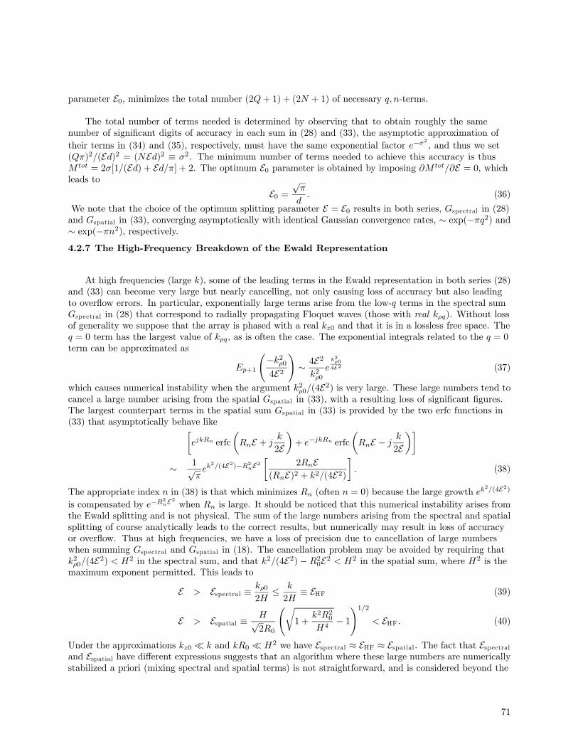
parameter E0, minimizes the total number (2Q+ 1) + (2N + 1) of necessary q, n-terms.

The total number of terms needed is determined by observing that to obtain roughly the samenumber of significant digits of accuracy in each sum in (28) and (33), the asymptotic approximation oftheir terms in (34) and (35), respectively, must have the same exponential factor e−σ

2

, and thus we set(Qπ)2/(Ed)2 = (NEd)2 ≡ σ2. The minimum number of terms needed to achieve this accuracy is thusM tot = 2σ[1/(Ed) + Ed/π] + 2. The optimum E0 parameter is obtained by imposing ∂M tot/∂E = 0, whichleads to

E0 =√π

d. (36)

We note that the choice of the optimum splitting parameter E = E0 results in both series, Gspectral in (28)and Gspatial in (33), converging asymptotically with identical Gaussian convergence rates, ∼ exp(−πq2) and∼ exp(−πn2), respectively.4.2.7 The High-Frequency Breakdown of the Ewald Representation

At high frequencies (large k), some of the leading terms in the Ewald representation in both series (28)and (33) can become very large but nearly cancelling, not only causing loss of accuracy but also leadingto overflow errors. In particular, exponentially large terms arise from the low-q terms in the spectral sumGspectral in (28) that correspond to radially propagating Floquet waves (those with real kρq). Without lossof generality we suppose that the array is phased with a real kz0 and that it is in a lossless free space. Theq = 0 term has the largest value of kρq, as is often the case. The exponential integrals related to the q = 0term can be approximated as

Ep+1

Ã−k2ρ04E2

!∼ 4E

2

k2ρ0ek2ρ0

4E2 (37)

which causes numerical instability when the argument k2ρ0/(4E2) is very large. These large numbers tend tocancel a large number arising from the spatial Gspatial in (33), with a resulting loss of significant figures.The largest counterpart terms in the spatial sum Gspatial in (33) is provided by the two erfc functions in(33) that asymptotically behave like∙

ejkRn erfc

µRnE + j

k

2E¶+ e−jkRn erfc

µRnE − j

k

2E¶¸

∼ 1√πek

2/(4E2)−R2nE2

∙2RnE

(RnE)2 + k2/(4E2)¸. (38)

The appropriate index n in (38) is that which minimizes Rn (often n = 0) because the large growth ek2/(4E2)

is compensated by e−R2nE2 when Rn is large. It should be noticed that this numerical instability arises from

the Ewald splitting and is not physical. The sum of the large numbers arising from the spectral and spatialsplitting of course analytically leads to the correct results, but numerically may result in loss of accuracyor overflow. Thus at high frequencies, we have a loss of precision due to cancellation of large numberswhen summing Gspectral and Gspatial in (18). The cancellation problem may be avoided by requiring thatk2ρ0/(4E2) < H2 in the spectral sum, and that k2/(4E2)− R20E2 < H2 in the spatial sum, where H2 is themaximum exponent permitted. This leads to

E > Espectral ≡ kρ02H≤ k

2H≡ EHF (39)

E > Espatial ≡ H√2R0

Ãr1 +

k2R20H4

− 1!1/2

< EHF . (40)

Under the approximations kz0 ¿ k and kR0 ¿ H2 we have Espectral ≈ EHF ≈ Espatial . The fact that Espectraland Espatial have different expressions suggests that an algorithm where these large numbers are numericallystabilized a priori (mixing spectral and spatial terms) is not straightforward, and is considered beyond the

71

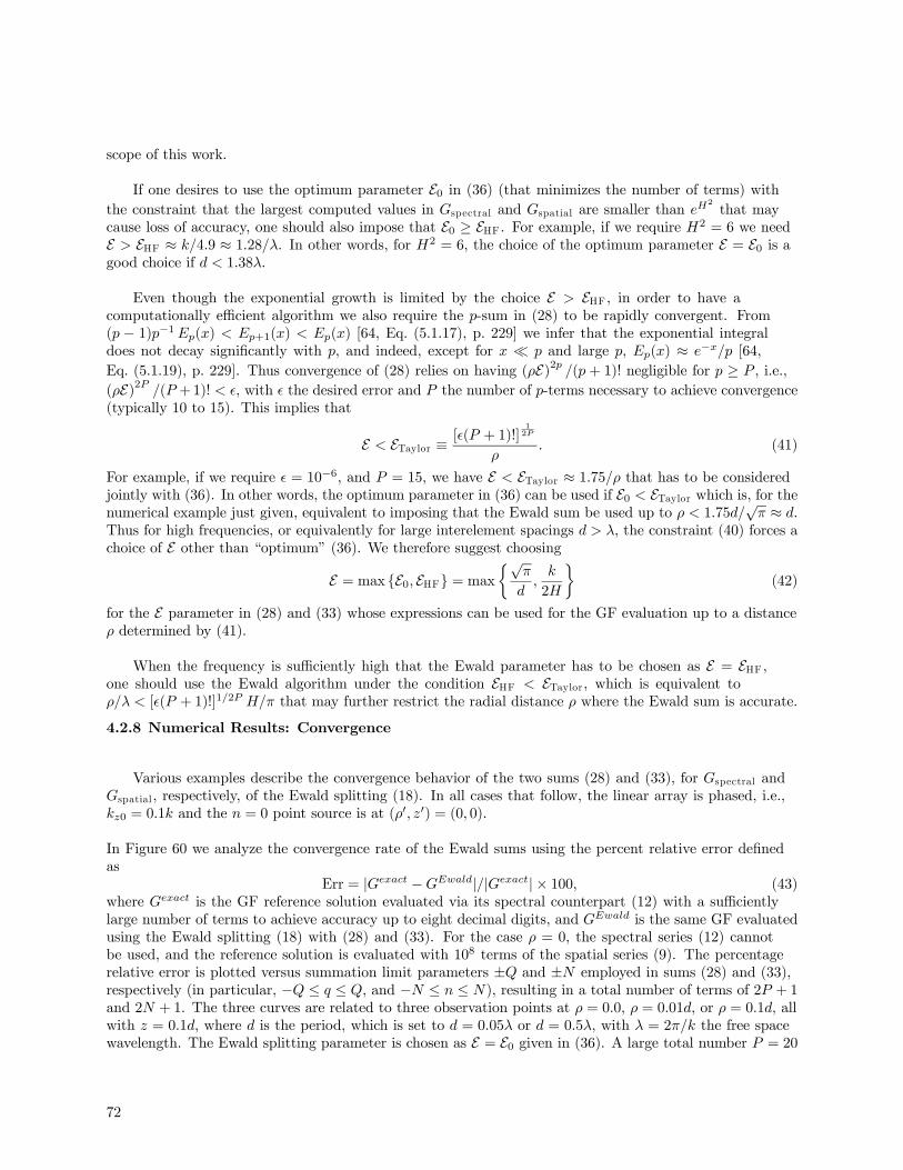
scope of this work.

If one desires to use the optimum parameter E0 in (36) (that minimizes the number of terms) withthe constraint that the largest computed values in Gspectral and Gspatial are smaller than eH

2

that maycause loss of accuracy, one should also impose that E0 ≥ EHF. For example, if we require H2 = 6 we needE > EHF ≈ k/4.9 ≈ 1.28/λ. In other words, for H2 = 6, the choice of the optimum parameter E = E0 is agood choice if d < 1.38λ.

Even though the exponential growth is limited by the choice E > EHF, in order to have acomputationally efficient algorithm we also require the p-sum in (28) to be rapidly convergent. From(p − 1)p−1Ep(x) < Ep+1(x) < Ep(x) [64, Eq. (5.1.17), p. 229] we infer that the exponential integraldoes not decay significantly with p, and indeed, except for x ¿ p and large p, Ep(x) ≈ e−x/p [64,Eq. (5.1.19), p. 229]. Thus convergence of (28) relies on having (ρE)2p /(p + 1)! negligible for p ≥ P , i.e.,(ρE)2P /(P +1)! < , with the desired error and P the number of p-terms necessary to achieve convergence(typically 10 to 15). This implies that

E < ETaylor ≡ [ (P + 1)!]12P

ρ. (41)

For example, if we require = 10−6, and P = 15, we have E < ETaylor ≈ 1.75/ρ that has to be consideredjointly with (36). In other words, the optimum parameter in (36) can be used if E0 < ETaylor which is, for thenumerical example just given, equivalent to imposing that the Ewald sum be used up to ρ < 1.75d/

√π ≈ d.

Thus for high frequencies, or equivalently for large interelement spacings d > λ, the constraint (40) forces achoice of E other than “optimum” (36). We therefore suggest choosing

E = max E0, EHF = max½√

π

d,k

2H

¾(42)

for the E parameter in (28) and (33) whose expressions can be used for the GF evaluation up to a distanceρ determined by (41).

When the frequency is sufficiently high that the Ewald parameter has to be chosen as E = EHF,one should use the Ewald algorithm under the condition EHF < ETaylor, which is equivalent toρ/λ < [ (P + 1)!]1/2P H/π that may further restrict the radial distance ρ where the Ewald sum is accurate.

4.2.8 Numerical Results: Convergence

Various examples describe the convergence behavior of the two sums (28) and (33), for Gspectral andGspatial , respectively, of the Ewald splitting (18). In all cases that follow, the linear array is phased, i.e.,kz0 = 0.1k and the n = 0 point source is at (ρ0, z0) = (0, 0).

In Figure 60 we analyze the convergence rate of the Ewald sums using the percent relative error definedas

Err = |Gexact −GEwald|/|Gexact| × 100, (43)where Gexact is the GF reference solution evaluated via its spectral counterpart (12) with a sufficientlylarge number of terms to achieve accuracy up to eight decimal digits, and GEwald is the same GF evaluatedusing the Ewald splitting (18) with (28) and (33). For the case ρ = 0, the spectral series (12) cannotbe used, and the reference solution is evaluated with 108 terms of the spatial series (9). The percentagerelative error is plotted versus summation limit parameters ±Q and ±N employed in sums (28) and (33),respectively (in particular, −Q ≤ q ≤ Q, and −N ≤ n ≤ N), resulting in a total number of terms of 2P + 1and 2N + 1. The three curves are related to three observation points at ρ = 0.0, ρ = 0.01d, or ρ = 0.1d, allwith z = 0.1d, where d is the period, which is set to d = 0.05λ or d = 0.5λ, with λ = 2π/k the free spacewavelength. The Ewald splitting parameter is chosen as E = E0 given in (36). A large total number P = 20

72

( )b

1.E-05

1.E-04

1.E-03

1.E-02

1.E-01

1.E+00

1.E+01

0 1 2 3N (Q=N)

Rela

tive

Err

or

(%) x=0

x=0.01d

x=0.1d

1.E-05

1.E-04

1.E-03

1.E-02

1.E-01

1.E+00

1.E+01

0 1 2 3N (Q=N)

Rela

tive

Err

or

(%) x=0

x=0.01d

x=0.1d

( )a

d=0.05 d=0.5

Figure 60. Convergence of the Ewald sums in (18) with (28) and (33) evaluated at three observation pointswith ρ = 0.0, 0.01d, 0.1d and z = 0.1d. Percentage relative error versus number of terms N (Q = N) in thesums for two cases with period d = 0.05λ and d = 0.5λ. Curves for ρ = 0 and ρ = 0.01d are superimposed.

of p-terms in (28) has been used because we emphasize here convergence issues related only to N and Q.

Figure 60 shows that just a few terms, Q = 1 and N = 1, provide six digits of accuracy. The relativeerror cannot be further decreased by augmenting the number of terms Q,N in Gspectral, Gspatial becauseof the accuracy limits of the numerical subroutines that evaluate the error functions in Gspatial and theexponential integral E1(x) in Gspectral (see [65] for erfc(x), and [64, Secs. 5.1.53, 5.1.56] for E1(x)).Note that in both cases in Figure 60 the period d is smaller than the wavelength, and that acceptingexponential factors of the order of eH

2

with H2 = 9.6, i.e., with roughly six digits of accuracy, impliesEHF = k/6.2 = 1.01/λ. According to (36), for d = 0.05λ and d = 0.5λ, the optimal Ewald parameter isE0 = 35.4/λ and E0 = 3.54/λ, respectively, and thus in both cases we have E0 > EHF justifying the use ofthe optimum Ewald parameter E0.

To gain an idea of the exceptional convergence rate of the Ewald representation, independent of theaccuracy error of the evaluation of the special functions E1(x) and erfc(x), Figure 61 shows the rate ofconvergence of the two individual series Gspectral and Gspatial in (28) and (33), respectively, evaluated atthe location r = (ρ, z) = (0.1, 0.1)d ( we have checked that the case with z = 0.1d would lead to analogousresults). The relative error is defined as

Err spectral, spatial =|GEwald,exact

spectral, spatial −GEwald,P,Mspectral, spatial|

|GEwald,exactspectral, spatial|

× 100, (44)

where GEwald,exactspectral, spatial is either Gspectral or Gspatial evaluated with a sufficient number of terms to achieve

high numerical accuracy. The error is plotted versus the summation limit parameters ±Q and ±N employedin the sums in Gspectral and Gspatial , respectively. The array is the same as that in Figure 60(b), i.e.,d = 0.5λ. The convergence rate is shown for three different choices of the Ewald splitting parameter E .Note that the optimum parameter E = E0 leads to the same convergence rate for both Gspectral and inGspatial (Figure 61(b)), and the two series need the same number of terms to achieve the same accuracy.It is remarkable that so few terms are required to achieve high accuracy. For E < E0 the spectral sumin Gspectral converges more rapidly than the sum in Gspatial . Vice versa for E > E0, as predicted by theasymptotic expansion of the spectral and spatial sums in (34) and (35), respectively.

To determine the number P of necessary p-terms used in the Taylor expansion in (25), the percentage

73

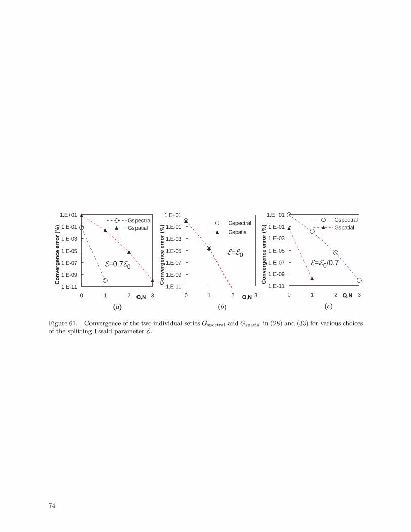
1.E-11

1.E-09

1.E-07

1.E-05

1.E-03

1.E-01

1.E+01

0 1 2 3Q,N

Co

nverg

en

ce

err

or

(%)

Gspectral

Gspatial

1.E-11

1.E-09

1.E-07

1.E-05

1.E-03

1.E-01

1.E+01

0 1 2 3Q,N

Co

nverg

en

ce

err

or

(%)

Gspectral

Gspatial

1.E-11

1.E-09

1.E-07

1.E-05

1.E-03

1.E-01

1.E+01

0 1 2 3Q,N

Co

nverg

en

ce

err

or

(%) Gspectral

Gspatial

( )a ( )b ( )c

= 00.7

= 0

= 0/0.7

( )a

Figure 61. Convergence of the two individual series Gspectral and Gspatial in (28) and (33) for various choicesof the splitting Ewald parameter E.

74

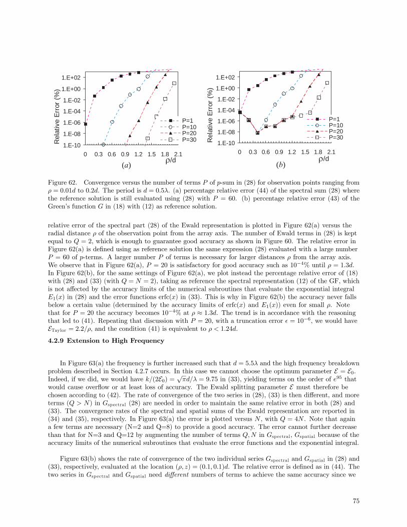
1.E-10

1.E-08

1.E-06

1.E-04

1.E-02

1.E+00

1.E+02

0 0.3 0.6 0.9 1.2 1.5 1.8 2.1x /d

Rela

tive

Err

or

(%)

P=1P=10P=20P=30

1.E-10

1.E-08

1.E-06

1.E-04

1.E-02

1.E+00

1.E+02

0 0.3 0.6 0.9 1.2 1.5 1.8 2.1x /d

Rela

tive

Err

or

(%)

P=1P=10P=20P=30

( )b( )a

Figure 62. Convergence versus the number of terms P of p-sum in (28) for observation points ranging fromρ = 0.01d to 0.2d. The period is d = 0.5λ. (a) percentage relative error (44) of the spectral sum (28) wherethe reference solution is still evaluated using (28) with P = 60. (b) percentage relative error (43) of theGreen’s function G in (18) with (12) as reference solution.

relative error of the spectral part (28) of the Ewald representation is plotted in Figure 62(a) versus theradial distance ρ of the observation point from the array axis. The number of Ewald terms in (28) is keptequal to Q = 2, which is enough to guarantee good accuracy as shown in Figure 60. The relative error inFigure 62(a) is defined using as reference solution the same expression (28) evaluated with a large numberP = 60 of p-terms. A larger number P of terms is necessary for larger distances ρ from the array axis.We observe that in Figure 62(a), P = 20 is satisfactory for good accuracy such as 10−4% until ρ = 1.3d.In Figure 62(b), for the same settings of Figure 62(a), we plot instead the percentage relative error of (18)with (28) and (33) (with Q = N = 2), taking as reference the spectral representation (12) of the GF, whichis not affected by the accuracy limits of the numerical subroutines that evaluate the exponential integralE1(x) in (28) and the error functions erfc(x) in (33). This is why in Figure 62(b) the accuracy never fallsbelow a certain value (determined by the accuracy limits of erfc(x) and E1(x)) even for small ρ. Notethat for P = 20 the accuracy becomes 10−4% at ρ ≈ 1.3d. The trend is in accordance with the reasoningthat led to (41). Repeating that discussion with P = 20, with a truncation error = 10−6, we would haveETaylor = 2.2/ρ, and the condition (41) is equivalent to ρ < 1.24d.4.2.9 Extension to High Frequency

In Figure 63(a) the frequency is further increased such that d = 5.5λ and the high frequency breakdownproblem described in Section 4.2.7 occurs. In this case we cannot choose the optimum parameter E = E0.Indeed, if we did, we would have k/(2E0) =

√πd/λ = 9.75 in (33), yielding terms on the order of e95 that

would cause overflow or at least loss of accuracy. The Ewald splitting parameter E must therefore bechosen according to (42). The rate of convergence of the two series in (28), (33) is then different, and moreterms (Q > N) in Gspectral (28) are needed in order to maintain the same relative error in both (28) and(33). The convergence rates of the spectral and spatial sums of the Ewald representation are reported in(34) and (35), respectively. In Figure 63(a) the error is plotted versus N , with Q = 4N . Note that againa few terms are necessary (N=2 and Q=8) to provide a good accuracy. The error cannot further decreasethan that for N=3 and Q=12 by augmenting the number of terms Q,N in Gspectral , Gspatial because of theaccuracy limits of the numerical subroutines that evaluate the error functions and the exponential integral.

Figure 63(b) shows the rate of convergence of the two individual series Gspectral and Gspatial in (28) and(33), respectively, evaluated at the location (ρ, z) = (0.1, 0.1)d. The relative error is defined as in (44). Thetwo series in Gspectral and Gspatial need different numbers of terms to achieve the same accuracy since we

75

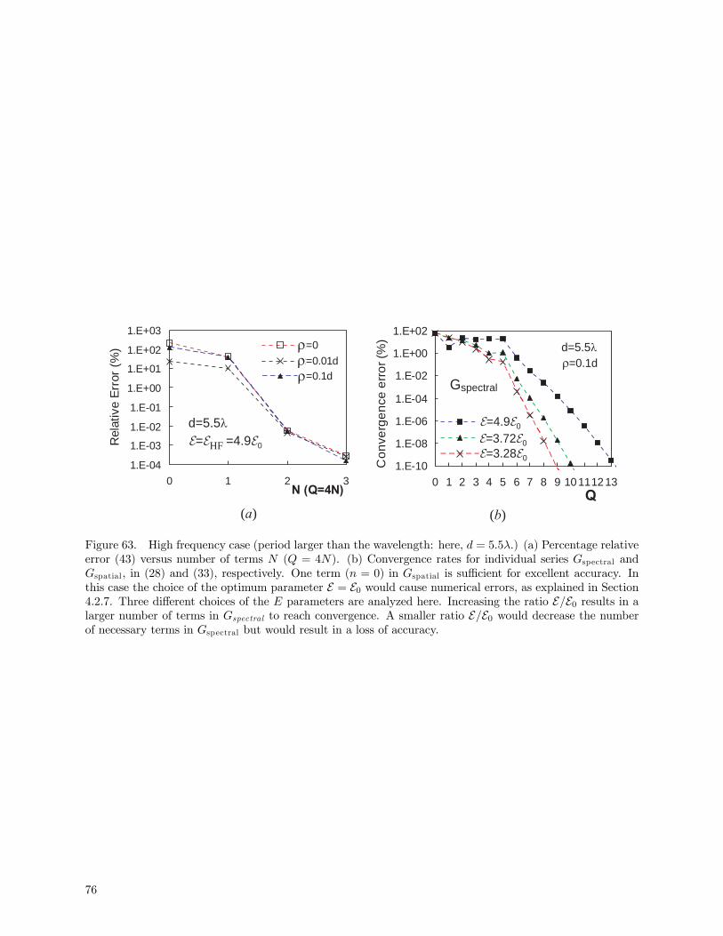
( )b( )a

1.E-04

1.E-03

1.E-02

1.E-01

1.E+00

1.E+01

1.E+02

1.E+03

0 1 2 3N (Q=4N)

Rela

tive

Err

or

(%) x=0

x=0.01d

x=0.1d

1.E-10

1.E-08

1.E-06

1.E-04

1.E-02

1.E+00

1.E+02

0 1 2 3 4 5 6 7 8 9 10111213

Q

Co

nve

rge

nce

err

or

(%)

E =1.57

E =1.19

E =1.05

d=5.5

d=5.5

G

= HF =4.90

=0.1d

spectral

=4.90

=3.720

=3.280

Figure 63. High frequency case (period larger than the wavelength: here, d = 5.5λ.) (a) Percentage relativeerror (43) versus number of terms N (Q = 4N). (b) Convergence rates for individual series Gspectral andGspatial , in (28) and (33), respectively. One term (n = 0) in Gspatial is sufficient for excellent accuracy. Inthis case the choice of the optimum parameter E = E0 would cause numerical errors, as explained in Section4.2.7. Three different choices of the E parameters are analyzed here. Increasing the ratio E/E0 results in alarger number of terms in Gspectral to reach convergence. A smaller ratio E/E0 would decrease the numberof necessary terms in Gspectral but would result in a loss of accuracy.

76

have chosen E = EHF > E0. The spatial series Gspatial needs only the n = 0 term and it is accurate enoughto be off the scale of the plot; hence only the number Q of terms in the spectral series Gspectral is given. Theerror in Figure 63(b) does not decrease significantly before Q = 6 because for this case (d = 5.5λ) spectralterms with |q| ≤ Q = 6 are propagating and must be accounted for to obtain an accurate evaluation of thespectral part of the Ewald representation.

Note that the larger the Ewald parameter, the greater the number of terms needed to achieve the sameaccuracy. The three cases with E = EHF, are relative to EHF = 1.05/λ = 3.28E0, EHF = 1.19/λ = 3.72E0and EHF = 1.57/λ = 4.9E0, where the optimum parameter (not so optimum in this case) is E0 = 0.32/λ.According to (42), these cases correspond to choosing H = 3, 2.64 and 2, respectively. Clearly, as describedin Section 4.2.7, choosing a larger H (i.e., smaller EHF/E0) bounds the growth of the number of terms inGspectral . Unfortunately, H cannot be chosen too large because it would generate values on the order ofeH

2

. It should also be noted that choosing E = EHF, with decreasing H = 3, 2.64, 2, automatically impliesthat the maximum values in the series Gspectral and Gspatial become smaller. For an array with d = 5.5λ,values of H > 3 (i.e., EHF/E0 < 3.28) would already cause a small loss of accuracy, while H < 2 (i.e.,EHF/E0 > 4.9) would require too many terms in the Gspectral sum.4.2.10 Conclusions for 1d Array of Point Sources

The Green’s function (GF) for a linearly-phased, 1d array of point sources has been expressed in termsof two series that exhibit Gaussian convergence as shown in Section 4.2.6. A description of the convergenceproperties, the analysis of the “high frequency breakdown” of the Ewald representation, and its remedy,have been analyzed theoretically and with the help of numerical experiments.

It is important to note that the purely spectral representation of the GF (12), besides being muchslower than the Ewald representation, cannot be evaluated for ρ = 0, which is a very typical situationencountered when analyzing periodic structures of 3D elements with 1D periodicity. In this particular case(ρ = 0) the spatial representation in (9) (sum of spherical waves, which is in general even slower than thespectral representation in (12)) can still be used, rendering the Ewald method even more desirable. Whenit is required to evaluate the Green’s function for complex phasings, the spatial representation cannot beevaluated because it would diverge (as well as the spectral method for ρ = 0), while the Ewald method canbe evaluated also in this case. The Ewald representation is particularly useful for small ρ, while for large ρ(of the order of a period), one can use the well known spectral GF in (12) that is rapidly converging in thisparticular situation. Automatic optimal switching between these two representation for a given accuracyis beyond the scope of this work and will be investigated in the future, as well as an automatic algorithmfor deciding the number of terms to be used in the series, as was done in [66] for the Ewald representationdiscovered in [46].

We are still in the process of adding the Green’s function for the 1d array of point sources to EIGER.Until this is done, we can’t solve the general seam problem. Once we have the code, we may want toapproximate the terms < T,Es (Jpa (x)) > and < T,Es (Jpa0 (x)) > on the right hand side of Equation 8using a high frequency asymptotic approximation. Since the enforcement of the boundary condition alloccurs in the plane of the array we need an expression for the field that is valid there. This is discussednext.

4.3 Approximation of Summation

The asymptotic form of the dipole semi-infinite array is considered on the plane without sources somedistance from the edge. Time dependence ejωt is suppressed and the interelement spacings are dx and dz inthe x and z directions. The exact integral representation is given by

77

E (r) =1

4πdz

∞Xq=−∞

Z ∞−∞

−→G (kx, kyq, kzq)

1− ejdx(kx−γx)e−j(kxx+kyqy+kzqz)

dkxkyq

−→G (kx, ky, kz) =

ζ

k

¡bxkxkz + bykykz + bz ¡k2z − k2¢¢

kρq =qk2 − k2zq

kzq = γz +2πq

dz, q = 0,±1,±2,±3, ...

kyq =qk2 − k2x − k2zq

where γxdx and γzdz are the interelement phase advances in the x and z directions and ζ =pμ0/ε0 is the

free space impedance. The integration contour is deformed above the poles of the integrand and below thebranch point at −kρq, but above the branch point at +kρq.

Letting

kx = kρq cosα

kyq = kρq sinαgives

−→E (−→r ) = 1

4πdx

∞Xq=−∞

ZCα

−→Dq (α) e

−j[kρqρ cos(α−ϕ)+kzqz]dα

x = ρ cosϕ

y = ρ sinϕ

−→Dq (α) =

−→G (kρq cosα, kρq sinα, kzq)

1− ejdx[kρq cosα−γx]

αpq = arccos

µγx + 2πp/dx

kρq

¶= arccos

µkxpkρq

¶

kypq =qk2 − k2xp − k2zq = kρq sinαpq

4.3.1 Asymptotic Expansion of Field

The field is written in terms of a sum of contributions from the residues of Floquet waves (FW ) and a

78

sum of diffraction terms corresponding to the Floquet waves

−→E (−→r ) ∼

∞Xp,q=−∞

−→E FW

pq (−→r )U ¡ϕSBpq − ϕ¢+

∞Xq=−∞

−→E d

q (−→r )

where

−→E FW

pq (−→r ) = 1

2dxdzkypq

−→G (kxp, kypq, kzq) e

−j(kxpx+kzqz+kypqy)

−→G (kx, ky, kz) =

ζ

k

¡bxkxkz + bykykz + bz ¡k2z − k2¢¢

and

−→E d

q (−→r ) =

ZSDP

−→Dq (α) e

−j[kρqρ cos(α−ϕ)+kzqz]dα

U (ϕ) is the unit step function truncating the Floquet waves when the particular pole lies on the steepestdescent path (SDP ) and the corresponding observation angle is at the shadow boundary. The shadowboundaries for the propagating Floquet waves (PFW ) and evanescent Floquet waves (EFW ) are

ϕSBpq = αpq = arccos

µkxpkρq

¶for real kypq (PFW )

ϕSBpq = arccos

µkρqkxp

¶for imaginary kypq (EFW ) and real kρq

ϕSBpq =π

2for imaginary kypq (EFW ) and imaginary kρq

Note that 0 ≤ ϕ ≤ π (the extension is obtained from symmetry arguments).

4.3.2 Diffraction Terms

The evaluation of the diffraction terms is now given. First the function

−→W q (α) =

PXp=−P

[−→w pq− (α) + εp−→w pq+ (α)] , εp = sgn (kxp)

where

−→w pq∓ (α) =−1

2jkypqdx

−→G (kxp,±kypq, kzq)sin ((αpq ∓ α) /2)

is subtracted from the integrand function−→Dq (α) with which it shares the same poles and residues. In

addition the integral of the function−→W q (α) e

−jkρqρ cos(α−ϕ) can be expressed in the closed form on theSDP. Note that the poles extracted include not only those associated with the physical PFW and EFW,but also those associated with improper waves whose presence may influence the behavior of the integrand.In particular wpq+ (α) contains the improper poles. This leads to the asymptotic form

79

−→E d

q (−→r ) ∼ 1

4πdz

s2πj

kρqρe−j(kρqρ+kzqz)

⎡⎣−→T q (ϕ) +PX

p=−P

©−→w pq− (ϕ)F¡δ2pq−

¢+ εp−→w pq+ (ϕ)F

¡δ2pq+

¢ª⎤⎦and

−→T q (α) =

−→Dq (α)−−→W q (α)

This result can be rearranged as

−→E d

q (−→r ) ∼ 1

4πdz

s2πj

kρqρe−j(kρqρ+kzqz)

⎡⎣−→Dq (ϕ) +PX

p=−P

©−→w pq− (ϕ)¡F¡δ2pq−

¢− 1¢+ εp−→w pq+ (ϕ)

¡F¡δ2pq+

¢− 1¢ª⎤⎦

The error function F is the transition function of the UTD

F (x) = 2√xejx

Z ∞√x

e−jt2

dt with − 3π2

< arg (x) ≤ π

2whose arguments are given by

δpq± =p2kρqρ sin

µαpq ± ϕ

2

¶Note that

F¡δ2¢= ±√πejπ/4δejδ2erfc

³±ejπ/4δ

´, Re

³ejπ/4δ

´ ><0

We can also write

F¡δ2¢=√πejπ/4δejδ

2herfc

³ejπ/4δ

´− 2U

³−Re

³ejπ/4δ

´´i4.3.3 Evaluation

We are interested here in evaluating the expression near the plane surface ϕ = 0, π.

δpq± =p2kρqρ sin

µαpq ± ϕ

2

¶

−→E d

q (−→r ) ∼ 1

4πdz

s2πj

kρqρe−j(kρqρ+kzqz)

80

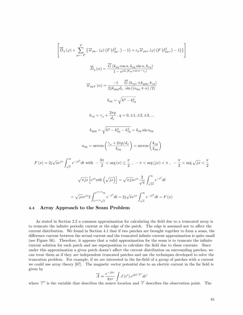
⎡⎣−→Dq (ϕ) +PX

p=−P

©−→w pq− (ϕ)¡F¡δ2pq−

¢− 1¢+ εp−→w pq+ (ϕ)

¡F¡δ2pq+

¢− 1¢ª⎤⎦

−→Dq (α) =

−→G (kρq cosα, kρq sinα, kzq)

1− ejdx[kρq cosα−γx]

−→w pq∓ (α) =−1

2jkypqdx

−→G (kxp,±kypq, kzq)sin ((αpq ∓ α) /2)

kρq =qk2 − k2zq

kzq = γz +2πq

dz, q = 0,±1,±2,±3, ...

kypq =qk2 − k2xp − k2zq = kρq sinαpq

αpq = arccos

µγx + 2πp/dx

kρq

¶= arccos

µkxpkρq

¶

F (x) = 2j√xejx

Z ∞√x

e−jt2

dt with − 3π2

< arg (x) ≤ π

2, − π < arg (jx) < π , − π

2< arg

pjx <

π

2

pπjx

hejxerfc

³pjx´i=pπjxejx

2√π

Z ∞√jx

e−t2

dt

=pjxejx2

Z ejπ/4∞

ejπ/4√x

e−t2

dt = 2j√xejx

Z ∞√x

e−jt2

dt = F (x)

4.4 Array Approach to the Seam Problem

As stated in Section 2.2 a common approximation for calculating the field due to a truncated array isto truncate the infinite periodic current at the edge of the patch. The edge is assumed not to affect thecurrent distribution. We found in Section 4.1 that if two patches are brought together to form a seam, thedifference current between the actual current and the truncated infinite current approximation is quite small(see Figure 56). Therefore, it appears that a valid approximation for the seam is to truncate the infinitecurrent solution for each patch and use superposition to calculate the field due to these currents. Sinceunder this approximation a given patch doesn’t affect the current distribution on surrounding patches, wecan treat them as if they are independent truncated patches and use the techniques developed to solve thetruncation problem. For example, if we are interested in the far-field of a group of patches with a currentwe could use array theory [67]. The magnetic vector potential due to an electric current in the far field isgiven by

−→A ≈ e−jkr

4πr

ZJ (r0) ejkr·

−→r 0dr0

where −→r 0 is the variable that describes the source location and −→r describes the observation point. The

81

Figure 64. FSS illuminated by a plane wave or by a beam source

electric field is related to the vector potential by

Eθ = −jωμAθ

Eφ = −jωμAφ

If the current on every element of a patch are identical except for a complex constant (In) — a phaseprogression, for example — then we can write the field due to the patch as

Eθ =−jωμe−jkr

4πr

∙ZJθ (r

0) ejkr·−→r 0

dr0¸" NX

n−1Ine

jkr·−→r n#

(45)

where −→r n the location of the reference point of each element and N is the number of elements on the patch.The expression for Eφ has a similar form. The second factor of Equation 45 (the integral) is the patternfor a single element of the array and the third factor (the summation) is the array factor. This means thatthe far-field for the patch can be computed using a single integration over one of the elements and a simplesummation over the N elements in the array. The far-field for a number of patches is a sum of the fieldfrom each patch. A further simplification is to use a high frequency expansion like Capolino [21],[23] tocalculate the array factor. This reduces the number of summation terms from N per patch (typically onthe order of a million) to nine per patch. This method is taken up in the following section for truncatedarrays. The diffraction from a seam is a sum of the two truncated edges diffraction contributions bearingin mind that the angle to the observation point are supplementary angles for the two edges.

4.5 High Frequency Approach to the Seam Problem

In this section, we consider a truncated FSS and an FSS having a seam. The scattered fields producedby the edges in such surfaces are described by diffraction phenomena, whose effects are highlighted here.We first consider an FSS illuminated by a plane wave, as shown in Figure 64. It should be noted thatthe discussion that follows can also, in principle, be applied to the case of an incident field produced byproximate antennas or beam sources, assuming that the FSS is in the far field of the radiating antennaor beam source (this restriction may also be removed with a more detailed analysis). For the case of anincident plane wave, we consider an observation point in the near field of the FSS structure.

The diffraction effects from the edges of the truncated periodic structures are the same as those for aPEC plate. The effect of the periodic elements is to weight the amplitude of the various ray species thatarise from the edges and the corners of the FSS, relative to the simple PEC contributions. For example, the

82

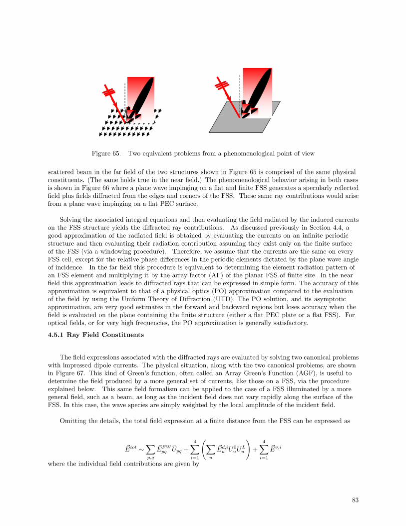
Figure 65. Two equivalent problems from a phenomenological point of view

scattered beam in the far field of the two structures shown in Figure 65 is comprised of the same physicalconstituents. (The same holds true in the near field.) The phenomenological behavior arising in both casesis shown in Figure 66 where a plane wave impinging on a flat and finite FSS generates a specularly reflectedfield plus fields diffracted from the edges and corners of the FSS. These same ray contributions would arisefrom a plane wave impinging on a flat PEC surface.

Solving the associated integral equations and then evaluating the field radiated by the induced currentson the FSS structure yields the diffracted ray contributions. As discussed previously in Section 4.4, agood approximation of the radiated field is obtained by evaluating the currents on an infinite periodicstructure and then evaluating their radiation contribution assuming they exist only on the finite surfaceof the FSS (via a windowing procedure). Therefore, we assume that the currents are the same on everyFSS cell, except for the relative phase differences in the periodic elements dictated by the plane wave angleof incidence. In the far field this procedure is equivalent to determining the element radiation pattern ofan FSS element and multiplying it by the array factor (AF) of the planar FSS of finite size. In the nearfield this approximation leads to diffracted rays that can be expressed in simple form. The accuracy of thisapproximation is equivalent to that of a physical optics (PO) approximation compared to the evaluationof the field by using the Uniform Theory of Diffraction (UTD). The PO solution, and its asymptoticapproximation, are very good estimates in the forward and backward regions but loses accuracy when thefield is evaluated on the plane containing the finite structure (either a flat PEC plate or a flat FSS). Foroptical fields, or for very high frequencies, the PO approximation is generally satisfactory.

4.5.1 Ray Field Constituents

The field expressions associated with the diffracted rays are evaluated by solving two canonical problemswith impressed dipole currents. The physical situation, along with the two canonical problems, are shownin Figure 67. This kind of Green’s function, often called an Array Green’s Function (AGF), is useful todetermine the field produced by a more general set of currents, like those on a FSS, via the procedureexplained below. This same field formalism can be applied to the case of a FSS illuminated by a moregeneral field, such as a beam, as long as the incident field does not vary rapidly along the surface of theFSS. In this case, the wave species are simply weighted by the local amplitude of the incident field.

Omitting the details, the total field expression at a finite distance from the FSS can be expressed as

Etot ∼Xp,q

EFWpq Upq +

4Xi=1

ÃXu

Ed,iu U0uU

Lu

!+

4Xi=1

Ev,i

where the individual field contributions are given by

83

P

Figure 66. A plane wave impinging on a flat FSS generates a reflected field and diffracted fields from theedges and corners of the FSS at the observation point P.

P

Vertex diffracted FW Edge diffracted FW

Floquet Wave (FW)

Vertex diffracted FW Edge diffracted FW

Figure 67. The three wave species, the reflected field, the edge diffracted field, and corner (or vertex)diffracted field arriving at the observation point P. Also shown are the two canonical problems that can beused to determine the mathematical form of these ray contributions.

84

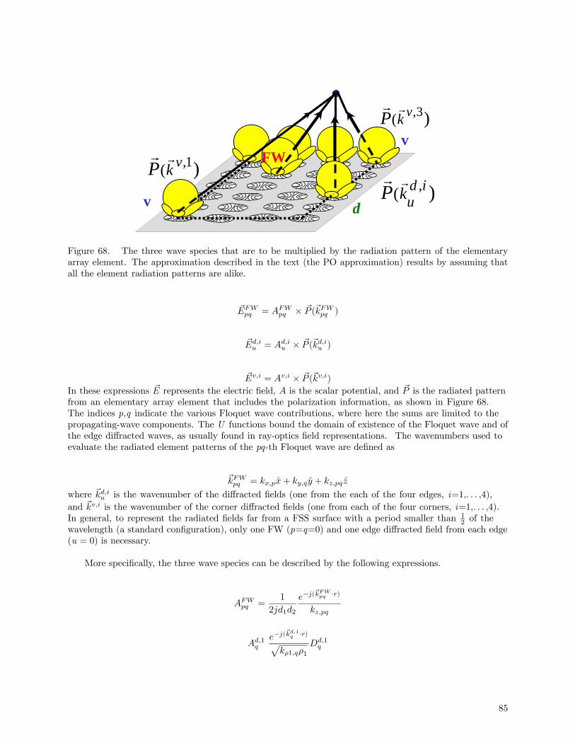
v

FW

d

v ,1( )vkP

rr

,( )d iukPrr

,3( )vkPrr

Figure 68. The three wave species that are to be multiplied by the radiation pattern of the elementaryarray element. The approximation described in the text (the PO approximation) results by assuming thatall the element radiation patterns are alike.

EFWpq = AFW

pq × P (kFWpq )

Ed,iu = Ad,i

u × P (kd,iu )

Ev,i = Av,i × P (kv,i)

In these expressions E represents the electric field, A is the scalar potential, and P is the radiated patternfrom an elementary array element that includes the polarization information, as shown in Figure 68.The indices p,q indicate the various Floquet wave contributions, where here the sums are limited to thepropagating-wave components. The U functions bound the domain of existence of the Floquet wave and ofthe edge diffracted waves, as usually found in ray-optics field representations. The wavenumbers used toevaluate the radiated element patterns of the pq-th Floquet wave are defined as

kFWpq = kx,px+ ky,qy + kz,pq z

where kd,iu is the wavenumber of the diffracted fields (one from the each of the four edges, i=1,. . . ,4),and kv,i is the wavenumber of the corner diffracted fields (one from each of the four corners, i=1,. . . ,4).In general, to represent the radiated fields far from a FSS surface with a period smaller than 1

2 of thewavelength (a standard configuration), only one FW (p=q=0) and one edge diffracted field from each edge(u = 0) is necessary.

More specifically, the three wave species can be described by the following expressions.

AFWpq =

1

2jd1d2

e−j(kFWpq ·r)

kz,pq

Ad,1q

e−j(kd,1q ·r)p

kρ1,qρ1Dd,1q

85

Av,1 e−jkr

rDv,1

Here we have highlighted the plane-wave behavior for the Floquet wave AFWpq , d1 and d2 are the two

periods along bx and by, respectively. We have also highlighted the cylindrical and the spherical spreadingfactors for the edge and corner diffracted fields, whereas Dd,1

q and Dv,1 represent the edge and cornerdiffraction coefficients that involve the transition function of the Uniform Theory of Diffraction, and a morecomplicated transition function for the corner diffraction coefficient. Further details can be found in [21]—[23] and are not given here due to space constraints.

We stress again that the above field description assumes that the current on all the FSS elements,illuminated by a plane wave, is the same excluding a phase factor dictated by the specific plane-waveexcitation. In other words, we assume that all the array elements produce the same radiated fields.Elements near the edges (or near a seam between two FSS) would, in reality, have different currents, butthe overall radiated field in the forward or backward direction is not significantly affected by these currentmodifications. This is examined in the numerical examples presented below.

4.5.2 Algorithm for the Field Evaluation

We provide here a simple way to approximate the radiated field produced by a truncated FSSfor two illuminating conditions: a plane wave and a beam. (The case of a seam formed between twofrequency-selective surfaces is analogous.) The approximation is as described above, in that all the FSSelements have the same current besides the phase differences dictated by the incident field.

Plane Wave Excitation• The currents on an elementary cell (of the array) are found by a solver for periodic structures.

• The radiation pattern of an elementary array cell (a cell of the FSS) can be easily evaluated by usinga Fourier transform of the array element current every time it is needed, or it is evaluated beforehand,sampled and then interpolated.

• For each of the 9 ray contributions (associated with 4 corners, 4 edges, and a reflected ray from the flatsurface) that reach the observer at finite distance away, we evaluate the radiation pattern (one for eachray) as a function of the observation point. The radiation patterns are then multiplied by the ray fieldcontributions.

Near Field Excitation (e.g., Horn Antenna)• The direction of incidence of the various 9 rays (for rectangular FSS) are evaluated by a standard andsimple ray tracing.

• For each of these 9 incidence angles, the currents on an elementary periodic FSS cell are evaluated byusing a solver for periodic structures. Then, the 9 set of currents are stored.

• The 9 radiation patterns can be easily evaluated by using a Fourier transform of the array elementcurrent every time they are needed, or they are evaluated beforehand, sampled and then interpolated.

• For each of the 9 rays contributions that reach the observer (at finite distance) we evaluate the radiationpattern (one for each ray) that is a function of the direction of observation. The radiation patterns arethen multiplied by the ray field contributions.

86

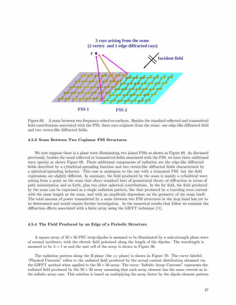
P

FSS 1 FSS 2

Incident field

3 rays arising from the seam(2 vertex- and 1 edge-diffracted rays)

Figure 69. A seam between two frequency-selective-surfaces. Besides the standard reflected and transmittedfield contributions associated with the FSS, three rays originate from the seam: one edge-like diffracted fieldand two vertex-like diffracted fields.

4.5.3 Seam Between Two Coplanar FSS Structures

We now suppose there is a plane wave illuminating two joined FSSs as shown in Figure 69. As discussedpreviously, besides the usual reflected or transmitted fields associated with the FSS, we have three additionalwave species as shown Figure 69. These additional components of radiation are the edge-like diffractedfields described by a cylindrical-spreading function and two vertex-like diffracted fields characterized bya spherical-spreading behavior. This case is analogous to the one with a truncated FSS, but the fieldexpressions are slightly different. In summary, the field produced by the seam is mainly a cylindrical wavearising from a point on the seam that obeys standard laws of geometrical theory of diffraction in terms ofpath minimization and so forth, plus two other spherical contributions. In the far field, the field producedby the seam can be expressed as a single radiation pattern, like that produced by a traveling wave currentwith the same length as the seam, and with an amplitude dependant on the geometry of the seam itself.The total amount of power transmitted by a seam between two FSS structures in the stop band has yet tobe determined and would require further investigation. In the numerical results that follow we examine thediffraction effects associated with a finite array using the GIFFT technique [11].

4.5.4 The Field Produced by an Edge of a Periodic Structure

A square array of 50× 50 PEC strip-dipoles is assumed to be illuminated by a unit-strength plane waveof normal incidence, with the electric field polarized along the length of the dipoles. The wavelength isassumed to be λ = 1 m and the unit cell of the array is shown in Figure 36.

The radiation pattern along the E-plane (the xz plane) is shown in Figure 70. The curve labeled“Physical Currents” refers to the radiated field produced by the actual current distribution obtained viathe GIFFT method when applied to the 50× 50 array. The curve “Infinite Array Currents” represents theradiated field produced by the 50× 50 array assuming that each array element has the same current as inthe infinite array case. This solution is based on multiplying the array factor by the dipole element pattern

87

-90

-45

0

45

90

135

180

225

-60

-20

-20

20

20

40

40

60

60

50X50: Physical Currents50X50: Infinite Array Currents50X50: Fringing Current Only

0

Figure 70. The far-field E-plane radiation pattern produced by the 50× 50 dipole array.

in the infinite array environment. The curve labeled “Fringing Current Only” refers to the field producedby the 50 × 50 array when the strip-dipole elements contain currents equal to the difference between theactual current and the infinite array current solution. The fringing current is dominant near the array edgesand tends to zero toward the center where the infinite array current is a good approximation, assumingthat there are no surface waves excited in the periodic structure (as should be the situation in the presentcase). Figure 70 shows that the fringing current produces a negligible field effect away from the planecontaining the array. Due to the fact that the fringe current is mainly comprised of a traveling wave witha wavenumber equal to that of free space (grazing propagation), the fringe effect is visible in the angularrange between 70 and 90 degrees.. This example also demonstrates that away from grazing the “InfiniteArray Currents” solution is an effective tool to predict the field since it avoids the need to grid the entirearray.

The near-field behavior can be described in terms of a modified GTD (Geometrical Theory ofDiffraction) ray theory, based on the Floquet-wave modulation of the diffraction coefficients [70]. To showthis behavior, we plot the electric near field moving away from an edge along the observation scan shown inFigure 71. The observation scan is chosen in such a way to allow us to neglect the field arising from thefour corners and the other three edges.

Figure 72 shows the electric field along the scan in Figure 71 produced by the three set of currentsassociated with the patterns in Figure 70. It is evident that they all decrease with the same trend whenmoving away from the edge. As already noted in Figure 70, the field produced by the “Fringing CurrentsOnly” is significant at grazing. Along other angular directions this field contribution is in general smallerthan the other two contributions in Figure 72. The small ripple may be associated with the diffractioneffects due to the other edges and corners.

88

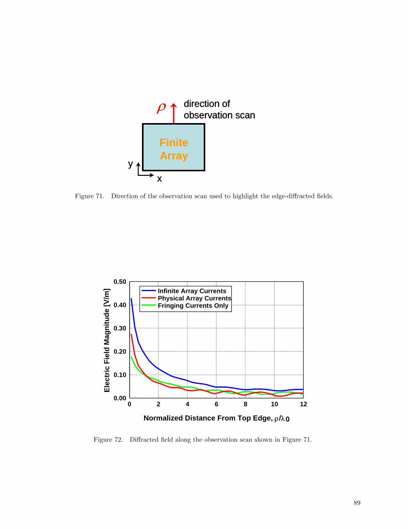
FiniteArray

xy

ρ direction of observation scan

FiniteArray

xy

ρ direction of observation scan

Figure 71. Direction of the observation scan used to highlight the edge-diffracted fields.

0 2 4 6 8 10 12

Normalized Distance From Top Edge, ρ/λ0

0.00

0.10

0.20

0.30

0.40

0.50

Elec

tric

Fie

ld M

agni

tude

[V/m

] Infinite Array CurrentsPhysical Array CurrentsFringing Currents Only

Figure 72. Diffracted field along the observation scan shown in Figure 71.

89

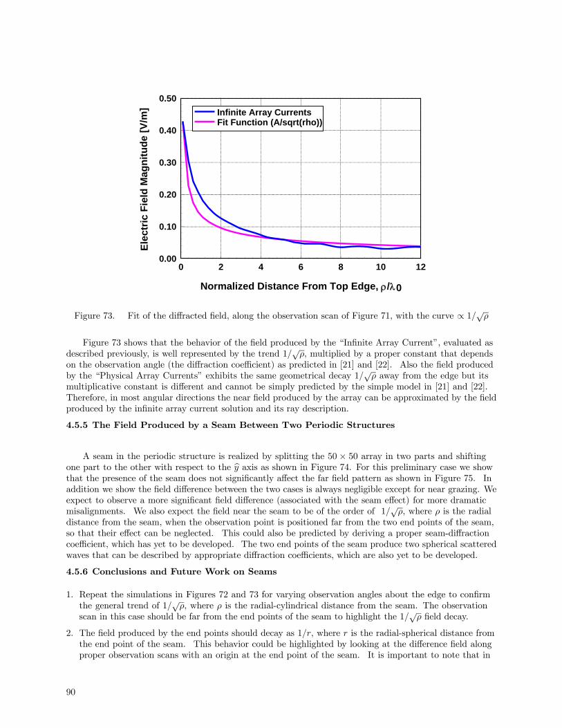
0 2 4 6 8 10 12

Normalized Distance From Top Edge, ρ/λ0

0.00

0.10

0.20

0.30

0.40

0.50

Elec

tric

Fie

ld M

agni

tude

[V/m

] Infinite Array CurrentsFit Function (A/sqrt(rho))

Figure 73. Fit of the diffracted field, along the observation scan of Figure 71, with the curve ∝ 1/√ρ

Figure 73 shows that the behavior of the field produced by the “Infinite Array Current”, evaluated asdescribed previously, is well represented by the trend 1/

√ρ, multiplied by a proper constant that depends

on the observation angle (the diffraction coefficient) as predicted in [21] and [22]. Also the field producedby the “Physical Array Currents” exhibits the same geometrical decay 1/

√ρ away from the edge but its

multiplicative constant is different and cannot be simply predicted by the simple model in [21] and [22].Therefore, in most angular directions the near field produced by the array can be approximated by the fieldproduced by the infinite array current solution and its ray description.

4.5.5 The Field Produced by a Seam Between Two Periodic Structures

A seam in the periodic structure is realized by splitting the 50 × 50 array in two parts and shiftingone part to the other with respect to the by axis as shown in Figure 74. For this preliminary case we showthat the presence of the seam does not significantly affect the far field pattern as shown in Figure 75. Inaddition we show the field difference between the two cases is always negligible except for near grazing. Weexpect to observe a more significant field difference (associated with the seam effect) for more dramaticmisalignments. We also expect the field near the seam to be of the order of 1/

√ρ, where ρ is the radial

distance from the seam, when the observation point is positioned far from the two end points of the seam,so that their effect can be neglected. This could also be predicted by deriving a proper seam-diffractioncoefficient, which has yet to be developed. The two end points of the seam produce two spherical scatteredwaves that can be described by appropriate diffraction coefficients, which are also yet to be developed.

4.5.6 Conclusions and Future Work on Seams

1. Repeat the simulations in Figures 72 and 73 for varying observation angles about the edge to confirmthe general trend of 1/

√ρ, where ρ is the radial-cylindrical distance from the seam. The observation

scan in this case should be far from the end points of the seam to highlight the 1/√ρ field decay.

2. The field produced by the end points should decay as 1/r, where r is the radial-spherical distance fromthe end point of the seam. This behavior could be highlighted by looking at the difference field alongproper observation scans with an origin at the end point of the seam. It is important to note that in

90

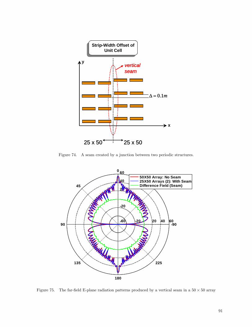
x

yvertical seam

Strip-Width Offset of Unit Cell

Strip-Width Offset of Unit Cell

25 x 5025 x 50

0.1mΔ =

x

yvertical seam

x

yvertical seam

Strip-Width Offset of Unit Cell

Strip-Width Offset of Unit Cell

25 x 5025 x 50

0.1mΔ =

Figure 74. A seam created by a junction between two periodic structures.

-90

-45

0

45

90

135

180

225

-60

-20

-20

20

20

40

40

60

60

50X50 Array: No Seam25X50 Arrays (2): With SeamDifference Field (Seam)

Figure 75. The far-field E-plane radiation patterns produced by a vertical seam in a 50× 50 array

91

practical designs the end points are present and the estimation of effects in this finite array environment(where all the effects are combined) could provide valuable information to the FSS designer.

3. Determine the diffraction coefficient associated with the seam by fitting the numerical results withtheoretical predictions.

4. An efficient tool to isolate the seam effect is the linear-array Green’s function (see Section 4.2) thatallows the modeling of periodic structures that are infinitely long along the by axis, thus removing theend point effects. Since the numerical burden of the problem is that of only one row (along bx), verywide structures (along bx) could be easily modeled. This work is currently being carried out via theimplementation of the linear array Green’s function into EIGER.

5. The simulation of a finite array with one or more defects is easily handled by GIFFT. Using GIFFT,we could estimate the total amount of power that passes through a seam of a particular FSS.

6. Further development is needed in GIFFT to model an FSS where current can flow across unit cellboundaries. At present, current unknowns are confined to reside within a unit cell.

5 Conclusions

In this LDRD we have looked at various techniques to analyze structures that depart from periodicity.We examined single point defects, truncations and seams. A general statement is that compared to thespecular reflection or transmission, the scattering from breaks in periodicity plays a minor role. It is onlyif we are at an observation point where the specular is suppressed that the breaks in periodicity begin tocontribute. Scattering from truncation seems to be greater than scattering from seams, which seems to begreater than scattering from a single defect.

We modified GIFFT to handle two types of unit cells on the same periodic lattice. Using this we couldanalyze single defects (where one unit cell is different from all the rest) or a seam (where a group of half theunit cells differ from the other half). We used GIFFT to confirm the behavior of fields near a truncatededge as being the same as that calculated using diffraction. We are in the process of incorporating GIFFTinto EIGER.

An isolated defect seems to be ignorable. If we want to modify the bandgap, it appears that we haveto add a periodic defect which can be analyzed using the well-known periodic techniques with a unit cellthat encompasses the new periodicity.

To complete the work started here we need to finish incorporating GIFFT and the 1D array of pointsources in EIGER. We should then implement techniques in EIGER to analyze the 2d seam and compareto the other techniques developed here (GIFFT and the asymptotic high frequency solution). Both GIFFTand the one-dimensional seam problem indicate that the majority of the seam and truncation effect ismodeled by truncating the infinite periodic solution. If that conclusion is unaltered after further testing,we can write software to analyze groups of these patches. Since the patches are all independent of eachother, we can use superposition and the various approximations described in Sections 4.4 and 4.5.

6 References

[1] E. Yablonovitch, “Photonic crystals: semiconductors of light,” Scientific American, pp. 47-55,December 2001.

[2] E. Yablonovitch, “Inhibited spontaneous emission in solid-state physics and electronics,” Physical

92

Review Letters, vol. 58. no. 20, pp. 2059-2062, 18 May 1987.

[3] T. Cwik and R. Mittra, “Scattering from a periodic array of free-standing, arbitrarily shaped, perfectlyconducting or resistive patches,” IEEE Trans. Antennas and Propagat., vol. 35, no. 11, pp. 1226-1234,Nov. 1987.

[4] Y. Rahmat-Samii and A. N. Tulintseff, “Diffraction analysis of frequency selective reflector antennas,”IEEE Trans. Antennas and Propagat., vol. 41, no. 4, pp. 476-487, April 1993.

[5] J. S. McCalmont, M. M. Sigalas, G. Tuttle, K. M. Ho and C. M. Soukolis, “A layer-by-layer metallicphotonic band-gap structure,” Appl. Phys. Lett., vol. 68, no. 19, pp. 2759 - 2761, 6 May 1996.

[6] V. V. S. Prakash and R. Mittra, “Technique for analyzing cascaded frequency selective surface screenswith dissimilar lattice geometries,” IEE Proc. Microw. Antennas Propagat., vol. 150, no. 1, pp. 23 -27, February 2003.

[7] E. Yablonovitch, T. J. Gmitter, R. D. Meade, A. M. Rappe, K. D. Brommer and J. D. Jonnopoulos,“Donor and acceptor modes in photonic band structure,”Physical Review Letters, vol. 67, no. 24, pp.3380-3389, December 1991.

[8] J. B. Pendry, “Photonic band structures,” Journal of Modern Optics, vol. 41, no. 2, pp. 209-229, 1994.

[9] M. L. Povinelli, S. G. Johnson, S. Fan and J. D. Joannopoulos, “Emulation of two-dimensionalphotonic crystal defect modes in a photonic crystal with a three-dimensional photonic band gap,”Physical Review B, vol. 64, no. 7, article no. 075313, 2001

[10] R. Mittra, C. H. Chan and T. Cwik, “Techniques for analyzing frequency selective surfaces — a review,”IEEE Proc., vol. 76, pp. 1693-1615, Dec. 1988.

[11] B.J. Fasenfest, F. Capolino, D.R. Wilton, and D.R. Jackson, N. Champagne, “A fast MOM solutionfor large arrays: Green’s function interpolation with FFT,” IEEE Antennas and Wireless PropagationLetters, vol. 3, pp. 161-164, 2004.

[12] B. Fasenfest, Fast Computation for Large Arrays, Masters Dissertation, Univ. Houston, Houston, TX2004

[13] E. Bleszynski, M. Bleszynski, and T. Jaroszewicz, “AIM: Adaptive integral method for solving largescale electromagnetic scattering and radiation problems,” Radio Science, vol. 31, pp. 1225-1251, 1996.

[14] T. Cwik and R. Mittra, “The effects of the truncation and curvature of periodic surfaces: a stripgrating,” IEEE Trans. Antennas and Propagat., vol. 36, no. 5, pp. 612-622, May 1988.

[15] W. L. Ko, and R. Mittra, “Scattering by a truncated periodic array,” IEEE Trans. Antennas andPropagat., vol. 36, no. 4, pp. 496-502, April 1988.

[16] K. O. Merewether and R. Mittra, “Spectral-domain analysis of a finite frequency-selective surface withcross-shaped conducting patches,” 1988 International Symposium Digest: Antennas and Propagation,vol.2, pp. 742-745, 1988.

[17] B. Philips, E. A. Parker, R. J. Langley, “Ray tracing analysis of the transmission performance ofcurved FSS,” IEE Proceedings on Microwave and Antennas Propagat., vol. 142, no. 3, pp. 193-199,June 1995.

[18] H. Ling, R. C. Chou, S. W. Lee, “Shooting and bouncing rays: Calculating the RCS of an arbitrarilyshaped cavity,” IEEE Trans. Antennas and Propagat., vol. 37, no. 2, pp. 194-205, Feb. 1989.

[19] A. Ishimaru, R. J. Coe, G. E. Miller and W. P. Geren, “Finite periodic structure approach to largescanning array problems,” IEEE Trans. Antennas and Propagat., vol. 33, no. 11, pp. 1213-1219, Nov.1985.

[20] L. Carin and L. B. Felsen, “Time harmonic and transient scattering by finite periodic flat strip arrays:Hybrid (ray)-(Floquet mode)-(MOM) algorithm,” IEEE Trans. Antennas and Propagat., vol. 41, no.4, pp. 412-421, Apr. 1993.

[21] F. Capoliino, M. Albani, S. Maci, L. B. Felsen, “Frequency domain Green’s function for a planarperiodic semi-infinite phased array: Part I: Truncated Floquet wave formulation,” IEEE Transactions

93

on Antennas and Propagation, vol. 48, no. 1, pp. 67-74, Jan. 2000.

[22] F. Capolino, M. Albani, S. Maci, and L.B. Felsen,“Frequency domain Green’s function for a planarperiodic semi-infinite phased array. Part II: Phenomenology of the diffracted waves,” IEEE Trans.Antennas and Propagation, vol. 48, no.1, pp. 75-85, Jan. 2000.

[23] F. Capolino, S. Maci and L.B. Felsen, “Green’s function for a planar phased sectoral array of dipoles,”Radio Science, Special Issue on the 1998 URSI Intern. Symp. on EM Theory, vol. 35, no. 2, pp.579-593, March-April, 2000.

[24] V. V. S. Prakash and R. Mittra, “Convergence studies of plane-wave spectral expansion technique foranalyzing truncated frequency-selective surfaces,” Microwave and Optical Technology Letters, vol. 34,no. 6, pp. 417-421, Sept. 20, 2002.

[25] A. Neto, S. Maci, G. Vecchi, and M. Sabbadini, “A truncated Floquet wave diffraction method forthe full wave analysis of large phased arrays — Part I: Basic principles and 2-d cases,” IEEE Trans.Antennas and Propagat., vol. 48, no. 3, pp. 594-600, March 2000.

[26] A. Neto, S. Maci, G. Vecchi, and M. Sabbadini, “A truncated Floquet wave diffraction method forthe full wave analysis of large phased arrays — Part II: Generalization to 3-d cases,” IEEE Trans.Antennas and Propagat., vol. 48, no. 3, pp. 601-611, March 2000.

[27] A. Cucini, M. Albani, S. Maci, “Truncated Floquet wave full-wave³T (FW )

2´analysis of large

periodic arrays of rectangular waveguides,” IEEE Trans. Antennas and Propagat., vol. 51, no. 6, pp.1373-1385, June 2003.

[28] O. A. Civi, P. H. Pathak, H. T. Chou, P. Nepa, “A hybrid uniform geometrical theory of diffraction —moment method for efficient analysis of electromagnetic radiation/scattering from large finite planararrays,” Radio Science, vol. 35, no. 2, pp. 607-620, March-April 2000.

[29] B. A. Munk, D. S. Janning, J. B. Pryor and R. J. Marhefka, “Scattering from surface waves on finiteFSS,” IEEE Trans. Antennas and Propagat., vol. 49 no. 12, pp. 1782-1792, Dec. 2001.

[30] M. P. Hurst, “Improved numerical diffraction coefficients with application to frequency selectivesurfaces,” IEEE Trans. Antennas and Propagat., vol. 40, no. 6, pp. 606-212, June 1992.

[31] G. Pelosi, G. Manara, G. Toso, “Heuristic diffraction coefficient for plane-wave scattering from edgesin periodic planar surfaces,” J. Opt. Soc. Am. A, vol. 13, no. 8, pp. 1689-1697, Aug. 1996.

[32] S. Q. Li, Y. Yu, C. H. Chan, K. F. Chan, and L. Tsang, “A sparse-matrix/canonical grid method foranalyzing densely packed interconnects,” IEEE Trans. Microwave Theory Tech., vol. 49, no. 7, pp.1221-1228, July 2001.

[33] L. Tsang, C. H. Chan, P. Kyung, H. Sangani, “Monte-Carlo simulations of large-scale problems ofrandom rough surface scattering and applications to grazing incidence with the BMIA/canonical gridmethod,” IEEE Trans. Antennas and Propagat., vol. 43, no. 8, pp. 851-859, Aug. 1995.

[34] S. M. Seo, J.F. Lee, “A fast IE-FFT algorithm for solving PEC scattering problems,” IEEE Trans. onMagnetics, vol. 41, no.5, pp. 1476-1479, May 2005.

[35] Mori, F. De Vita, A. Freni, “A modification of the canonical grid series expansion in order to increasethe efficiency of the SMCG method,” IEEE Geoscience and Remote Sensing Letters, vol. 2, no. 1, pp.87-89, Jan. 2005.

[36] R. Coifman, V. Rokhlin, and S. Wandzura, “The fast multipole method for the wave equation: apedestrian prescription,” IEEE Antennas Propagat. Mag., vol. 35, no 3, pp. 7-12, June 1993.

[37] W. C. Chew, J. M. Jin, C. C. Lu, E. Michielssen, J. M. Song, “Fast solution methods inelectromagnetics,” IEEE Trans. Antennas and Propagat., vol. 45, no. 3, pp. 533 — 543, March 1997.

[38] J. Song, C.-C. Lu, W. C. Chew, “Multilevel fast multipole algorithm for electromagnetic scattering bylarge complex objects,” IEEE Trans. Antennas and Propagat., vol. 45, no. 10, pp. 1488 — 1493, Oct.1997.

[39] R. W. Kindt and J. L. Volakis, “Array decomposition-fast multipole method for finite array analysis,”

94

Radio Science, vol. 39, RS2018, 2004

[40] S. M. Rao, D.R. Wilton, and A.W. Glisson, “Electromagnetic scattering by surfaces of arbitraryshape,” IEEE Trans. on Antennas and Propagat., vol. 30, no. 3, pp. 409-418, May 1982.

[41] A. Erentok, P. L. Luljak, and R. W. Ziolkowski, “Characterization of a volumetric meta-materialrealization of an artificial magnetic conductor for antenna applications,” IEEE Trans. Antennas andPropagat., vol. 53, no. 1, pp. 160-172, January 2005.

[42] W. A. Johnson, R. E. Jorgenson, L. K. Warne, J. D. Kotulski, J. B. Grant, R. M. Sharpe, N.J. Champagne, D. R. Wilton, and D. R. Jackson, “Our experiences with object-oriented design,FORTRAN 90, and massively parallel computations,” 1998 Digest USNC/URSI National RadioScience Meeting, June 21-26, 1998, Atlanta, Georgia, Antennas: Gateways to the Global Network, p.308, 1998.

[43] L I. Basilio, W. A. Johnson, D. R. Jackson, and D. R. Wilton, “Numerical modeling of finite-sizeplasmon structures with enhanced optical transmission using EIGER,” Proceedings of Joint 9thInternational Conference on Electromagnetics in Advanced Applications ICEAA 2005 and 11thEuropean Electromagnetic Structures Conference EESC 2005, Torino, Italy, pp. 877- 880, Sept 12-16,2005.

[44] C. R. Simovski, P. de Maagt, I. V. Melchakova, “High impedance surfaces having stable resonancewith respect to polarization and incidence angle,” IEEE Transactions on Antennas and Propagat., vol.53, no. 3, pp. 908-914, March 2005.

[45] P. P. Ewald, “Die berechnung optischer und elektrostatischen gitterpotentiale,” Ann. der Physik, vol.64, pp. 253—287, 1921. Translated by A. Cornell, Atomics International Library, 1964.

[46] K. E. Jordan, G. R. Richter, and P. Sheng, “An efficient numerical evaluation of the Green’s functionfor the Helmholtz operator on periodic structures,” J. Comp. Physics, vol. 63, pp. 222—235, 1986.

[47] D. R. Jackson D. R. Wilton and N. J. Champagne, “Efficient computation of periodic and nonperiodicGreen’s function in layered media using the MPIE,” in URSI Int. Symp. on Electrom. Theory,Thessaloniki, Greece, May. 25-28. 1998.

[48] M. J. Park and S. Nam, “Efficient calculation of the Green’s function for multilayered planar periodicstructures,” IEEE Trans. Antennas Propagat., vol. 46, no. 10, pp. 1582—1583, October 1998.

[49] Y. X. Yu and C. H. Chan, “On the extension of Ewald’s method to periodic structures in layeredmedia,” Microwaves and Optical Techn. Lett., vol. 19, no. 2, pp. 125—131, 1998.

[50] D. Wang, E. K. N. Yung, R. S. Chen, D. Z. Ding, W. C. Tang, “On evaluation of the Green’s functionfor periodic structures in layered media,” IEEE Antennas and Wireless Propagat. Lett., vol. 3, no. 1,pp. 133—136, Sept. 2004.

[51] A. W. Mathis and A. F. Peterson, “A comparison of acceleration procedures for the two-dimensionalperiodic Green’s function,” IEEE Trans. Antennas Propagat., vol. 44, no. 4, pp. 567—571, April 1996.

[52] C. M. Linton, “The Green’s function for the two-dimensional Helmholtz equation in periodic domains,”Journal of Engineering Mathematics, vol. 33, pp. 377—402, 1998.

[53] F. Capolino, D. R. Wilton, and W. A. Johnson, “Efficient computation of the 2d Green’s function for1d periodic structures using the Ewald method,” IEEE Trans. Antennas Propagat., vol. 53, no.5, pp.2977—2984, Sept. 2005.

[54] A. Moroz, “Exponentially convergent lattice sums,” Opt. Lett., vol. 26, pp.1119—1121, 2001.

[55] C. M. Linton, “Schlömilch series that arise in diffraction theory and their efficient computation,”Journal of Physics A, vol. 39, pp. 3325—3339, March 2006.

[56] V. G. Papanicolaou, “Ewald’s method revisited: rapidly convergent series representations of certainGreen’s functions,” Journal of Comp. Analysis and Appl., vol. 1, no. 1, pp. 105-114, 1999.

[57] E. Cohen, “Critical distance for grating lobe series,” IEEE Trans. Antennas Propagat., vol. 39, no. 5,pp. 677—679, May 1991.

95

[58] M. J. Park, J. Park, and S. Nam, “Efficient calculation of the Green’s function for the rectangularcavity,” IEEE Microwave and Guided Wave Lett., vol. 8, no. 3, pp. 124—126, March 1998.

[59] F. Marliani and A. Ciccolella, “Computationally efficient expressions of the dyadic Green’s functionfor rectangular enclosures,” Progress In Electromagnetics Research, PIER, vol. 31, pp. 195-223, 2001.

[60] T. F. Eibert, J. L. Volakis, D. R. Wilton, D. R. Jackson, “Hybrid FE/BI modeling of 3-D doublyperiodic structures utilizing triangular prismatic elements and an MPIE formulation accelerated bythe Ewald transformation,” IEEE Trans. Antennas Propagat., vol. 47, no. 5, pp. 843—850, May 1999.

[61] M. Bressan, L. Perregrini, and E. Regini, “BI-RME modeling of 3D waveguide components enhancedby the Ewald technique,” IEEE MTT-S Int. Microwave Symp. Dig., vol. 2, pp. 1097-1100, 2000.

[62] A. Kustepely and A. Q. Martin, “On the splitting parameter in the Ewald method,” IEEE Trans.Microwave and Guid. Wave Lett., vol. 10, no. 5, pp. 168—170, May 2000.

[63] A. Papoulis, Systems and Transforms with Application in Optics, R.E. Krieger Pub. Co, Malabar, FL,1981.

[64] M. Abramowitz and I.A. Stegun, Handbook of Mathematical Functions, Dover, New York, 1970.

[65] J. A. C. Weideman, “Computation of the complex error function,” SIAM J. Numer. Anal., vol. 31,no. 5, pp. 1497—1518, 1994.

[66] S. Oroskar, D. J. Jackson, D. R. Wilton, “Efficient computation of the 2d periodic Green’s functionusing the ewald Method,” J. Comp. Physics, in print, 2006.

[67] R. F. Harrington,Time Harmonic Electromagnetic Fields, McGraw-Hill: New York, pp.132-134, 1961.

[68] Y. T. Lo and S. W. Lee, Antenna Handbook, Van Nostrand Reinhold Company, New York, chapter11, 1988.

[69] S. Maci, F. Capolino and L.B. Felsen, “Three-dimensional Green’s function for truncated planarperiodic dipole arrays,” Wave Motion — Special Issue on Electrodynamics in Complex Environments,vol. 34, no. 3, pp. 263-279, Sept. 2001.

[70] F. Mariottini, F. Capolino, S. Maci and L.B. Felsen, “Floquet wave diffraction theory for taperedplanar array Green’s function,” IEEE Trans. Antennas and Propagat., vol. 53, no. 2, pp. 608-620, Feb.2005.

96

Distribution:1 Prof. Don R. WiltonUniversity of HoustonDepartment of Electrical and Computer EngineeringHouston, TX 77204-4005

1 Prof. Filippo CapolinoUniversity of HoustonDepartment of Electrical and Computer EngineeringHouston, TX 77204-4005

1 MS1082 J. J. Hudgens, 017251 MS1082 D. W. Peters, 017271 MS1152 R. E. Jorgenson, 016521 MS1152 L. K. Warne, 016521 MS1152 L. I. Basilio, 016521 MS1152 W. A. Johnson, 016521 MS1152 M. L. Kiefer, 016522 MS9018 Central Technical Files, 089442 MS0899 Technical Library, 045361 MS0123 D. L. Chavez, 01011

97