Master’s Thesis

Multiple electromagnetic scattering byspheres using the T-matrix formulation

Marina Wallin

December, 2015

Master’s Thesis, Civilingenjorsprogrammet i teknisk fysik, Umea University.Marina Wallin, mava0049@student.umu.se.

Multiple electromagnetic scattering by spheres using the T-matrix formulationis a project during the course Master’s Thesis in Engineering Physics, 30.0 ECTSat the Department of Physics, Umea University.

Supervisor: Torleif Martin, Saab AB.Examiner: Gert Brodin, Department of Physics, Umea University.

Multiple electromagnetic scattering byspheres using the T-matrix formulation

Abstract

Low observable technology is used in order to prevent detection, or to delay detection. Radar crosssection is an important parameter in aircraft survivability since it measures how detectable an ob-ject is with radar. To find the radar cross section Maxwell’s equations are solved numerically inthe time-domain using a finite difference scheme. This numerical method called Finite DifferenceTime Domain is very suitable for structures including complex materials. However, this numer-ical method needs to be verified for large scale simulations, due to numerical dispersion errors.Therefore it is desirable to verify the accuracy of the numerical simulations. In this project, theanalytical solution to the multiple scattering by two spheres is implemented using the T-matrixformulation. The analytical solution to the scattering problem is first validated with the analyticalMie-series solution then compared to the Finite Difference Time Domain implementation. Theresults imply that the difference between the numerical and analytical solution is larger for higherfrequencies and larger computational volumes.

Keywords: T-matrix, Multiple scattering, RCS, FDTD, Electromagnetic scattering, Mie scat-tering

iii

Elektromagnetisk multipelspridning fransfarer med T-matrismetoden

Sammanfattning

Smygteknik anvands for att forhindra detektering, eller for att fordroja detektion av ett flygplan.Radarmalarea ar en viktig parameter for skyddsprestanda hos flygplan eftersom den mater hurdetekterbar ett foremal ar med radar. For att hitta radarmalarean loses Maxwells ekvationer nu-meriskt i tidsdomanen med hjalp av ett finit differensschema. Den numeriska metoden som kallasFinita differensmetoden i tidsdoman, ar mycket lamplig for strukturer med komplexa material.Den numeriska metoden behover valideras for storskaliga simuleringar eftersom det forekommerfelaktigheter pa grund av den numeriska dispersionen. Darfor ar det onskvart att kontrollerariktigheten av de numeriska simuleringarna. I detta projekt, ar den analytiska losningen tillmultipelspridning av tva sfarer implementerad med hjalp av T-matrismetoden. Den analytiskalosningen pa spridningsproblemet valideras forst mot den analytiska Mie-serielosningen och sedanjamfors den med resultatet av simuleringarna med Finita differensmetoden i tidsdoman. Resul-taten antyder att skillnaden mellan den numeriska och analytiska losningen ar storre for hogrefrekvenser och storre berakningsvolymer.

iv

Contents

1 Introduction 11.1 Background . . . . . . . . . . . . . . . . . . . . . . . . . . . . . . . . . . . . . . . . 11.2 Aim . . . . . . . . . . . . . . . . . . . . . . . . . . . . . . . . . . . . . . . . . . . . 21.3 Goal . . . . . . . . . . . . . . . . . . . . . . . . . . . . . . . . . . . . . . . . . . . . 21.4 Limitations . . . . . . . . . . . . . . . . . . . . . . . . . . . . . . . . . . . . . . . . 21.5 Disposition . . . . . . . . . . . . . . . . . . . . . . . . . . . . . . . . . . . . . . . . 2

2 Theory 42.1 Maxwell’s equations . . . . . . . . . . . . . . . . . . . . . . . . . . . . . . . . . . . 42.2 Scattering theory . . . . . . . . . . . . . . . . . . . . . . . . . . . . . . . . . . . . . 62.3 Translation of spherical vector waves . . . . . . . . . . . . . . . . . . . . . . . . . . 112.4 Multiple scattering . . . . . . . . . . . . . . . . . . . . . . . . . . . . . . . . . . . . 13

3 Methodology 173.1 Implementation . . . . . . . . . . . . . . . . . . . . . . . . . . . . . . . . . . . . . . 173.2 Improvements . . . . . . . . . . . . . . . . . . . . . . . . . . . . . . . . . . . . . . . 21

4 Results 234.1 Incident field . . . . . . . . . . . . . . . . . . . . . . . . . . . . . . . . . . . . . . . 234.2 Scattered field . . . . . . . . . . . . . . . . . . . . . . . . . . . . . . . . . . . . . . . 244.3 Translated incident field . . . . . . . . . . . . . . . . . . . . . . . . . . . . . . . . . 254.4 Translated scattered field . . . . . . . . . . . . . . . . . . . . . . . . . . . . . . . . 264.5 Multiple scattering . . . . . . . . . . . . . . . . . . . . . . . . . . . . . . . . . . . . 27

5 Discussion 315.1 Analysis of the validation . . . . . . . . . . . . . . . . . . . . . . . . . . . . . . . . 315.2 Analysis of the main results . . . . . . . . . . . . . . . . . . . . . . . . . . . . . . . 315.3 Further studies . . . . . . . . . . . . . . . . . . . . . . . . . . . . . . . . . . . . . . 325.4 Goal completion . . . . . . . . . . . . . . . . . . . . . . . . . . . . . . . . . . . . . 32

6 Bibliography 33

A Vector spherical harmonics 35A.1 Legendre polynomials and functions . . . . . . . . . . . . . . . . . . . . . . . . . . 35A.2 Spherical harmonics . . . . . . . . . . . . . . . . . . . . . . . . . . . . . . . . . . . 35A.3 Vector spherical harmonics . . . . . . . . . . . . . . . . . . . . . . . . . . . . . . . 36

B Bessel and Hankel functions 37

v

Chapter 1

Introduction

This report is the result of a Master’s thesis project in Engineering Physics performed at UmeaUniversity in collaboration with Saab AB in Linkoping. The task was to implement the multipleelectromagnetic scattering by two spheres using the T-matrix formulation.

1.1 Background

Aircraft survivability is generally defined as the capability of an aircraft to avoid and to withstanda man-made hostile environment without impairment of its ability to accomplish its designatedmission. Low observable technology is used in order to prevent detection, or to delay detection.

An important parameter for low observable technology is the Radar Cross Section (abb. RCS)of an aircraft. RCS is a measure of how detectable an object is with a radar [1]. Radar stands forRadio Detection and Ranging and is an object-detection system that uses radio waves to determinerange, altitude, direction or speed of an object. A large RCS implies an easily detected object.There are several factors that affect the RCS, such as the target’s geometry and material.

Many different methods and software tools are available for RCS analysis [2]. Large bodiesmight very well be studied with high-frequency approximations like physical optics (abb. PO)while resonant structures like antennas more likely should be analysed with a direct solving methodsuch as the Method of Moments (abb. MoM) or the Finite Difference Time Domain (abb. FDTD)method.

The FDTD method is a numerical method for solving Maxwell’s equation, which is based ona second order finite-difference approximation of the partial derivatives in Maxwell’s equations.By choosing the fields appropriately the fields can be discretized in both space and time, whichyields six different equations. The explicit FDTD uses a leapfrog scheme to update the equationsfor the results. The FDTD method is very suitable for structures including complex materials [3].

Large geometries can be simulated using a parallel FDTD-code on computer clusters. However,large problem volumes in FDTD give rise to numerical errors from the geometry approximationand from the numerical dispersion. The error due to the numerical dispersion can be large sincethe electromagnetic waves propagate over large distances. Therefore it is desirable to verify the ac-curacy of the numerical simulations. Validations of different numerical electromagnetic scatteringcodes are often performed using analytical solutions for simple geometrical shapes, e.g. spheres,cylinders, etc. [4].

For moderate problem sizes, the electromagnetic scattering by a single sphere is often used asa validation case. In this case, an analytical solution exists, the Mie-series solution. However, forlarge scale problems, where long distance propagation and multiple scattering can occur, numericaldispersion in FDTD may cause significant phase errors. For such problems it is desirable to have areliable reference solution with wave propagation characteristics similar to the scattering problem.

Such reference solution can consist of multiple spheres positioned at distances in space whichcorresponds to the size of the scattering problem. A reference solution for the multiple scattering byspheres is the transition matrix (T-matrix) method. The T-matrix formulation was first introducedby P.C.Waterman in 1965 [5], [6]. A large number of papers regarding this subject is gatheredin a database published by Mishchenko et.al., [7]. The T-matrix formulation is extended for acollection of scatterers by Peterson and Strom [8]. In this report, the procedure by Kristenssonhas been used [9]. Other material regarding the T-matrix formulation and translation of sphericalvector waves are [10], [11], [12].

1

CHAPTER 1. INTRODUCTION

This thesis work intends to implement an extension of single sphere scattering case into amultiple spheres scattering case, with two separated spheres. This type of analytical solutionis useful for validation of numerical scattering results with large computational volumes. SaabAeronautics has an interest in validating the FDTD-code with an analytical solution in order todraw conclusions regarding numerical accuracy depending on the problem size.

1.2 Aim

This thesis considers the implementation of multiple scattering by two spheres for an exact solutionin MATLAB using spherical vector waves. Exact in this case means that the series expansion forthe spherical vector waves is truncated for higher, non-significant terms. The aim of the thesiswork was to compare the analytical results from MATLAB using the T-matrix formulation withthose numerical from the FDTD in order to validate the FDTD-code.

1.3 Goal

The goal with this thesis work was to accurately model multiple scattering by two spheres, whereone or both spheres were translated along the z-axis.

1.4 Limitations

The main limitation was that only two spheres would be implemented and that the translationshould be in the z-direction. The incident direction was also restricted to be incidence in thez-direction.

1.5 Disposition

This section describes the disposition of the thesis work which consists of six chapters and twoappendices. In the first chapter, chapter 1, the subject is introduced with a background. Theaim, goal and limitations of the thesis is presented. This section about disposition together withthe following subsection about nomenclature is presented in order to increase the readability ofthe thesis. The following chapter, chapter 2, introduces all relevant theory used in the thesis.Chapter 3 describes the method used during the implementation as well as some improvementsmade. The results from the implementations are later presented in chapter 4 and discussed andanalysed in chapter 5. The last chapter also include suggestions of further studies. Additionally,the appendices includes theory about vector spherical harmonics and Bessel as well as Hankelfunctions.

1.5.1 Nomenclature

To further increase the readability the nomenclature, notations and abbreviations will be presentedin this section. Throughout the report the nomenclature, notations and abbreviations are usedconsistently. Vectors are written in bold face and a hat indicates a unit vector. For a given variablex, the derivative is denoted x′. This should however not be mixed up with the case of parameterswhere ′ symbolises another parameter of the same kind, e.g. r and r′.

The symbol σ is standard for both the Radar Cross Section and the conductivity and is herebyalso used for both. The context will tell which one is intended. The same applies for the letterf which is used for both frequency and the expansion coefficient. During the report, the multi-index n will be introduced as a collection-index for τσml, in order to decrease the indices in theequations. The superscripts p and q denotes the p:th and q:th scatterer.

The abbreviations used are RCS for Radar Cross Section, FDTD for Finite Difference TimeDomain and PEC for Perfect Electric Conductor. The most frequently used parameters and

2

1.5. DISPOSITION

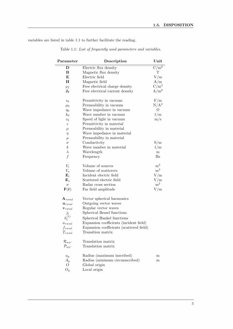
variables are listed in table 1.1 to further facilitate the reading.

Table 1.1: List of frequently used parameters and variables.

Parameter Description Unit

D Electric flux density C/m2

B Magnetic flux density TE Electric field V/mH Magnetic field A/mρf Free electrical charge density C/m3

Jf Free electrical current density A/m2

ε0 Permittivity in vacuum F/mµ0 Permeability in vacuum N/A2

η0 Wave impedance in vacuum Ωk0 Wave number in vacuum 1/mc0 Speed of light in vacuum m/sε Permittivity in materialµ Permeability in materialη Wave impedance in materialµ Permeability in materialσ Conductivity S/mk Wave number in material 1/mλ Wavelength mf Frequency Hz

Vi Volume of sources m3

Vs Volume of scatterers m3

Ei Incident electric field V/mEs Scattered electric field V/mσ Radar cross section m2

F(r) Far field amplitude V/m

Aτσml Vector spherical harmonicsuτσml Outgoing vector wavesvτσml Regular vector wavesjl Spherical Bessel functions

h(1)l Spherical Hankel functions

aτσml Expansion coefficients (incident field)fτσml Expansion coefficients (scattered field)Tτσml Transition matrix

Rnn′ Translation matrixPnn′ Translation matrix

ap Radius (maximum inscribed) mAp Radius (minimum circumscribed) mO Global originOp Local origin

3

Chapter 2

Theory

This chapter will shortly present all relevant theory for this thesis work. No derivations will beperformed, instead the main results from the theory needed will be presented here. For derivationsand more information the reader is directed to the references. The theory chapter is mainly asummary of the most relevant theory described in the book by Gerhard Kristensson [13] and forthe interested reader more information can be found there. Other important references are thearticle by the same author from which the implementation is made [9] and the article by Petersonand Strom which describes the T-matrix formulation for an arbitrary number of scatterers [8].

Since this thesis work concerns electromagnetic scattering we will start with introducingMaxwell’s equations followed by some general scattering theory. Thereafter the theory regard-ing the translation of spherical vector waves will be explained. Finally, the theory chapter willend with a section about multiple scattering.

2.1 Maxwell’s equations

Maxwell’s equations form the foundation of classical electrodynamics and describe how electricand magnetic fields are generated and altered by each other as well as by charges and currents[14]. The equations are named after the Scottish mathematical physicist James Clerk Maxwell,who published the well-known equations in 1865.

Maxwell’s equations can be expressed in several ways, both in integral and differential form andfurthermore from a microscopic and macroscopic point of view. Maxwell’s macroscopic equationsare also known as Maxwell’s equations in matter.

Maxwell’s macroscopic equations in differential form are expressed as

∇×E = −∂B∂t

(2.1)

∇×H = Jf +∂D

∂t(2.2)

∇ ·B = 0 (2.3)

∇ ·D = ρf (2.4)

where E is the electric field, H is the magnetic field, B is the magnetic flux density and D is theelectric flux density also called the displacement field. The free electrical charge density is denotedρf and the free electrical current density is denoted Jf .

The first of Maxwell’s equations, equation (2.1) is called Faraday’s law of induction, and thesecond equation, equation (2.2) is called Ampere’s law. Equation (2.3), is sometimes referred toas Gauss’s law of magnetism, but the name is not as well-known as the others. The last equation,equation (2.4), is called Gauss’s law.

2.1.1 Boundary conditions

In order to solve the differential equations one needs boundary conditions. The normal vector nis pointing from material 2 into material 1. We are assuming that all fields, E, B, D and H havefinite values on the boundary from both sides. This yields the boundary conditions as

n× (E1 −E2) = 0 (2.5)

4

2.1. MAXWELL’S EQUATIONS

n× (H1 −H2) = Js (2.6)

n · (B1 −B2) = 0 (2.7)

n · (D1 −D2) = ρs (2.8)

where the index 1 indicates the value of the fields in material 1.From equation (2.5) we have that the tangential component of the electric field is continuous

over the interface. Equation (2.6) says that the tangential component of the magnetic field isdiscontinuous. The size of the discontinuity is the surface current density Js. From the thirdequation, equation (2.7), we have that the normal component of the magnetic flux density iscontinuous and in equation (2.8) we see that the normal component of the displacement field isdiscontinuous over the interface. The size of the discontinuity is the surface charge density ρs.

In the case when material 2 is a perfect electric conductor (henceforth PEC), we have a specialcase for the boundary conditions. In material 2, the fields are zero and we have the followingequations for the boundary conditions

n×E1 = 0 (2.9)

n×H1 = Js (2.10)

n ·B1 = 0 (2.11)

n ·D1 = ρs (2.12)

2.1.2 Time harmonic Maxwell’s equations

The Fourier transform in time for the electric field E(r, t) is defined as

E(r, ω) =

∫ ∞−∞

E(r, t)eiωtdt (2.13)

with the inverse transform

E(r, t) =1

2π

∫ ∞−∞

E(r, ω)e−iωtdω. (2.14)

The Fourier transform for all the other fields are defined similarly. Applying the Fourier transformof the fields into Maxwell’s equations, equation (2.1)-(2.4), yields the time harmonic Maxwell’sequations as

∇×E(r, ω) = iωB(r, ω) (2.15)

∇×H(r, ω) = J(r, ω)− iωD(r, ω) (2.16)

∇ ·B(r, ω) = 0 (2.17)

∇ ·D(r, ω) = ρ(r, ω) (2.18)

2.1.3 Constitutive relations

The constitutive relation describes the relations between the fields and are expressed as

D = ε0E (2.19)

B = µ0H, (2.20)

where ε0 and µ0 are the permittivity and permeability in vacuum. If we assume time-harmonicfields the corresponding equations, for a linear isotropic material, are

D = ε0ε(ω)E (2.21)

B = µ0µ(ω)H, (2.22)

where ε(ω) and µ(ω) are the permittivity and permeability of the material.

5

CHAPTER 2. THEORY

2.1.4 Plane waves

The plane waves are a solution to Maxwell’s equations in a homogeneous, isotropic materialcharacterized by the permittivity ε(ω) and the permeability µ(ω) of the material. The planewaves are often used in forthcoming sections and are defined as

E(r, ω) = E0(ω)eikki·r, η0ηH(r, ω) = k×E0(ω)eikki·r, (2.23)

where E0(ω) is an arbitrary complex-valued vector and ki represents the propagation direction ofthe wave. E0(ω) and ki satisfy the relation E0(ω) · ki = 0, i.e. they are orthogonal. The wavenumber k of a material is defined as

k = k0

√ε(ω)µ(ω) (2.24)

where k0 = ω√ε0µ0 is the wave number in vacuum. The wave impedance η of a material is defined

as

η(ω) =

√µ(ω)

ε(ω)(2.25)

and in vacuum the wave impedance is

η0 =

õ0

ε0. (2.26)

From here on, the argument ω will not explicitly be written in the material properties or theelectric field in order to shorten the equations.

2.2 Scattering theory

In a homogeneous, isotropic material with properties ε and µ, a wave propagates without distur-bances. On the other hand if there is an obstacle, like a material with different material properties,the propagation of the wave will be affected. This behaviour is called scattering [13].

An example of a scattering geometry can be seen in figure 2.1, where Vi is the volume of thesources and Vs is the volume of the disturbances called the scatterers. Both volumes can consistof more than one source or scatterer.

Vi

ε µ

Vs

Figure 2.1: An example of a scattering geometry where Vi is the volume of the sources and Vs isthe volume of the scatterers.

The original, unaffected wave is called the incident wave with index i. The incident electricand magnetic fields, Ei respectively Hi, are thus∇×Ei = iωµ0µHi = ikη0ηHi

∇×Hi = −iωε0εEi = −i kη0η

Eir /∈ Vi (2.27)

6

2.2. SCATTERING THEORY

The above fields are the total fields in absence of any scatterers. If there exists a region with oneor more scatterers, a disturbance will occur in the fields. Those fields are called the scattered fieldswith index s. The scattered electric and magnetic fields are source free outside the region Vs∇×Es = iωµ0µHs = ikη0ηHs

∇×Hs = −iωε0εEs = −i kη0η

Esr /∈ Vs (2.28)

The scattered fields have their sources inside the volume Vs, which are generated by the sourcesin Vi. The total field is the summation of both fields, which for the electric field is

E = Es + Ei. (2.29)

2.2.1 Radar cross section

An important definition within the area of scattering theory is the radar cross section (henceforthRCS), which is a measure of power scattered in a given direction when an object is illuminatedby an incident wave [1]. The definition of the RCS is

σ = limr→∞

4πr2 |Es|2

|Ei|2(2.30)

where r is the distance from the scatterer to the point where the scattered power is measured,Es is the scattered electric field and Ei is the electric field incident at the object. The RCS isnormalized with the power density of the incident wave. The scattered field is |Es| ∼ 1/r, themultiplication with r2 thus makes the RCS independent of the distance r. As the name indicates,the RCS is measured in m2.

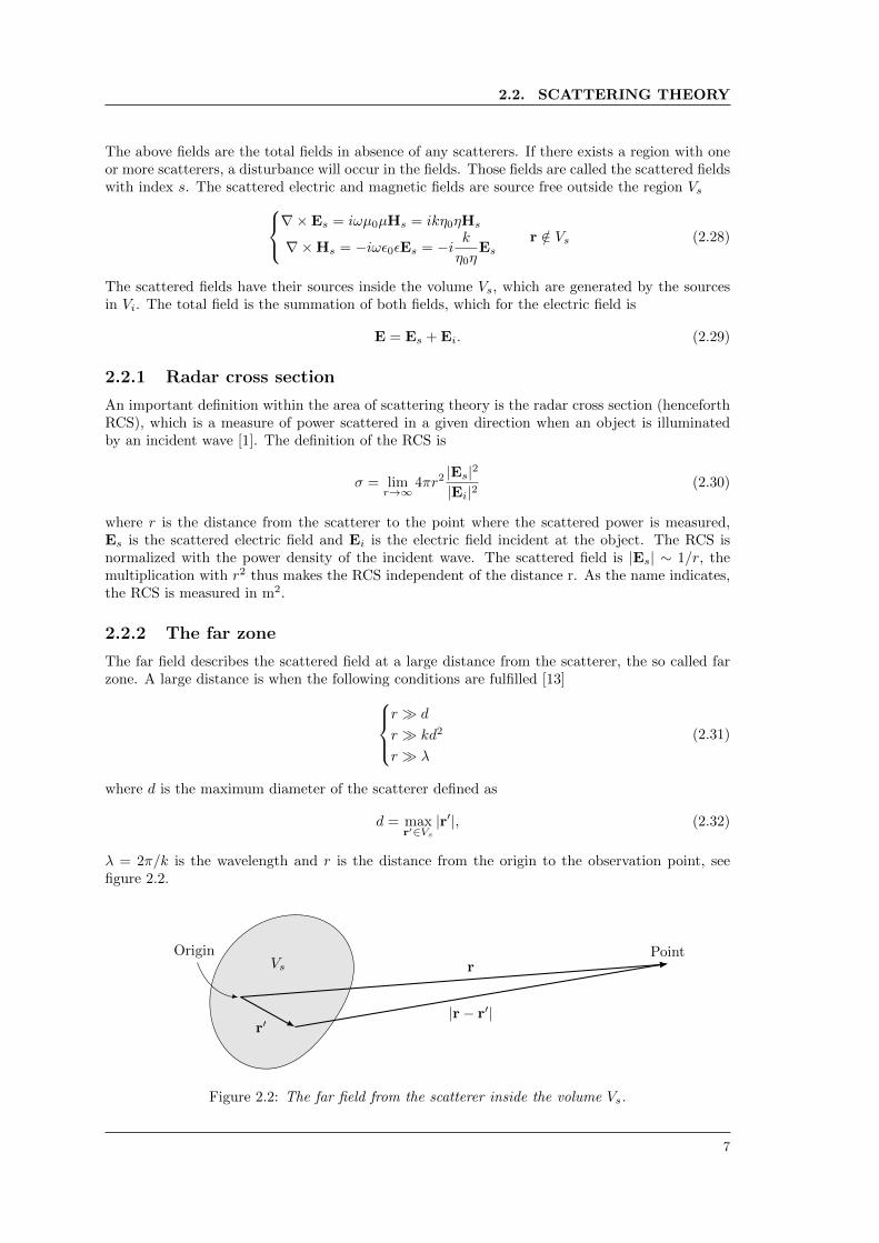
2.2.2 The far zone

The far field describes the scattered field at a large distance from the scatterer, the so called farzone. A large distance is when the following conditions are fulfilled [13]

r d

r kd2

r λ

(2.31)

where d is the maximum diameter of the scatterer defined as

d = maxr′∈Vs

|r′|, (2.32)

λ = 2π/k is the wavelength and r is the distance from the origin to the observation point, seefigure 2.2.

Vs

r′|r− r′|

rOrigin Point

Figure 2.2: The far field from the scatterer inside the volume Vs.

7

CHAPTER 2. THEORY

In the far field, the scattered electric field can be expressed as

Es(r) =eikr

krF(r), (2.33)

where F(r) is the far field amplitude defined as

F(r) = ik2

4πr×

∫∫Ss

[n(r′)×Es(r

′)− η0ηr× (n(r′)×Hs(r′))]e−ikr·r

′dS′. (2.34)

2.2.3 Helmholtz equation

In order to find solutions to Maxwell’s equations in a source free, homogeneous, isotropic material,described as ∇×E = ikη0ηH

∇×H = −i kη0η

E, (2.35)

we introduce the Helmholtz differential equation. The Helmholtz differential equation is obtainedcombining Maxwell’s equations to one by eliminating either the electric or the magnetic field. Inorder to satisfy Maxwell’s equations, the solutions should be divergence free. If we take the curlof the first equation and the divergence of the second equation using the fact that ∇ ·∇×H = 0,we have an alternative formulation as

∇2E(r) + k2E(r) = 0

∇ ·E(r) = 0. (2.36)

The first equation is called the Helmholtz differential equation.

2.2.4 Vector spherical harmonics

The solution to the Helmholtz differential equation in spherical coordinates can be expressed usingspherical vector waves, which are vector-valued functions. In order to create those vector waveswe want to define new vector-valued basis functions. Those basis functions should satisfy fourproperties listed below:

1. The basis functions should be solutions to the Helmholtz differential equation ∇2E(r) +k2E(r) = 0.

2. The basis functions, which are functions of r and r, shall when r is held fixed be completefor all a > 0.

3. There should be a simple relationship between the electric and magnetic field.

4. It should be easy to identify the subset of basis functions with divergence zero. Since theyare interesting for the solutions to Maxwell’s equations in source free areas.

The vector spherical harmonics

Aτσml(r),

τ = 1, 2, 3

σ = e, o

m = 0, 1, . . . , l − 1, l

l = 0, 1, 2, 3, . . .

(2.37)

8

2.2. SCATTERING THEORY

have the above stated criteria where σ = e, o stands for even and odd respectively. The vectorspherical harmonics A1σml(r) are defined as

A1σml(r) =1√

l(l + 1)∇× (rYσml(r)) =

1√l(l + 1)

∇Yσml(r)× r

A2σml(r) =1√

l(l + 1)r∇Yσml(r)

A3σml(r) = rYσml(r)

(2.38)

where Yσml are the spherical harmonics. A more thoroughly description can be found in appendixA. Now when we have defined our new basis functions we are ready to define the outgoing sphericalvector waves uτσml

u1σml(kr) = h(1)l (kr)A1σml(r)

u2σml(kr) =1

k∇×

(h

(1)l (kr)A1σml(r)

)u3σml(kr) =

1

k∇(h

(1)l (kr)Y1σml(r)

) (2.39)

and the regular spherical vector waves vτσml

v1σml(kr) = jl(kr)A1σml(r)

v2σml(kr) =1

k∇×

(jl(kr)A1σml(r)

)v3σml(kr) =

1

k∇(jl(kr)Y1σml(r)

) (2.40)

where h(1)l (kr) and jl(kr) are the spherical Hankel and Bessel functions respectively, which are

defined in appendix B.

2.2.5 T-matrix formulation

The T-matrix formulation, or the Null-field approach as it is also called, is used in order to findthe solution of the scattering problem. The main idea is to find the transition matrix Tnn′ , whichcontains the general solution to the problem [5], [6], [7], [8], [10], [13]. The transition matrix isfound using the Null-field theorem which is based on the surface integral representations of thefields. In this section, the equations regarding the T-matrix formulation will be presented. Thetransition matrix has given the T-matrix formulation its name.

Assuming that the incident field is a plane wave, it can be expanded in the regular sphericalvector waves vτσml(kr) as

Ei(r) = E0eikki·r =

∞∑l=0

l∑m=0

∑σ=e,o

3∑τ=1

aτσmlvτσml(kr). (2.41)

The expansion coefficients aτσml can be expressed asa1σml = 4πilE0 ·A1σml(ki)

a2σml = −4πil+1E0 ·A2σml(ki)

a3σml = −4πil+1E0 ·A3σml(ki)

. (2.42)

From the section about plane waves, section 2.1.4, we know that the plane wave need to fulfil thecondition E0(ω) · ki = 0 in order to satisfy Maxwell’s equations. This means that the complexvector E0 and the direction of the wave ki have to be orthogonal, i.e. the plane wave is divergence-free. Therefore a3σml = 0 since A3σml(ki) is proportional to ki. This means that the summationover τ will only be from 1 to 2, which implies that the summation over l starts from l = 1.

9

CHAPTER 2. THEORY

There will be no contribution from l = 0, since A1σ00(r) and A2σ00(r) are defined to be zero,see appendix A. With an incident field in the z-direction, i.e. ki = z, the expansion coefficientssimplify to

a1σml = ilδm1

√2π(2l + 1)E0 · (δσox− δσey)

a2σml = −il+1δm1

√2π(2l + 1)E0 · (δσex + δσoy)

a3σml = 0

. (2.43)

which means that only m = 1 contributes.The scattered field Es has a corresponding expansion in the outgoing spherical vector waves

outside of the circumscribing sphere of the scatterer with radius R. The expansion of the scatteredfield is

Es(r) =

∞∑l=0

l∑m=0

∑σ=e,o

2∑τ=1

fτσmluτσml(kr), r > R (2.44)

where the expansion coefficients fτσml are found using the transition matrix Tτσml,τ ′σ′m′l′ . Therelation between the expansion coefficients is linear according to

fτσml =∞∑l′=1

l′∑m′=0

∑σ′=e,o

2∑τ ′=1

Tτσml,τ ′σ′m′l′aτ ′σ′m′l′ . (2.45)

The transition matrix, Tτσml,τ ′σ′m′l′ , contains the general solution of the scattering problem. Thetotal electric field is the summation between the incident and scattered fields, which in terms ofthe spherical vector waves is

E(r) =

∞∑l=1

l∑m=0

∑σ=e,o

2∑τ=1

(aτσmlvτσml(kr) + fτσmluτσml(kr)). (2.46)

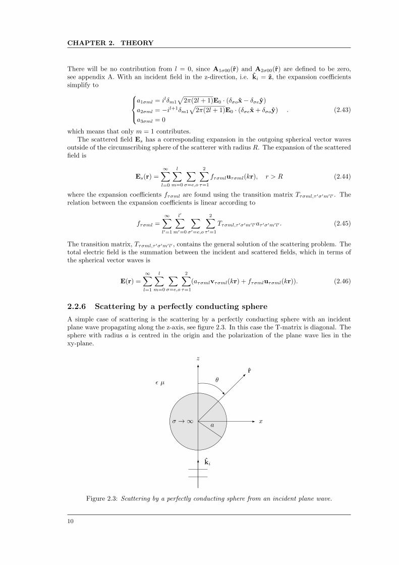
2.2.6 Scattering by a perfectly conducting sphere

A simple case of scattering is the scattering by a perfectly conducting sphere with an incidentplane wave propagating along the z-axis, see figure 2.3. In this case the T-matrix is diagonal. Thesphere with radius a is centred in the origin and the polarization of the plane wave lies in thexy-plane.

r

z

x

θ

a

ε µ

σ →∞

ki

Figure 2.3: Scattering by a perfectly conducting sphere from an incident plane wave.

10

2.3. TRANSLATION OF SPHERICAL VECTOR WAVES

Equation (2.41), (2.43) and (2.44) in section 2.2.5 define the expansion of the incident planewave in spherical vector waves, the expansions coefficients aτσml and the scattered field Es outsideof the sphere with radius a. The boundary condition on the sphere’s surface, r = a, is accordingto equation (2.9)

r×E(r)|r=a = 0. (2.47)

Since the vector spherical harmonics Aτσml are orthogonal , the above boundary condition impliesthat the expansion coefficients must satisfy

a1σmljl(ka) + f1σmlh(1)l (ka) = 0

a2σml(kajl(ka))′ + f2σml(kah(1)l (ka))′ = 0

(2.48)

The spherical Bessel and Hankel functions jl and h(1)l are independent of the indices m and σ so

we can rewrite the equation asfτσml = tτlaτσml (2.49)

where the matrix entries tτl are t1l = − jl(ka)

h(1)l (ka)

t2l = − (kajl(ka))′

(kah(1)l (ka))′

(2.50)

Once the transition entries tτl are found, the scattering problem is solved and it could be usedto calculate the radar cross section σ or the total electric field E. In this case of geometry thescattered field could be found using the far field amplitude

F(r) =

∞∑l=1

l∑m=0

∑σ=e,o

2∑τ=1

i−l−2+τfτσmlAτσml(r)

= −i∞∑l=1

√2π(2l + 1)

((E0 · x)A1o1l(r)− (E0 · y)A1e1l(r))t1l

+((E0 · x)A2e1l(r) + (E0 · y)A2o1l(r))t2l

(2.51)

where the scattered electric field is found as

Es(r) =eikr

krF(r). (2.52)

Note that only m = 1 contributes since the incident field is propagating along the z-axis.

2.3 Translation of spherical vector waves

In the multiple scattering case we have more than one scatterer. This means that the scattererswill no longer be located in the origin as in section 2.2.5 when the T-matrix formulation wasintroduced. In order to solve the multiple scattering case we therefore need to translate thespherical vector waves [9], [11], [12]. In this section the theory needed to translate the sphericalvector waves will be explained and in the following section, section 2.4, the translation will beutilized in the multiple scattering case.

In figure 2.4, the relation between the translated origins O and O′ and their correspondingposition vectors r and r′ are presented. The translation between the origins is defined as r′ − r.The spherical coordinates of r, r′ and d are defined by (r, θ, φ), (r′, θ′, φ′) and (d, η, ψ).

11

CHAPTER 2. THEORY

r

r′

d

xy

z

x′y′

z′

Figure 2.4: Translated coordinate system.

In order to improve the readability the new multi-index n = τσml is introduced, which will beused from here on. The translated spherical vector waves are expressed as [9]

vn(kr′) =1∑n′Rnn′(kd)vn′(kr), for all d

un(kr′) =1∑n′Rnn′(kd)un′(kr), r > d

un(kr′) =1∑n′Pnn′(kd)vn′(kr), r < d

(2.53)

where Rnn′ and Pnn′ are the translation matrices for a translation d (d ≥ 0). The inputs to thetranslation matrix Pnn′ are defined as

P1σml,1σm′l′(kd) = (−1)m′Cml,m′l′(d, η) cos((m−m′)ψ)

+(−1)σCml,−m′l′(d, η) cos((m+m′)ψ)

P1σml,1σ′m′l′(kd) = (−1)m′+σ′

Cml,m′l′(d, η) sin((m−m′)ψ)

+Cml,−m′l′(d, η) sin((m+m′)ψ), σ 6= σ′

P1σml,2σ′m′l′(kd) = (−1)m′+σDml,m′l′(d, η) cos((m−m′)ψ)

−Dml,−m′l′(d, η) cos((m+m′)ψ)

P1σml,2σm′l′(kd) = (−1)m′Dml,m′l′(d, η) sin((m−m′)ψ)

(−1)σDml,−m′l′(d, η) sin((m+m′)ψ)

P2σml,τσ′m′l′(kd) = P1σml,τσ′m′l′(kd), τ = 1, 2

(2.54)

where τ is the opposite to τ . The coefficients Cml,m′l′(d, η) and Dml,m′l′(d, η) are defined as

Cml,m′l′(d, η) =(−1)m+m′

2

√εmε′m

4l+l′∑

λ=|l−l′|

(−1)(l′−l+λ)/2(2λ+ 1)

√(2l + 1)(2l′ + 1)(λ− (m−m′))!l(l + 1)l′(l′ + 1)(λ+ (m−m′))!(

l l′ λ0 0 0

)(l l′ λm −m′ m′ −m

)[l(l + 1) + l′(l′ + 1)− λ(λ+ 1)]

h(1)λ (kd)Pm−m

′

λ (cos η) (2.55)

12

2.4. MULTIPLE SCATTERING

and

Dml,m′l′(d, η) =(−1)m+m′

2

√εmε′m

4l+l′∑

λ=|l−l′|+1

(−1)(l′−l+λ+1)/2(2λ+ 1)

√(2l + 1)(2l′ + 1)(λ− (m−m′))!l(l + 1)l′(l′ + 1)(λ+ (m−m′))!(

l l′ λ− 10 0 0

)(l l′ λm −m′ m′ −m

)√λ2 − (l − l′)2

√(l + l′ + 1)2 − λ2

h(1)λ (kd)Pm−m

′

λ (cos η) (2.56)

In the above equations we have that εm = 2− δm,0 is the Neumann factor, that

(· · ·· · ·

)denotes

the Wigner’s 3j symbol [15] and that

(−1)σ =

1, σ = e

−1, σ = o. (2.57)

The difference between the translation matrices Rnn′ and Pnn′ is that in Rnn′ the spherical

Hankel function h(1)λ (kd) is replaced with the spherical Bessel function jλ(kd). A useful quantity

is that the translation in the opposite direction is identical to the transpose of the translationmatrices

RT (kd) = R(−kd), PT (kd) = P(−kd). (2.58)

2.4 Multiple scattering

In this section we will go through the theory regarding the T-matrix formulation for a collectionof scatterers [7], [9], [10]. The difference between the T-matrix formulation described in section2.2.5 for one scatterer is that in that case, only one scatterer is present in the origin. With morethan one scatterer they are distributed over a larger volume. The theory described here basicallyfollows the one described in [9].

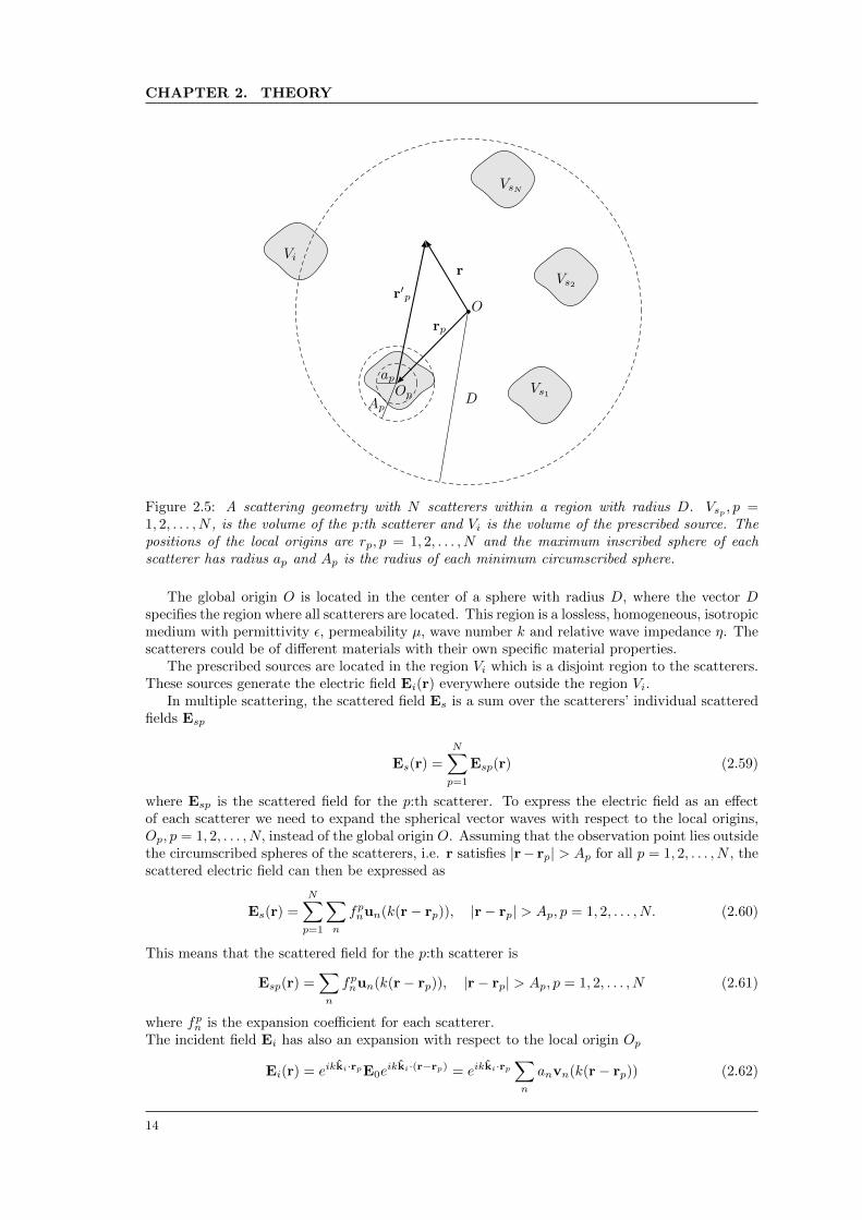
In multiple scattering we study a collection of N different scatterers, where each scatterer hasits center located in the local origin Op, p = 1, 2, . . . , N . The local origins are specified with theposition vector rp, which is the vector pointing from the global origin O, see figure 2.5. The shapeof each scatterer could be different but all scatterers have one maximum inscribed sphere withradius ap and one minimum circumscribed sphere with radius Ap. The spheres with radius ap andAp are both centred in the local origin Op, p = 1, 2, . . . , N . An important assumption is that noneof these spheres intersect with the other scatterers.

13

CHAPTER 2. THEORY

D

O

r

r′p

rp

ap

ApOp Vs1

Vs2

VsN

Vi

Figure 2.5: A scattering geometry with N scatterers within a region with radius D. Vsp , p =1, 2, . . . , N , is the volume of the p:th scatterer and Vi is the volume of the prescribed source. Thepositions of the local origins are rp, p = 1, 2, . . . , N and the maximum inscribed sphere of eachscatterer has radius ap and Ap is the radius of each minimum circumscribed sphere.

The global origin O is located in the center of a sphere with radius D, where the vector Dspecifies the region where all scatterers are located. This region is a lossless, homogeneous, isotropicmedium with permittivity ε, permeability µ, wave number k and relative wave impedance η. Thescatterers could be of different materials with their own specific material properties.

The prescribed sources are located in the region Vi which is a disjoint region to the scatterers.These sources generate the electric field Ei(r) everywhere outside the region Vi.

In multiple scattering, the scattered field Es is a sum over the scatterers’ individual scatteredfields Esp

Es(r) =

N∑p=1

Esp(r) (2.59)

where Esp is the scattered field for the p:th scatterer. To express the electric field as an effectof each scatterer we need to expand the spherical vector waves with respect to the local origins,Op, p = 1, 2, . . . , N, instead of the global origin O. Assuming that the observation point lies outsidethe circumscribed spheres of the scatterers, i.e. r satisfies |r− rp| > Ap for all p = 1, 2, . . . , N , thescattered electric field can then be expressed as

Es(r) =

N∑p=1

∑n

fpnun(k(r− rp)), |r− rp| > Ap, p = 1, 2, . . . , N. (2.60)

This means that the scattered field for the p:th scatterer is

Esp(r) =∑n

fpnun(k(r− rp)), |r− rp| > Ap, p = 1, 2, . . . , N (2.61)

where fpn is the expansion coefficient for each scatterer.The incident field Ei has also an expansion with respect to the local origin Op

Ei(r) = eikki·rpE0eikki·(r−rp) = eikki·rp

∑n

anvn(k(r− rp)) (2.62)

14

2.4. MULTIPLE SCATTERING

which is a simple translation of the origin of the incident plane wave. For an observation pointinside the inscribed sphere of the p:th scatterer, i.e. |r−rp| < ap, we have that the incident electricfield is

Ei(r) =∑n

αpnvn(k((r− rp))−N∑q=1q 6=p

∑n

fqnun(k(r− rp)), |r− rp| < ap (2.63)

for p = 1, 2, · · · , N and where the first term is the exciting field at the position of the scattererlocated at rp. Rewriting equation (2.63) may facilitate the physical interpretation. We have that

Eexcp(r) =∑n

αpnvn(k(r− rp)) = Ei(r) +

N∑q=1q 6=p

Esq(r), |r− rp| < ap (2.64)

which means that the exciting field Eexcp at the scatterer located at rp consists of the incidentfield plus all scattered fields from the scatterers except the contribution from the p:th scatterer.

In order to find a relation between the unknown coefficients of fpn and the expansion coefficientsαpn, we need coordinates referring to the same origin, in this case the local origin Op. Using thetranslation properties of the spherical vector waves in section 2.3 we have the relation

un(k(r− rq)) = un(k(r− rp)) + (k(rp − rq)) =∑n′

Pnn′(k(rp − rq))vn′(k(r− rp)), |r− rp| < |rp − rq|, (2.65)

where Pnn′ is calculated according to equation (2.54). Inserting equation (2.61) in equation (2.64)and using equation (2.65) together with the orthogonality of the vector spherical harmonics wehave that the expansion coefficients αpn can be expressed as

αpn = eikki·rpan +

N∑q=1q 6=p

∑n′

fpn′Pn′n(k(rp − rq)), p = 1, 2, . . . , N (2.66)

The expansion coefficients fpn and αpn have a relation through the transition matrix T pnn′ for thep:th scatterer as

fpn =∑n′

T pnn′αpn′ , p = 1, 2, . . . , N. (2.67)

The expansion coefficients of the scattered field, fpn are expressed as the outgoing spherical vectorwaves un(kr) and the expansion coefficients of the local excitation αpn in terms of regular sphericalvector waves vn(kr), both at the local origin rp.

Using the relation Pn′n(−kr) = Pnn′(kr) and equation (2.67), equation (2.66) can be expressedas

αpn = eikki·rpan +

N∑q=1q 6=p

∑n′n′′

Pnn′(k(rq − rp))Tqn′n′′α

qn′′ , p = 1, 2, . . . , N (2.68)

Multiplying equation (2.68) with T pnn′ followed by a summation over the free index the expansioncoefficients are found as

fpn = eikki·rp∑n′

T pnn′an′ +

N∑q=1q 6=p

∑n′n′′

T pnn′Pn′n′′(k(rq − rp))fqn′′ (2.69)

The above relation between the unknown expansion coefficients fpn is all we need to solve themultiple scattering case. Once the expansion coefficients fpn are known, the scattered field can befound according to equation (2.60).

15

CHAPTER 2. THEORY

The coefficients of the scattered field by the entire collection of scatterers fn, can be expressedin terms of the local scatterers’ expansion coefficients fpn. Using equation (2.60) and the translationproperties defined in section 2.3 we have

Es(r) =

N∑p=1

Esp(r) =

N∑p=1

∑n

fpnun(k(r− rp)) (2.70)

2.4.1 Multiple scattering by two spheres

The above theory is a general case with N scatterers. In this thesis we are interested in the specialcase of two scatterers, N = 2, which is the simplest multiple scattering case. In the case with twoscatterers, equation (2.69) is simplified to

f1n = eikki·r1

∑n′T 1nn′an′ +

∑n′n′′

T 1nn′Pn′n′′(k(r2 − r1))f2

n′′

f2n = eikki·r2

∑n′T 2nn′an′ +

∑n′n′′

T 2nn′Pn′n′′(k(r1 − r2))f1

n′′(2.71)

which in matrix notation isf1 = eikki·r1T 1a+ T 1P(k(r2 − r1))f2

f2 = eikki·r2T 2a+ T 2PT (k(r2 − r1))f1(2.72)

with the solutionf1 = (I − T 1P(k(r2 − r1))T 2PT (k(r2 − r1)))−1

(eikki·r1T 1 + eikki·r2T 1P(k(r2 − r1))T 2

)a

f2 = eikki·r2T 2a+ T 2PT (k(r2 − r1))f1

(2.73)where I is the identity matrix. Note that the superscript 2 on T and f denotes the appropriatescatterer and not the square of the element.

16

Chapter 3

Methodology

In this chapter we will go through all implementation steps performed in order to succeed in thegoal of implementing multiple scattering by two spheres. The implementation of this thesis workwas divided into five steps, which are further described in section 3.1. Each step was performedto validate a new part of the implementation.

Furthermore, this chapter describes the improvements made to the original implementation,which was applied in order to translate the spheres further apart.

3.1 Implementation

As mentioned earlier, the implementation is divided into five steps. In each step a new part of thetheory is included. The implementation will start with expressing the incident field in sphericalvector waves, advance through translated, spherical vector waves and finally end with a sectionabout the multiple scattering by two spheres.

In the first step of the implementation, the regular spherical vector waves are implemented andvisualized. Secondly, the scattered field around a PEC is implemented to validate the outgoingspherical vector waves, scattered from the incident wave. In the third step, the regular sphericalvector waves are translated in the z-direction. This step is performed to validate the implementa-tion of the translation matrix R. In the fourth step, the translation matrix R is used to convertthe expansion coefficients fn to new ones, which are needed in order to calculate the translated,outgoing spherical vector waves. Lastly, the translation matrix R is changed to P by altering the

spherical Bessel functions jl to spherical Hankel functions h(1)l . In this step the multiple scattering

case is implemented.A figurative sketch over the implementation procedure can be seen in figure 3.1.

Incidentfield

Scatteredfield

Translatedincident

field

Translatedscattered

field

Multiplescattering

Figure 3.1: Schematic picture over the implementation procedure.

All implementations have been made using MATLAB, MathWorks R2013b. Every step in theimplementation consists of the implementation made in earlier stages. Throughout the wholeimplementation we will consider perfectly conducting spheres translated along the z-axis with anincident field along the z-axis.

3.1.1 Incident field

In the absolute first step of the implementation we will investigate the case with no scatteringand only look at the incident field in order to correctly implement the vector spherical harmonicsAn, the spherical regular vector waves vn and the corresponding expansion coefficients an. Tostart with, the size of the xz-plane and the frequency f are specified. The wave number k isimplemented as k = 2πf/c, where c is the speed of light. The length of the position vector r isdefined as

r =√x2 + y2 + z2. (3.1)

17

CHAPTER 3. METHODOLOGY

The polarization of the field is specified asE0x = E

‖0 = cosα

E0y = E⊥0 = sinα(3.2)

where α equals zero results in a polarization parallel to the plane and α = π/2 results in apolarization perpendicular to the plane.

Since we are interested in the incident electric field described in equation (2.41) expressed as aninfinite sum we need to find a lmax which truncates after a finite number in the implementation.In this case, with plane waves at a plane, we use a ”sufficiently high” value, meaning that wechoose a lmax which will give an accurate result. The value of lmax is chosen to be proportionalto kr.

Since we have the incident field along the z-axis, the summation index m = 1, which simplifiesthe implementation. For each l, the Legendre polynomials Pl, the spherical Bessel function jl andboth their derivatives are calculated using the built-in functions in MATLAB, named legendre()

and besselj().Both the even and odd versions of the θ-, φ- and r-component of the vector spherical harmonics

An are then found according to equation (A.10). Since m = 1, the Legendre functions, equation(A.4) simplifies to

P 1l (cos θ) = sin θ

d

d(cos θ)Pl(cos θ). (3.3)

where Pl is the Legendre polynomial. We also have that ε = 2 which, together with equation (3.3),simplifies the spherical harmonics to

Yσ1l(θ, φ) =

√1

π

√2l + 1

2

(l − 1)!

(l + 1)!P 1l (cos θ)

cosφsinφ

=

√1

2π

√(2l + 1)

l(l + 1)sin(θ)P ′l (cos θ)

cosφsinφ

.

(3.4)

The expansion coefficients an are calculated according to equation (2.43). The regular vectorwaves vn are calculated according to equation (2.40) and finally the incident field is calculatedfrom equation (2.41). The components of the field are implemented in spherical coordinates andthen converted to Cartesian before visualised.

3.1.2 Scattered field

The aim with this sub problem is, in an early stage, to validate the elementary scattering theorydescribed in section 2.2. In this step we will add the outgoing spherical vector waves un, thetransition matrix Tnn′ as well as the expansion coefficients fn. In addition to the above stateddefinitions we define the radius of the sphere a.

In the case when we have scattering by a sphere there exist several ways of how the lmax shouldbe determined. Many sources have used formulas to calculate the lmax depending on the radius ofthe sphere [16], [17]. We have chosen to use a convergence test in order to find the value of lmaxby considering the l dependence of the relative error [18]

ε(l) =|Ul − U ||U |

(3.5)

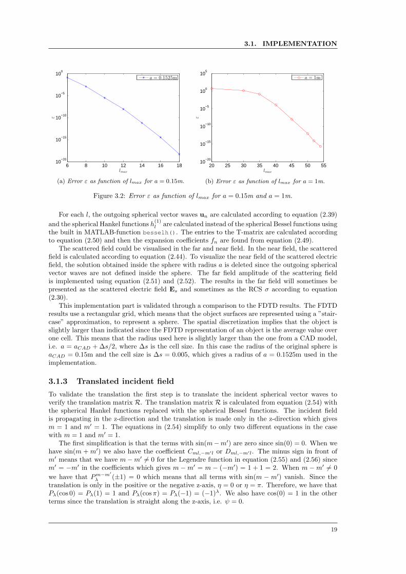
where Ul is the truncated series and U is the converged value, which is calculated for a sufficientlylarge l. In figure 3.2 the error ε is plotted as a function of lmax for radius a = 0.15m and a = 1min figure 3.2a and 3.2b respectively. For an error about 10−10 one should use lmax between 12and 14 for a = 0.15m and between 45 and 50 for a = 1m. Note that the lmax is larger for largerradiuses of the sphere as predicted in [16], [17].

18

3.1. IMPLEMENTATION

6 8 10 12 14 16 1810

−20

10−15

10−10

10−5

100

lmax

ε

a = 0.1525m

(a) Error ε as function of lmax for a = 0.15m.

20 25 30 35 40 45 50 5510

−20

10−15

10−10

10−5

100

105

lmax

ε

a = 1m

(b) Error ε as function of lmax for a = 1m.

Figure 3.2: Error ε as function of lmax for a = 0.15m and a = 1m.

For each l, the outgoing spherical vector waves un are calculated according to equation (2.39)

and the spherical Hankel functions h(1)l are calculated instead of the spherical Bessel functions using

the built in MATLAB-function besselh(). The entries to the T-matrix are calculated accordingto equation (2.50) and then the expansion coefficients fn are found from equation (2.49).

The scattered field could be visualised in the far and near field. In the near field, the scatteredfield is calculated according to equation (2.44). To visualize the near field of the scattered electricfield, the solution obtained inside the sphere with radius a is deleted since the outgoing sphericalvector waves are not defined inside the sphere. The far field amplitude of the scattering fieldis implemented using equation (2.51) and (2.52). The results in the far field will sometimes bepresented as the scattered electric field Es and sometimes as the RCS σ according to equation(2.30).

This implementation part is validated through a comparison to the FDTD results. The FDTDresults use a rectangular grid, which means that the object surfaces are represented using a ”stair-case” approximation, to represent a sphere. The spatial discretization implies that the object isslightly larger than indicated since the FDTD representation of an object is the average value overone cell. This means that the radius used here is slightly larger than the one from a CAD model,i.e. a = aCAD + ∆s/2, where ∆s is the cell size. In this case the radius of the original sphere isaCAD = 0.15m and the cell size is ∆s = 0.005, which gives a radius of a = 0.1525m used in theimplementation.

3.1.3 Translated incident field

To validate the translation the first step is to translate the incident spherical vector waves toverify the translation matrix R. The translation matrix R is calculated from equation (2.54) withthe spherical Hankel functions replaced with the spherical Bessel functions. The incident fieldis propagating in the z-direction and the translation is made only in the z-direction which givesm = 1 and m′ = 1. The equations in (2.54) simplify to only two different equations in the casewith m = 1 and m′ = 1.

The first simplification is that the terms with sin(m−m′) are zero since sin(0) = 0. When wehave sin(m + m′) we also have the coefficient Cml,−m′l or Dml,−m′l. The minus sign in front ofm′ means that we have m−m′ 6= 0 for the Legendre function in equation (2.55) and (2.56) sincem′ = −m′ in the coefficients which gives m −m′ = m − (−m′) = 1 + 1 = 2. When m −m′ 6= 0

we have that Pm−m′

λ (±1) = 0 which means that all terms with sin(m − m′) vanish. Since thetranslation is only in the positive or the negative z-axis, η = 0 or η = π. Therefore, we have thatPλ(cos 0) = Pλ(1) = 1 and Pλ(cosπ) = Pλ(−1) = (−1)λ. We also have cos(0) = 1 in the otherterms since the translation is straight along the z-axis, i.e. ψ = 0.

19

CHAPTER 3. METHODOLOGY

The R-matrix is constructed as

Rll′ =

−Cll′ −Dll′ 0ll′ 0ll′

Dll′ −Cll′ 0ll′ 0ll′

0ll′ 0ll′ −Cll′ Dll′

0ll′ 0ll′ −Dll′ −Cll′

(3.6)

where Cll′ and Dll′ are lmax × lmax-matrices and 0ll′ is a zero-matrix with size lmax × lmax.The coefficients C and D, defined in equation (2.55) and (2.56), are with the above describedsimplifications implemented as

Cml,m′l′(d, η) =

l+l′∑λ=|l−l′|

1

2(−1)(l′−l+λ)/2(2λ+ 1)

√(2l + 1)(2l′ + 1)

l(l + 1)l′(l′ + 1)

(l l′ λ0 0 0

)(l l′ λ1 −1 0

)[l(l + 1) + l′(l′ + 1)− λ(λ+ 1)]jλ(kd)γλ (3.7)

and

Dml,m′l′(d, η) =

l+l′∑λ=|l−l′|+1

1

2(−1)(l′−l+λ+1)/2(2λ+ 1)

√(2l + 1)(2l′ + 1)

l(l + 1)l′(l′ + 1)

(l l′ λ− 10 0 0

)(l l′ λ1 −1 0

)√λ2 − (l − l′)2

√(l + l′ + 1)2 − λ2jλ(kd)γλ (3.8)

where γ = 1 if the translation is made downwards (η = 0) and γ = −1 if the translation is madeupwards (η = π). The Wigner symbols are implemented according to [21].

A check is made to investigate the relation described in equation (2.58) to validate the imple-mentation of the translation matrix R.

The new, translated vector waves are calculated as a multiplication between the old sphericalvector waves and the validated translation matrix according to equation (2.53). The original,untranslated incident field is then found as the translated field multiplied with a phase factor as

Ei = EiT e−ikd (3.9)

where EiT is the translated field and d is the distance of the translation.

3.1.4 Translated scattered field

The implementation case with translated scattering by a sphere is very similar to the case withtranslated incident vector waves. The translated scattered field is implemented as

Es(r) =∑n

∑n′

fnRn′n(−krp)un(kr) (3.10)

where fn is the expansion coefficient calculated in the local origin of the scatterer and translatedto the global origin with Rn′n. The multiplication between fn and Rn′n represents the expansioncoefficients in the global origin which is multiplied with the spherical vector waves un.

The reference solution is translated as

Es = e−idkeikd cos θEsref . (3.11)

The term eikd cos θ is thereby comparable with the translation matrix R and since we are interestedin validating the translation matrix we use both implementations.

20

3.2. IMPROVEMENTS

3.1.5 Multiple scattering

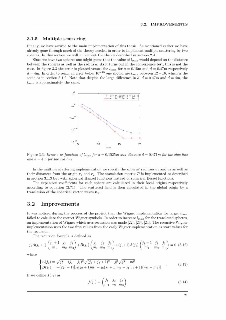
Finally, we have arrived to the main implementation of this thesis. As mentioned earlier we havealready gone through much of the theory needed in order to implement multiple scattering by twospheres. In this section we will implement the theory described in section 2.4.

Since we have two spheres one might guess that the value of lmax would depend on the distancebetween the spheres as well as the radius a. As it turns out in the convergence test, this is not thecase. In figure 3.3 the error is plotted versus the lmax for a = 0.15m and d = 0.47m respectivelyd = 4m. In order to reach an error below 10−10 one should use lmax between 12− 16, which is thesame as in section 3.1.2. Note that despite the large difference in d, d = 0.47m and d = 4m, thelmax is approximately the same.

5 10 15 2010

−15

10−10

10−5

100

105

lmax

ε

a = 0.1525m,d = 0.47ma = 0.1525m,d = 4m

Figure 3.3: Error ε as function of lmax for a = 0.1525m and distance d = 0.471m for the blue lineand d = 4m for the red line.

In the multiple scattering implementation we specify the spheres’ radiuses a1 and a2 as well astheir distances from the origin r1 and r2. The translation matrix P is implemented as describedin section 3.1.3 but with spherical Hankel functions instead of spherical Bessel functions.

The expansion coefficients for each sphere are calculated in their local origins respectivelyaccording to equation (2.71). The scattered field is then calculated in the global origin by atranslation of the spherical vector waves un.

3.2 Improvements

It was noticed during the process of the project that the Wigner implementation for larger lmaxfailed to calculate the correct Wigner symbols. In order to increase lmax for the translated spheres,an implementation of Wigner which uses recursion was made [22], [23], [24]. The recursive Wignerimplementation uses the two first values from the early Wigner implementation as start values forthe recursion.

The recursion formula is defined as

j1A(j1+1)

(j1 + 1 j2 j3m1 m2 m3

)+B(j1)

(j1 j2 j3m1 m2 m3

)+(j1+1)A(j1)

(j1 − 1 j2 j3m1 m2 m3

)= 0 (3.12)

where A(j1) =

√j21 − (j2 − j3)2

√(j2 + j3 + 1)2 − j2

1

√j21 −m2

1

B(j1) = −(2j1 + 1)[j2(j2 + 1)m1 − j3(j3 + 1)m1 − j1(j1 + 1)(m3 −m2)]. (3.13)

If we define f(j1) as

f(j1) =

(j1 j2 j3m1 m2 m3

)(3.14)

21

CHAPTER 3. METHODOLOGY

we have that

j1A(j1 + 1)f(j1 + 1) +B(j1)f(j1) + (j1 + 1)A(j1)f(j1 − 1) = 0. (3.15)

Rewriting equation (3.15) we have the recursion formula as

f(j1 + 1) = − 1

j1A(j1 + 1)

[B(j1)f(j1) + (j1 + 1)A(j1)f(j1 − 1)

](3.16)

where f(j1) and f(j1 − 1) are found using the originally used Wigner implementation [21]. TheWigner symbols obtained from the recursion are validated against the Wigner symbols at Wolframalpha [25].

22

Chapter 4

Results

In this chapter the results from the different implementation steps described in chapter 3 will bepresented. In every step a large number of results could have been presented but a selection ofthe most relevant and representative results is shown. By altering the frequency, the polarizationor the distance between the spheres different results could be achieved. All results are presentedin the xz-plane for simplicity even though many scattering planes have been validated.

When calculating the near field, colourful figures will be used to visualize the results andsometimes compared to the corresponding figures from the FDTD results. As for the far fieldboth the RCS σ and the scattered electric field Es will be presented. In that case one couldstudy both the imaginary and the real part of the solution. In early stages of the implementation,the results from the T-matrix formulation are compared to an implementation solving the Mie-scattering case, from here one referred to as reference solution, described in [1]. In the case withmultiple scattering the results will be compared with the results from the FDTD results.

The results in section 4.1-4.4 are mostly in order to validate the implementation. The mainresult is presented in the section about multiple scattering, section 4.5.

4.1 Incident field

Implementing the incident electric field Ei, as described in section 3.1.1, yields the results shownin figure 4.1. Figure 4.1a, with lmax = 45, shows the incident electric field, expressed as regularspherical vector waves, as constant phase lines. Lowering the value of lmax to 30 yields the resultsshown in figure 4.1b, showing that a lower lmax than acceptable gives the wrong results at theedges, creating a circle shaped figure in the incident field. The polarization of the incident wavewas in this implementation parallel to the plane of incidence.

x [m]

z[m

]

−1 −0.5 0 0.5 1−1

−0.5

0

0.5

1

−0.8

−0.6

−0.4

−0.2

0

0.2

0.4

0.6

0.8

(a) Incident field for lmax = 45.

x [m]

z[m

]

−1 −0.5 0 0.5 1−1

−0.5

0

0.5

1

−1

−0.5

0

0.5

1

(b) Incident field for lmax = 30.

Figure 4.1: ReEi for lmax = 45 in the left figure and the significantly lower lmax = 30 in theright figure.

23

CHAPTER 4. RESULTS

4.2 Scattered field

The near and far field figures from the implementation described in section 3.1.2 are presented inthe following section. The near field for the scattering case by one sphere is shown in figure 4.2-4.4.In the left and right figure, 4.2a and 4.2b in figure 4.2, the x- and z-component of the scatterednear field Esx and Esz are shown for frequency f = 1.5GHz and with polarization parallel to theplane of incidence.

In figure 4.3, the magnitude of the scattered electric field Es for frequency f = 1.5GHz andpolarization parallel to the plane is presented. The T-matrix implementation is shown in the leftfigure and in the right the FDTD results are presented, see figure 4.3a respectively 4.3b. Figure4.4 shows the corresponding results for the polarization perpendicular to the plane of incidence.Once again, the left figure 4.4a shows the T-matrix formulation and the right figure 4.4b showsthe FDTD results. The radius of the spheres is a = 0.1525m. The resolution in the FDTD resultsis 40 cells/wavelength, which yields sufficiently reliable results for validation purposes.

x [m]

z[m

]

−0.4 −0.2 0 0.2 0.4

−0.4

−0.2

0

0.2

0.4

−1

−0.5

0

0.5

1

(a) The scattered field Esx at 1.5GHz.

x [m]

z[m

]

−0.4 −0.2 0 0.2 0.4

−0.4

−0.2

0

0.2

0.4

−1

−0.5

0

0.5

1

(b) The scattered field Esz at 1.5GHz.

Figure 4.2: The x- and z-component of the scattered field for frequency f = 1.5 GHz and polarizationparallel to the plane of incidence.

x [m]

z[m

]

−0.4 −0.2 0 0.2 0.4

−0.4

−0.2

0

0.2

0.4

0

0.5

1

1.5

2

(a) |ReEs| at 1.5 GHz.

x [m]

z[m

]

−0.4 −0.2 0 0.2 0.4

−0.4

−0.2

0

0.2

0.4

0

0.5

1

1.5

2

(b) |ReEs| for FDTD at 1.5GHz.

Figure 4.3: Magnitude of the scattered field for the T-matrix formulation with a comparison to theFDTD results. Ei parallel to the plane of incidence.

24

4.3. TRANSLATED INCIDENT FIELD

x [m]

z[m

]

−0.4 −0.2 0 0.2 0.4

−0.4

−0.2

0

0.2

0.4

0

0.5

1

1.5

(a) |ReEs| at 1.5GHz.

x [m]

z[m

]

−0.4 −0.2 0 0.2 0.4

−0.4

−0.2

0

0.2

0.4

0

0.5

1

1.5

(b) |ReEs| for FDTD at 1.5GHz.

Figure 4.4: Magnitude of the scattered field for the T-matrix formulation with a comparison to theFDTD results. Ei perpendicular to the plane of incidence.

In figure 4.5 the RCS as a function of the angle θ for both polarizations are shown. In figure4.5a, the polarization is parallel to the plane of incidence which results in σ‖. In figure 4.5b, σ⊥ isshown since the incident wave has a polarization perpendicular to the plane of incidence. Note thatthe graphs for the T-matrix formulation and the reference solution are almost indistinguishable.Both spheres, used for the T-matrix formulation and the reference solution, have a radius ofa = 0.1525m.

0 20 40 60 80 100 120 140 160 180

10−2

10−1

100

θ[]

σ‖

[

m2]

σ‖ - T-matrix formulationσ‖ - Reference (Mie)

(a) RCS σ‖ plotted as a function of θ.

0 20 40 60 80 100 120 140 160 180

10−1

100

θ []

σ⊥

[

m2]

σ⊥ - T-matrix formulationσ⊥ - Reference (Mie)

(b) RCS σ⊥ plotted as a function of θ.

Figure 4.5: The radar cross section σ plotted as a function of the angle θ. In the left figureσ‖ is plotted for a polarization parallel to the plane of incidence and in the right figure σ⊥ isplotted for a polarization perpendicular to the plane of incidence. Both figures show a comparisonbetween the T-matrix formulation and the reference solution. Note that those graphs are almostindistinguishable.

4.3 Translated incident field

Implementing the translated, regular spherical vector waves yields the incident electric field Eishown in figure 4.6. As described in section 3.1.3 the incident waves are calculated a distanced = 0.47m down from the original origin and then translated up again. Note that the resultingimage is exactly the same as figure 4.1a where the untranslated incident field with polarizationparallel to the plane of incidence is shown.

25

CHAPTER 4. RESULTS

x [m]

z[m

]

−1 −0.5 0 0.5 1−1

−0.5

0

0.5

1

−0.8

−0.6

−0.4

−0.2

0

0.2

0.4

0.6

0.8

Figure 4.6: The real part of the translated incident field, ReEi.

4.4 Translated scattered field

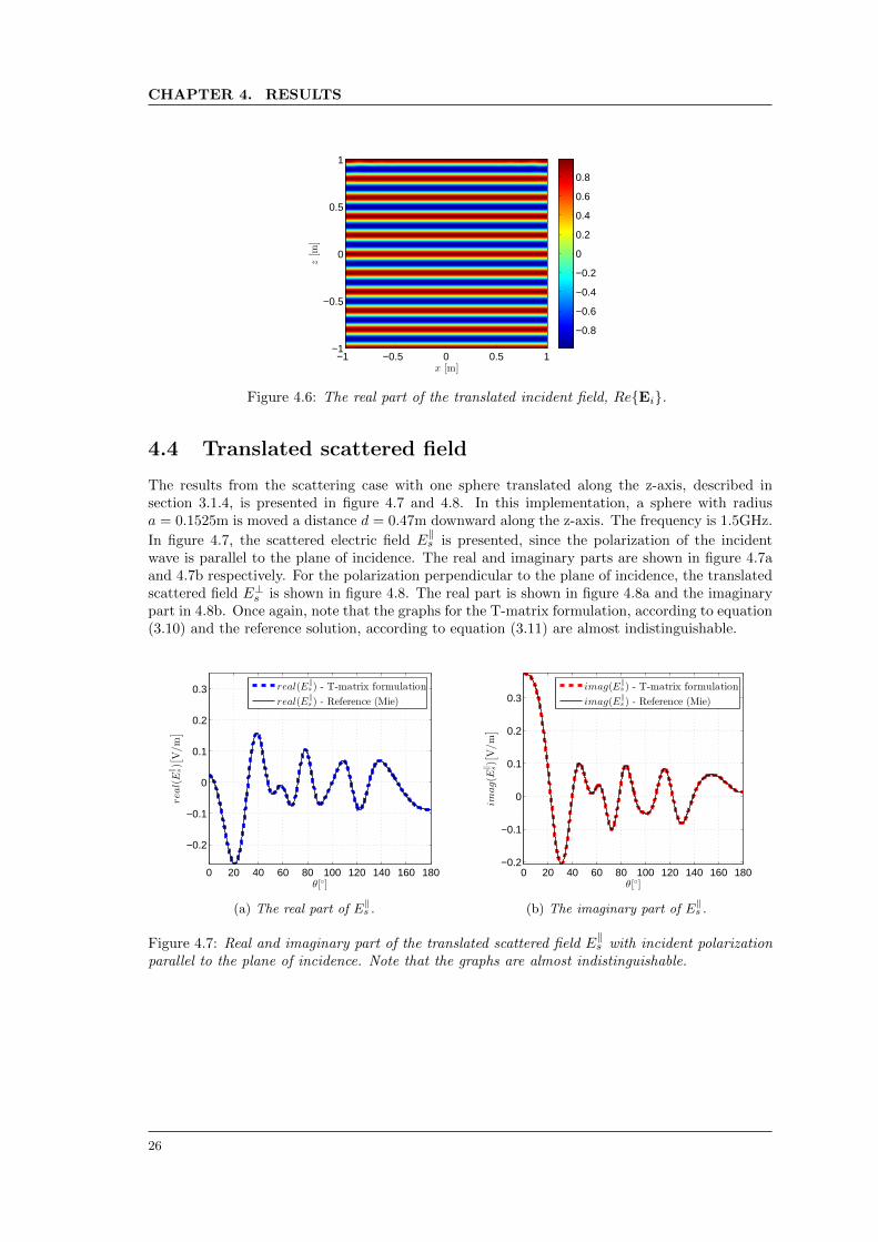
The results from the scattering case with one sphere translated along the z-axis, described insection 3.1.4, is presented in figure 4.7 and 4.8. In this implementation, a sphere with radiusa = 0.1525m is moved a distance d = 0.47m downward along the z-axis. The frequency is 1.5GHz.

In figure 4.7, the scattered electric field E‖s is presented, since the polarization of the incident

wave is parallel to the plane of incidence. The real and imaginary parts are shown in figure 4.7aand 4.7b respectively. For the polarization perpendicular to the plane of incidence, the translatedscattered field E⊥s is shown in figure 4.8. The real part is shown in figure 4.8a and the imaginarypart in 4.8b. Once again, note that the graphs for the T-matrix formulation, according to equation(3.10) and the reference solution, according to equation (3.11) are almost indistinguishable.

0 20 40 60 80 100 120 140 160 180

−0.2

−0.1

0

0.1

0.2

0.3

θ[]

real(E

‖ s)[

V/m]

real(E‖s ) - T-matrix formulation

real(E‖s ) - Reference (Mie)

(a) The real part of E‖s .

0 20 40 60 80 100 120 140 160 180−0.2

−0.1

0

0.1

0.2

0.3

θ[]

imag(E

‖ s)[

V/m]

imag(E‖s ) - T-matrix formulation

imag(E‖s ) - Reference (Mie)

(b) The imaginary part of E‖s .

Figure 4.7: Real and imaginary part of the translated scattered field E‖s with incident polarization

parallel to the plane of incidence. Note that the graphs are almost indistinguishable.

26

4.5. MULTIPLE SCATTERING

0 20 40 60 80 100 120 140 160 180

−0.1

0

0.1

0.2

θ[]

real(E

⊥ s)[

V/m]

real(E⊥

s) - T-matrix formulation

real(E⊥

s) - Reference (Mie)

(a) The real part of E⊥s .

0 20 40 60 80 100 120 140 160 180

0

0.1

0.2

0.3

θ[]

imag(E

⊥ s)[

V/m]

imag(E⊥

s ) - T-matrix formulation

imag(E⊥

s ) - Reference (Mie)

(b) The imaginary part of E⊥s .

Figure 4.8: Real and imaginary part of the translated scattered field E⊥s with incident polarizationperpendicular to the plane of incidence. Note that the graphs are almost indistinguishable.

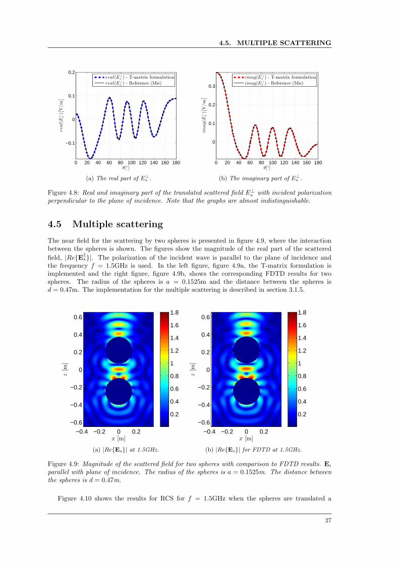
4.5 Multiple scattering

The near field for the scattering by two spheres is presented in figure 4.9, where the interactionbetween the spheres is shown. The figures show the magnitude of the real part of the scattered

field, |ReE‖s|. The polarization of the incident wave is parallel to the plane of incidence andthe frequency f = 1.5GHz is used. In the left figure, figure 4.9a, the T-matrix formulation isimplemented and the right figure, figure 4.9b, shows the corresponding FDTD results for twospheres. The radius of the spheres is a = 0.1525m and the distance between the spheres isd = 0.47m. The implementation for the multiple scattering is described in section 3.1.5.

x [m]

z[m

]

−0.4 −0.2 0 0.2

−0.6

−0.4

−0.2

0

0.2

0.4

0.6

0.2

0.4

0.6

0.8

1

1.2

1.4

1.6

1.8

(a) |ReEs| at 1.5GHz.

x [m]

z[m

]

−0.4 −0.2 0 0.2

−0.6

−0.4

−0.2

0

0.2

0.4

0.6

0.2

0.4

0.6

0.8

1

1.2

1.4

1.6

1.8

(b) |ReEs| for FDTD at 1.5GHz.

Figure 4.9: Magnitude of the scattered field for two spheres with comparison to FDTD results. Eiparallel with plane of incidence. The radius of the spheres is a = 0.1525m. The distance betweenthe spheres is d = 0.47m.

Figure 4.10 shows the results for RCS for f = 1.5GHz when the spheres are translated a

27

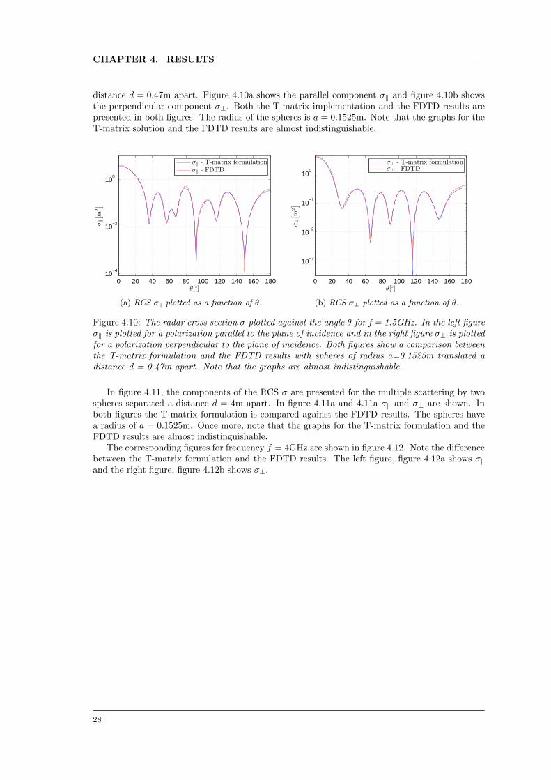
CHAPTER 4. RESULTS

distance d = 0.47m apart. Figure 4.10a shows the parallel component σ‖ and figure 4.10b showsthe perpendicular component σ⊥. Both the T-matrix implementation and the FDTD results arepresented in both figures. The radius of the spheres is a = 0.1525m. Note that the graphs for theT-matrix solution and the FDTD results are almost indistinguishable.

0 20 40 60 80 100 120 140 160 18010

−4

10−2

100

θ[]

σ‖

[

m2]

σ‖ - T-matrix formulationσ‖ - FDTD

(a) RCS σ‖ plotted as a function of θ.

0 20 40 60 80 100 120 140 160 180

10−3

10−2

10−1

100

θ[]σ⊥

[

m2]

σ⊥ - T-matrix formulationσ⊥ - FDTD

(b) RCS σ⊥ plotted as a function of θ.

Figure 4.10: The radar cross section σ plotted against the angle θ for f = 1.5GHz. In the left figureσ‖ is plotted for a polarization parallel to the plane of incidence and in the right figure σ⊥ is plottedfor a polarization perpendicular to the plane of incidence. Both figures show a comparison betweenthe T-matrix formulation and the FDTD results with spheres of radius a=0.1525m translated adistance d = 0.47m apart. Note that the graphs are almost indistinguishable.

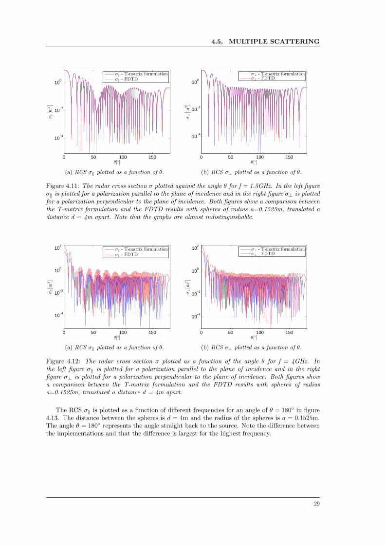
In figure 4.11, the components of the RCS σ are presented for the multiple scattering by twospheres separated a distance d = 4m apart. In figure 4.11a and 4.11a σ‖ and σ⊥ are shown. Inboth figures the T-matrix formulation is compared against the FDTD results. The spheres havea radius of a = 0.1525m. Once more, note that the graphs for the T-matrix formulation and theFDTD results are almost indistinguishable.

The corresponding figures for frequency f = 4GHz are shown in figure 4.12. Note the differencebetween the T-matrix formulation and the FDTD results. The left figure, figure 4.12a shows σ‖and the right figure, figure 4.12b shows σ⊥.

28

4.5. MULTIPLE SCATTERING

0 50 100 150

10−4

10−2

100

θ[]

σ‖

[

m2]

σ‖ - T-matrix formulationσ‖ - FDTD

(a) RCS σ‖ plotted as a function of θ.

0 50 100 150

10−4

10−2

100

θ[]

σ⊥

[

m2]

σ⊥ - T-matrix formulationσ⊥ - FDTD

(b) RCS σ⊥ plotted as a function of θ.

Figure 4.11: The radar cross section σ plotted against the angle θ for f = 1.5GHz. In the left figureσ‖ is plotted for a polarization parallel to the plane of incidence and in the right figure σ⊥ is plottedfor a polarization perpendicular to the plane of incidence. Both figures show a comparison betweenthe T-matrix formulation and the FDTD results with spheres of radius a=0.1525m, translated adistance d = 4m apart. Note that the graphs are almost indistinguishable.

0 50 100 150

10−4

10−2

100

102

θ[]

σ‖

[

m2]

σ‖ - T-matrix formulationσ‖ - FDTD

(a) RCS σ‖ plotted as a function of θ.

0 50 100 150

10−4

10−2

100

102

θ[]

σ⊥

[

m2]

σ⊥ - T-matrix formulationσ⊥ - FDTD

(b) RCS σ⊥ plotted as a function of θ.

Figure 4.12: The radar cross section σ plotted as a function of the angle θ for f = 4GHz. Inthe left figure σ‖ is plotted for a polarization parallel to the plane of incidence and in the rightfigure σ⊥ is plotted for a polarization perpendicular to the plane of incidence. Both figures showa comparison between the T-matrix formulation and the FDTD results with spheres of radiusa=0.1525m, translated a distance d = 4m apart.

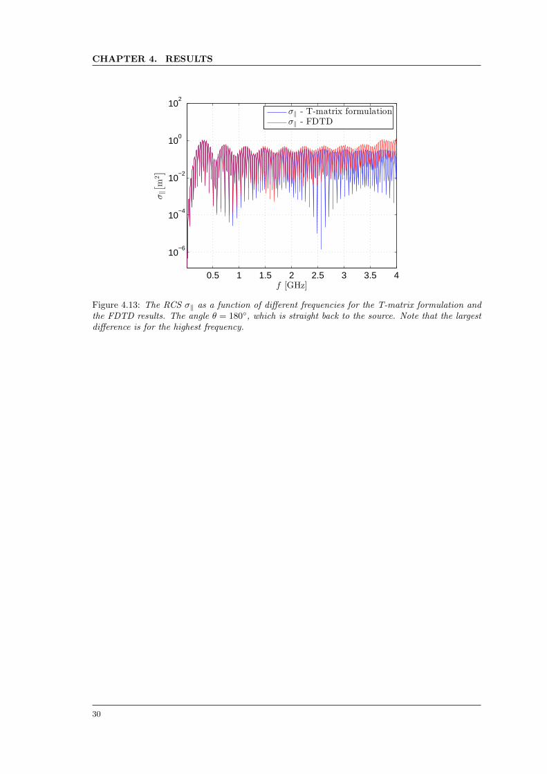
The RCS σ‖ is plotted as a function of different frequencies for an angle of θ = 180 in figure4.13. The distance between the spheres is d = 4m and the radius of the spheres is a = 0.1525m.The angle θ = 180 represents the angle straight back to the source. Note the difference betweenthe implementations and that the difference is largest for the highest frequency.

29

CHAPTER 4. RESULTS

0.5 1 1.5 2 2.5 3 3.5 4

10−6

10−4

10−2

100

102

f [GHz]

σ‖

[

m2]

σ‖ - T-matrix formulationσ‖ - FDTD

Figure 4.13: The RCS σ‖ as a function of different frequencies for the T-matrix formulation andthe FDTD results. The angle θ = 180, which is straight back to the source. Note that the largestdifference is for the highest frequency.

30

Chapter 5

Discussion

In this chapter, the results from chapter 4 will be analysed and discussed in the two followingsections. The first four implementation steps are considered to be validation steps while the mainresults of the project are obtained in the last implementation step. Therefore, the first section willdiscuss the results in section 4.1-4.4 regarding the validation and the second section will discussthe main results from section 4.5. Subsequently follows a section regarding possible expansionsand further studies. As a final conclusion, the aim and goal of the project will be evaluated.

5.1 Analysis of the validation

In the first implementation step the field of an incident plane wave, expressed in spherical vectorwaves, was implemented and as expected they are just lines of constant phase, see figure 4.1. Ifthe criterion for lmax is not fulfilled, the correct solution will not be reached. Instead, the solutionwill look strange at the boundaries of the solution as the distance r from the origin increases.

The results in the second implementation step are satisfying since they show that the imple-mentation well agrees with the highly resolved FDTD results for the near field and exactly withthe Mie reference solution for the far field, see figures 4.2-4.5. Since there are no differences in thegraphs for the far field and small differences in the near field figures, those deviations seem to becaused by the error created by the numerical implementation.

When translating the incident field, the same results are achieved as in the first implementationstep and hence the implementation of the translation matrix R is considered to be correct, seefigure 4.6. The translation matrices R and P are also checked against the translation quantitydefined in equation (2.58).

In the fourth implementation step, the translated sphere was introduced. The results regardingthe translated scattered field showed that the T-matrix implementation for a sphere agreed withthe reference solution, see figures 4.7 and 4.8 . When shifting the sphere further away from theorigin, the early Wigner implementation [21] failed due to large input arguments. This might bedue to the large inputs to the function calculating the factorials. Therefore the recursive Wignerimplementation was performed. This implementation agreed with those presented at [25] and isconsidered correct.

To summarize this section, the results in the first four steps agree with the expectations andthe theory. The validation of these steps makes the results and analysis of the multiple scatteringtrustworthy.

5.2 Analysis of the main results

The first comparison made in section 4.5 was the near field figures with two spheres separated adistance d = 0.47m apart. The T-matrix implementation agrees well with the FDTD results infigure 4.9. One could also see that the scattered fields are affected by the interaction between thespheres. In the figures regarding the RCS, figure 4.10-4.12, one can conclude that the numericalerrors at longer propagation distances increase for higher frequencies.

The numerical dispersion is clearly seen in figure 4.13 where the monostatic RCS is plottedas a function of the frequency. The figure shows that the numerical error is larger for f = 4GHzthan for f = 1.5GHz.

31

CHAPTER 5. DISCUSSION

The numerical dispersion could be smaller if the resolution of the problem would have beenincreased. A higher resolution on the other hand yields a larger computational time. An investi-gation regarding this subject in order to find a better understanding about the relation betweenresolution and computational time is therefore desirable. The implementation of the T-matrixformulation makes is possible to do so.

In the case with two spheres, the implementation of the expansion coefficients fn is madeaccording to equation (2.73). The equation for the expansion coefficients uses the inverse of amatrix. For large distances or for large lmax, the inverse of the matrix could create a singularmatrix and thereby a not trustworthy solution. In these cases it might be more effective toimplement the solution using iterations. Meanwhile an iterative solution is not as exact as thesolution implemented here, it might be useful for some applications.

5.3 Further studies

The simplest suggestion for further studies is to add more than two spheres in the multiple scatter-ing since the only difference is to iteratively calculate the fpn according to equation 2.69. Anotherrelevant continuation of the project would be to implement the T-matrix formulation for a dielec-tric sphere since the only difference is to change the entries in the matrix T . Additionally onecould use other objects, e.g. a disc, or altering the angle of the incident wave. This is possiblehowever the changes increases the complexity since we then lose the simplicity of m = 1.

An interesting expansion would be to further investigate the criterion for lmax for two spheres.It is intuitive to believe that the value of lmax for two spheres would depend on the distancebetween the spheres, which in other words symbolises the whole region of the scattering. As theconvergence test shows, this is not the case. Sufficient information regarding this subject is notfound, which is due to shortage of time. A short note is made in [8] but further investigationwould be interesting.

Finally a comment should be made about the comparison of the T-matrix formulation and theFDTD results. In the report some results regarding this subject is presented mostly in order toprove that the aim is reached. Even though it is not a direct expansion of this thesis it would beinteresting to further investigate the numerical dispersion in the FDTD results with help of theT-matrix formulation.

5.4 Goal completion

Finally we have reached the time when the results will be compared with the aim and goal describedin section 1.2 and 1.3. The goal was to accurately model multiple scattering by two spheres, whereone or both spheres were translated along the z-axis. This goal is considered accomplished since allresults show that the implementation agrees with the reference solution. The comparison with theFDTD-code also shows similar behaviour except for the deviations considered to be the numericaldispersion in the FDTD at higher frequencies.

Regarding the aim, which was to compare the analytical results with those numerical from theFDTD in order to validate the FDTD-code is also considered achieved, even though most of theinteresting parts regarding this investigation remain.

32

Chapter 6

Bibliography

[1] E.F. Knott, J.F. Shaeffer, M.T. Tuley. Radar Cross Section, 2nd ed. Boston : Artech House,1993.

[2] J. Fagerstrom. Berakningsmetoder for radarmalarea. En oversikt. FOA-R-97-00553-615-SE.ISSN 1104-9154. Linkoping, Sweden. August 1997.

[3] A. Taflove. Computational electrodynamics: The Fininte-Difference time-domain method, 3rded. Boston: Artech House, 2005.

[4] T. Martin. Dipsersion compensation for Huygens’ sources and far zone transformation inFDTD in IEEE Trans. on Antennas and Propag., Vol 48, No 4. 2000.

[5] P.C. Waterman. Matrix formulation of Electromagnetic Scattering in Proc. IEEE 53, 805.1965.

[6] P.C. Waterman. Symmetry, Unitarity, and Geometry in Electromagnetic Scattering* in Phys-ical Review D, Vol. 3, No. 4. 1971.

[7] M.I. Mishchenko, N.T. Zakharova, N.G. Khlebtsov, T.Wridet, G.Videen. T-matrix theoryof electromagnetic scattering by particles and its applications: a comprehensive referencedatabase in Journal of quantitative spectroscopy & radiative transfer. Elsevier Ltd, 2004.

[8] G. Peterson, S. Strom. T Matrix for Electromagnetic Scattering from an Arbitrary Numberof Scatterers and Representations of E(3)* in Physical Review D, Vol. 8, No. 10, 1973.

[9] G. Kristensson. Multiple scattering by a collection of randomly located obstacles. Part 1:Theory - coherent fields. Lund university, Tech. Rep. LUTEDX/(TEAT-7235)/1-49/(2014),2014. (Accepted to J. Quant. Spectrosc. Radiat. Transfer)

[10] Y.C. Tzeng, A.K. Fung. T-matrix approach to multiple scattering by EM waves from N-spheresin Journal of electromagnetic waves and applications, Vol.8, No. 1, 1994.

[11] V.K. Varadan, V.V Varadan. Field representations and introduction to scattering. Amster-dam: North-Halland, 1991.

[12] A. Bostrom, G. Kristensson, S. Strom. Transformation properties of plane, spherical andcylindrical scalar and vector wave functions. Amsterdam: Elsevier Science Publisher, 1991 in[11].

[13] G. Kristensson. Spridningsteori med antenntillampningar [Scattering theory with antenna ap-plications]. Lund: Studentlitteratur, 1999.

[14] D.J. Griffiths. Introduction to electrodynamics, 3rd ed. Pearson Education Inc, 2008.

[15] A.R. Edmonds. Angular Momentum in Quantum Mechanics. Princeton University Press,1960.

[16] W.J.Wiscombe. Improved Mie scattering algorithms in Applied optics, Vol. 19, No. 9. 1 May1980

[17] J.E. Hansen. Spherical near-field antenna measurements. London: Peter Peregrinus Ltd, 1988.

33

CHAPTER 6. BIBLIOGRAPHY

[18] J.R. Allardice, E.C. Le Ru. Convergence of Mie theory series: criteria for far-field and near-field properties in Applied Optics. 53, 7224-7229, 2014.

[19] T. Martin. An improved near- to far-zone transformation for the Finite-difference time-domain method in IEEE Trans. on Antennas and Propag., Vol 46, No 9. 1998.

[20] C.W. Trueman, R.J. Luebbers, S.R. Mishra, C. Larose. FDTD computation of the RCS ofhigh permittivity cubes in IEEE Antennas and Propagation Society International Symposium,Vol 2, 1993.

[21] K. Kraus. Mathworks - File exchange. Wigner 3jSymbol - File exchange http:

//www.mathworks.com/matlabcentral/fileexchange/20619-wigner3j-symbol/

content/Wigner3j.m. Online, accessed 2015-03-25.

[22] E.O. Steinborn, E.J. Weninger. Programs for the coupling of spherical harmonics in ComputerPhysics Communications 25, 1982.

[23] R.E. Tuzun, P. Burkhardt, D Secrest. Accurate computation of individual and tables of 3-jand 6-j symbols in Computer Physics Communications 112, 1998.

[24] K. Schulten, R.G. Gordon. Exact recursive evaluation of 3j- and 6j-coefficients for quantum-mechanical coupling of angular momenta in Journal of mathematical physics 16, 1961.

[25] Wolfram Alpha. Wigner 3jSymbol https://www.wolframalpha.com/input/?i=wigner+3j&lk=3. Online, accessed 2015-04-09.

[26] G.T. Ruck, D.E. Barrick, W.D Stuart, C.K Krichbaum. Radar Cross Section Handbook, Vol1. Carlifornia: Penisula Publishing, 2002.

34

Appendix A

Vector spherical harmonics

Vector spherical harmonics are essential in scattering theory. In this appendix we will start withdefining the Legendre polynomials and functions, which are needed in order to define the sphericalharmonics which later can be transformed into vector spherical harmonics [13].

A.1 Legendre polynomials and functions

The Legendre polynomials can be defined in several ways. In this thesis we will define them usingthe so called generating function F (x, t) = (1− 2xt− t2)−1/2 as

1

(1− 2xt− t2)1/2=

∞∑l=0

Pl(x)tl, |t| < 1, (A.1)

where Pl are the Legendre polynomials. With series expansion the series representation of theLegendre polynomials will be

Pl(x) =

[l/2]∑k=0

(−1)k(2l − 2k)!

2lk!(l − k)!(l − 2k)!xl−2k. (A.2)

The associated Legendre functions are for non-negative index m defined as

Pml (x) = (1− x2)m/2dm

dxmPl(x), x ∈ [−1, 1], (A.3)

where Pl are the Legendre polynomials defined earlier. In spherical coordinates the associatedLegendre functions are defined as

Pml (cos θ) = sinm θdm

d(cos θ)mPl(cos θ), θ ∈ [0, π]. (A.4)

A.2 Spherical harmonics

The spherical harmonics Yσml(θ, φ) are defined as

Yσml(θ, φ) =

√εm2π

√2l + 1

2

(l −m)!

(l +m)!Pml (cos θ)

cosmφsinmφ

(A.5)

where the indices σ,m and l are

σ =

eo

, m = 0, 1, 2, . . . , l, l = 0, 1, . . . (A.6)

and the Neumann factor εm is defined to be

εm = 2− δm0 i.e.

ε0 = 1

εm = 2,m > 0. (A.7)

35

APPENDIX A. VECTOR SPHERICAL HARMONICS

This definition of the spherical harmonics only uses non-negative values for the azimuth index m.The value σ = e (even) or σ = o (odd) corresponds to the even or odd trigonometric azimuthfunctions cosmφ respectively sinmφ. With this definition, the spherical harmonics will always bereal in opposite with the definitions using eimφ, with m = −l, . . . ,−1,−0, 1, . . . , l.

The spherical harmonics are often designated as Yσml(r) since the unit vector of the positionvector is r = x sin θ cosφ + y sin θ cosφ + z cos θ, which means that we do not need to use theangels θ and φ in the argument.

A.3 Vector spherical harmonics

A vector field F(r) can be expanded in the earlier defined spherical harmonics as

F(r) =

∞∑l=0

l∑m=0

∑σ=e,o

aσmlYσml(r). (A.8)

The disadvantage with this expansion is that the coefficients aσml are vector-valued. Since it willbe a great advantage to let the coefficients be scalar-valued, we introduce new basis functions withthe vector nature built in. The new basis functions are called vector spherical harmonics and aredefined as

A1σml(r) =1√

l(l + 1)∇× (rYσml(r)) =

1√l(l + 1)

∇Yσml(r)× r

A2σml(r) =1√

l(l + 1)r∇Yσml(r)

A3σml(r) = rYσml(r)

(A.9)

where l = 0, 1, 2, 3, . . . , m = 0, 1, 2, . . . l and σ = e, o. For l = 0, A1σ00(r) and A2σ00(r) are notwell defined since both the nominator and the denominator is zero. To solve this, we define thevector spherical harmonics to be zero in that case, i.e. A1σ00(r) = A2σ00(r) = 0. An alternativeto the earlier defined vector spherical harmonics are expressed using the spherical basis functionsr, θ, φ. The vector spherical harmonics are then

A1σml(r) =1√

l(l + 1)

(θ

1

sin θ

∂

∂φYσml(r)− φ ∂

∂θYσml(r)

)A2σml(r) =

1√l(l + 1)

(θ∂

∂θYσml(r) + φ

1

sin θ

∂

∂φYσml(r)

)A3σml(r) = rYσml(r)

(A.10)

36

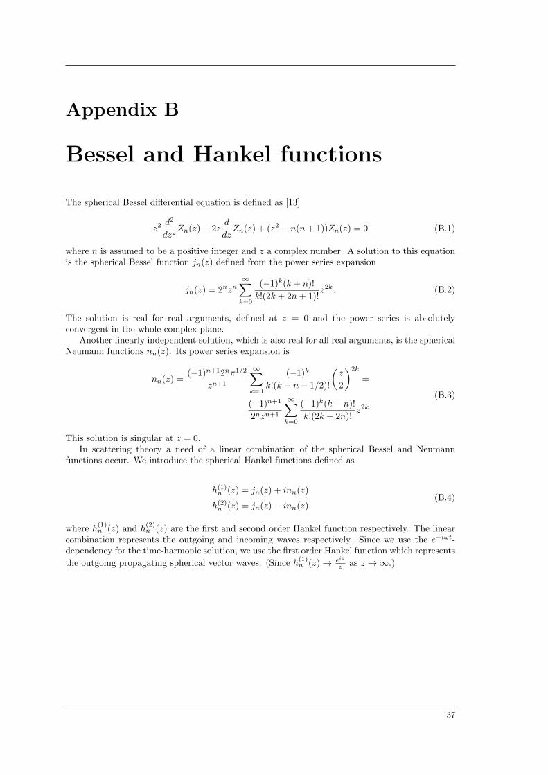
Appendix B

Bessel and Hankel functions

The spherical Bessel differential equation is defined as [13]

z2 d2

dz2Zn(z) + 2z

d

dzZn(z) + (z2 − n(n+ 1))Zn(z) = 0 (B.1)

where n is assumed to be a positive integer and z a complex number. A solution to this equationis the spherical Bessel function jn(z) defined from the power series expansion

jn(z) = 2nzn∞∑k=0

(−1)k(k + n)!

k!(2k + 2n+ 1)!z2k. (B.2)

The solution is real for real arguments, defined at z = 0 and the power series is absolutelyconvergent in the whole complex plane.

Another linearly independent solution, which is also real for all real arguments, is the sphericalNeumann functions nn(z). Its power series expansion is

nn(z) =(−1)n+12nπ1/2

zn+1

∞∑k=0

(−1)k

k!(k − n− 1/2)!

(z

2

)2k

=

(−1)n+1

2nzn+1

∞∑k=0

(−1)k(k − n)!

k!(2k − 2n)!z2k

(B.3)

This solution is singular at z = 0.In scattering theory a need of a linear combination of the spherical Bessel and Neumann

functions occur. We introduce the spherical Hankel functions defined as

h(1)n (z) = jn(z) + inn(z)

h(2)n (z) = jn(z)− inn(z)

(B.4)

where h(1)n (z) and h

(2)n (z) are the first and second order Hankel function respectively. The linear

combination represents the outgoing and incoming waves respectively. Since we use the e−iωt-dependency for the time-harmonic solution, we use the first order Hankel function which represents

the outgoing propagating spherical vector waves. (Since h(1)n (z)→ eiz

z as z →∞.)

37