Rob FowlerRenaissance Computing Institute

Oct 28, 2006

Performance Measurement for LQCD:More New Directions.

GOALS (of This Talk)

• Quick overview of capabilities.– Bread and Butter Tools vs. Research

• Performance Measurement on Leading Edge Systems.

• Plans for SciDAC-2 QCD– Identify useful performance experiments– Deploy to developers

• Install. Write scripts and configuration files.– Identify CS problems

• For RENCI and SciDAC PERI• For our friends – SciDAC Enabling Tech. Ctrs/Insts.

• New proposals and projects.

NSF Track 1 Petascale RFP

• $200M over 5 years for procurement.– Design evaluation, benchmarking, …, buy system.– Separate funding for operations.– Expected funding from science domain

directorates to support applications.

• Extrapolate performance of model apps:– A big DNS hydrodynamics problem.– A lattice-gauge QCD calculation in which 50 gauge

configurations are generated on an 84^3*144 lattice with a lattice spacing of 0.06 fermi, the strange quark mass m_s set to its physical value, and the light quark mass m_l = 0.05*m_s. The target wall-clock time for this calculation is 30 hours.

– A Proteomics/molecular dynamics problem.

The other kind of HPC.

Google’s new data center. Dalles, Oregon

Moore's lawCircuit element count doubles every NN months. (NN ~18)

• Why: Features shrink, semiconductor dies grow.

• Corollaries: Gate delays decrease. Wires are relatively longer.

• In the past the focus has been making "conventional" processors faster.

– Faster clocks– Clever architecture and implementation instruction-level parallelism.– Clever architecture (and massive caches) ease the “memory wall”

problem.• Problems:

– Faster clocks --> more power (P ~ V2F)– More power goes to overhead: cache, predictors, “Tomasulo”, clock, …– Big dies --> fewer dies/wafer, lower yields, higher costs– Together --> Power hog processors on which some signals take 6

cycles to cross.

Competing with charcoal?

Thanks to Bob Colwell

Why is performance not obvious?

Hardware complexity– Keeping up with Moore’s law with one thread.– Instruction-level parallelism.

• Deeply pipelined, out-of-order, superscalar, threads.– Memory-system parallelism

• Parallel processor-cache interface, limited resources.• Need at least k concurrent memory accesses in flight.

Software complexity– Competition/cooperation with other threads– Dependence on (dynamic) libraries.– Compilers

• Aggressive (-O3+) optimization conflicts with manual transformations.

• Incorrectly conservative analysis and optimization.

Processors today

• Processor complexity: – Deeply pipelined, out of order execution.

• 10s of instructions in flight• 100s of instructions in “dependence window”

• Memory complexity: – Deep hierarchy, out of order, parallel.

• Parallelism necessary: 64 bytes/100ns 640 MB/sec.• Chip complexity:

– Multiple cores, – Multi-threading, – Power budget/power state adaptation.

• Single box complexity: – NICs, I/O controllers compete for

processor and memory cycles. – Operating systems and external perturbations.

• Single thread ILP– Instruction pipelining constraints, etc.– Memory operation scheduling for latency, BW.

• Multi-threading CLP– Resource contention within a core

• Memory hierarchy• Functional units, …

• Multi-core CLP– Chip-wide resource contention

• Shared on-chip components of the memory system• Shared chip-edge interfaces

Today’s issues.It’s all about contention.

Challenge: Tools will need to attribute contentioncosts to all contributingprogram/hardware elements.

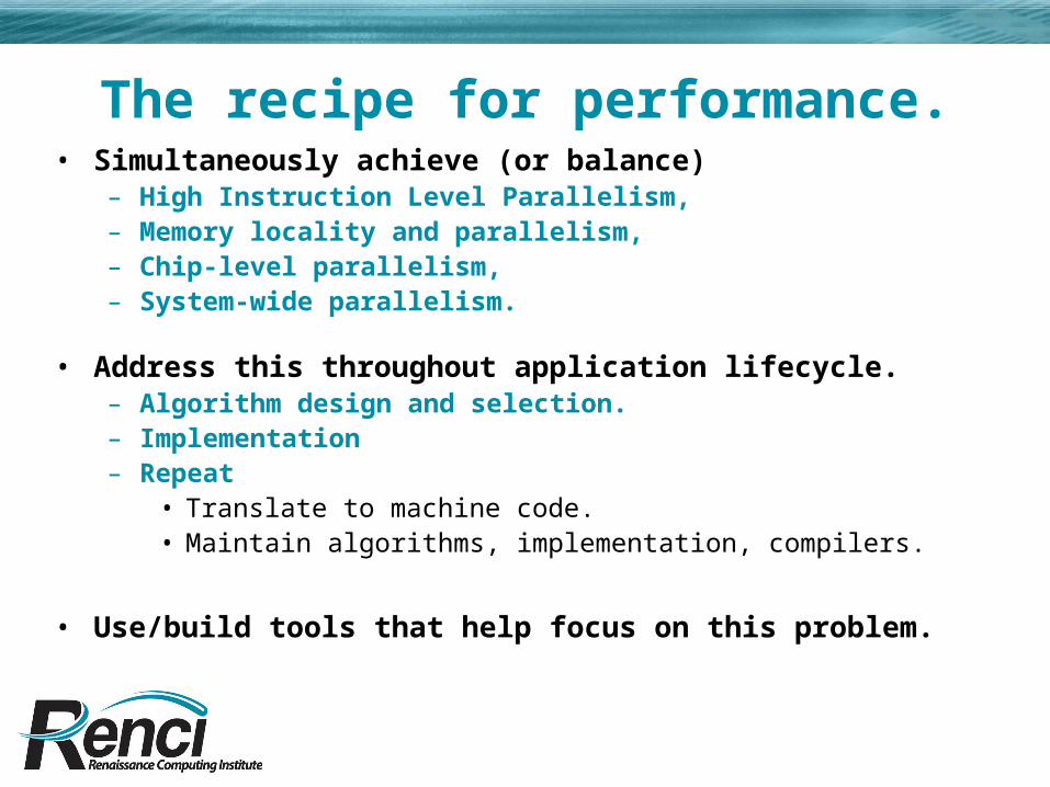
The recipe for performance.• Simultaneously achieve (or balance)

– High Instruction Level Parallelism, – Memory locality and parallelism, – Chip-level parallelism,– System-wide parallelism.

• Address this throughout application lifecycle.

– Algorithm design and selection.– Implementation– Repeat

• Translate to machine code.• Maintain algorithms, implementation, compilers.

• Use/build tools that help focus on this problem.

Performance Tuning in Practice

One proposednew tool GUI

It gets worse: Scalable HECAll the problems of on-node efficiency, plus• Scalable parallel algorithm design.• Load balance,• Communication performance,• Competition of communication with

applications,• External perturbations,• Reliability issues:

– Recoverable errors performance perturbation.– Non-recoverable error You need a plan B

• Checkpoint/restart (expensive, poorly scaled I/O)• Robust applications

All you need to know about software engineering.

'The Hitchiker's Guide to the Galaxy, in a moment of reasoned lucidity which is almost unique among its current tally of five million, nine hundred and seventy-three thousand, five hundred and nine pages, says of the Sirius Cybernetics Corporation products that “it is very easy to be blinded to the essential uselessness of them by the sense of achievement you get from getting them to work at all. In other words - and this is the rock-solid principle on which the whole of the Corporation's galaxywide success is founded -- their fundamental design flaws are completely hidden by their superficial design flaws.”

(Douglas Adams, "So Long, and Thanks for all the Fish")

A Trend in Software Tools

Featuritis in extremis?

What must a useful tool do?• Support large, multi-lingual (mostly compiled)

applications– a mix of of Fortran, C, C++ with multiple compilers

for each– driver harness written in a scripting language– external libraries, with or without available source– thousands of procedures, hundreds of thousands of

lines

• Avoid– manual instrumentation– significantly altering the build process– frequent recompilation

• Multi-platform, with ability to do cross-platform analysis

Tool Requirements, II• Scalable data collection and analysis• Work on both serial and parallel

codes • Present data and analysis effectively

– Perform analyses that encourage models and intuition, i.e., data knowledge.

– Support non-specialists, e.g., physicists and engineers.

– Detail enough to meet the needs of computer scientists.

– (Can’t be all things to all people)

Example: HPCToolkit

GOAL: On-node measurement to support tuning, mostly by compiler writers.

• Data collection– Agnostic -- use any source that collects

“samples” or “profiles”– Use hardware performance counters in EBS

mode. Prefer in “node-wide” measurement.– Unmodified, aggressively-optimized target

code• No instrumentation in source or object

– Command line tools designed to be used in scripts.• Embed performance tools in the build process.

HPCToolkit, II• Compiler-neutral attribution of costs

– Use debugging symbols + binary analysis to characterize program structure.

– Aggregate metrics by hierarchical program structure• ILP Costs depend on all the instructions in

flight.• (Precise attribution can be useful, but isn’t

always necessary, possible, or economic.)– Walk the stack to characterize dynamic

context• Asynchronous stack walk on optimized code is

“tricky”– (Emerging Issue: “Simultaneous

attribution” for contention events)

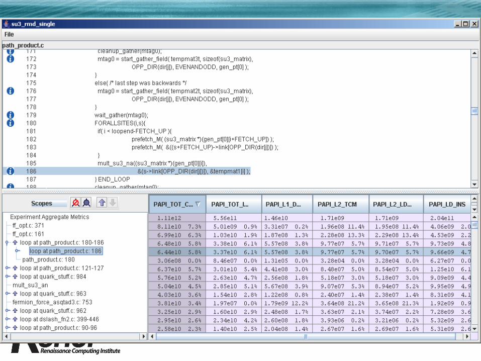
HPCToolkit, III• Data Presentation and Analysis

– Compute derived metrics.• Examples: CPI, miss rates, bus utilization, loads per

FLOP, cycles – FLOP, …• Search and sort on derived quantities.

– Encourage (enforce) top-down viewing and diagnosis.

– Encode all data in “lean” XML for use by downstream tools.

Data Collection RevisitedMust analyze unmodified, optimized binaries!

• Inserting code to start, stop and read counters has many drawbacks, so don’t do it! (At least not for our purposes.)– Expensive, both at both instrumentation and run times– Nested measurement calipers skew results– Instrumentation points must inhibit optimization and ILP

fine grain results are nonsense.• Use hardware performance monitoring (EBS) to collect

statistical profiles of events of interest.• Exploit unique capabilities of each platform.

– event-based counters: MIPS, IA64, AMD64, IA32, (Power)– ProfileMe instruction tracing: Alpha

• Different architectural designs and capabilities require “semantic agility”.

• Instrumentation to quantify on-chip parallelism is lagging.See “FHPM Workshop” at Micro-39.

• Challenge: Minimizing jitter large-scale.

Management Issue: EBS on Petascale Systems

• Hardware on BG/L and XT3 both support event based sampling.

• Current OS kernels from vendors do not have EBS drivers.

• This needs to be fixed!– Linux/Zeptos? Plan 9?

• Issue: Does event-based sampling introduce “jitter”?– Much less impact than using fine-grain calipers.– Not unless you have much worse performance

problems.

In-house customers needed for success!

At Rice, we (HPC compiler group) were our own customers.

RENCI projects as customers.– Cyberinfrastructure Evaluation Center– Weather and Ocean

• Linked Environments for Atmospheric Discovery• SCOOPS (Ocean and shore)• Disaster planning and response

– Lattice Quantum Chromodynamics Consortium– Virtual Grid Application Development Software – Bioportal applications and workflows.

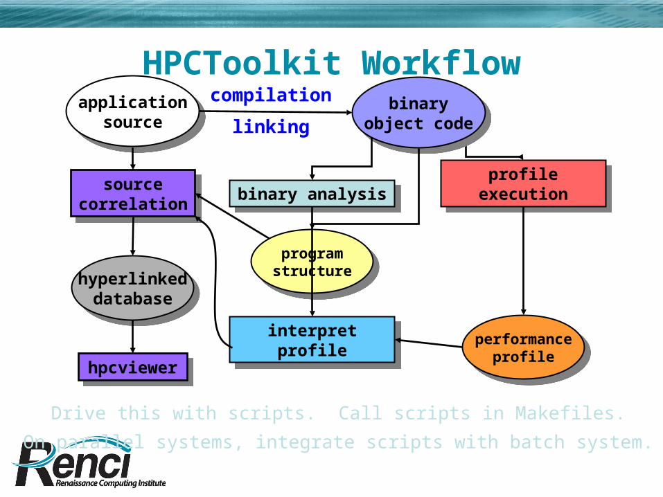
HPCToolkit Workflowapplication

source

applicationsource

profile execution

profile execution

performanceprofile

performanceprofile

binaryobject code

binaryobject code

compilation

linking

binary analysisbinary analysis

programstructure

programstructure

interpret profileinterpret profile

source correlation

source correlation

hyperlinkeddatabase

hyperlinkeddatabase

hpcviewer

hpcviewer

Drive this with scripts. Call scripts in Makefiles.

On parallel systems, integrate scripts with batch system.

CSPROF• Extend HPCToolkit to use statistical sampling

to collect dynamic calling contexts. – Which call path to memcpy or MPI_recv was

expensive?• Goals

– Low, controllable overhead and distortion.– Distinguish costs by calling context,

where context = full path.– No changes to the build process.– Accurate at the highest level of optimization.– Work with binary-only libraries, too.– Distinguish “busy paths” from “hot leaves”

• Key ideas– Run unmodified, optimized binaries.

• Very little overhead when not actually recording a sample.

– Record samples efficiently

Efficient CS Profiling: How to. • Statistical sampling of performance counters.

– Pay only when sample taken.– Control overhead %, total cost by changing rate.

• Walk the stack from asynchronous events.– Optimized code requires extensive, correct compiler

support. – (Or we need to identify epilogues, etc by analyzing

binaries.)• Limit excessive stack walking on repeated

events.– Insert a high-water mark to identify “seen before”

frames.• We use a “trampoline frame”. Other implementations

possible.– Pointers from frames in “seen before” prefix to

internal nodes of CCT to reduce memory touches.

CINT2000 benchmarks

BenchmarkBase time (seconds)

gprof overhead

(%)

gprof number of calls

csprof overhead

(%)

csprof data file size (bytes)

164.gzip 479 53 1.960E+09 4.2 270,194175.vpr 399 53 1.558E+09 2 98,678176.gcc 250 78 9.751E+08 N/A N/A181.mcf 475 19 8.455E+08 8 30,563186.crafty 196 141 1.908E+09 5.1 12,534,317197.parser 700 167 7.009E+09 4.6 12,083,741252.eon 263 263 1.927E+09 3.4 757,943253.perlbmk 473 165 2.546E+09 2.5 1,757,749254.gap 369 39 9.980E+08 4.1 2,215,955255.vortex 423 230 6.707E+09 5.4 6,060,039256.bzip2 373 112 3.205E+09 1.1 180,790300.twolf 568 59 2.098E+09 3 122,898

Accuracy comparison• Base information collected using DCPI• Two evaluation criteria

– Distortion of relative costs of functions– Dilation of individual functions

• Formulae for evaluation– Distribution

– Time

pctprof ( f ) pctbase( f )f functions( p )

timeprof ( f ) timebase( f )f functions( p )

totaltime(p)

CINT2000 accuracy

Benchmark csprof dist gprof dist csprof time gprof time164.gzip 1.275 6.897 2.043 51.998175,vpr 2.672 7.554 4.32 52.193181.mcf 53.536 29.943 14.152 18.668186.crafty 1.095 14.53 5.002 132.145197.parser 6.871 15.383 3.576 162.547252.eon 1.664 119.063 4.827 242.798253.perlbmk 5.229 8.962 3.025 161.621254.gap 9.307 7.829 4.077 38.038255.vortex 2.895 15.415 3.722 221.453256.bzip2 7.839 16.477 3.699 109.625300.twolf 0.827 6.923 3.05 56.856

Numbers are percentages.

CFP2000 benchmarks

BenchmarkBase time (seconds)

gprof overhead

(%)

gprof number of calls

csprof overhead

(%)

csprof data file size (bytes)

168.wupwise 351 85 2.233E+09 2.5 559,178171.swim 298 0.17 2.401E+03 2 93,729172.mgrid 502 0.12 5.918E+04 2 170,034173.applu 331 0.21 2.192E+05 1.9 317,650177.mesa 272 67 1.658E+09 3 56,676178.galgel 251 5.5 1.490E+07 3.2 756,155179.art 196 2.1 1.110E+07 1.5 76,804183.equake 583 0.75 1.047E+09 7 44,889187.facerec 262 9.4 2.555E+08 1.5 197,114188.ammp 551 2.8 1.006E+08 2.7 93,166189.lucas 304 0.3 1.950E+02 1.9 113,928191.fma3d 428 18 5.280E+08 2.3 232,958200.sixtrack 472 0.99 1.030E+07 1.7 184,030301.apsi 589 12 2.375E+08 1.6 1,209,095

Problem: Profiling Parallel Programs• Sampled profiles can be collected for about 1%

overhead.• How can one productively use this data on large

parallel systems?– Understand the performance characteristics of the

application.• Identify and diagnose performance problems.• Collect data to calibrate and validate performance models.

– Study node-to-node variation.• Model and understand systematic variation.

– Characterize intrinsic, systemic effects in app.• Identify anomalies: app. bugs, system effects.

– Automate everything.• Do little “glorified manual labor” in front of a GUI.• Find/diagnose unexpected problems, not just the expected

ones.• Avoid the “10,000 windows” problem.• Issue: Do asynchronous samples introduce “jitter”?

Statistical Analysis: Bi-clustering• Data Input: an M by P dense matrix of (non-negative)

values.– P columns, one for each process(or).– M rows, one for each measure at each source construct.

• Problem: Identify bi-clusters.– Identify a group of processors that are different from the

others because they are “different” w.r.t. some set of metrics. Identify the set of metrics.

– Identify multiple bi-clusters until satisfied.• The “Cancer Gene Expression Problem”

– The columns represent patients/subjects• Some are controls, others have different, but related cancers.

– The rows represent data from DNA micro-array chips.– Which (groups of) genes correlate (+ or -) with which

diseases?– There’s a lot of published work on this problem.– So, use the bio-statisticians’ code as our starting point.

• E.g., “Gene shaving” algorithm by M.D. Anderson and Rice researchers.

Cluster 1: 62% of variance in Sweep3D

Weight Clone ID -6.39088 sweep.f,sweep:260 -7.43749 sweep.f,sweep:432-7.88323 sweep.f,sweep:435 -7.97361 sweep.f,sweep:438 -8.03567 sweep.f,sweep:437 -8.46543 sweep.f,sweep:543 -10.08360 sweep.f,sweep:538 -10.11630 sweep.f,sweep:242-12.53010 sweep.f,sweep:536 -13.15990 sweep.f,sweep:243 -15.10340 sweep.f,sweep:537 -17.26090 sweep.f,sweep:535

if (ew_snd .ne. 0) then call snd_real(ew_snd, phiib, nib, ew_tag, info)c nmess = nmess + 1c mess = mess + nib else if (i2.lt.0 .and. ibc.ne.0) then leak = 0.0 do mi = 1, mmi m = mi + mio do lk = 1, nk k = k0 + sign(lk-1,k2) do j = 1, jt phiibc(j,k,m,k3,j3) = phiib(j,lk,mi) leak = leak & + wmu(m)*phiib(j,lk,mi)*dj(j)*dk(k) end do end do end do leakage(1+i3) = leakage(1+i3) + leak else leak = 0.0 do mi = 1, mmi m = mi + mio do lk = 1, nk k = k0 + sign(lk-1,k2) do j = 1, jt leak =leak+ wmu(m)*phiib(j,lk,mi)*dj(j)*dk(k) end do end do end do leakage(1+i3) = leakage(1+i3) + leak endif endif

if (ew_rcv .ne. 0) then call rcv_real(ew_rcv, phiib, nib, ew_tag, info) else if (i2.lt.0 .or. ibc.eq.0) then do mi = 1, mmi do lk = 1, nk do j = 1, jt phiib(j,lk,mi) = 0.0d+0 end do end do end do

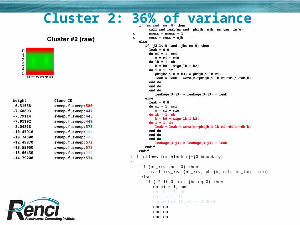
Cluster 2: 36% of variance

Weight Clone ID -6.31558 sweep.f,sweep:580 -7.68893 sweep.f,sweep:447 -7.79114 sweep.f,sweep:445 -7.91192 sweep.f,sweep:449 -8.04818 sweep.f,sweep:573 -10.45910 sweep.f,sweep:284 -10.74500 sweep.f,sweep:285 -12.49870 sweep.f,sweep:572 -13.55950 sweep.f,sweep:575 -13.66430 sweep.f,sweep:286 -14.79200 sweep.f,sweep:574

if (ns_snd .ne. 0) then call snd_real(ns_snd, phijb, njb, ns_tag, info)c nmess = nmess + 1c mess = mess + njb else if (j2.lt.0 .and. jbc.ne.0) then leak = 0.0 do mi = 1, mmi m = mi + mio do lk = 1, nk k = k0 + sign(lk-1,k2) do i = 1, it phijbc(i,k,m,k3) = phijb(i,lk,mi) leak = leak + weta(m)*phijb(i,lk,mi)*di(i)*dk(k) end do end do end do leakage(3+j3) = leakage(3+j3) + leak else leak = 0.0 do mi = 1, mmi m = mi + mio do lk = 1, nk k = k0 + sign(lk-1,k2) do i = 1, it leak = leak + weta(m)*phijb(i,lk,mi)*di(i)*dk(k) end do end do end do leakage(3+j3) = leakage(3+j3) + leak endif endif

c J-inflows for block (j=j0 boundary)c if (ns_rcv .ne. 0) then call rcv_real(ns_rcv, phijb, njb, ns_tag, info) else if (j2.lt.0 .or. jbc.eq.0) then do mi = 1, mmi do lk = 1, nk do i = 1, it phijb(i,lk,mi) = 0.0d+0 end do end do end do

Which performance experiments?

• On-node performance in important operating conditions.– Conditions seen in realistic parallel run.– Memory latency hiding, bandwidth– Pipeline utilization– Compiler and architecture effectiveness.– Optimization strategy issues.

• Where’s the headroom?• Granularity of optimization, e.g., leaf operation vs

wider loops.• Parallel performance measurements

– Scalability through differential call-stack profiling• Performance tuning and regression testing

suite? (Differential profiling extensions.)_

Other CS contributions?

• Computation reordering for performance (by hand or compiler)– Space filling curves or Morton ordering?

• Improve temporal locality.• Convenient rebalancing (non issue for

LQCD?)– Time-skewing?– Loop reordering, …

• Communication scheduling for overlap?