risposta di neuroni singoli sottoposti a stimoli stocastici · risposta di neuroni singoli...
TRANSCRIPT
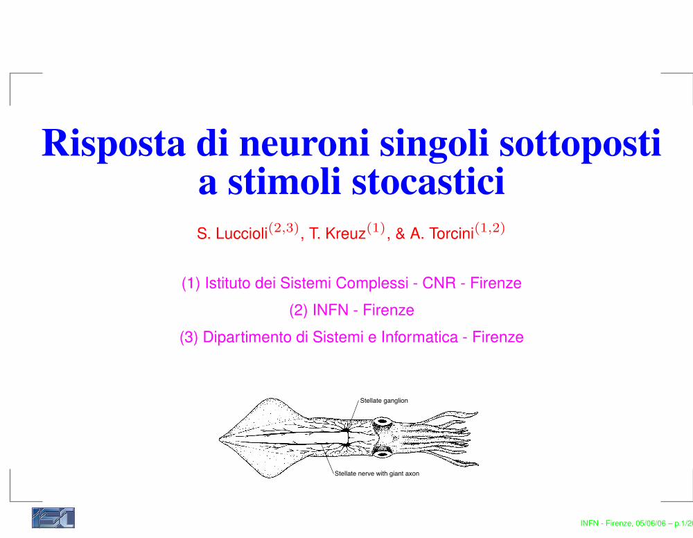
Risposta di neuroni singoli sottopostia stimoli stocasticiS. Luccioli(2,3), T. Kreuz(1), & A. Torcini(1,2)
(1) Istituto dei Sistemi Complessi - CNR - Firenze(2) INFN - Firenze
(3) Dipartimento di Sistemi e Informatica - Firenze
88 Guevara
Stellate nerve with giant axon
Stellate ganglion
Figure 4.1. Anatomical location of the giant axon of the squid. Drawing by TomInoue.
4.2.2 Measurement of the Transmembrane Potential
The large diameter of the axon (as large as 1000 µm) makes it possible toinsert an axial electrode directly into the axon (Figure 4.2A). By placinganother electrode in the fluid in the bath outside of the axon (Figure 4.2B),the voltage difference across the axonal membrane (the transmembranepotential or transmembrane voltage) can be measured. One can alsostimulate the axon to fire by injecting a current pulse with another set ofextracellular electrodes (Figure 4.2B), producing an action potential thatwill propagate down the axon. This action potential can then be recordedwith the intracellular electrode (Figure 4.2C). Note the afterhyperpolar-ization following the action potential. One can even roll the cytoplasm outof the axon, cannulate the axon, and replace the cytoplasm with fluid ofa known composition (Figure 4.3). When the fluid has an ionic composi-tion close enough to that of the cytoplasm, the action potential resemblesthat recorded in the intact axon (Figure 4.2D). The cannulated, internallyperfused axon is the basic preparation that allowed electrophysiologists tosort out the ionic basis of the action potential fifty years ago.
The advantage of the large size of the invertebrate axon is appreciatedwhen one contrasts it with a mammalian neuron from the central nervoussystem (Figure 4.4). These neurons have axons that are very small; indeed,the soma of the neuron in Figure 4.4, which is much larger than the axon,is only on the order of 10 µm in diameter.
4.3 Basic Electrophysiology
4.3.1 Ionic Basis of the Action Potential
Figure 4.5 shows an action potential in the Hodgkin–Huxley model of thesquid axon. This is a four-dimensional system of ordinary differential equa-
INFN - Firenze, 05/06/06 – p.1/20
Collaborazioni in T061 a Firenze
Le linee di ricerca riconducibili a neuroscienze computazionali attualmente attive sono:Dinamica di reti neuronali, effetti del disordine e del ritardo
dr. Rüdiger Zillmer (Borsista – INFN)prof. Roberto Livi (Dip. Fisica – INFN)dr. Antonio Politi (Dir. Ricerca - ISC – CNR)
Risposta di modelli di neurone sottoposti a stimoli stocasticidr. Thomas Kreuz (European Marie-Curie Fellow - ISC – CNR)Stefano Luccioli (Dottorando in Sistemi Complessi – INFN)
Tali studi sono principalmente computazionali, ma si avvalgono di concetti e metodologieproprie della meccanica statistica, della dinamica non-lineare, della teoria dell’informazione.
http://www.fi.isc.cnr.it/users/alessandro.torcini/neurores.html
INFN - Firenze, 05/06/06 – p.2/20

Summary
Introduction to the Hodgkin-Huxley modelCharacterization of the stochastic stimulation protocolAnalysis of the neuronal responses for different noise levelsLooking for coherence in the neuronal responseInfluence of correlations on the coherent responseConclusions
INFN - Firenze, 05/06/06 – p.3/20
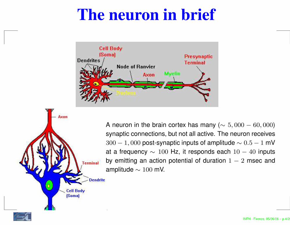
The neuron in brief
A neuron in the brain cortex has many (∼ 5, 000 − 60, 000)synaptic connections, but not all active. The neuron receives300 − 1, 000 post-synaptic inputs of amplitude ∼ 0.5 − 1 mVat a frequency ∼ 100 Hz, it responds each 10 − 40 inputsby emitting an action potential of duration 1 − 2 msec andamplitude ∼ 100 mV.
INFN - Firenze, 05/06/06 – p.4/20
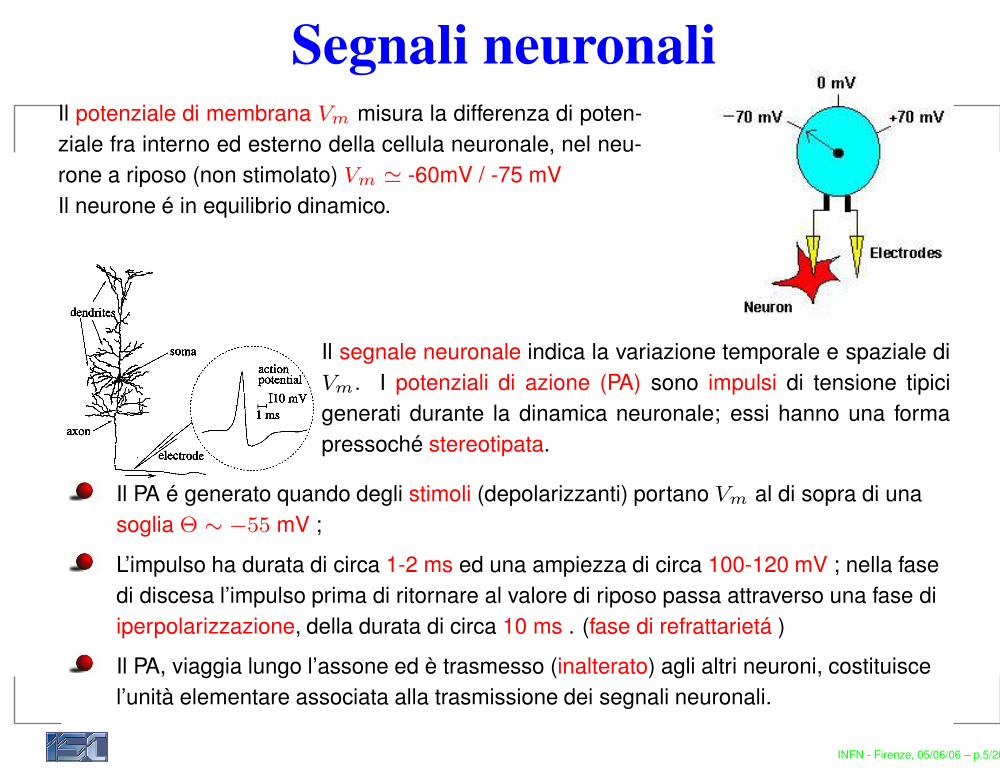
Segnali neuronaliIl potenziale di membrana Vm misura la differenza di poten-ziale fra interno ed esterno della cellula neuronale, nel neu-rone a riposo (non stimolato) Vm ' -60mV / -75 mVIl neurone é in equilibrio dinamico.
Il segnale neuronale indica la variazione temporale e spaziale diVm. I potenziali di azione (PA) sono impulsi di tensione tipicigenerati durante la dinamica neuronale; essi hanno una formapressoché stereotipata.
Il PA é generato quando degli stimoli (depolarizzanti) portano Vm al di sopra di unasoglia Θ ∼ −55 mV ;L’impulso ha durata di circa 1-2 ms ed una ampiezza di circa 100-120 mV ; nella fasedi discesa l’impulso prima di ritornare al valore di riposo passa attraverso una fase diiperpolarizzazione, della durata di circa 10 ms . (fase di refrattarietá )Il PA, viaggia lungo l’assone ed è trasmesso (inalterato) agli altri neuroni, costituiscel’unità elementare associata alla trasmissione dei segnali neuronali.
INFN - Firenze, 05/06/06 – p.5/20
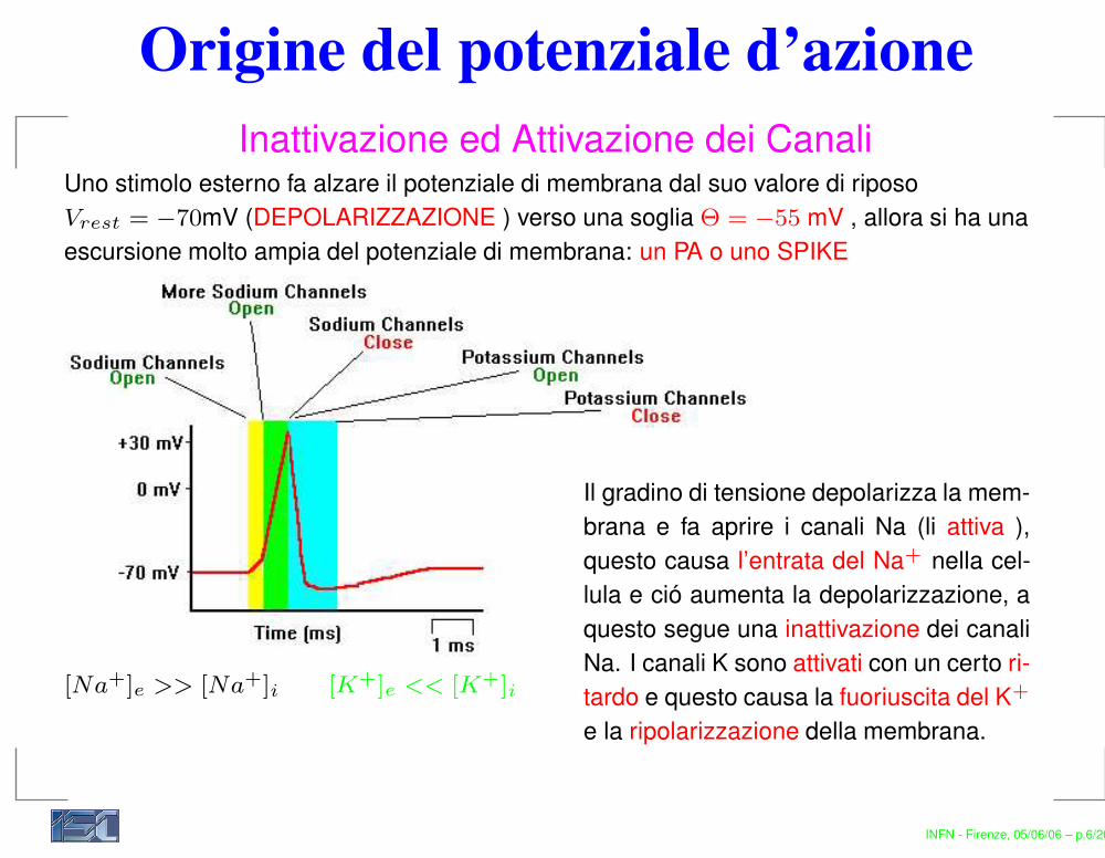
Origine del potenziale d’azioneInattivazione ed Attivazione dei Canali
Uno stimolo esterno fa alzare il potenziale di membrana dal suo valore di riposoVrest = −70mV (DEPOLARIZZAZIONE ) verso una soglia Θ = −55 mV , allora si ha unaescursione molto ampia del potenziale di membrana: un PA o uno SPIKE
[Na+]e >> [Na+]i [K+]e << [K+]i
Il gradino di tensione depolarizza la mem-brana e fa aprire i canali Na (li attiva ),questo causa l’entrata del Na+ nella cel-lula e ció aumenta la depolarizzazione, aquesto segue una inattivazione dei canaliNa. I canali K sono attivati con un certo ri-tardo e questo causa la fuoriuscita del K+
e la ripolarizzazione della membrana.
INFN - Firenze, 05/06/06 – p.6/20

Origine del potenziale d’azioneDepolarizzazione e ripolarizzazione della membrana
Depolarizzazione della membrana
Na+ entra nella cellulaVm → ENa+ = +55 mV
Ripolarizzazione della membrana
K+ lascia la cellulaVm → EK+ = −75 mV
INFN - Firenze, 05/06/06 – p.6/20
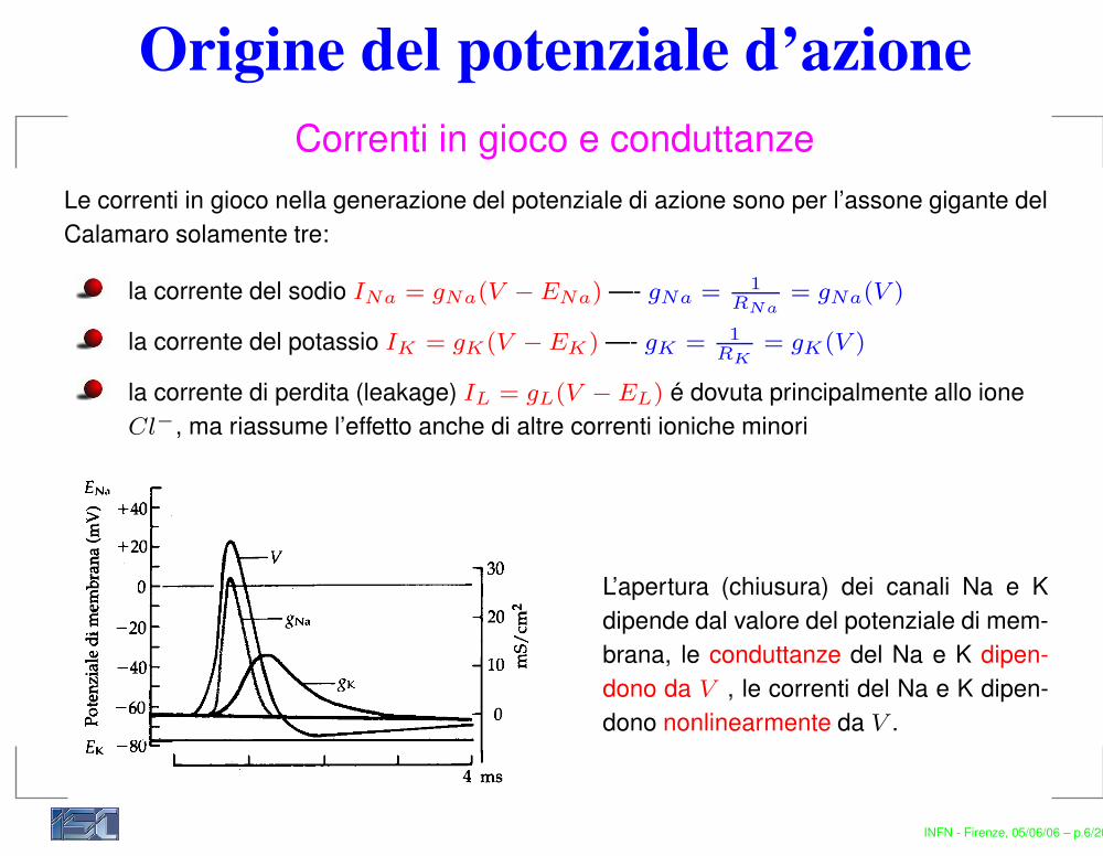
Origine del potenziale d’azioneCorrenti in gioco e conduttanze
Le correnti in gioco nella generazione del potenziale di azione sono per l’assone gigante delCalamaro solamente tre:
la corrente del sodio INa = gNa(V − ENa) —- gNa = 1RNa
= gNa(V )
la corrente del potassio IK = gK(V − EK) —- gK = 1RK
= gK(V )
la corrente di perdita (leakage) IL = gL(V − EL) é dovuta principalmente allo ioneCl−, ma riassume l’effetto anche di altre correnti ioniche minori
L’apertura (chiusura) dei canali Na e Kdipende dal valore del potenziale di mem-brana, le conduttanze del Na e K dipen-dono da V , le correnti del Na e K dipen-dono nonlinearmente da V .
INFN - Firenze, 05/06/06 – p.6/20

Origine del potenziale d’azioneSchema circuitale della membrana
Schema per un pezzetto dimembranaLegge dei NodiI(t) = IC + INa + IK + IL
corrente capacitivaIC = dQ/dt = CdV/dt
correnti ioniche INa e IK
(nonlineari )corrente di perdita (lineare)
CdV
dt= −INa − IK − IL + Isyn(t)
Il problema é calcolare sperimentalmente come variano le conduttanze gNa e gK al variaredel potenziale di membrana, la loro dinamica.
INFN - Firenze, 05/06/06 – p.6/20
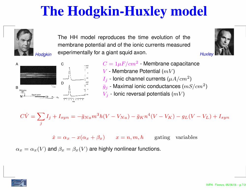
The Hodgkin-Huxley modelThe HH model reproduces the time evolution of themembrane potential and of the ionic currents measuredexperimentally for a giant squid axon.Hodgkin Huxley
4. Dynamics of Excitable Cells 89
A C
B
mV+50
0
-50
mV+50
0
-50
6 7 853 4
ms20 1
D1 mm
Stimulus
Squid axon
EM
Figure 4.2. (A) Giant axon of the squid with internal electrode. Panel A fromHodgkin and Keynes (1956). (B) Axon with intracellularly placed electrode,ground electrode, and pair of stimulus electrodes. Panel B from Hille (2001).(C) Action potential recorded from intact axon. Panel C from Baker, Hodgkin,and Shaw (1961). (D) Action potential recorded from perfused axon. Panel Dfrom Baker, Hodgkin, and Shaw (1961).
Rubber-coveredroller
Axoplasm
Rubber pad
Figure 4.3. Cannulated, perfused giant axon of the squid. From Nicholls, Martin,Wallace, and Fuchs (2001).
tions that describes the three main currents underlying the action potentialin the squid axon. Figure 4.5 also shows the time course of the conductanceof the two major currents during the action potential. The fast inwardsodium current (INa) is the current responsible for generating the upstrokeof the action potential, while the potassium current (IK) repolarizes themembrane. The leakage current (IL), which is not shown in Figure 4.5, ismuch smaller than the two other currents. One should be aware that otherneurons can have many more currents than the three used in the classicHodgkin–Huxley description.
4.3.2 Single-Channel Recording
The two major currents mentioned above (INa and IK) are currents thatpass across the cellular membrane through two different types of channels
C = 1µF/cm2 - Membrane capacitanceV - Membrane Potential (mV )Ij - Ionic channel currents (µA/cm2)gj - Maximal ionic conductances (mS/cm2)Vj - Ionic reversal potentials (mV )
CV =X
j
Ij + Isyn = −gNam3h(V − VNa) − gKn4(V − VK) − gL(V − VL) + Isyn
x = αx − x(αx + βx) x = n, m, h gating variables
αx = αx(V ) and βx = βx(V ) are highly nonlinear functions.
INFN - Firenze, 05/06/06 – p.7/20

The Hodgkin-Huxley modelThe HH model reproduces the time evolution of themembrane potential and of the ionic currents measuredexperimentally for a giant squid axon.Hodgkin Huxley
Constant Current Synaptic Input Isyn = Idc
and VNa , VK , Vl are the corresponding reversal potentials;m` , h` , n` and tm , th , tn represent the saturation valuesand the relaxation times of the gating variables. Detailedvalues of parameters can be found in @11–13#. In this studywe take the external stimulus to be time independent dc cur-rent Iext(t)5Idc which serves as a bifurcation parameter ofthe system.
The synaptic current represents the sum of the currentinputs from all synapses connected to the other neurons. Thissynaptic current is found to be noisy @14#, which we modelas an additive noise from an Ornstein-Uhlenbeck process:
tddIsyn
dt 52Isyn1A2Dj~ t !, ~3!
where j(t) is Gaussian white noise, and D and td are theintensity and the correlation time of the synaptic noise, re-spectively. In numerical simulations we take td52 msec.Numerical integration of Eq. ~1! has been done using thefourth order Runge-Kutta method and the exponentially cor-related synaptic noise in Eq. ~3! using the method of Foxet al. @15# with the integration time step Dt50.02 msec.
Let us consider first the bifurcations in the system ~1! inthe absence of noise (D50). The bifurcation diagram for themembrane potential V as a function of Idc is shown in Fig. 1@16–19#. The birth of limit cycles occurs at Idc5Ic'6.2 mA/cm2 due to the saddle-node bifurcation of peri-odic orbits. The unstable part of the periodic orbits dies atIdc5Ih'9.8 mA/cm2 through the inverse Hopf bifurcation.Thus in the parameter region Idc,Ic the fixed point is theglobal attractor of the system, while for Ic,Idc,Ih the sys-tem possesses two coexisting stable attractors, the fixed pointand the limit cycle. The dependence of the firing rate as afunction of Idc is shown in the inset of Fig. 1.
The focus of interest is the parameter region near the on-set of the saddle-node bifurcation of periodic orbits. In ournumerical experiments, we use three subthreshold values ofdc currents of Idc55.0, 5.5, and 6.0 mA/cm2. With noisetaken into account, the system either fluctuates around thefixed point or makes an excursion into the region of the limitcycle, inducing the trains of periodic oscillations of themembrane potentials. The time series of the membrane po-tential V for four different values of noise intensity for Idc56.0 mA/cm2 are shown in Fig. 2. For small noise inten-sity @Fig. 2~a!# the system spends most of its time fluctuatingaround the rest potential V rest5265 mV, and displays trainsof a few short periodic oscillations, characteristic of the so-called ‘‘rigid excitation.’’ This rigid excitation appears whenthe system in the subthreshold regime spends more time inthe narrow corridorlike neighborhood of the remnants of thelimit cycles due to the tangential nature of the saddle-nodebifurcation of limit cycles @20#. The noise-controlled time
FIG. 1. Bifurcation diagram of a Hodgkin-Huxley neuron underdc current. Here Idc is the bifurcation parameter and V is the mem-brane potential of the limit states. A solid line represents the stablefixed point, filled and unfilled circles represent membrane potentialsof stable and unstable limit cycles, respectively. Inset: The fre-quency f of the stable limit cycle for the Hodgkin-Huxley neuron asa function of Idc . The dotted line is for increasing Idc and the solidline for decreasing Idc .
FIG. 2. Time series of the membrane potentialV for Idc56 mA/cm2 for various noise intensity:~a! D51, ~b! D55, ~c! D510, and ~d! D520.
57 3293COHERENCE RESONANCE IN A HODGKIN-HUXLEY NEURON
4 6 8 10 12Idc (µA/cm2)
0
10
20
30
40
50
60
70
f (H
z)
0 25 50 75 100
time (ms)
-80
-40
0
40
V (m
V)
IHB
ISN
INFN - Firenze, 05/06/06 – p.7/20
Main motivationsA neuron in the brain cortex is subject to a continuous synaptic bombardament ofinputs, resembling a background noise(A. Destexhe, M. Rudolph, D. Paré - Nature Reviews - Neuroscience - 2003)Inputs are mainly originating from the cortex itself, their statistical properties of can be(roughly) summarized as
Frequency range 100 − 200 Hz;Amplitude ∼ 0.5 − 1 mV;Distribution of the arrival times : approximately Poissonian (exponential).
(M.N. Shadlen & W.T. Newsome, J. Neuroscience - 1998)Neurons in the cortex, due to the high connectivity, can receive inputs from the sameaxon: correlation via common drive;
Correlations in the inputs can influence the firing rate of the neuron;Correlations can regulate the flow of neural information: attention, etc;
(E. Salinas & T.J. Sejnowski, J. Neuroscience - 2000; Nature Rev. Neurosci. - 2001)
How can a neuron driven by noise emit some sort of regular (coherent) signal ?
How do correlated stochastic inputs influence the response of single neurons ?
INFN - Firenze, 05/06/06 – p.8/20
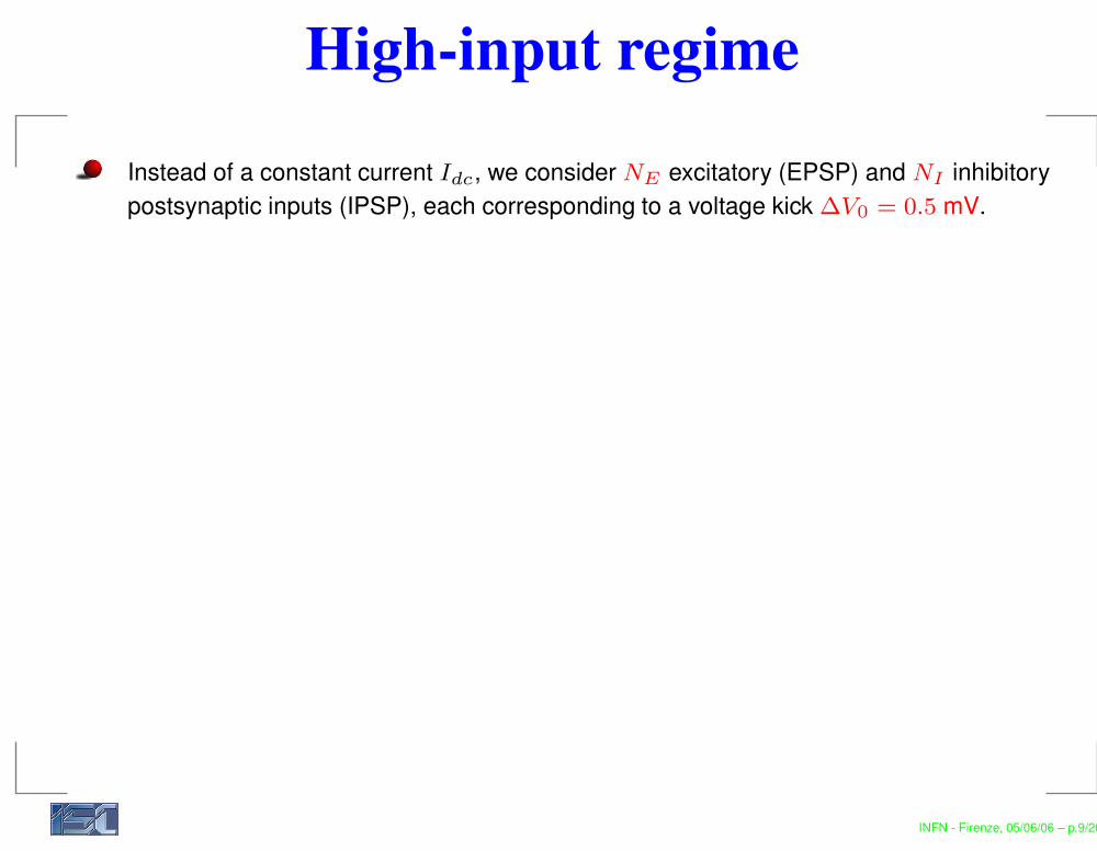
High-input regimeInstead of a constant current Idc, we consider NE excitatory (EPSP) and NI inhibitorypostsynaptic inputs (IPSP), each corresponding to a voltage kick ∆V0 = 0.5 mV.
These inputs originate from neurons emitting Poissonian spike trains with frequencyν = 100 Hz.This amounts to one excitatory (resp. inhibitory) Poissonian spike train with frequencyνE = Ne × ν ∼ 104 − 105 Hz (resp. νI = NI × ν) for Ne ∼ NI ∼ 100 − 1, 000.Firstly independent inputs are considered , and then also the effect of correlationsamong the inputs is analyzed.
INFN - Firenze, 05/06/06 – p.9/20

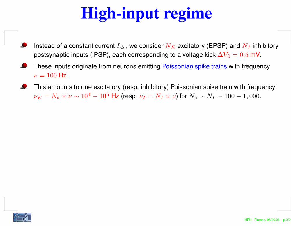
High-input regimeInstead of a constant current Idc, we consider NE excitatory (EPSP) and NI inhibitorypostsynaptic inputs (IPSP), each corresponding to a voltage kick ∆V0 = 0.5 mV.These inputs originate from neurons emitting Poissonian spike trains with frequencyν = 100 Hz.
This amounts to one excitatory (resp. inhibitory) Poissonian spike train with frequencyνE = Ne × ν ∼ 104 − 105 Hz (resp. νI = NI × ν) for Ne ∼ NI ∼ 100 − 1, 000.Firstly independent inputs are considered , and then also the effect of correlationsamong the inputs is analyzed.
INFN - Firenze, 05/06/06 – p.9/20
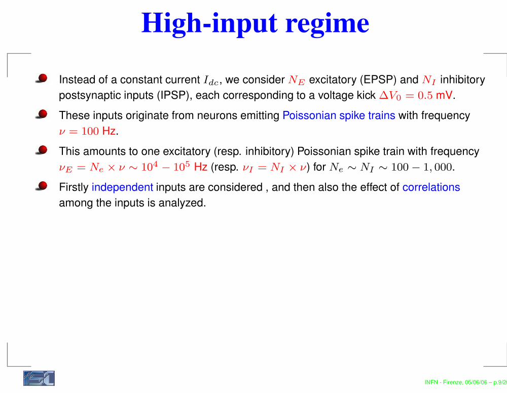
High-input regimeInstead of a constant current Idc, we consider NE excitatory (EPSP) and NI inhibitorypostsynaptic inputs (IPSP), each corresponding to a voltage kick ∆V0 = 0.5 mV.These inputs originate from neurons emitting Poissonian spike trains with frequencyν = 100 Hz.This amounts to one excitatory (resp. inhibitory) Poissonian spike train with frequencyνE = Ne × ν ∼ 104 − 105 Hz (resp. νI = NI × ν) for Ne ∼ NI ∼ 100 − 1, 000.
Firstly independent inputs are considered , and then also the effect of correlationsamong the inputs is analyzed.
INFN - Firenze, 05/06/06 – p.9/20
High-input regimeInstead of a constant current Idc, we consider NE excitatory (EPSP) and NI inhibitorypostsynaptic inputs (IPSP), each corresponding to a voltage kick ∆V0 = 0.5 mV.These inputs originate from neurons emitting Poissonian spike trains with frequencyν = 100 Hz.This amounts to one excitatory (resp. inhibitory) Poissonian spike train with frequencyνE = Ne × ν ∼ 104 − 105 Hz (resp. νI = NI × ν) for Ne ∼ NI ∼ 100 − 1, 000.Firstly independent inputs are considered , and then also the effect of correlationsamong the inputs is analyzed.
INFN - Firenze, 05/06/06 – p.9/20

High-input regimeInstead of a constant current Idc, we consider NE excitatory (EPSP) and NI inhibitorypostsynaptic inputs (IPSP), each corresponding to a voltage kick ∆V0 = 0.5 mV.These inputs originate from neurons emitting Poissonian spike trains with frequencyν = 100 Hz.This amounts to one excitatory (resp. inhibitory) Poissonian spike train with frequencyνE = Ne × ν ∼ 104 − 105 Hz (resp. νI = NI × ν) for Ne ∼ NI ∼ 100 − 1, 000.Firstly independent inputs are considered , and then also the effect of correlationsamong the inputs is analyzed.
At these frequencies the net input spike count within a temporal window ∆T (≥ 1 msec) isessentially Gaussian distributed and it can be characterized by its averageµ = ν(NE − NI)∆T and variance V = ν(NE + NI)∆T = νσ2∆T .
The response of the neuron is examined for fixed average input currentI = C∆V0ν(NE − NI) by varying only σ and therefore the standard deviation of the noise.
INFN - Firenze, 05/06/06 – p.9/20
Statistical and dynamical indicators
0 10 20 30 40t (ms)
-80
-60
-40
-20
0
20
40
V(t)
(mV
) . . .
ISI0 20 40 60 80 100 120
t (ms)
-0.2
0
0.2
0.4
0.6
0.8
1
C(t)
<I>=5µA/cm2 σ=26.46
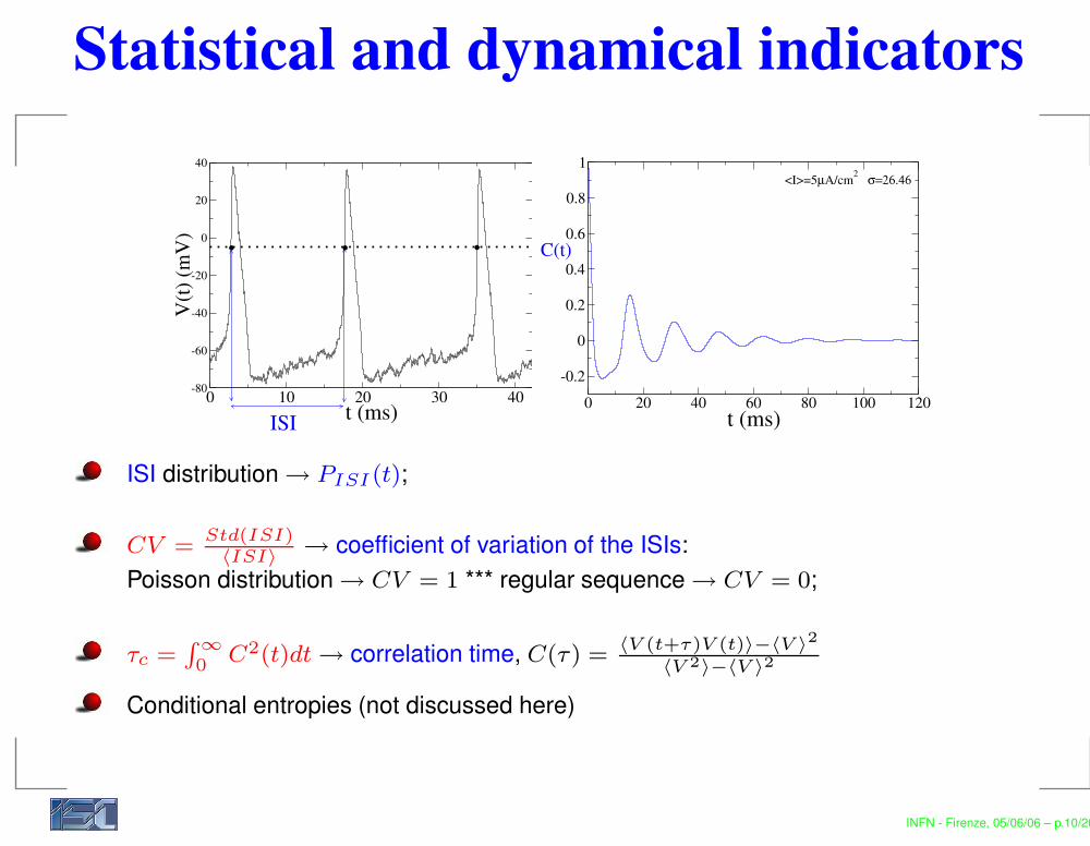
ISI distribution → PISI (t);
CV =Std(ISI)〈ISI〉
→ coefficient of variation of the ISIs:Poisson distribution → CV = 1 *** regular sequence → CV = 0;
τc =R ∞0 C2(t)dt → correlation time, C(τ) =
〈V (t+τ)V (t)〉−〈V 〉2
〈V 2〉−〈V 〉2
Conditional entropies (not discussed here)
INFN - Firenze, 05/06/06 – p.10/20

Response of the silent neuronThe HH neuron is in the silent state, i.e. the average input current I is smaller than ISN .
0 50 100 150σ
0
20
40
60
80
ν out (H
z)
0 0.1 0.2
1/σ2
10-4
10-2
100
102
ν out(H
z)
<I> = 5 µA/cm2
0 100 200 300 400t (ms)
10-4
10-3
10-2
10-1 PISI(t) σ=4.6
0 20 40 60 80 100t (ms)
0.001
0.01
0.1
P ISI(t)
σ=12.3
0 10 20 30 40t (ms)
0.001
0.01
0.1
P ISI(t)
σ=100.0
INFN - Firenze, 05/06/06 – p.11/20
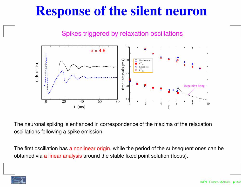
Response of the silent neuronSpikes triggered by relaxation oscillations
0 20 40 60 80t (ms)
(arb
. uni
ts)
σ = 4.6
0 2 4 6 8 10I
15
20
25
30
35
time
inte
rval
s (m
s) Nonlinear osc.t(1)
ISILinear osc.t(2)
ISI
Repetitive firing
The neuronal spiking is enhanced in correspondence of the maxima of the relaxationoscillations following a spike emission.
The first oscillation has a nonlinear origin, while the period of the subsequent ones can beobtained via a linear analysis around the stable fixed point solution (focus).
INFN - Firenze, 05/06/06 – p.11/20

Response of the silent neuronFiring activated by noise
Two mechanisms compete:
the HH dynamics tends to relax towards the rest state;noise fluctuations lead the system towards an excitation threshold.
The dynamics of V (t) resembles the overdamped dynamics of a particle in a potential wellunder the influence of thermal fluctuations, and the firing times can be expressed in terms ofthe Kramers expression (for sufficiently small noise)
ta ∝ eWS/σ2
the time distribution is Poissonian (CV = 1).
0 2 4 6 8 10 12I (µA/cm2)
0
50
100
150
W
Rest stateOscillatory state
Silence Bistability Firing
for σ <√
WS → Activation Processfor σ >
√WS → Diffusive Dynamics
INFN - Firenze, 05/06/06 – p.11/20

Response of the silent neuronHigh noise limit
The effect of noise fluctuations on the neuron dynamics is twofold:a constant current I driving the system;a stochastic term with zero average.
The dynamics of V (t) can therefore be described in terms of a Langevin process with a driftand the distribution of the first passage times is given by the inverse Gaussian distribution:
f(t) =α
p
2πβt3e−
(t−α)2
2βt
In this case the coefficient of variation shouldbe given by
CV ∝ σ
(I + I0)√
< ISI >
0 2 4 6 8 10 12 I (µA/cm2)
0.6
0.8
1
1.2 R*<ISI>1/2 (ms1/2)
INFN - Firenze, 05/06/06 – p.11/20
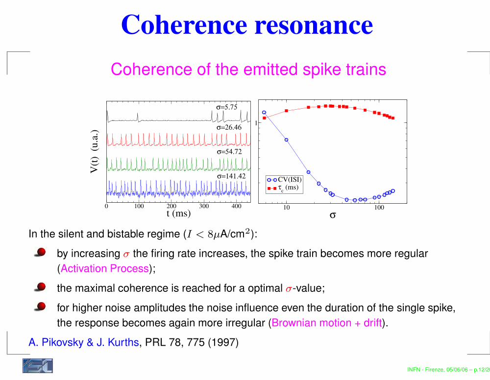
Coherence resonanceCoherence of the emitted spike trains
0 100 200 300 400t (ms)
V(t)
(u.
a.)
σ=5.75
σ=26.46
σ=54.72
σ=141.42
10 100σ
1
CV(ISI)τc (ms)
In the silent and bistable regime (I < 8µA/cm2):by increasing σ the firing rate increases, the spike train becomes more regular(Activation Process);the maximal coherence is reached for a optimal σ-value;for higher noise amplitudes the noise influence even the duration of the single spike,the response becomes again more irregular (Brownian motion + drift).
A. Pikovsky & J. Kurths, PRL 78, 775 (1997)
INFN - Firenze, 05/06/06 – p.12/20

Coherence resonance
The system is characterized by two characteristic times → ISI ≡ T = ta + te :ta=activation time → time needed to excite the system;te=excursion time → duration of the spike (excited state).
CV (T ) can be splitted in two contributionsCV (T )2 = CV (ta)2 <ta>2
<T>2 + CV (te)2<te>2
<T>2 = R21(ta) + R2
2(te)
R21(ta) decreases with σ, while R2
2(te) increases → minimum in CV (T )
B. Lindner et al., Phys Rep. 392 (2004) 321-424
INFN - Firenze, 05/06/06 – p.12/20
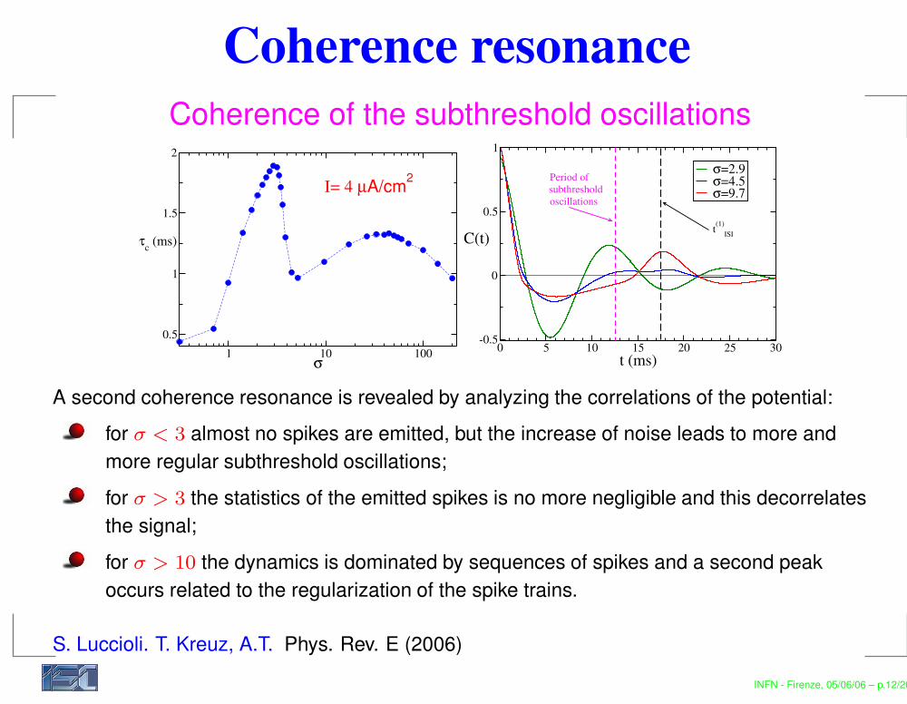
Coherence resonanceCoherence of the subthreshold oscillations
1 10 100σ
0.5
1
1.5
2
τc (ms)
I= 4 µA/cm2
0 5 10 15 20 25 30t (ms)
-0.5
0
0.5
1
σ=2.9σ=4.5σ=9.7
C(t)
Period ofsubthresholdoscillations
t(1)ISI
A second coherence resonance is revealed by analyzing the correlations of the potential:for σ < 3 almost no spikes are emitted, but the increase of noise leads to more andmore regular subthreshold oscillations;for σ > 3 the statistics of the emitted spikes is no more negligible and this decorrelatesthe signal;for σ > 10 the dynamics is dominated by sequences of spikes and a second peakoccurs related to the regularization of the spike trains.
S. Luccioli. T. Kreuz, A.T. Phys. Rev. E (2006)
INFN - Firenze, 05/06/06 – p.12/20
Correlations via common drive
The correlation between two input spike trains originating from neuron i
and j is measured in terms of the Pearson correlation coefficient :
ρ =< (ni − 〈ni〉)(nj − 〈nj〉) >
s2
where n is the number of input spikes in a time window ∆T and s2 itsvariance.
Correlations among either excitatory or inhibitory inputs are considered inthe balanced case NE = NI ≡ N (< I >≡ 0).
M.N. Shadlen & W.T. Newsome (1998) – E. Salinas & J. Sejnowski (2000)
INFN - Firenze, 05/06/06 – p.13/20
Correlations via common driveThe superposition of N correlated (ρ) Poissonian spike trains withrate ν0 gives rise to a sequence of kicks of variable amplitude(binomially distributed) and with ISIs Poissonian distributed with rateν0/ρ;For correlated kicks: average amplitude < ∆V >= ρN∆V0 andaverage frequency νc = ν0/ρ;For uncorrelated kicks: frequency=Nν0 and constant amplitude=∆V0.The noise variance is influenced by correlations σ ∼< δV >2 ×νc
while < I >≡ 0 not.
The uncorrelated spike trains can be assimilated to an almost continuousbackground that renormalizes the input current, while the correlated kickscan be seen as rare events of large amplitude.
INFN - Firenze, 05/06/06 – p.13/20
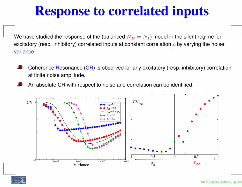
Response to correlated inputsWe have studied the response of the (balanced NE = NI ) model in the silent regime forexcitatory (resp. inhibitory) correlated inputs at constant correlation ρ by varying the noisevariance.
Coherence Resonance (CR) is observed for any excitatory (resp. inhibitory) correlationat finite noise amplitude.An absolute CR with respect to noise and correlation can be identified.
1e+05 1e+06 1e+07 1e+08Variance
0.1
1CV ρEE=1.0 ρEE= 0.5 ρEE= 0 = ρII ρII = 0.5 ρII = 1.0
1 0.5 0 0.5 1
CVmin
ρeeρii
INFN - Firenze, 05/06/06 – p.14/20
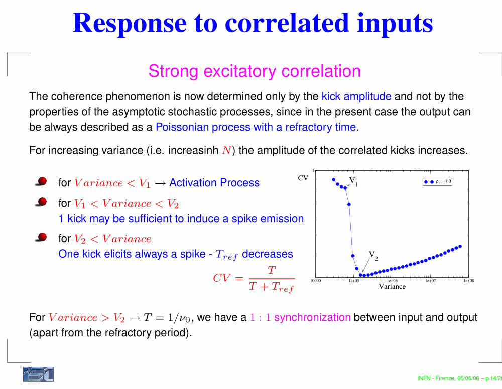
Response to correlated inputsStrong excitatory correlation
The coherence phenomenon is now determined only by the kick amplitude and not by theproperties of the asymptotic stochastic processes, since in the present case the output canbe always described as a Poissonian process with a refractory time.
For increasing variance (i.e. increasinh N ) the amplitude of the correlated kicks increases.
10000 1e+05 1e+06 1e+07 1e+08Variance
1
CV ρEE=1.0V1
V2
for V ariance < V1 → Activation Processfor V1 < V ariance < V2
1 kick may be sufficient to induce a spike emissionfor V2 < V ariance
One kick elicits always a spike - Tref decreases
CV =T
T + Tref
For V ariance > V2 → T = 1/ν0, we have a 1 : 1 synchronization between input and output(apart from the refractory period).
INFN - Firenze, 05/06/06 – p.14/20
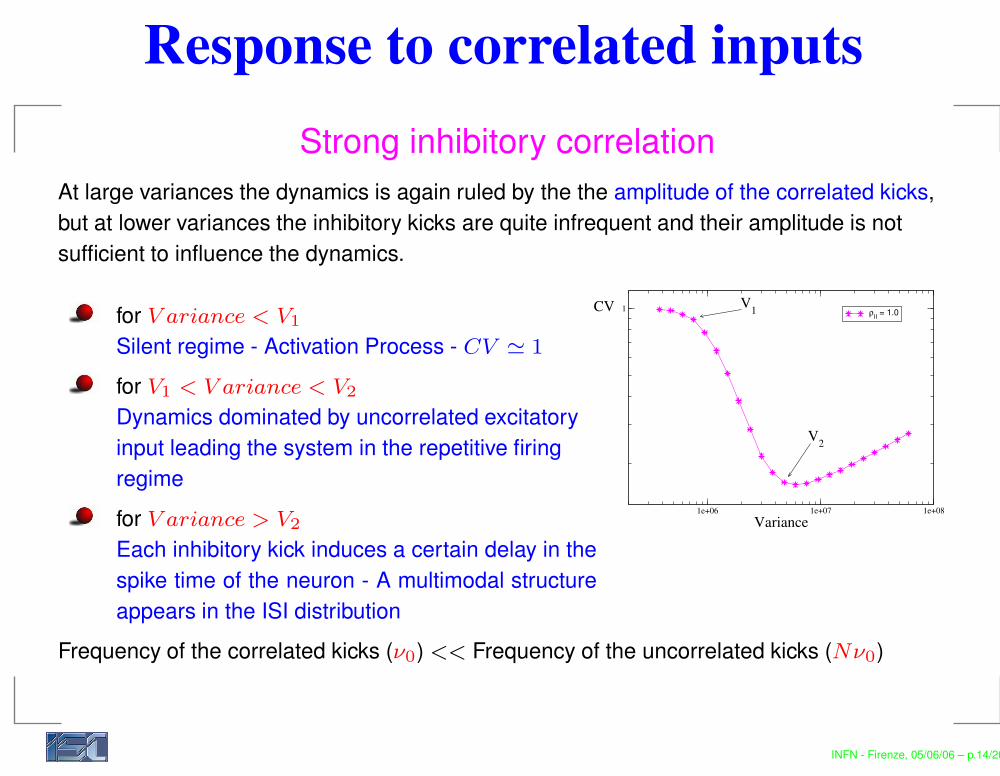
Response to correlated inputsStrong inhibitory correlation
At large variances the dynamics is again ruled by the the amplitude of the correlated kicks,but at lower variances the inhibitory kicks are quite infrequent and their amplitude is notsufficient to influence the dynamics.
1e+06 1e+07 1e+08Variance
1CV ρII = 1.0V1
V2
for V ariance < V1
Silent regime - Activation Process - CV ' 1
for V1 < V ariance < V2
Dynamics dominated by uncorrelated excitatoryinput leading the system in the repetitive firingregimefor V ariance > V2
Each inhibitory kick induces a certain delay in thespike time of the neuron - A multimodal structureappears in the ISI distribution
Frequency of the correlated kicks (ν0) << Frequency of the uncorrelated kicks (Nν0)
INFN - Firenze, 05/06/06 – p.14/20
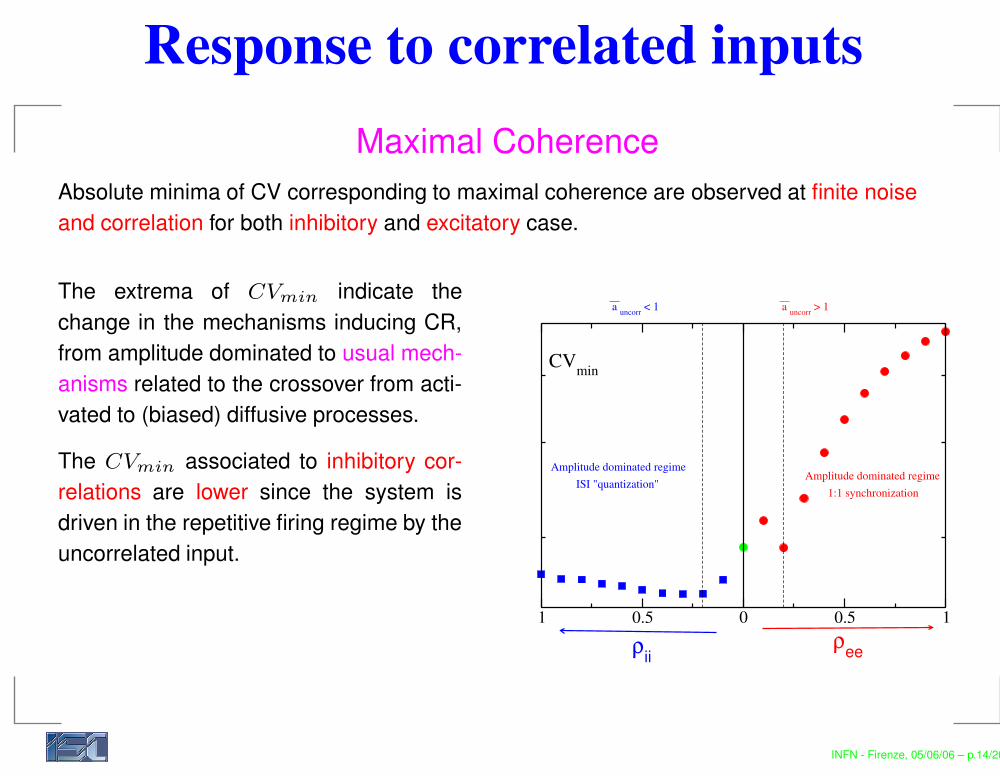
Response to correlated inputsMaximal Coherence
Absolute minima of CV corresponding to maximal coherence are observed at finite noiseand correlation for both inhibitory and excitatory case.
The extrema of CVmin indicate thechange in the mechanisms inducing CR,from amplitude dominated to usual mech-anisms related to the crossover from acti-vated to (biased) diffusive processes.
The CVmin associated to inhibitory cor-relations are lower since the system isdriven in the repetitive firing regime by theuncorrelated input.
1 0.5 0 0.5 1
CVmin
ρeeρii
Amplitude dominated regimeAmplitude dominated regime
1:1 synchronizationISI "quantization"
a uncorr < 1 a uncorr > 1
INFN - Firenze, 05/06/06 – p.14/20
ConclusionsUncorrelated stochastic inputs
The neuronal firing, induced by the stochastic inputs, can be interpreted as anactivation process at low variances (σ), while for large σ this process becomesessentially diffusive;at low noise, beside of the exponential tail, the ISI distributions reveal a multimodalstructure due to spiking triggered by relaxation oscillations towards the rest state;coherence resonance can be observed in a large interval of currents in the silentand bistable regime whenever WS > WO;a second coherence resonance (associated to subthreshold oscillations) coexistswith the usual one;
Correlated stochastic inputs
new mechanisms for the coherence resonance have been reported at highexcitatory and inhibitory correlations;maximal coherence can be induced by an optimal combination of noise andcorrelation
INFN - Firenze, 05/06/06 – p.15/20
Credits
Stefano Luccioli - MSc in Physics (2004-2005)Dynamics of realistic single neuronal models
Thomas Kreuz - Marie Curie Fellow (2005-2006)Dynamical Entropies in Assemblies of Neurons
http://www.fi.isc.cnr.it/users/alessandro.torcini/neurores.html
INFN - Firenze, 05/06/06 – p.16/20

L’esperimento di Voltage-ClampL’esperimento di blocco del voltaggio (voltage clamp) consiste nell’inserire nell’assone delcalamaro due elettrodi (fili di argento), uno che serve a misurare Vm e l’altro per trametterecorrente dentro l’assone cosí da mantenere (retroattivamente) Vm costante.
Effetti positivi del voltage clamp:elimina la corrente capacitivaIC ≡ 0 ;si possono misurare ledipendenze temporali dellevarie correnti (conduttanze) aVm costante;inserendo gli elettrodi si haanche uno space-clamp cioétutta la lunghezza dello assoneha lo stesso Vm
HH were able to measure separately the different currents thanks to pharmacologicalproducts able to block selectively the different ionic channels.
INFN - Firenze, 05/06/06 – p.17/20
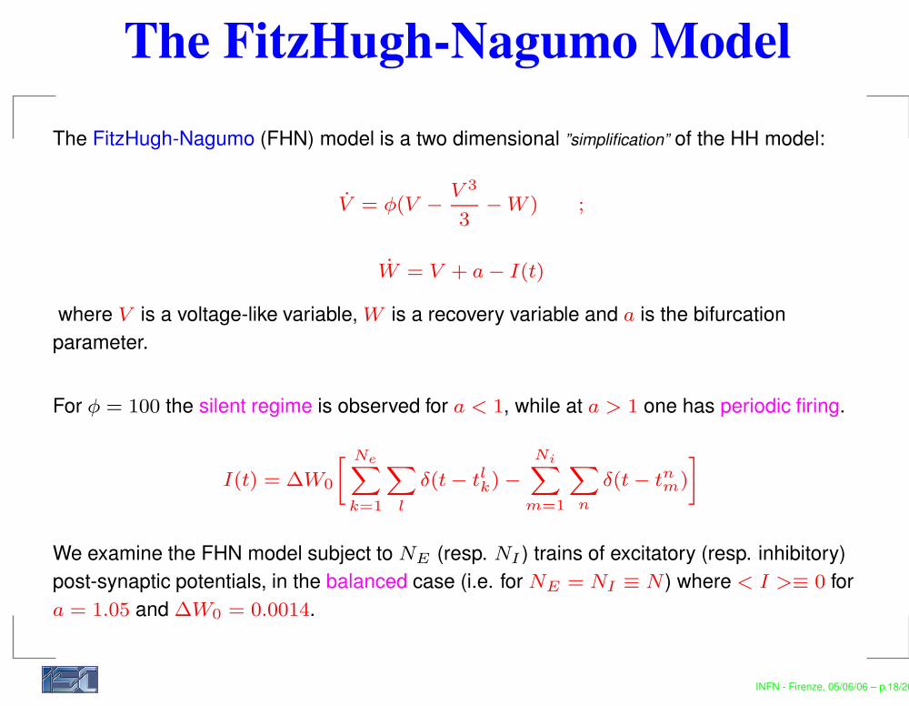
The FitzHugh-Nagumo ModelThe FitzHugh-Nagumo (FHN) model is a two dimensional ”simplification” of the HH model:
V = φ(V − V 3
3− W ) ;
W = V + a − I(t)
where V is a voltage-like variable, W is a recovery variable and a is the bifurcationparameter.
For φ = 100 the silent regime is observed for a < 1, while at a > 1 one has periodic firing.
I(t) = ∆W0
» NeX
k=1
X
l
δ(t − tlk) −NiX
m=1
X
n
δ(t − tnm)
–
We examine the FHN model subject to NE (resp. NI ) trains of excitatory (resp. inhibitory)post-synaptic potentials, in the balanced case (i.e. for NE = NI ≡ N ) where < I >≡ 0 fora = 1.05 and ∆W0 = 0.0014.
INFN - Firenze, 05/06/06 – p.18/20

Correlations via common driveCorrelations only among excitatory or inhibitory inputs are considered in the balancedcase NE = NI ≡ N ;
The superposition of N correlated (ρ) Poissonian spike trains with rate ν0 gives rise toa sequence of kicks of variable amplitude (binomially distributed) and with ISIsPoissonian distributed with rate ν0/ρ;The average input is not influenced by correlations < I >≡ 0, instead the noisevariance is ∆V 2ν0[N2ρ + N(1 − ρ) + N ];For correlated kicks: average amplitude=ρN∆V and average frequency=ν0/ρ;For uncorrelated kicks: frequency=Nν0 and amplitude= ∆V .
INFN - Firenze, 05/06/06 – p.19/20

Correlations via common driveCorrelations only among excitatory or inhibitory inputs are considered in the balancedcase NE = NI ≡ N ;The superposition of N correlated (ρ) Poissonian spike trains with rate ν0 gives rise toa sequence of kicks of variable amplitude (binomially distributed) and with ISIsPoissonian distributed with rate ν0/ρ;
The average input is not influenced by correlations < I >≡ 0, instead the noisevariance is ∆V 2ν0[N2ρ + N(1 − ρ) + N ];For correlated kicks: average amplitude=ρN∆V and average frequency=ν0/ρ;For uncorrelated kicks: frequency=Nν0 and amplitude= ∆V .
INFN - Firenze, 05/06/06 – p.19/20
Correlations via common driveCorrelations only among excitatory or inhibitory inputs are considered in the balancedcase NE = NI ≡ N ;The superposition of N correlated (ρ) Poissonian spike trains with rate ν0 gives rise toa sequence of kicks of variable amplitude (binomially distributed) and with ISIsPoissonian distributed with rate ν0/ρ;The average input is not influenced by correlations < I >≡ 0, instead the noisevariance is ∆V 2ν0[N2ρ + N(1 − ρ) + N ];
For correlated kicks: average amplitude=ρN∆V and average frequency=ν0/ρ;For uncorrelated kicks: frequency=Nν0 and amplitude= ∆V .
INFN - Firenze, 05/06/06 – p.19/20
Correlations via common driveCorrelations only among excitatory or inhibitory inputs are considered in the balancedcase NE = NI ≡ N ;The superposition of N correlated (ρ) Poissonian spike trains with rate ν0 gives rise toa sequence of kicks of variable amplitude (binomially distributed) and with ISIsPoissonian distributed with rate ν0/ρ;The average input is not influenced by correlations < I >≡ 0, instead the noisevariance is ∆V 2ν0[N2ρ + N(1 − ρ) + N ];For correlated kicks: average amplitude=ρN∆V and average frequency=ν0/ρ;
For uncorrelated kicks: frequency=Nν0 and amplitude= ∆V .
INFN - Firenze, 05/06/06 – p.19/20
Correlations via common driveCorrelations only among excitatory or inhibitory inputs are considered in the balancedcase NE = NI ≡ N ;The superposition of N correlated (ρ) Poissonian spike trains with rate ν0 gives rise toa sequence of kicks of variable amplitude (binomially distributed) and with ISIsPoissonian distributed with rate ν0/ρ;The average input is not influenced by correlations < I >≡ 0, instead the noisevariance is ∆V 2ν0[N2ρ + N(1 − ρ) + N ];For correlated kicks: average amplitude=ρN∆V and average frequency=ν0/ρ;For uncorrelated kicks: frequency=Nν0 and amplitude= ∆V .
The correlation between two input spike trains originating from neuron i and j is measured interms of the Pearson correlation coefficient :
ρ =< (ni − 〈ni〉)(nj − 〈nj〉) >
s2
where n is the number of spikes in a time window ∆T and s2 its variance. M.N. Shadlen &
W.T. Newsome (1998) – E. Salinas & J. Sejnowski (2000)INFN - Firenze, 05/06/06 – p.19/20
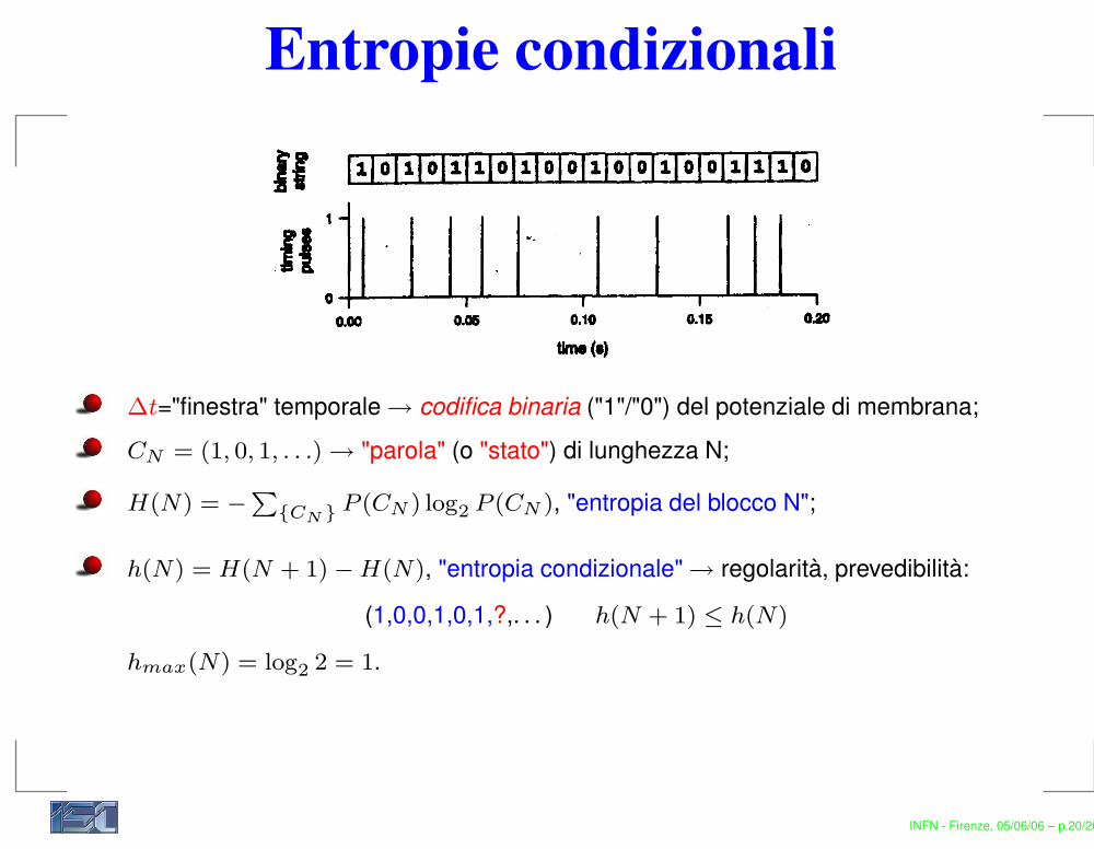
Entropie condizionali
∆t="finestra" temporale → codifica binaria ("1"/"0") del potenziale di membrana;CN = (1, 0, 1, . . .) → "parola" (o "stato") di lunghezza N;
H(N) = −P
{CN} P (CN ) log2 P (CN ), "entropia del blocco N";
h(N) = H(N + 1) − H(N), "entropia condizionale" → regolarità, prevedibilità:
(1,0,0,1,0,1,?,. . . ) h(N + 1) ≤ h(N)
hmax(N) = log2 2 = 1.
INFN - Firenze, 05/06/06 – p.20/20