response optimisation sloptim gsg
TRANSCRIPT
Simulink® ResponseOptimization
For Use with Simulink®
Modeling
Simulation
Implementation
Getting StartedVersion 3
How to Contact The MathWorks
www.mathworks.com Webcomp.soft-sys.matlab Newsgroupwww.mathworks.com/contact_TS.html Technical Support
[email protected] Product enhancement [email protected] Bug [email protected] Documentation error [email protected] Order status, license renewals, [email protected] Sales, pricing, and general information
508-647-7000 (Phone)
508-647-7001 (Fax)
The MathWorks, Inc.3 Apple Hill DriveNatick, MA 01760-2098For contact information about worldwide offices, see the MathWorks Web site.
Getting Started with Simulink Response Optimization
© COPYRIGHT 2004–2006 The MathWorks, Inc.The software described in this document is furnished under a license agreement. The software may be usedor copied only under the terms of the license agreement. No part of this manual may be photocopied orreproduced in any form without prior written consent from The MathWorks, Inc.
FEDERAL ACQUISITION: This provision applies to all acquisitions of the Program and Documentationby, for, or through the federal government of the United States. By accepting delivery of the Program orDocumentation, the government hereby agrees that this software or documentation qualifies as commercialcomputer software or commercial computer software documentation as such terms are used or definedin FAR 12.212, DFARS Part 227.72, and DFARS 252.227-7014. Accordingly, the terms and conditions ofthis Agreement and only those rights specified in this Agreement, shall pertain to and govern the use,modification, reproduction, release, performance, display, and disclosure of the Program and Documentationby the federal government (or other entity acquiring for or through the federal government) and shallsupersede any conflicting contractual terms or conditions. If this License fails to meet the government’sneeds or is inconsistent in any respect with federal procurement law, the government agrees to return theProgram and Documentation, unused, to The MathWorks, Inc.
Trademarks
MATLAB, Simulink, Stateflow, Handle Graphics, Real-Time Workshop, and xPC TargetBoxare registered trademarks, and SimBiology, SimEvents, and SimHydraulics are trademarks ofThe MathWorks, Inc.
Other product or brand names are trademarks or registered trademarks of their respectiveholders.
Patents
The MathWorks products are protected by one or more U.S. patents. Please seewww.mathworks.com/patents for more information.

Revision HistoryJune 2004 First printing New for Version 2.0 (Release 14) (Renamed from Nonlinear
Control Design Blockset User’s Guide)October 2004 Online only Revised for Version 2.1 (Release 14SP1)March 2005 Online only Revised for Version 2.2 (Release 14SP2)September 2005 Online only Revised for Version 2.3 (Release 14SP3)March 2006 Second printing Revised for Version 3.0 (Release 2006a)September 2006 Online only Revised for Version 3.1 (Release 2006b)

Contents
What Is Simulink Response Optimization?
1Introduction . . . . . . . . . . . . . . . . . . . . . . . . . . . . . . . . . . . . . . 1-2
Tuning within Simulink Models . . . . . . . . . . . . . . . . . . . . . . 1-2Tuning within a SISO Design Task . . . . . . . . . . . . . . . . . . . 1-3Applications . . . . . . . . . . . . . . . . . . . . . . . . . . . . . . . . . . . . . . 1-3
System Requirements . . . . . . . . . . . . . . . . . . . . . . . . . . . . . . 1-5
Upgrading from the Nonlinear Control DesignBlockset . . . . . . . . . . . . . . . . . . . . . . . . . . . . . . . . . . . . . . . . 1-5
Using the Documentation . . . . . . . . . . . . . . . . . . . . . . . . . . 1-6Expected Background . . . . . . . . . . . . . . . . . . . . . . . . . . . . . . 1-6How to Use This Guide . . . . . . . . . . . . . . . . . . . . . . . . . . . . . 1-6Online Documentation . . . . . . . . . . . . . . . . . . . . . . . . . . . . . 1-6
Response Optimization Tutorial
2Quick Start — Time Domain Response Optimization of
Simulink Models . . . . . . . . . . . . . . . . . . . . . . . . . . . . . . . . 2-2
Quick Start — Mixed Time and Frequency DomainResponse Optimization . . . . . . . . . . . . . . . . . . . . . . . . . . 2-4
Simple Control Design Example . . . . . . . . . . . . . . . . . . . . . 2-6Simulink Response Optimization Startup . . . . . . . . . . . . . . 2-6Adjusting Constraints . . . . . . . . . . . . . . . . . . . . . . . . . . . . . . 2-7Specifying Tuned Parameters . . . . . . . . . . . . . . . . . . . . . . . 2-11Running the Optimization . . . . . . . . . . . . . . . . . . . . . . . . . . 2-13Tracking a Signal . . . . . . . . . . . . . . . . . . . . . . . . . . . . . . . . . 2-15
v

Adding Uncertainty . . . . . . . . . . . . . . . . . . . . . . . . . . . . . . . . 2-18Saving the Project . . . . . . . . . . . . . . . . . . . . . . . . . . . . . . . . . 2-21
Frequency Domain Response Optimization Example . . 2-23Creating an LTI Plant Model . . . . . . . . . . . . . . . . . . . . . . . . 2-23Creating Design and Analysis Plots . . . . . . . . . . . . . . . . . . . 2-24Creating a Response Optimization Task . . . . . . . . . . . . . . . 2-28Selecting Tunable Compensator Elements . . . . . . . . . . . . . 2-29Adding Design Requirements . . . . . . . . . . . . . . . . . . . . . . . . 2-30Optimizing the System’s Response . . . . . . . . . . . . . . . . . . . 2-39Creating and Displaying the Closed-Loop System . . . . . . . 2-42
Physical Modeling Example . . . . . . . . . . . . . . . . . . . . . . . . 2-45Opening the Hydraulic Cylinder Model . . . . . . . . . . . . . . . . 2-45Adjusting Constraints . . . . . . . . . . . . . . . . . . . . . . . . . . . . . . 2-47Specifying Tuned Parameters . . . . . . . . . . . . . . . . . . . . . . . 2-52Running the Optimization . . . . . . . . . . . . . . . . . . . . . . . . . . 2-53Changing Optimization Settings . . . . . . . . . . . . . . . . . . . . . 2-54Finding a Maximally Feasible Solution . . . . . . . . . . . . . . . . 2-57
Response Optimization Using Functions
3Control Design Example Using Functions . . . . . . . . . . . . 3-2
Choosing Signals to Constrain . . . . . . . . . . . . . . . . . . . . . . . 3-2Creating an Optimization Project . . . . . . . . . . . . . . . . . . . . 3-2Properties of a Response Optimization Project . . . . . . . . . . 3-4Running the Optimization . . . . . . . . . . . . . . . . . . . . . . . . . . 3-10
Troubleshooting
4Common Questions About Response Optimization . . . . 4-2
Questions . . . . . . . . . . . . . . . . . . . . . . . . . . . . . . . . . . . . . . . . 4-2
vi Contents

Index
vii

viii Contents

1
What Is Simulink ResponseOptimization?
Introduction (p. 1-2) Introduction to the key features ofSimulink® Response Optimization
System Requirements (p. 1-5) Required and related products
Upgrading from the NonlinearControl Design Blockset (p. 1-5)
Information on upgrading NCDmodels for use with SimulinkResponse Optimization
Using the Documentation (p. 1-6) Expected background, how to usethis guide, and other documentationsources

1 What Is Simulink Response Optimization?
IntroductionSimulink Response Optimization provides a graphical user interface (GUI)to assist in the tuning and optimization of control systems and physicalsystems. With this product, you can either directly tune response signalswithin Simulink models or tune responses of LTI systems within a SISODesign Task (requires the Control System Toolbox).
Tuning within Simulink ModelsYou can tune parameters within a nonlinear Simulink model to meettime-domain performance requirements by graphically constraining signalswithin a time-domain window or tracking and closely matching a referencesignal.
You can tune any number of Simulink variables including scalars, vectors,and matrices. In addition, you can place uncertainty bounds on othervariables in the model for robust design. Simulink Response Optimizationmakes attaining performance objectives and optimizing tuned parameters anintuitive and easy process.
To use Simulink Response Optimization to directly tune Simulink models,you need only to include a special block, the Signal Constraint block, inyour Simulink diagram. Just connect the block to any signal in the model tosignify that you want to place some kind of constraint on the signal. SimulinkResponse Optimization automatically converts time-domain constraintsinto a constrained optimization problem and then solves the problemusing optimization routines taken from the Optimization Toolbox or theGenetic Algorithm and Direct Search Toolbox. The constrained optimizationproblem formulated by Simulink Response Optimization iteratively calls forsimulations of the Simulink system, compares the results of the simulationswith the constraint objectives, and uses gradient methods to adjust tunedparameters to better meet the objectives.
Two additional blocks, CRMS and DRMS, compute the continuous anddiscrete cumulative root mean square values of signals. Use them with theSignal Constraint block to optimize the cumulative root mean square ofsignals in your model.
1-2

Introduction
Tuning within a SISO Design TaskWhen you have the Control System Toolbox installed, you can designcompensators for control systems by tuning compensator elements orparameters within a SISO Design Task in the Control and Estimation ToolsManager. You can tune any elements or parameters, such as poles, zeros, andgains, within any compensators in the system to optimize the responses ofboth open and closed loops.
Optimize the responses of systems in the SISO Design Task to meet bothtime- and frequency-domain performance requirements by graphicallyconstraining signals:
• Add frequency-domain design requirements to plots such as root-locus,Nichols, and Bode in the SISO Design Task graphical tuning editor calledSISO Design Tool.
• Add time-domain design requirements to plots such as step or impulseresponse (when displayed within the LTI Viewer as part of a SISO DesignTask).
You can use response optimization within a SISO Design Task in the Controland Estimation Tools Manager to tune both command-line LTI models as wellas Simulink models:
• Create an LTI model using the Control System Toolbox command-linefunctions and use the sisotool function to create a SISO Design Taskfor the model.
• Use a Simulink Compensator Design task (from the product SimulinkControl Design) to automatically analyze the model and then create aSISO Design Task for a linearized version of the model. You can then usethe response optimization tools within the SISO Design Task to tune theresponse of the linearized Simulink model.
When using response optimization within a SISO Design Task you cannot adduncertainty to system parameters.
ApplicationsYou can use Simulink Response Optimization for a variety of applications.Possible uses include
1-3
1 What Is Simulink Response Optimization?
• Designing and optimizing control systems by tuning compensator elementssuch as poles, zeros, and gains.
• Designing physical systems by adjusting parameters in your system. Forexample, adjust the dimensions of physical devices such as robot arms orhydraulic pistons, tune properties of materials such as thermal emissivity,etc.
• Closely tracking a reference, or desired, signal (using the Signal Constraintblock only).
• Optimizing responses for systems that include physical actuation limitsand constraints on state/variable values.
• Minimizing the energy in a system by minimizing the root-mean-squaresignal.
• Including uncertainty in your parameter values to take into accountimperfect knowledge of certain physical parameters in your model (usingthe Signal Constraint block only).
1-4
System Requirements
System RequirementsSimulink Response Optimization has the same system requirementsas MATLAB®. Refer to the MATLAB documentation for details.For a list of required and related products, see the SimulinkResponse Optimization product page on the MathWorks Web site athttp://www.mathworks.com/products/simresponse/.
Upgrading from the Nonlinear Control Design BlocksetSimulink Response Optimization replaces the Nonlinear Control Design(NCD) Blockset. For information on upgrading from the Nonlinear ControlDesign Blockset, refer to the Release Notes. In addition, the ncdupdatereference page has detailed information on updating NCD models.
1-5
1 What Is Simulink Response Optimization?
Using the Documentation
Expected BackgroundUsers of this guide should be familiar with dynamic systems design andanalysis, and have experience creating Simulink models.
How to Use This GuideTo get started using Simulink Response Optimization, read Chapter 2,“Response Optimization Tutorial” which introduces the main product featuresand uses three simple examples to describe their use.
To use both time- and frequency-domain design requirements tooptimize the response of LTI systems in a SISO Design Task (requires theControl System Toolbox), read “Frequency Domain Response OptimizationExample” on page 2-23.
To perform response optimization using functions, read Chapter 3,“Response Optimization Using Functions”.
For advice on solving typical problems, read Chapter 4,“Troubleshooting”.
If you are upgrading from the Nonlinear Control Design (NCD)Blockset, read the Release Notes to learn about new features and how toconvert your NCD models for use with Simulink Response Optimization.
Online DocumentationFurther documentation is available online, including function and blockreferences, and detailed discussions on setting up and running a responseoptimization.
1-6
2
Response OptimizationTutorial
You can use Simulink Response Optimization to solve a wide variety ofcontrol and physical design problems by either inserting Signal Constraintblocks in your model or creating a SISO Design Task for your system, andthen using the graphical user interface (GUI) to specify constraints anddesign requirements for these signals and systems. You can specify tunedand optimization settings as well as uncertain parameters (with the SignalConstraint block only). To get started with Simulink Response Optimization,work through the three examples in this chapter or use the Quick Start guides.
Quick Start — Time DomainResponse Optimization of SimulinkModels (p. 2-2)
A brief outline of the responseoptimization process using timedomain requirements for Simulinkmodels
Quick Start — Mixed Time andFrequency Domain ResponseOptimization (p. 2-4)
A brief outline of the responseoptimization process using bothtime and frequency domain designrequirements
Simple Control Design Example(p. 2-6)
An example that tunes a singlesystem parameter to optimize aresponse signal
Frequency Domain ResponseOptimization Example (p. 2-23)
An example that tunes a system sothat its dynamics meet frequencydomain requirements
Physical Modeling Example (p. 2-45) An example that tunes multiplesystem parameters to optimizemultiple response signals
2 Response Optimization Tutorial
Quick Start — Time Domain Response Optimization ofSimulink Models
If you want to quickly get started using Simulink Response Optimizationfor time domain response optimization of Simulink models, this sectionsummarizes the response optimization process:
1 Make a model of your (nonlinear) system and controller using Simulink.Add input signals (e.g., steps, ramps, observed data) for which you knowwhat the desired output should look like.
2 Attach a Signal Constraint block to the signals you want to constrain. TheSimulink library srolib contains the Signal Constraint block. To openthe library, just type srolib at the MATLAB prompt or select SimulinkResponse Optimization from the Simulink Library Browser.
3 If the model’s parameters do not already exist in the MATLAB workspace,initialize these parameters in the workspace with a best first guess.
4 Double-click each Signal Constraint block in your system to open theSignal Constraint window for each constrained output. Choose a methodfor constraining the response signal by selecting Enforce signal boundsand/or Track reference signal at the bottom of the window.
5 Within the Signal Constraint window, constrain each signal by positioningconstraint bound segments and/or tracking a reference signal. You canposition constraint bound segments by clicking and dragging the segmentor right-clicking the segment and selecting Edit from the menu. Plotreference signals by selecting Goals > Desired Response from the SignalConstraint window and entering vectors of data for the reference signal.
6 Open the Tuned Parameters dialog box by selecting Optimization > TunedParameters within a Signal Constraint window. Click the Add button toadd parameters to the list. Select a parameter in the list to specify initialguesses and maximum and minimum values.
7 Optional: Open the Uncertain Parameters dialog box by selectingOptimization > Uncertain Parameters within a Signal Constraintwindow. Click the Add button to add parameters to the list. Choose a
2-2

Quick Start — Time Domain Response Optimization of Simulink Models
method and range for sampling the uncertain parameters and select whichresponses to optimize.
8 Optional: Save the project, including constraints, tuned parameters,uncertain parameters, and settings for optimization and simulation, to afile, to the MATLAB workspace, or to the model workspace by selectingFile > Save. You can retrieve previously saved projects by selectingFile > Load. To automatically save and reload the project with theSimulink model, select the check box at the bottom of the Save dialog box.Note that when saving the project, you are saving the entire optimizationproject, which might include several Signal Constraint blocks.
9 Click the Start button in the toolbar or select Start from the Optimizationmenu to optimize the response signal by adjusting the tuned parameters.The Optimization Progress window displays the new, optimized parametervalues.
2-3
2 Response Optimization Tutorial
Quick Start — Mixed Time and Frequency DomainResponse Optimization
This section outlines the response optimization process for linear systemswithin a SISO Design Task in the Control and Estimation Tools Managerusing both time and frequency domain design requirements:
1 Create and import a linear model into a SISO Design Task using oneof two methods:
• Create an LTI model of your system at the MATLAB command line anduse the sisotool function to create a SISO Design Tool for the model.
• Create a Simulink model and use a Simulink Compensator Design Taskwith the product Simulink Control Design to automatically linearize themodel and create a SISO Design Task for the linearized model.
2 Optional: Within the SISO Design Task node of the Control andEstimation Tools Manager, select the Architecture pane and then select acontrol architecture for your system.
3 Use the Graphical Tuning pane within the SISO Design Task nodeof the Control and Estimation Tools Manager to create any design plotsyou want to use to design the response of the system, such as root-locusdiagrams, Bode plots, etc. Use the Analysis Plots pane to create anyanalysis plots you want to use to view the system, such as step or impulseresponse plots.
4 Within the Automated Tuning pane select Optimization based tuningas the Design Method and then click the Optimize Compensatorsbutton to create a Response Optimization task within the Control andEstimation Tools Manager.
5 Within the Response Optimization node, select the Compensatorspane to select and configure the compensator elements you want to tuneduring the response optimization. Note that when optimizing responsesin a SISO Design Task, you cannot add uncertainty to parameters orcompensator elements.
6 Within the Design requirements pane of the Response Optimizationnode, select the design requirements you want the system to satisfy. To
2-4

Quick Start — Mixed Time and Frequency Domain Response Optimization
add a new design requirement to a design or analysis plot, click the Addnew design requirement button and then complete the New DesignRequirement dialog box.
7 Optional: To change the default optimization settings and configure themfor your problem, click the Optimization Options button within theOptimization pane.
8 Click the Start Optimization button within the Response Optimizationnode. The optimization progress results appear within the Optimizationpane. The Compensators pane contains the new, optimized compensatorelement values.
9 Optional: There are several options to export and save the results of theresponse optimization:
• To export the newly designed compensators to the MATLAB Workspaceor a MAT-file, select File > Workspace within the SISO Design Toolgraphical tuning window.
• To save the SISO Design task, including the Response Optimizationtask, select File > Save within the Control and Estimation ToolsManager.
• If you are designing compensators for a Simulink model, click theUpdate Simulink Block Parameters button within the SISO DesignTask node to write the newly designed compensators to the Simulinkmodel.
2-5

2 Response Optimization Tutorial
Simple Control Design ExampleResponse optimization of Simulink models using Simulink ResponseOptimization uses time-domain constraint bounds to represent lower andupper bounds on response signals. You can stretch, move, split, or openconstraint bounds in a variety of ways that are explained here and in theonline documentation. This section guides you through an example of how youmight perform control design directly in a Simulink model using SimulinkResponse Optimization. In this section, you will constrain a parameter tocontrol a second order SISO system via integral action, shown in the diagrambelow.
Specifically, the integral gain (Kint) should ensure that the closed loop systemmeets or exceeds the following performance specifications when you excitethe system with a unit step input:
• A maximum 10% overshoot
• A maximum 10-second rise time
• A maximum 30-second settling time
Because of the actuator limits and system transport delay, standard linearcontrol design techniques may not yield reliable results.
Simulink Response Optimization StartupThe Simulink model srotut1 contains the system shown above. Open thesystem by typing srotut1 at the MATLAB prompt.
You do not need to remodel any of your present Simulink systems to useSimulink Response Optimization. You need simply to
2-6
Simple Control Design Example
1 Attach a Signal Constraint block to all signals you want to constrain. Insrotut1, a Signal Constraint block (square block with a step responseicon) is attached to the plant output.
2 Add input signals to the system, for which you know what the outputshould look like. In srotut1, the input is a step since the desired stepresponse characteristics of the system are known.
3 Change the model’s Stop time to the desired value. In srotut1, the stepresponse should settle within 30 seconds, so simulating for 50 secondsallows the step to go to completion. Since optimization with SimulinkResponse Optimization calls for many simulations of the system, youshould make the simulation time as short as possible, but long enoughto show dynamics of interest. You can change the Start time and Stoptime through the Simulink Simulation Parameters dialog box by selectingSimulation > Configuration Parameters.
Adjusting ConstraintsTo open the Simulink Response Optimization Signal Constraint window,double-click the Signal Constraint block. The window, shown in the followingfigure, contains an amplitude versus time axis with default upper and lowerconstraint bounds. To optimize the tuned parameters so that the responsesignal lies within the constraint bound segments, select the Enforce signalbounds check box at the bottom of the window.
2-7
2 Response Optimization Tutorial
The lower and upper constraint bounds define a channel within which thesignal response should lie. The default constraints effectively define a risetime of 5 seconds and a settling time of 15 seconds. These bounds mustchange to reflect the performance requirements proposed in the beginning ofthis section. To adjust the rise time constraint, position the mouse over theendpoint of the lower bound constraint that ends at 5 seconds. Press andhold down the (left) mouse button. The arrow should turn to a hand symbolas shown below.
2-8
Simple Control Design Example
In this mode, you can change the time boundary between two constraints aswell as change the slope of constraints. While still holding the mouse buttondown, drag the constraint boundary to the right. Release the mouse buttonafter positioning the boundary as close as possible to 10 seconds. You mayfind it helpful to enable axis gridding while placing constraints. To turn axisgridding on or off, right-click anywhere within the white space of the SignalConstraint window and select Grid from the menu. If you need to preciselyplace constraint-bound segments, use the Edit Design Requirement dialog box,which appears when you right-click a constraint-bound segment and selectEdit from the menu. See the online documentation for more information onthe Edit Design Requirement dialog box. Alternatively, to ensure that theconstraint remains perfectly horizontal (or vertical), you can press and holddown the Shift key while clicking and dragging the constraint segment. Thiscauses the constraint segment to snap to the horizontal (or vertical).
To adjust the overshoot constraint, press and hold the (left) mouse buttonsomewhere in the middle of the upper bound constraint bound segment thatextends from 0 to 15 seconds. Notice that the pointer becomes a four-wayarrow. In this mode, you can drag the entire constraint edge anywhere withinthe axes. While still holding the mouse button down, drag the constraint untilits lower boundary is at a height of 1.1 as shown below.
2-9
2 Response Optimization Tutorial
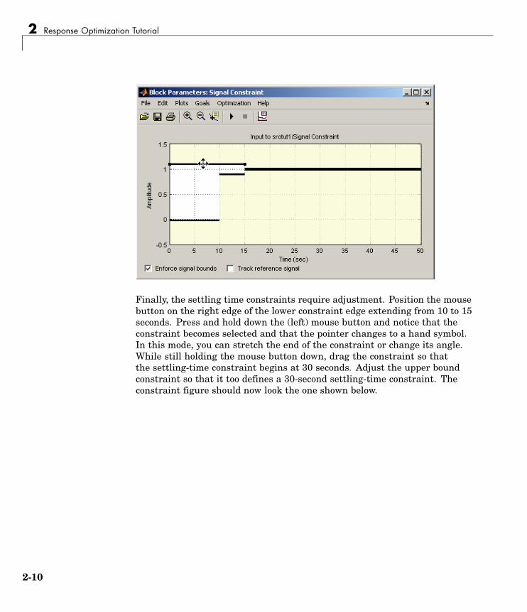
Finally, the settling time constraints require adjustment. Position the mousebutton on the right edge of the lower constraint edge extending from 10 to 15seconds. Press and hold down the (left) mouse button and notice that theconstraint becomes selected and that the pointer changes to a hand symbol.In this mode, you can stretch the end of the constraint or change its angle.While still holding the mouse button down, drag the constraint so thatthe settling-time constraint begins at 30 seconds. Adjust the upper boundconstraint so that it too defines a 30-second settling-time constraint. Theconstraint figure should now look the one shown below.
2-10

Simple Control Design Example
Alternatively, you could set the signal constraints using the Desired Responsedialog box by selecting Goals > Desired Response from the SignalConstraint window. For more information on setting signal constraints, seethe online documentation.
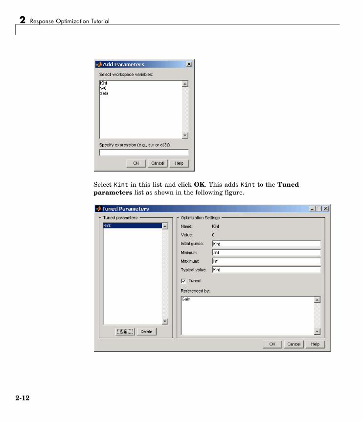
Specifying Tuned ParametersBefore beginning the optimization, you must tell Simulink ResponseOptimization which variables the optimization should tune. Open the TunedParameters dialog box by selecting Optimization > Tuned Parameterswithin the Signal Constraint window. Add the parameter Kint to theTuned parameters list by clicking the Add button. This opens the SelectParameters dialog box with a list of all model parameters that are currentlyin the workspace.
2-11
2 Response Optimization Tutorial
Select Kint in this list and click OK. This adds Kint to the Tunedparameters list as shown in the following figure.
2-12
Simple Control Design Example
To display the optimization settings for this parameter, click Kint in theTuned parameters list. The settings appear under Optimization settingson the right. To constrain Kint to be positive, enter 0 as the Minimum value.For more information on the various tuned parameter settings, see the onlinedocumentation.
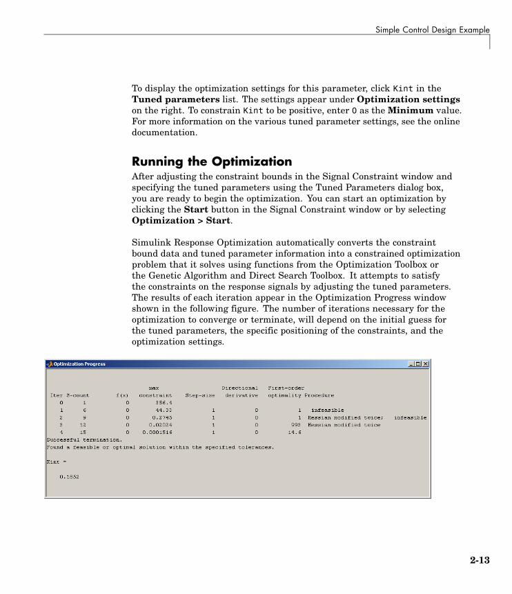
Running the OptimizationAfter adjusting the constraint bounds in the Signal Constraint window andspecifying the tuned parameters using the Tuned Parameters dialog box,you are ready to begin the optimization. You can start an optimization byclicking the Start button in the Signal Constraint window or by selectingOptimization > Start.
Simulink Response Optimization automatically converts the constraintbound data and tuned parameter information into a constrained optimizationproblem that it solves using functions from the Optimization Toolbox orthe Genetic Algorithm and Direct Search Toolbox. It attempts to satisfythe constraints on the response signals by adjusting the tuned parameters.The results of each iteration appear in the Optimization Progress windowshown in the following figure. The number of iterations necessary for theoptimization to converge or terminate, will depend on the initial guess forthe tuned parameters, the specific positioning of the constraints, and theoptimization settings.
2-13

2 Response Optimization Tutorial
In this case the optimization converges after four iterations. For moreinformation about the results shown in the Optimization Progress window,see the online documentation.
The Signal Constraint window, shown in the following figure, plots theresponses at each iteration.
The blue line shows the initial response and the black line shows the current,or final, response. As you can see, the final response signal lies within theconstraint bounds.
The new value of the tuned parameter Kint appears in the OptimizationProgress window and is also changed in the MATLAB workspace. In thiscase the new value of Kint is 0.1852
Because of different numerical precision, the results of the optimization maydiffer slightly across different platforms.
2-14
Simple Control Design Example
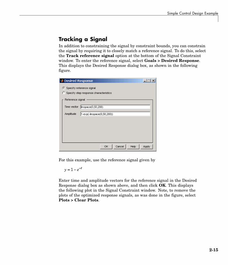
Tracking a SignalIn addition to constraining the signal by constraint bounds, you can constrainthe signal by requiring it to closely match a reference signal. To do this, selectthe Track reference signal option at the bottom of the Signal Constraintwindow. To enter the reference signal, select Goals > Desired Response.This displays the Desired Response dialog box, as shown in the followingfigure.
For this example, use the reference signal given by
Enter time and amplitude vectors for the reference signal in the DesiredResponse dialog box as shown above, and then click OK. This displaysthe following plot in the Signal Constraint window. Note, to remove theplots of the optimized response signals, as was done in the figure, selectPlots > Clear Plots.
2-15

2 Response Optimization Tutorial
Before running the optimization, change the function tolerance to 0.01within the Options dialog box. This ensures that the new objective functionmeets the imposed tolerances. To do this, open the Options dialog box byselecting Optimization > Optimization Options from the menu in theSignal Constraint window and then change the Function tolerance value to0.01 within the Optimization Options pane of the Options dialog box, asshown in the following figure.
2-16
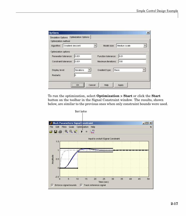
Simple Control Design Example
To run the optimization, select Optimization > Start or click the Startbutton on the toolbar in the Signal Constraint window. The results, shownbelow, are similar to the previous ones when only constraint bounds were used.
2-17

2 Response Optimization Tutorial
The Optimization Progress window shows the final value of Kint.
Before proceeding to the next section, make sure to clear the Track referencesignal check box at the bottom of the Signal Constraint window.
Adding UncertaintyIn your particular problem, you might not have a precise plant model. Insteadyou might know what the nominal plant should be and have some idea ofthe uncertainty inherent in various components of the plant. For example,assume that the plant parameter zeta varies 5% about its nominal valueand w0 varies between 0.7 and 1.45.
When using a Signal Constraint block to optimize response, SimulinkResponse Optimization allows you to optimize response signals in the faceof this uncertainty by specifying uncertainty in parameter values. Note thatyou cannot add uncertainty to parameters or compensator elements whenoptimizing responses in a SISO Design Task.
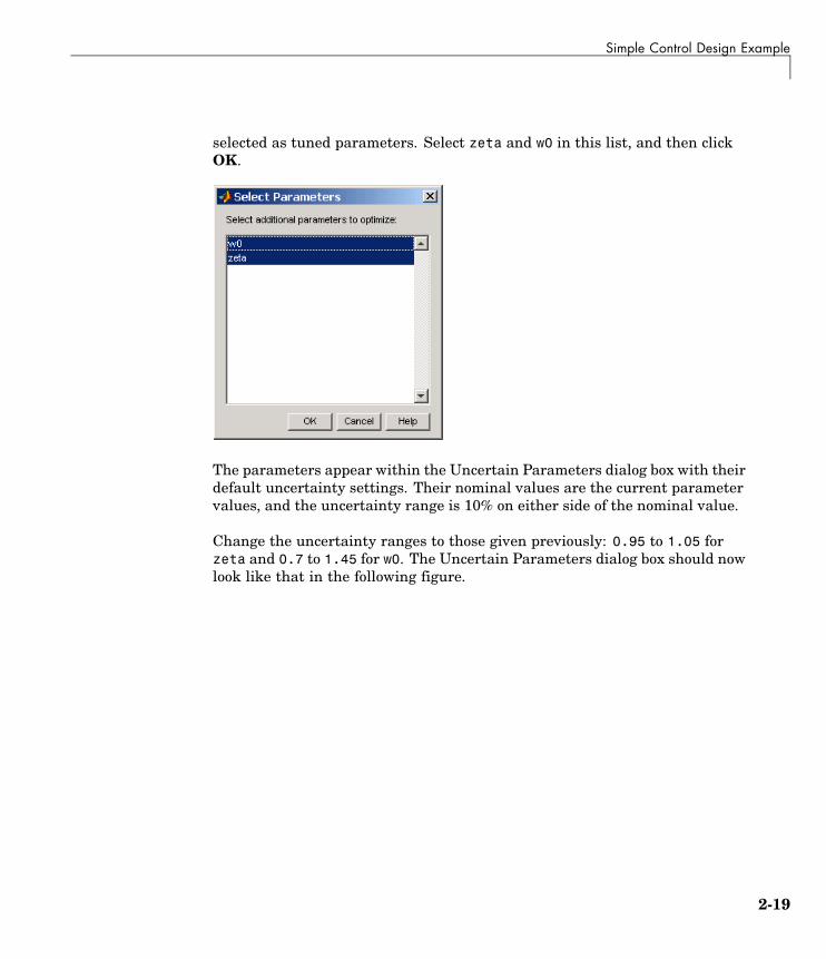
Open the Uncertain Parameters dialog box by selectingOptimization > Uncertain Parameters in the Signal Constraintwindow. To add zeta and w0 as uncertain parameters, click the Add button,which opens the Select Parameters dialog box. This dialog box contains allparameters from the model that are currently in the workspace and are not
2-18
Simple Control Design Example
selected as tuned parameters. Select zeta and w0 in this list, and then clickOK.
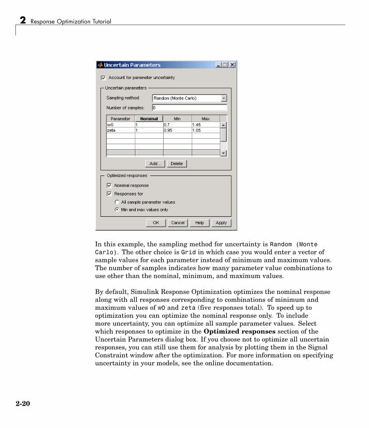
The parameters appear within the Uncertain Parameters dialog box with theirdefault uncertainty settings. Their nominal values are the current parametervalues, and the uncertainty range is 10% on either side of the nominal value.
Change the uncertainty ranges to those given previously: 0.95 to 1.05 forzeta and 0.7 to 1.45 for w0. The Uncertain Parameters dialog box should nowlook like that in the following figure.
2-19
2 Response Optimization Tutorial
In this example, the sampling method for uncertainty is Random (MonteCarlo). The other choice is Grid in which case you would enter a vector ofsample values for each parameter instead of minimum and maximum values.The number of samples indicates how many parameter value combinations touse other than the nominal, minimum, and maximum values.
By default, Simulink Response Optimization optimizes the nominal responsealong with all responses corresponding to combinations of minimum andmaximum values of w0 and zeta (five responses total). To speed up tooptimization you can optimize the nominal response only. To includemore uncertainty, you can optimize all sample parameter values. Selectwhich responses to optimize in the Optimized responses section of theUncertain Parameters dialog box. If you choose not to optimize all uncertainresponses, you can still use them for analysis by plotting them in the SignalConstraint window after the optimization. For more information on specifyinguncertainty in your models, see the online documentation.
2-20
Simple Control Design Example
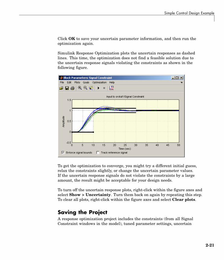
Click OK to save your uncertain parameter information, and then run theoptimization again.
Simulink Response Optimization plots the uncertain responses as dashedlines. This time, the optimization does not find a feasible solution due tothe uncertain response signals violating the constraints as shown in thefollowing figure.
To get the optimization to converge, you might try a different initial guess,relax the constraints slightly, or change the uncertain parameter values.If the uncertain response signals do not violate the constraints by a largeamount, the result might be acceptable for your design needs.
To turn off the uncertain response plots, right-click within the figure axes andselect Show > Uncertainty. Turn them back on again by repeating this step.To clear all plots, right-click within the figure axes and select Clear plots.
Saving the ProjectA response optimization project includes the constraints (from all SignalConstraint windows in the model), tuned parameter settings, uncertain
2-21

2 Response Optimization Tutorial
parameter settings, and settings for the optimization and simulation. Aftercreating a project, you can save it for later use.
To save this project, select File > Save in the Signal Constraint window. Thisopens the Save Project dialog box as shown below.
You can save the project to either a MATLAB workspace variable, modelworkspace variable, or a MAT-file. By selecting the Save and reload projectwith Simulink model check box, the project will automatically reload whenyou reopen the model. If the model cannot find the saved project when youreopen it, it gives a warning.
For more information on saving and reloading projects, see the onlinedocumentation.
2-22
Frequency Domain Response Optimization Example
Frequency Domain Response Optimization ExampleWhen you have the Control System Toolbox, you can place Simulink ResponseOptimization design requirements or constraints on plots in the SISO DesignTool graphical tuning editor and analysis plots that are part of a SISODesign Task. This allows you to include design requirements for responseoptimization in the frequency-domain in addition to the time-domain.
You can specify frequency-domain design requirements to optimize responsesignals for any model that you can design within a SISO Design Task:
• Command-line LTI models created with the Control System Toolbox
• Simulink models that have been linearized using Simulink Control Design
This section guides you through an example using frequency-domain designrequirements to optimize the response of a system in the SISO Design Task.The example uses a linearized version of the srotut1 model from “SimpleControl Design Example” on page 2-6 and uses response optimization todesign a compensator so that the closed loop system meets the followingdesign specifications when you excite the system with a unit step input:
• A maximum 30-second settling time
• A maximum 10% overshoot
• A maximum 10-second rise time
• A limit of ±0.7 on the actuator signal
Creating an LTI Plant ModelIn the srotut1 model, the plant model is composed of a gain, a limitedintegrator, a transfer function, and a transport delay.
You want to design the compensator for the open loop transfer functionof the linearized srotut1 model. The linearized srotut1 plant model iscomposed of the gain, an unlimited integrator, the transfer function, and aPadé approximation to the transport delay.
To create an open loop transfer function based on the linearized srotut1model, enter the following commands:
2-23
2 Response Optimization Tutorial
w0 = 1;zeta = 1;Kint = 0.5;Tdelay = 1;[delayNum,delayDen] = pade(Tdelay,1);integrator = tf(Kint,[1 0]);transfer_fcn = tf(w0^2,[1 2*w0*zeta w0^2]);delay_block = tf(delayNum,delayDen);open_loopTF = integrator*transfer_fcn*delay_block;
Note It is also possible to directly linearize the Simulink model srotut1using the product Simulink Control Design.
Creating Design and Analysis PlotsThis example uses a root locus diagram to design the response of the open looptransfer function, open_loopTF. To create a SISO Design Task, that contains aroot-locus plot, for the open loop transfer function, use the following command:
sisotool('rlocus',open_loopTF)
A SISO Design Task is created within the Control and Estimation ToolsManager, as shown below.
2-24
Frequency Domain Response Optimization Example
The SISO Design Task also contains a root locus diagram in the SISO DesignTool graphical tuning editor.
2-25

2 Response Optimization Tutorial
The Control and Estimation Tools Manager is a graphical environment formanaging and performing tasks such as the design of SISO systems. TheSISO Design Task node contains five panels that perform actions relatedto designing SISO control systems.
The Architecture pane, within the SISO Design Task node, lets you choosethe architecture for the control system you are designing. This example usesthe default architecture. In this system, the plant model, G, is the open looptransfer function open_loopTF, the prefilter, F, and the sensor, H, are set to
2-26

Frequency Domain Response Optimization Example
1, and the compensator, C, is the compensator that will be designed usingresponse optimization methods.
In addition to the root-locus diagram, it is helpful to visualize the response ofthe system with a step response plot. To add a step response:
1 Select the Analysis Plots pane with the SISO Design Task node of theControl and Estimation Tool Manager.
2 Select Step for the Plot Type of Plot 1.
3 Under Contents of Plots, select the check box in column 1 for the responseClosed Loop r to y.
A step response plot appears in an LTI Viewer. The plot shows the responseof the closed loop system from r (input to the prefilter, F) to y (output of theplant model, G):
2-27
2 Response Optimization Tutorial
Creating a Response Optimization TaskThere are several possible methods for designing a SISO system; this exampleuses an automated approach involving response optimization methods. Aftercreating the design and analysis plots in “Creating Design and Analysis Plots”on page 2-24, you are ready to start a response optimization task to designthe compensator.
To create a Simulink Response Optimization task:
1 Select the Automated Tuning pane within the SISO Design Task nodein the Control and Estimation Tools Manager.
2-28

Frequency Domain Response Optimization Example
2 In the Analysis Plots pane, select Optimization based tuning as theDesign Method.
3 Click the Optimize Compensators button to create the ResponseOptimization node under the SISO Design Task node in the tree browserin the left pane of the Control and Estimation Tools Manager.
The Response Optimization node contains four panes. With the exception ofthe first pane, each corresponds to a step in the response optimization process:
• Overview: A schematic diagram of the response optimization process.
• Compensators: Select and configure the compensator elements that youwant to tune. See “Selecting Tunable Compensator Elements” on page 2-29.
• Design requirements: Select the design requirements that you wantthe system to meet after tuning the compensator elements. See “AddingDesign Requirements” on page 2-30.
• Optimization: Configure optimization options and view the progress ofthe response optimization. See “Optimizing the System’s Response” onpage 2-39.
Note When optimizing responses in a SISO Design Task, you cannot adduncertainty to parameters or compensator elements.
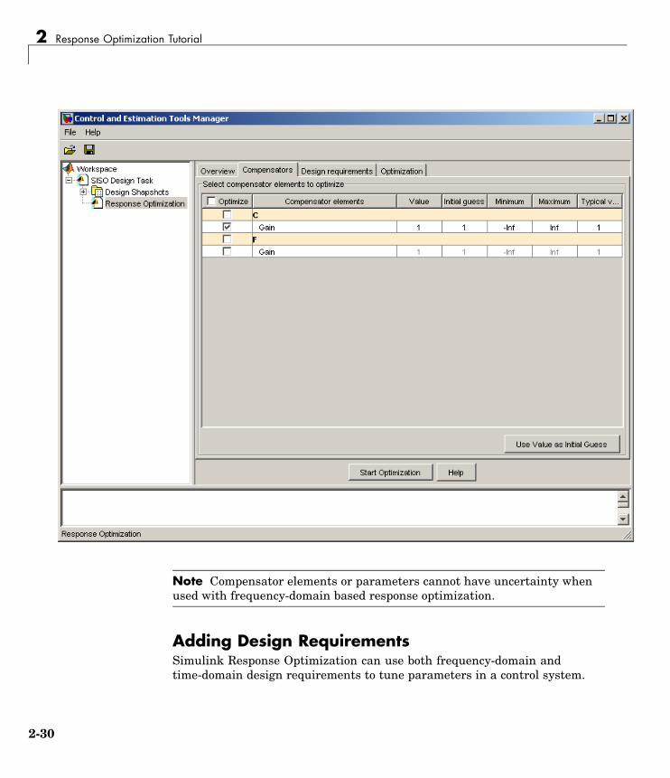
Selecting Tunable Compensator ElementsSimulink Response Optimization tunes elements or parameters withincompensators in your system so that the response of the system meets thedesign requirements you specify. To specify the compensator elements to tune:
1 Select the Compensators pane within the Response Optimization node.
2 Within the Compensators pane, select the check boxes in the Optimizecolumn that correspond to the compensator elements you want to tune.
In this example, to tune the Gain in the compensator C, select the checkbox next to this element, as shown below.
2-29
2 Response Optimization Tutorial
Note Compensator elements or parameters cannot have uncertainty whenused with frequency-domain based response optimization.
Adding Design RequirementsSimulink Response Optimization can use both frequency-domain andtime-domain design requirements to tune parameters in a control system.
2-30
Frequency Domain Response Optimization Example
The Design requirements pane within the Response Optimization nodeof the Control and Estimation Tools Manager provides an interface to createnew design requirements and select those you want to use for a responseoptimization.
This example uses the design specifications from “Frequency DomainResponse Optimization Example” on page 2-23. The following sections eachcreate a new design requirement to meet these specifications.
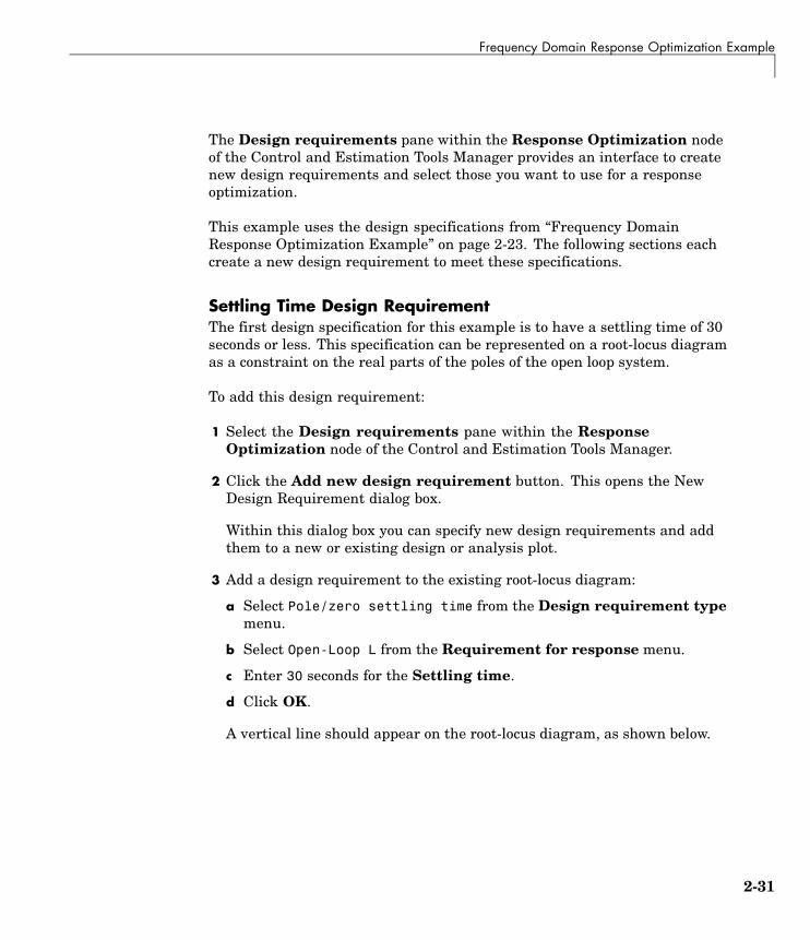
Settling Time Design RequirementThe first design specification for this example is to have a settling time of 30seconds or less. This specification can be represented on a root-locus diagramas a constraint on the real parts of the poles of the open loop system.
To add this design requirement:
1 Select the Design requirements pane within the ResponseOptimization node of the Control and Estimation Tools Manager.
2 Click the Add new design requirement button. This opens the NewDesign Requirement dialog box.
Within this dialog box you can specify new design requirements and addthem to a new or existing design or analysis plot.
3 Add a design requirement to the existing root-locus diagram:
a Select Pole/zero settling time from the Design requirement typemenu.
b Select Open-Loop L from the Requirement for response menu.
c Enter 30 seconds for the Settling time.
d Click OK.
A vertical line should appear on the root-locus diagram, as shown below.
2-31

2 Response Optimization Tutorial
Overshoot Design RequirementThe second design specification for this example is to have a percentageovershoot of 10% or less. This specification is related to the damping ratio ona root-locus diagram. In addition to adding a design requirement with theAdd new design requirement button, you can also right-click directly onthe design or analysis plots to add the requirement, as shown below.
To add this design requirement:
2-32

Frequency Domain Response Optimization Example
1 Right-click anywhere within the white space of the root-locus diagram inthe SISO Design Tool window. Select Design Requirements > New toopen the New Design Requirement dialog box.
2 Select Percent overshoot as the Design requirement type and enter 10as the Percent overshoot.
3 Click OK to add the design requirement to the root-locus diagram. Thedesign requirement appears as two lines radiating at an angle from theorigin, as shown below.
2-33
2 Response Optimization Tutorial
Rise Time Design RequirementThe third design specification for this example is to have a rise time of10 seconds or less. This specification is related to a lower limit on a BodeMagnitude diagram.
To add this design requirement:
1 Select the Graphical Tuning pane within the SISO Design Task node ofthe Control and Estimation Tools Manager.
2 For Plot 2, set Plot Type to Open-Loot Bode.
3 Right-click anywhere within the white space of the root-locus diagram inthe SISO Design Tool window. Select Design Requirements > New toopen the New Design Requirement dialog box.
4 Create a design requirement representing the rise time and add it to anew Bode plot:
a Select Lower gain limit from the Design requirement type menu.
b Enter 1e-2 to 0.17 for the Frequency range.
c Enter 0 to 0 for the Magnitude range.
d Click OK.
A Bode diagram appears within the SISO Design Tool window. Themagnitude plot of the Bode diagram includes a horizontal line representingthe design requirement, as shown below.
2-34
Frequency Domain Response Optimization Example
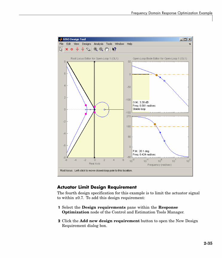
Actuator Limit Design RequirementThe fourth design specification for this example is to limit the actuator signalto within ±0.7. To add this design requirement:
1 Select the Design requirements pane within the ResponseOptimization node of the Control and Estimation Tools Manager.
2 Click the Add new design requirement button to open the New DesignRequirement dialog box.
2-35
2 Response Optimization Tutorial
3 Create a time-domain design requirement representing the upper limit onthe actuator signal, and add it to a new step response plot in the LTI Viewer:
a Select Step response upper amplitude limit from the Designrequirement type menu.
b Select Closed Loop r to u from the Requirement for responsemenu.
c Enter 0 to 10 for the Time range.
d Enter 0.7 to 0.7 for the Amplitude range.
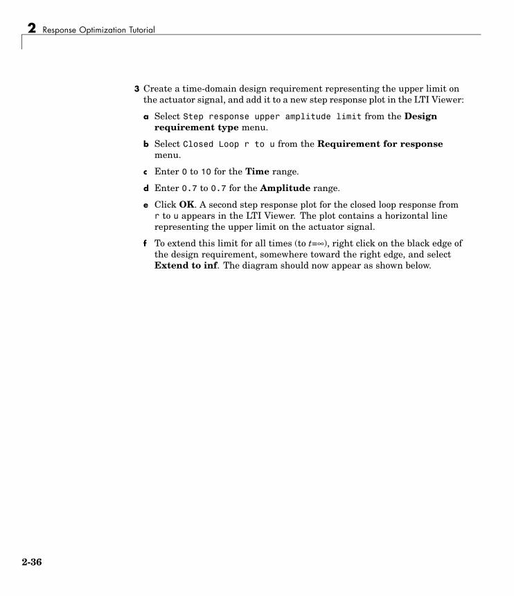
e Click OK. A second step response plot for the closed loop response fromr to u appears in the LTI Viewer. The plot contains a horizontal linerepresenting the upper limit on the actuator signal.
f To extend this limit for all times (to t=∞), right click on the black edge ofthe design requirement, somewhere toward the right edge, and selectExtend to inf. The diagram should now appear as shown below.
2-36
Frequency Domain Response Optimization Example
To add the corresponding design requirement for the lower limit on theactuator signal:
1 Within the white space of the lower step response plot, right-click and selectDesign Requirements > New to open the New Design Requirementdialog box.
2 Create a time-domain design requirement representing the lower limit onthe actuator signal, and add it to the step response plot in the LTI Viewer:
a Select Step response lower amplitude limit from the Designrequirement type menu.
b Select Closed Loop r to u from the Requirement for responsemenu.
2-37

2 Response Optimization Tutorial
c Enter 0 to 10 for the Time range.
d Enter -0.7 to -0.7 for the Amplitude range.
e Click OK. The step response plot now contains a second horizontal linerepresenting the lower limit on the actuator signal.
f To extend this limit for all times (to t=∞), right-click in the yellow shadedarea and select Extend to inf. The diagram should now appear asshown below.
Selecting the Design Requirements to Use During ResponseOptimizationThe design requirements give constraints on the dynamics of the systemand the values of response signals. The table lists all design requirements
2-38

Frequency Domain Response Optimization Example
in the design and analysis plots. Select the check boxes next to the designrequirements you want to use in the response optimization. This exampleuses all the current design requirements.
Optimizing the System’s ResponseAfter selecting the compensator elements to tune and adding designrequirements for the response signals to satisfy, you are ready to being theresponse optimization.
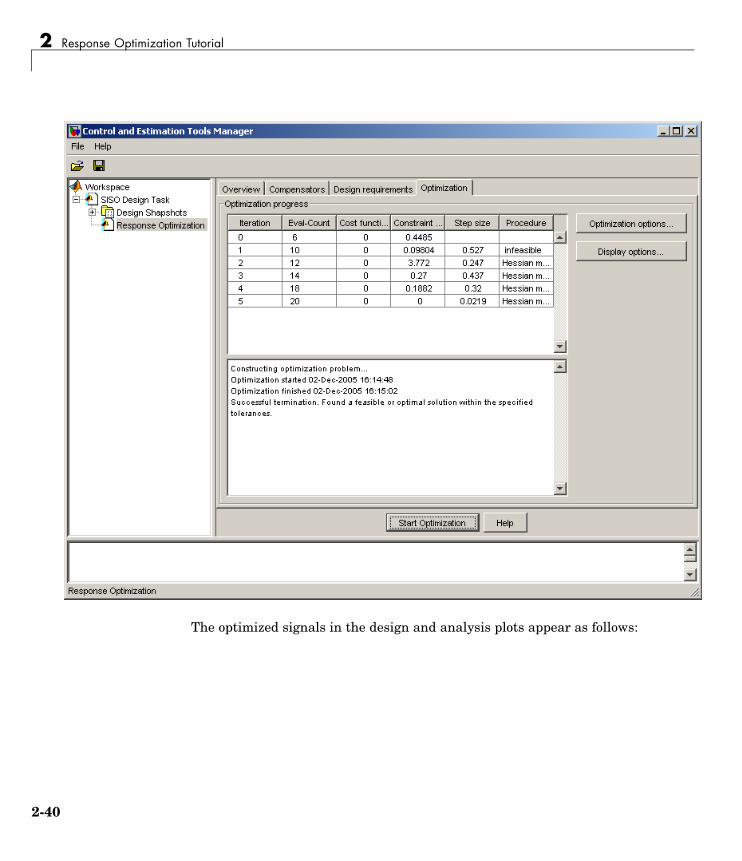
The Optimization pane within the Response Optimization node of theControl and Estimation Tools Manager displays the progress of the responseoptimization. The pane also contains options to configure the types of progressinformation displayed during the optimization and options to configure theoptimization methods and algorithms.
To optimize the response of the system in this example, click the StartOptimization button.
The Optimization pane displays the progress of the optimization, iterationby iteration, as shown below. Termination messages from the optimizationalgorithm and suggestions for improving convergence also appear here.
2-39
2 Response Optimization Tutorial
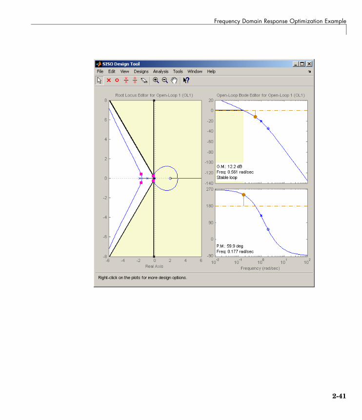
The optimized signals in the design and analysis plots appear as follows:
2-40
Frequency Domain Response Optimization Example
2-41

2 Response Optimization Tutorial
Creating and Displaying the Closed-Loop SystemAfter designing a compensator by optimizing the response of the system, youcan create export the compensator to the MATLAB Workspace and create amodel of the full closed-loop system.
1 Within the SISO Design Tool window, select File > Export to open theSISO Tool Export dialog box.
2 Select the compensator you designed, Compensator C, and then clickthe Export to Workspace button.
2-42

Frequency Domain Response Optimization Example
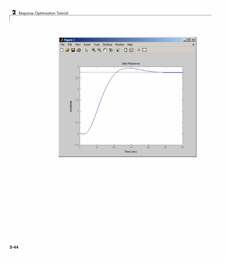
At the command line, enter the following command to create the closed-loopsystem, CL, from the open-loop transfer function, open_loopTF, and thecompensator, C:
CL=feedback(open_loopTF,C);
This returns the following model:
Zero/pole/gain:-0.5 (s-2)
-------------------------------------------------(s^2 + 0.4244s + 0.1079) (s^2 + 3.576s + 3.375)
To create a step response plot of the closed loop system, enter the followingcommand:
step(CL);
This produces the following figure:
2-43
2 Response Optimization Tutorial
2-44
Physical Modeling Example
Physical Modeling ExampleThe following example demonstrates further techniques for using SimulinkResponse Optimization to directly tune Simulink models. It uses the modelsrotut2 to show how to constrain more than one signal and tune multipleparameters.
Specifically, you will design a hydraulic system that extends a piston by 0.07m while keeping the pressure from the pump below 12x105 Pa. The physicalsystem consists of a hydraulic pump supplying pressure to a hydrauliccylinder. The cylinder contains a piston, which extends and compressesa spring. This system is modeled in the Simulink model srotut2. Thesystem parameters that you can adjust, or tune, to achieve the requireddesign characteristics are the cross-sectional area of the piston, Ac, and themaximum pump flow-rate, Qmax.
The specifications for the response of the piston position signal are
• Maximum overshoot of 15%
• Rise time of 0.25 second
• Settle to within 10% of final value after 0.5 second
• Final value of 0.07 m
The specifications for the response of the pump pressure signal are
• Lower bound of zero (Pressures below this value are not physically possible.)
• Upper bound of 12x105 Pa
Opening the Hydraulic Cylinder ModelThe Simulink system srotut2 contains a block diagram representation ofthe hydraulic system described above. You can open the system by typingsrotut2 at the MATLAB prompt.
2-45

2 Response Optimization Tutorial
Notice that the system contains two Signal Constraint blocks. These blocksdefine constraints on the piston position and pump pressure signals. SimulinkResponse Optimization allows you to constrain multiple responses includingresponses within subsystems of your model. For each signal that you want toconstrain, you need to attach a Signal Constraint block. Within each SignalConstraint block, set constraint bounds and/or reference signals for eachsignal. The tuned and uncertain parameters, along with optimization andsimulation options are set for the whole system within any one of the SignalConstraint blocks.
2-46
Physical Modeling Example
Adjusting ConstraintsIn this section you will adjust the signal constraints in the system.
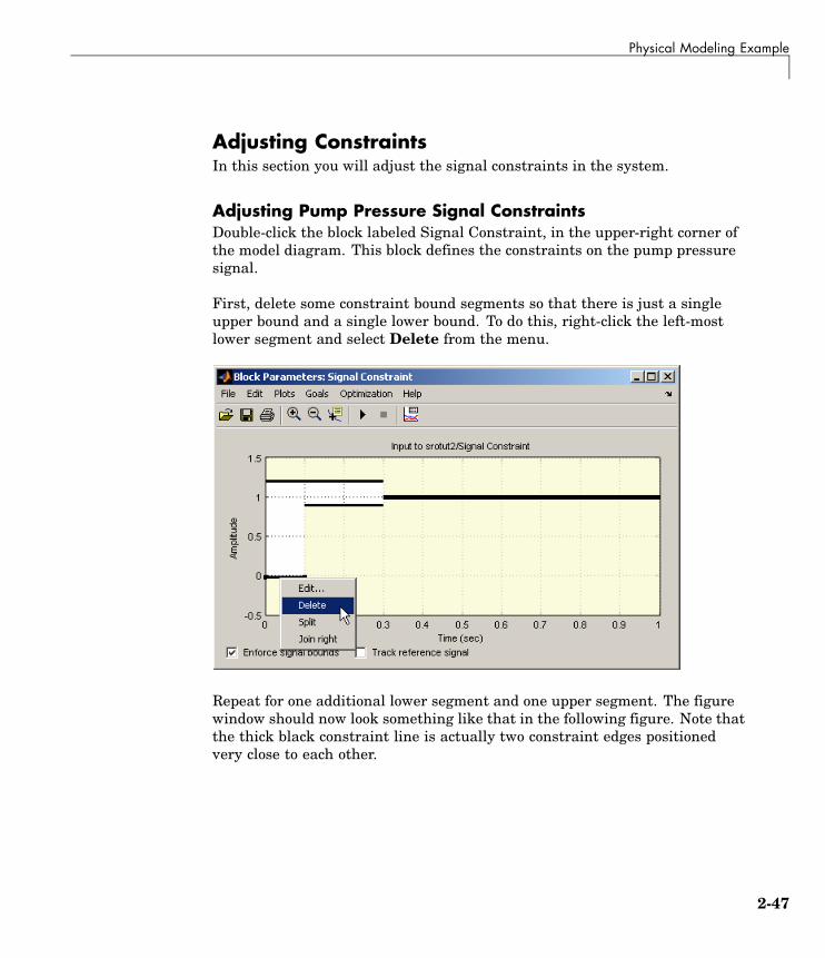
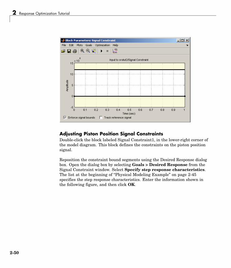
Adjusting Pump Pressure Signal ConstraintsDouble-click the block labeled Signal Constraint, in the upper-right corner ofthe model diagram. This block defines the constraints on the pump pressuresignal.
First, delete some constraint bound segments so that there is just a singleupper bound and a single lower bound. To do this, right-click the left-mostlower segment and select Delete from the menu.
Repeat for one additional lower segment and one upper segment. The figurewindow should now look something like that in the following figure. Note thatthe thick black constraint line is actually two constraint edges positionedvery close to each other.
2-47
2 Response Optimization Tutorial
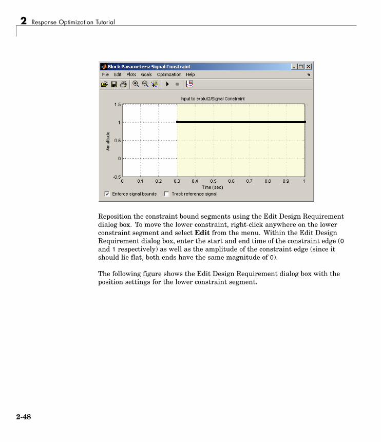
Reposition the constraint bound segments using the Edit Design Requirementdialog box. To move the lower constraint, right-click anywhere on the lowerconstraint segment and select Edit from the menu. Within the Edit DesignRequirement dialog box, enter the start and end time of the constraint edge (0and 1 respectively) as well as the amplitude of the constraint edge (since itshould lie flat, both ends have the same magnitude of 0).
The following figure shows the Edit Design Requirement dialog box with theposition settings for the lower constraint segment.
2-48
Physical Modeling Example
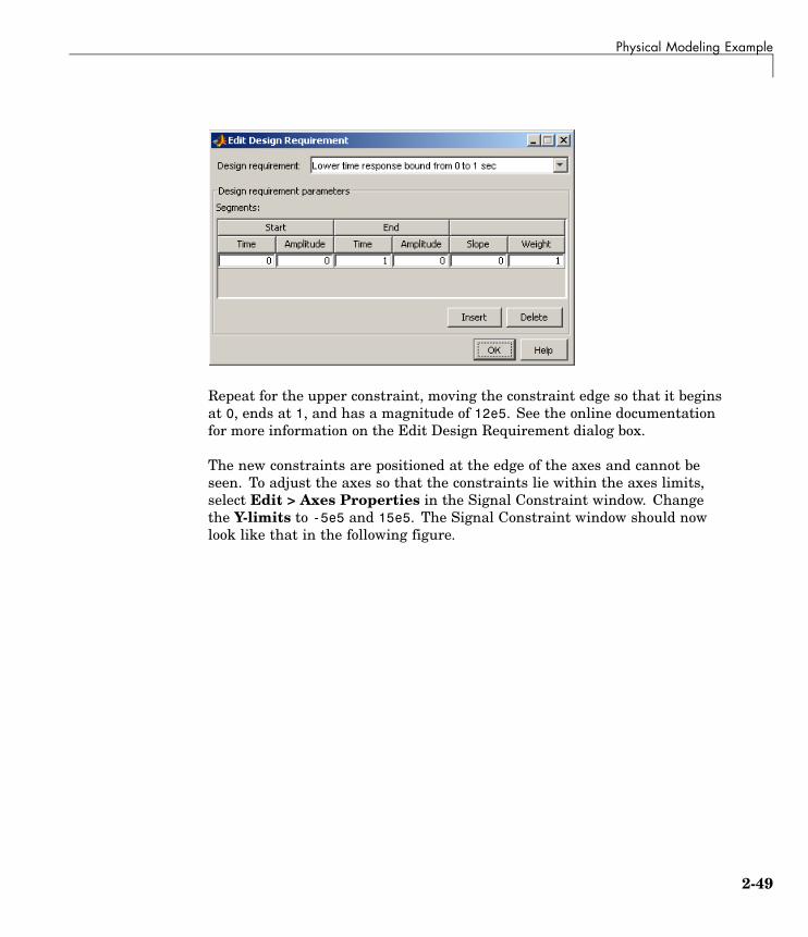
Repeat for the upper constraint, moving the constraint edge so that it beginsat 0, ends at 1, and has a magnitude of 12e5. See the online documentationfor more information on the Edit Design Requirement dialog box.
The new constraints are positioned at the edge of the axes and cannot beseen. To adjust the axes so that the constraints lie within the axes limits,select Edit > Axes Properties in the Signal Constraint window. Changethe Y-limits to -5e5 and 15e5. The Signal Constraint window should nowlook like that in the following figure.
2-49
2 Response Optimization Tutorial
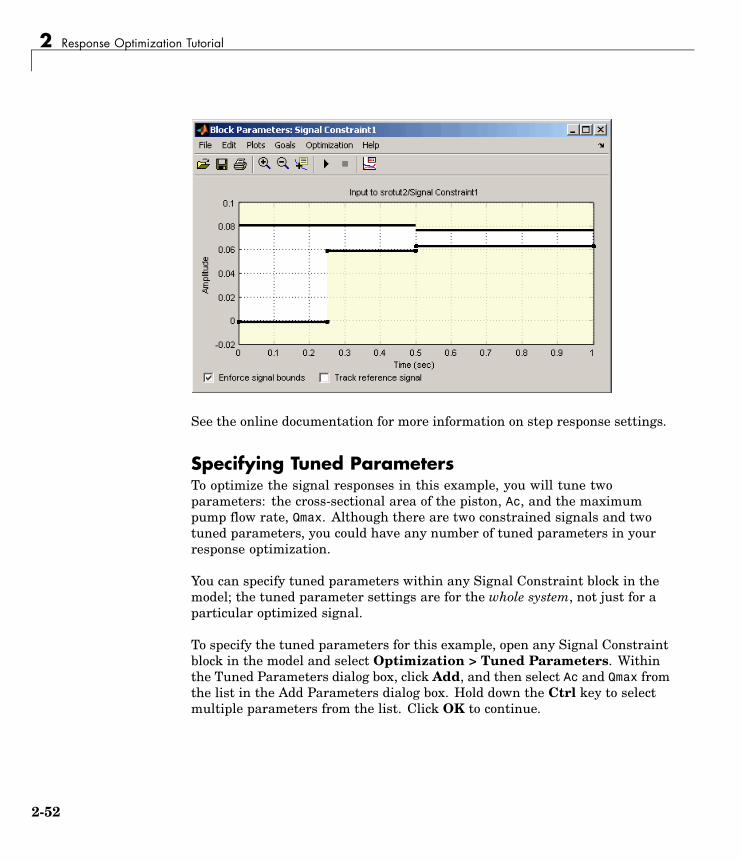
Adjusting Piston Position Signal ConstraintsDouble-click the block labeled Signal Constraint1, in the lower-right corner ofthe model diagram. This block defines the constraints on the piston positionsignal.
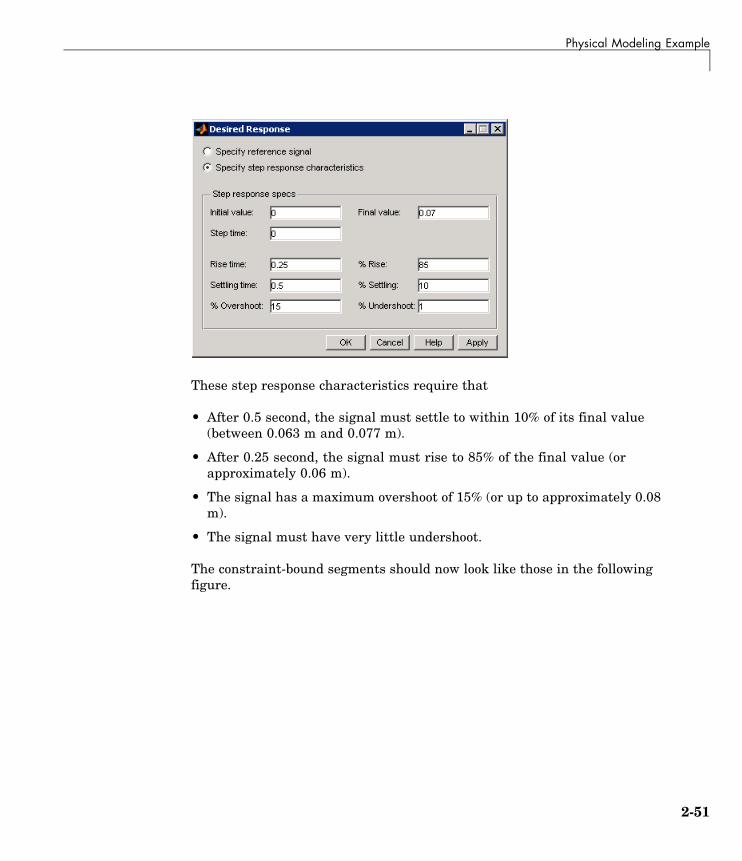
Reposition the constraint bound segments using the Desired Response dialogbox. Open the dialog box by selecting Goals > Desired Response from theSignal Constraint window. Select Specify step response characteristics.The list at the beginning of “Physical Modeling Example” on page 2-45specifies the step response characteristics. Enter the information shown inthe following figure, and then click OK.
2-50
Physical Modeling Example
These step response characteristics require that
• After 0.5 second, the signal must settle to within 10% of its final value(between 0.063 m and 0.077 m).
• After 0.25 second, the signal must rise to 85% of the final value (orapproximately 0.06 m).
• The signal has a maximum overshoot of 15% (or up to approximately 0.08m).
• The signal must have very little undershoot.
The constraint-bound segments should now look like those in the followingfigure.
2-51
2 Response Optimization Tutorial
See the online documentation for more information on step response settings.
Specifying Tuned ParametersTo optimize the signal responses in this example, you will tune twoparameters: the cross-sectional area of the piston, Ac, and the maximumpump flow rate, Qmax. Although there are two constrained signals and twotuned parameters, you could have any number of tuned parameters in yourresponse optimization.
You can specify tuned parameters within any Signal Constraint block in themodel; the tuned parameter settings are for the whole system, not just for aparticular optimized signal.
To specify the tuned parameters for this example, open any Signal Constraintblock in the model and select Optimization > Tuned Parameters. Withinthe Tuned Parameters dialog box, click Add, and then select Ac and Qmax fromthe list in the Add Parameters dialog box. Hold down the Ctrl key to selectmultiple parameters from the list. Click OK to continue.
2-52

Physical Modeling Example
In the Tuned Parameters dialog box, enter specifications for each tunedparameter by selecting the parameter in the list on the left, and then enteringinformation such as initial guesses, minimum values, and maximum valueson the right. For Ac, enter 0 as a Minimum value since it does not makesense for the cross-sectional area to be negative. Similarly, enter 0 as aMinimum value for Qmax to avoid negative flow rates, which imply that theflow reverses direction through the system.
See the online documentation for more information on tuned parametersettings.
Running the OptimizationAfter adjusting the constraints and defining tuned parameters, start theoptimization by selecting Optimization > Start, or by clicking the Startbutton below the menu bar in a Signal Constraint window.
In this case the optimization algorithm is not able to find a solution thatsatisfies all the constraints, as seen in the Optimization Progress windowbelow.
2-53
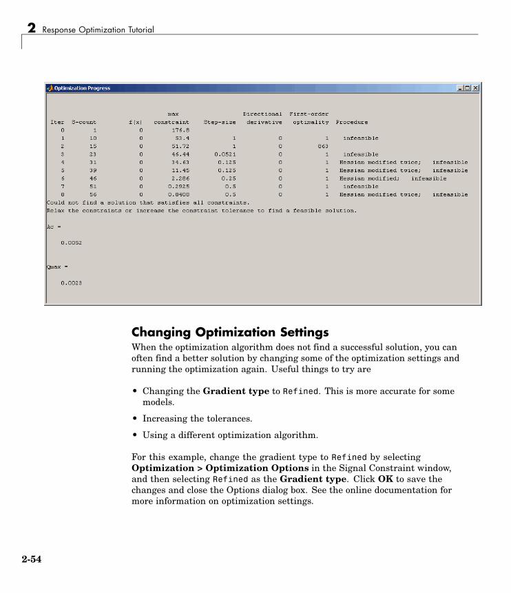
2 Response Optimization Tutorial
Changing Optimization SettingsWhen the optimization algorithm does not find a successful solution, you canoften find a better solution by changing some of the optimization settings andrunning the optimization again. Useful things to try are
• Changing the Gradient type to Refined. This is more accurate for somemodels.
• Increasing the tolerances.
• Using a different optimization algorithm.
For this example, change the gradient type to Refined by selectingOptimization > Optimization Options in the Signal Constraint window,and then selecting Refined as the Gradient type. Click OK to save thechanges and close the Options dialog box. See the online documentation formore information on optimization settings.
2-54
Physical Modeling Example
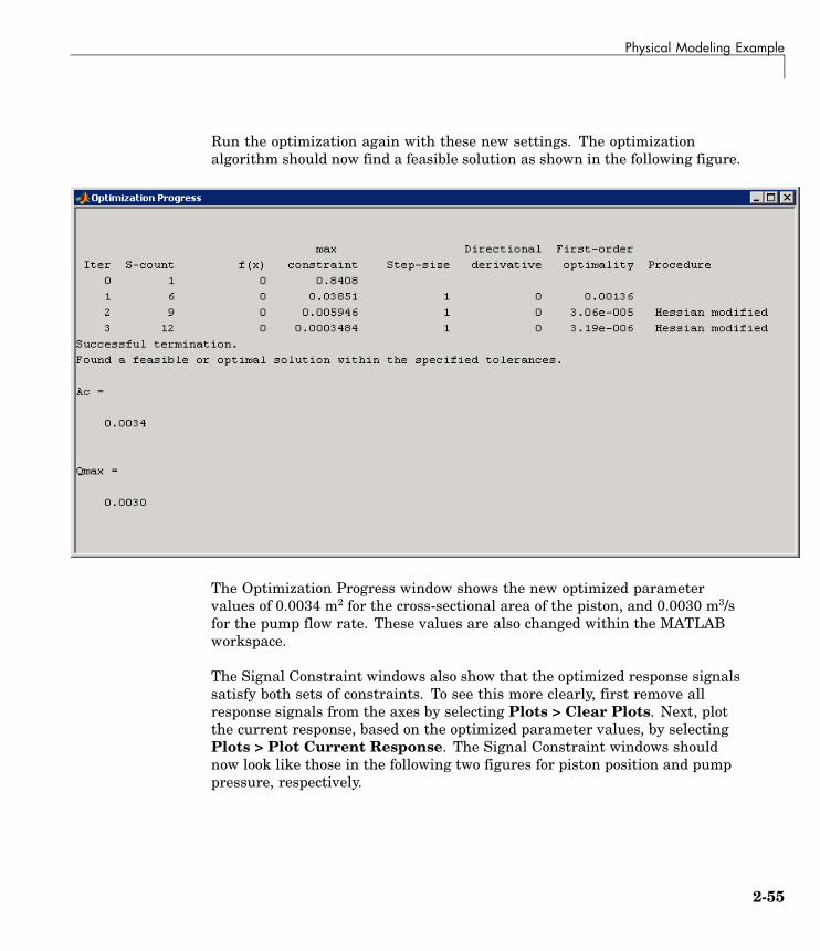
Run the optimization again with these new settings. The optimizationalgorithm should now find a feasible solution as shown in the following figure.
The Optimization Progress window shows the new optimized parametervalues of 0.0034 m2 for the cross-sectional area of the piston, and 0.0030 m3/sfor the pump flow rate. These values are also changed within the MATLABworkspace.
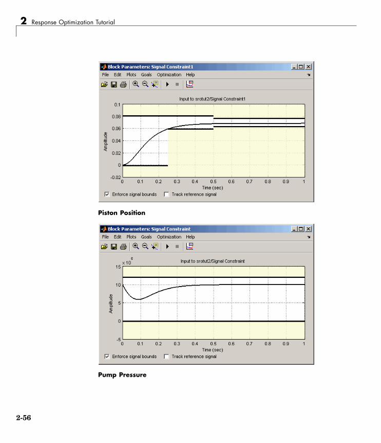
The Signal Constraint windows also show that the optimized response signalssatisfy both sets of constraints. To see this more clearly, first remove allresponse signals from the axes by selecting Plots > Clear Plots. Next, plotthe current response, based on the optimized parameter values, by selectingPlots > Plot Current Response. The Signal Constraint windows shouldnow look like those in the following two figures for piston position and pumppressure, respectively.
2-55
2 Response Optimization Tutorial
Piston Position
Pump Pressure
2-56

Physical Modeling Example
See Chapter 4, “Troubleshooting” for more advice on adjusting the responseoptimization to achieve the desired results.
Finding a Maximally Feasible SolutionAlthough the results in the previous section satisfy the constraints, theresponse signal for the piston position lies near the lower edge of theconstraint region. This is because the optimization stops as soon as a feasiblesolution is found. To search for a solution that satisfies the constraints evenbetter, you can
1 Select Optimization > Optimization Options from a Signal Constraintwindow to open the Options dialog box.
2 Select Look for maximally feasible solution. By selecting this option,Simulink Response Optimization will continue to search for an optimalsolution, after the initial solution is found.
3 Click OK to save the settings and close the Options dialog box.
4 Click the Start button to run the optimization again.
The optimization finds a new solution that lies further inside the constraintregion. The new optimized parameter values are 0.0032 m2 for thecross-sectional area of the piston, and 0.0033 m3/s for the pump flow rate.
2-57

2 Response Optimization Tutorial
2-58
3
Response OptimizationUsing Functions
In addition to the graphical user interface, Simulink Response Optimizationhas a command-line interface that lets you use functions to optimizethe responses of signals within a Simulink model. The command-lineinterface only includes time-domain constraints, not frequency-domainrequirements although it is possible to include parameter uncertainty with thecommand-line interface. This chapter includes an example outlining the use ofthese functions. A function reference is provided in the online documentation.
Control Design Example UsingFunctions (p. 3-2)
An example outlining the responseoptimization process using functions
3 Response Optimization Using Functions
Control Design Example Using FunctionsThis example uses functions to optimize the response of a signal in theSimulink model srotut1. For a more detailed description of these functions,refer to the Function Reference in the online documentation.
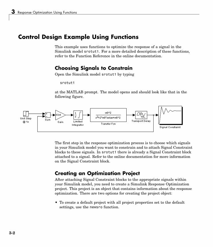
Choosing Signals to ConstrainOpen the Simulink model srotut1 by typing
srotut1
at the MATLAB prompt. The model opens and should look like that in thefollowing figure.
The first step in the response optimization process is to choose which signalsin your Simulink model you want to constrain and to attach Signal Constraintblocks to these signals. In srotut1 there is already a Signal Constraint blockattached to a signal. Refer to the online documentation for more informationon the Signal Constraint block.
Creating an Optimization ProjectAfter attaching Signal Constraint blocks to the appropriate signals withinyour Simulink model, you need to create a Simulink Response Optimizationproject. This project is an object that contains information about the responseoptimization. There are two options for creating the project object:
• To create a default project with all project properties set to the defaultsettings, use the newsro function.
3-2

Control Design Example Using Functions
• To create a project based on the current response optimization settings inthe model, use the getsro function.
Creating a Default ProjectCreate a new project with default settings using the following command:
proj=newsro('srotut1',{'Kint'})
The first input to the newsro function is the model name. The second inputis a cell array of the tuned parameters. In this case Kint is the only tunedparameter.
This returns the following object:
Name: 'srotut1'Parameters: [1x1 ResponseOptimizer.Parameter]
OptimOptions: [1x1 ResponseOptimizer.OptimOptions]Tests: [1x1 ResponseOptimizer.SimTest]Model: 'srotut1'
Simulink Response Optimization Project.
Creating a Project Based on Current Response OptimizationSettingsCreate a new project based on the current response optimization settings inthe model using the following command. This is useful when you previouslysaved a project for the model and want to optimize this project at the commandline or when you have set the project up with the graphical interface andwould like to continue the analysis at the command line.
proj2=getsro('srotut1')
This command returns a project object with the same properties as the objectreturned with newsro, although these properties will possibly have differentcurrent values. The model must already be open to use the getsro function.
3-3
3 Response Optimization Using Functions
Properties of a Response Optimization ProjectWithin the project object you can set characteristics of the tuned parameters,specify uncertain parameters, position constraint bound segments, and setoptions for the optimization and simulations.
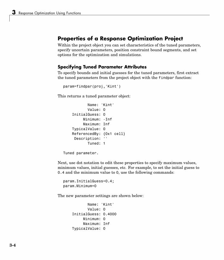
Specifying Tuned Parameter AttributesTo specify bounds and initial guesses for the tuned parameters, first extractthe tuned parameters from the project object with the findpar function:
param=findpar(proj,'Kint')
This returns a tuned parameter object:
Name: 'Kint'Value: 0
InitialGuess: 0Minimum: -InfMaximum: Inf
TypicalValue: 0ReferencedBy: {0x1 cell}Description: ''
Tuned: 1
Tuned parameter.
Next, use dot notation to edit these properties to specify maximum values,minimum values, initial guesses, etc. For example, to set the initial guess to0.4 and the minimum value to 0, use the following commands:
param.InitialGuess=0.4;param.Minimum=0
The new parameter settings are shown below:
Name: 'Kint'Value: 0
InitialGuess: 0.4000Minimum: 0Maximum: Inf
TypicalValue: 0
3-4

Control Design Example Using Functions
ReferencedBy: {0x1 cell}Description: ''
Tuned: 1
Tuned parameter.
For more information on specifying tuned parameters, see the onlinedocumentation.
Adjusting Signal ConstraintsTo define the constrain bound segments within which the optimized signalresponse must lie, first extract a signal constraint object from the project,using the findconstr function:
constr=findconstr(proj,'srotut1/Signal Constraint')
This function takes the project object and the location of a Signal Constraintblock in the model as inputs and creates the following signal constraint object:
ConstrEnable: 'on'isFeasible: 1CostEnable: 'off'
Enable: 'on'Name: 'Signal Constraint'
SignalSize: [1 1]LowerBoundX: [3x2 double]LowerBoundY: [3x2 double]
LowerBoundWeight: [3x1 double]UpperBoundX: [2x2 double]UpperBoundY: [2x2 double]
UpperBoundWeight: [2x1 double]ReferenceX: []ReferenceY: []
ReferenceWeight: []
Signal Constraint.
3-5

3 Response Optimization Using Functions
To move the constraints, edit the LowerBoundX, LowerBoundY, UpperBoundX,and UpperBoundY matrices. These matrices specify the x and y positions of theendpoints of each segment. For example:
To move the constraint bounds to the positions shown in the following figure,use the following commands:
constr.LowerBoundX=[0 12;12 30;30 50];constr.LowerBoundY=[0 0;0.9 0.9;0.99 0.99];constr.UpperBoundX=[0 30;30 50];constr.UpperBoundY=[1.1 1.1;1.01 1.01];
3-6
Control Design Example Using Functions
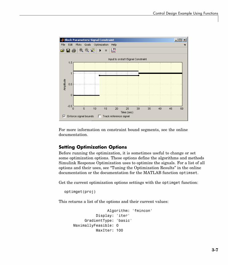
For more information on constraint bound segments, see the onlinedocumentation.
Setting Optimization OptionsBefore running the optimization, it is sometimes useful to change or setsome optimization options. These options define the algorithms and methodsSimulink Response Optimization uses to optimize the signals. For a list of alloptions and their uses, see “Tuning the Optimization Results” in the onlinedocumentation or the documentation for the MATLAB function optimset.
Get the current optimization options settings with the optimget function:
optimget(proj)
This returns a list of the options and their current values:
Algorithm: 'fmincon'Display: 'iter'
GradientType: 'basic'MaximallyFeasible: 0
MaxIter: 100
3-7

3 Response Optimization Using Functions
TolCon: 1.0000e-003TolFun: 1.0000e-003
TolX: 1.0000e-003Restarts: 0
SearchMethod: []
Use the optimset function to change any values within the optimizationoptions object. For example, to change the tolerance on the parameter values,TolX, to 1e-4 use the following command:
optimset(proj,'TolX',1e-4)
Setting Simulation OptionsIn addition to specifying optimization options, it is sometimes useful to specifysimulation options. These options define the solvers, simulation times, andother settings that Simulink Response Optimization uses when simulatingthe models during the response optimization. For a list of all options and theiruses, see “Setting Options for the Simulation” in the online documentation orthe documentation for the Simulink function simset.
Get the current simulation options settings with the simget function:
simget(proj)
This returns a list of the options and their current values:
AbsTol: 1.0000e-006FixedStep: 'auto'
InitialStep: 'auto'MaxStep: 'auto'MinStep: 'auto'RelTol: 1.0000e-003Solver: 'ode45'
ZeroCross: 'on'StartTime: '0.0'StopTime: '50'
To change values within the simulation options object, use the simsetfunction. For example, change the solver to ode23 with the followingcommand:
3-8

Control Design Example Using Functions
simset(proj,'Solver','ode23')
Specifying Uncertain ParametersWhen some parameters in your model are not known exactly, but you do knowthe nominal plant and the level of uncertainty surrounding this model, youcan include this uncertainty in your response optimization by specifyinguncertain parameters in your model.
In this example, assume that w0 varies between 0.8 and 1.2 while zeta variesbetween 0.95 and 1.05. First, create a set of sample parameter values withinthese ranges using the randunc function:
unc_rand=randunc(2,'w0',{0.8 1.2},'zeta',{0.95 1.05});
The randunc function creates combinations of parameter values based on theendpoints of their uncertainty ranges. In addition, it creates several randomparameter value combinations. The first argument to the function specifiesthe number of random parameter value combinations that the functioncreates. The remaining input arguments specify the uncertain parametersand the ranges over which they vary. This particular example creates tworandom combinations of w0 and zeta values in addition to the combinations ofparameter values at the endpoints.
When you would rather specify uncertain parameter values on a grid, usethe gridunc function:
unc_grid=gridunc('w0',{0.8 0.9 1.0 1.1 1.2},'zeta',{0.95 1 1.05});
The gridunc function creates combinations of the given parameters at valuesspecified in the cell-arrays of parameter values.
For more information on creating sets of uncertain parameter valuecombinations, see the reference pages for randunc and gridunc.
By default, when adjusting the tuned parameters, the response optimizationalgorithm does not take responses based on these uncertain parametervalues into account. To include an uncertain parameter combination in theoptimization, you must set its Optimized property to true.
3-9
3 Response Optimization Using Functions
For example, to include all the parameter combinations within unc_rand,enter the following command:
unc_rand.Optimized(1:end)=true
After creating the set of uncertain parameter values, and choosing to includesome or all of them in the optimization, add these values to the project objectwith the setunc function:
setunc(proj,unc_rand)
For more information on specifying uncertain parameter values, see theonline documentation.
Running the OptimizationTo run the optimization for this project, enter
optimize(proj)
The results appear in the MATLAB Command Window after each iteration.See the online documentation for more information on the optimizationresults.
During the optimization, Simulink Response Optimization changes the tunedparameter values in the MATLAB workspace. The optimization also displaysthe new, optimized parameter values after terminating. In this example, theoptimized value of Kint is 0.1539.
3-10

4
Troubleshooting
Where possible, Simulink Response Optimization provides visual cues to helpyou formulate problems and inform you about the progress of an optimization.However, sometimes problems can occur when optimizing responses. Thischapter lists common problems along with recommendations for dealing withthem.
Common Questions About ResponseOptimization (p. 4-2)
Solutions for commonly encounteredresponse optimization problems
4 Troubleshooting
Common Questions About Response OptimizationThe following list of questions represent commonly encountered problems withresponse optimization. Solutions, advice, and tips are given for each question.
Questions
How do I quit an optimization and revert to my initialparameter values?
• When using a Signal Constraint block within a Simulink model, click theStop button or select Optimization > Stop in the Signal Constraintwindow to stop the optimization, and then select Edit > Undo OptimizeParameters to revert to your initial parameter values.
• When using a SISO Design Task, the Start Optimization button becomesa Stop Optimization button after the optimization has begun. To quit theoptimization, click the Stop Optimization button. To revert to the initialparameter values, select Edit > Undo Optimize compensators from themenu in the SISO Design Tool window.
Why don’t the responses and parameter values change at all?
• The optimization problem you formulated might be nonsmooth. This meansthat small parameter changes have no effect on the amount by whichresponse signals satisfy or violate the constraints and only large changeswill make a difference. Try switching to a search-based algorithm such assimplex search or pattern search. Alternatively, look for initial guessesoutside of the dead zone where parameter changes have no effect. If youare directly optimizing the response of a Simulink model using a SignalConstraint block, you could also try removing nonlinear blocks such asthe Quantizer or Dead Zone block.
• If you are using the Refined option for Gradient type with the gradientdescent algorithm, try the Basic option for Gradient type instead. Thegradient model that the Refined option uses might be invalid for yourproblem.
4-2

Common Questions About Response Optimization
Why doesn’t the optimization get close to an acceptablesolution?
• If you’re using gradient descent, the default algorithm, try the Refinedoption for Gradient type. This option yields more accurate gradientestimates when using variable-step solvers and can facilitate convergence.
• If you are using pattern search, check that you have specified appropriatemaximum and minimum values for all your tuned parameters orcompensator elements. The pattern search algorithm looks inside thesebounds for a solution. When they are set to their default values of Infand -Inf, the algorithm searches within ±100% of the initial values of theparameters. In some cases this region is not large enough and changing themaximum and minimum values can expand the search region.
• Your optimization problem might have local minima. Consider running oneof the search-based algorithms first to get closer to an acceptable solution.
• Reduce the number of tuned parameters and compensator elementsby removing from the Tuned parameters list (when using a SignalConstraint block) or from the Compensators pane (when using a SISODesign Task) those parameters that you know only mildly influence theoptimized responses. After you identify reasonable values for the keyparameters, add the fixed parameters back to the tunable list and restartthe optimization using these reasonable values as initial guesses.
Why does the optimization terminate before exceeding themaximum number of iterations, with a solution that does notsatisfy all the constraints or design requirements?
• It might not be possible to achieve your specifications. Try relaxing theconstraints or design requirements that the response signals violate themost. After you find an acceptable solution to the relaxed problem, tightensome constraints again and restart the optimization.
• The optimization might have converged to a local minimum that is not afeasible solution. Restart the optimization from a different initial guessand/or use one of the search-based methods to identify another localminimum that satisfies the constraints.
4-3

4 Troubleshooting
Why does the optimization drive the tuned compensatorelements and parameters to undesirable values?
• When you know that a tuned compensator element or parameter shouldremain positive, or when its value is physically constrained to a given range,enter this information in the Tuned Parameters dialog box (from a SignalConstraint block) or the Compensators pane (in a SISO Design Task) aslower and upper bounds (Minimum and Maximum). This informationhelps guide the optimization algorithm toward a reasonable solution.
• In the Tuned Parameters dialog box (from a Signal Constraint block) or theCompensators pane (in a SISO Design Task), specify initial guesses thatare within the range of desirable values.
Why is the optimization taking a long time to converge eventhough it is close to a solution?
• In a Signal Constraint window, use the Stop button, or selectOptimization > Stop, to interrupt the optimization when you think thecurrent optimized response signals are acceptable. When using a SISODesign Task, click Stop Optimization button in the Optimization panelof the Response Optimization node of the Control and Estimation ToolsManager, the when you think the current optimized response signals areacceptable.
• If you use the gradient descent algorithm, try restarting the optimization.This resets the Hessian estimate and might speed up convergence.
• Increase the convergence tolerances in the Optimization Options dialogto force earlier termination.
• Relax some of the constraints or design requirements to increase the size ofthe feasibility region.
What to do if the response becomes unstable and does notrecover?While the optimization formulation has explicit safeguards against unstableor divergent response signals, the optimization can sometimes venture intoan unstable region where simulation results become erratic and gradient
4-4

Common Questions About Response Optimization
methods fail to find a way back to the stable region. In these cases, you cantry one of the following solutions:
• Add or tighten the lower and upper bounds on compensator element andparameter values. Instability often occurs when you allow some parametervalues to become too large.
• Use a search-based algorithm to find parameter values that stabilize theresponse signals and then start the gradient-based algorithm using theseinitial values.
• When optimizing responses in a SISO Design Task, you can try addingadditional design requirements that achieve the same or similar goal.For example, in addition to a settling time design requirement on a stepresponse plot, you could add a settling time design requirement on aroot-locus plot that restricts the location of the real parts of the poles. Byadding overlapping design requirements in this way, you can force theoptimization to meet the requirements.
Why does the optimization stall?When using a Signal Constraint block to directly optimize a Simulink model,certain parameter combinations can make the simulation stall for modelswith strong nonlinearities or frequent mode switching. In these cases theODE solvers take smaller and smaller step sizes. Stalling can also occurwhen the model’s ODEs become too stiff for some parameter combinations.A symptom of this behavior is when the Simulink model status is Runningand clicking the Stop button fails to interrupt the optimization. When thishappens, you can try one of the following solutions:
• Switch to a different ODE solver, especially one of the stiff solvers.
• Specify a minimum step size.
• Disable zero crossing detection if chattering is occurring.
• Tighten the lower and upper bounds on parameters that cause simulationdifficulties. In particular, eliminate regions of the parameter space wheresome model assumptions are invalid and the model behavior can becomeerratic.
4-5
4 Troubleshooting
How do I accelerate the optimization?
• Since the time it takes to simulate the model dominates the optimizationtime, when you use a Signal Constraint block to directly optimize aSimulink model you can also use the Simulink Accelerator to dramaticallyreduce the optimization time.
• The choice of ODE solver can also significantly affect the overalloptimization time. Use a stiff solver when the simulation takes many smallsteps, and use a fixed-step solver when such solvers yield accurate enoughsimulations for your model. (These solvers must be accurate in the entireparameter search space.)
• Reduce the number of tuned compensator elements or parameters andconstrain their range to narrow the search space.
• When specifying parameter uncertainty (not available when optimizingresponses in a SISO Design Task), keep the number of sample values smallsince the number of simulations grows proportionally with the number ofsamples. For example, a grid of 3 parameters with 10 sample values foreach parameter requires 103=1000 simulations per iteration.
How should I pick the start and stop time?
• When using a Signal Constraint block to directly optimize a Simulinkmodel: by default, the start and stop time are inherited from the Simulinkmodel. However, you can change them with the Simulation Options dialogbox. Choose a stop time that captures enough of the desired response’scharacteristics. When you want the response to settle to a final value, useat least 10 to 20% of the simulation time for constraining the steady-stateresponse. This ensures the proper weighting of requirements on the finalvalue and overall stability.
• When using a SISO Design Task: Simulink Response Optimizationautomatically sets the model’s simulation start and stop time and youcannot directly change them. By default, the simulation starts at 0 andcontinues until the SISO Design Task determines that the dynamics of themodel have settled out. In addition, when the design requirements extendbeyond this point, the simulation continues to the extent of the designrequirements. Although you cannot directly adjust the start or stop time of
4-6
Common Questions About Response Optimization
the simulation, you can adjust the design requirements to extend further intime and thus force the simulation to continue to a certain point.
Should I worry about the scale of my responses and howconstraints and design requirements are discretized?No. Simulink Response Optimization automatically normalizes constraints,design requirement and response data and, unlike its predecessor, theNonlinear Control Design Blockset, it does not discretize the constraints ordesign requirements.
4-7

4 Troubleshooting
4-8

Index
IndexAalgorithms
response optimization example 2-54
Ccommon questions
response optimization 4-1constraint bounds
deleting 2-47example 2-7specifying using functions 3-5
cumulative root mean square blocks 1-2
Ddesign and analysis plots
creating 2-24design requirements
example 2-30
EEdit Design Requirement dialog box
example 2-48
Ffindconstr function
example 3-5findpar function
example 3-4
Ggetsro function
example 3-3gridunc function
example 3-9
Mmaximally feasible solutions
example 2-57
Nnewsro function
example 3-3Nonlinear Control Design Blockset
upgrading from 1-5
Ooptimget function
example 3-7optimize function
example 3-10optimset function
example 3-8
Rrandunc function
example 3-9reference signals 2-15response optimization
example with control design in Simulinkmodel 2-6
example with control design in SISODesign Task 2-23
example with functions 3-2example with physical modeling 2-45optimization options using functions 3-7quick start for mixed time-and
frequency-domain 2-4quick start for time domain 2-2running with functions 3-10simulation options using functions 3-8task within Control and Estimation Tools
Manager 2-28
Index-1
Index
response optimization options 2-54example 2-16
response optimization projectscreating with functions 3-2example 2-21objects 3-4
response optimization resultsexample 2-13
Ssetunc function
example 3-10signal constraints
objects 3-5signal tracking
example 2-15simget function
example 3-8simset function
example 3-8
step responsesexample 2-50
system requirements 1-5
Ttroubleshooting
response optimization 4-1tuned compensator elements
example 2-29tuned parameters
example 2-11multiple 2-52object properties 3-4specifying with functions 3-4
Uuncertain parameters
example 2-18specifying with functions 3-9
Index-2