remote sensing of particulate pollution from space: … · remote sensing of particulate pollution...

Remote Sensing of Particulate Pollutionfrom Space: Have We Reached thePromised Land?

Raymond M. HoffDepartment of Physics and the Joint Center for Earth Systems Technology/Goddard Earth Sciencesand Technology Center, University of Maryland, Baltimore County, Baltimore, MD

Sundar A. ChristopherDepartment of Atmospheric Sciences and Earth System Science Center, University ofAlabama–Huntsville, Huntsville, AL

ABSTRACTThe recent literature on satellite remote sensing of airquality is reviewed. 2009 is the 50th anniversary of thefirst satellite atmospheric observations. For the first 40 ofthose years, atmospheric composition measurements,meteorology, and atmospheric structure and dynamicsdominated the missions launched. Since 1995, 42 instru-ments relevant to air quality measurements have been putinto orbit. Trace gases such as ozone, nitric oxide, nitro-gen dioxide, water, oxygen/tetraoxygen, bromine oxide,sulfur dioxide, formaldehyde, glyoxal, chlorine dioxide,chlorine monoxide, and nitrate radical have been mea-sured in the stratosphere and troposphere in column mea-surements. Aerosol optical depth (AOD) is a focus of thisreview and a significant body of literature exists thatshows that ground-level fine particulate matter (PM2.5)can be estimated from columnar AOD. Precision of themeasurement of AOD is �20% and the prediction ofPM2.5 from AOD is order �30% in the most careful stud-ies. The air quality needs that can use such predictions areexamined. Satellite measurements are important to eventdetection, transport and model prediction, and emissionestimation. It is suggested that ground-based measure-ments, models, and satellite measurements should beviewed as a system, each component of which is necessaryto better understand air quality.

BACKGROUNDOn Explorer VII, which was launched October 13, 1959,1Suomi2 assessed infrared (IR) radiative heat balance mea-sured from an orbiting satellite as a forcing agent foratmospheric circulation. This year marks one-half centuryof space-borne observations of the Earth’s atmosphere. In1961, meteorologists were first presented iconic images ofthe Earth from the first TIROS satellites.3 By showingclouds and weather systems that visually identified fea-tures only seen on synoptic weather charts, satellite me-teorology was born and developed as a natural tool toidentify present and future weather.

This critical review discusses the measurement of air-quality-related gases and aerosols from monitors orbitingabove the atmosphere. The National Academy of Sciences(NAS) National Research Council “Decadal Survey”4 iden-tifies a need to further involve satellite measurements indecision-making and applications for societal benefit. TheNAS expectation of such observations to be integratedinto routine monitoring and assessment for troposphericpollution deserves a critical examination of the qualityand utility of such measurements. There are several im-portant constraints on the ability of satellite instrumentsto measure atmospheric composition. Orbit, atmospherictransparency, wavelength of observation, molecular spec-troscopy, scattering, and absorption are among the vari-ables that define whether a measurement can be made.This review begins with the physical principles underly-ing satellite observations.

SATELLITE ORBITSThe promise of space-borne atmospheric measurementshas encouraged the launch of thousands of Earth-observing sensors in low (�2000 km, LEO [note thatunfamiliar terms and abbreviations are listed in theglossary]; Table 1), medium (2000–25,000 km, MEO)and geosynchronous (35,786 km, GEO) orbits. Approx-imately 900 satellites are currently being tracked by the

R.M. Hoff S.A. Christopher

IMPLICATIONSSatellite measurements are going to be an integral part ofthe Global Earth Observing System of Systems. Satellitemeasurements by themselves have a role in air qualitystudies but cannot stand alone as an observing system.Data assimilation of satellite and ground-based measure-ments into forecast models has synergy that aids all ofthese air quality tools.

2009 CRITICAL REVIEW ISSN:1047-3289 J. Air & Waste Manage. Assoc. 59:645–675DOI:10.3155/1047-3289.59.6.645Copyright 2009 Air & Waste Management Association

Volume 59 June 2009 Journal of the Air & Waste Management Association 645

National Aeronautics and Space Administration (NASA),and thousands of pieces of space debris circle the planet.5

Figure 1a shows examples of these orbits. Satellite posi-tions are defined by six variables: (1) the semi-major axisof the orbit, (2) the eccentricity, (3) the inclination of theorbit, (4) the longitude of the ascending node (the Earthlongitude at which the satellite crosses the equator in anorthbound direction), and the (5) periapsis and (6) meananomaly.6 For a circular orbit (eccentricity � 0), the semi-major axis is the radius from the center of the Earth (inkilometers). GEO satellites must orbit the Earth preciselyonce for every rotation of the Earth (slightly differentthan a civil day or 86,400 sec) in an equatorial position tomaintain a stationary position with respect to a fixedpoint on the planet. Communications satellites (televi-sion, telephony, intersatellite communications) often usethis orbit to allow for the use of a fixed orientation dishon the ground to communicate with the satellite. GEOsatellites with Earth sensors can provide multiple views(as short as every 5 min) of a large region of the globe perday. Some GEO satellites can image nearly the full hemi-spheric disk below the satellite. Spatial resolution of thesensors (the minimum area on the globe that the satelliteinstrument can retrieve data) can be as small as 1 km if alarge telescope is used. The penalty of a sensor in GEOorbit is that a large, complicated satellite with high spatialand temporal resolution is heavy and expensive to launchinto a high altitude orbit.

LEO satellites orbit the planet with a period of approx-imately 1.5 hr. Typical altitudes range from 250 to 700 km.Large, multi-instrument satellites are placed in LEO synchro-nous or asynchronous orbits. Figure 1b shows the exampleof a sun-synchronous orbit (typical of many satellites rele-vant to atmospheric composition measurements) or a satel-lite in an equivalent Keplerian orbit. A sun-synchronousorbit has an inclination of 96.1° (slightly to the west of thenorth pole) at 705 km altitude, which allows the Earth-Sun

vector to precess around the Sun exactly once per year. Theascending node is fixed so that the satellite crosses the Earth-Sun vector at the equator at the same local time each day.For satellite instruments that use reflected sunlight as asource, the ascending node equator crossing time (�22:30for the NASA Terra satellite and 13:30 for the Aqua satellite)defines the viewing time of the satellite with respect to localsolar time. The choice of the crossing times for Terra andAqua gives images at approximately 10:30 a.m. and 1:30p.m. (during the rising portion of the diurnal boundarylayer and near maximum of the boundary layer) duringeach of the 16 daylight orbits daily. Figure 1c shows one dayof orbits of the Terra LEO spacecraft with the time in coor-dinated universal time (UTC) marked on the ascending anddescending orbits. Sensor swath widths (the cross-track ex-tent of a measurement) vary from 70 m for some nadirpointing radar (e.g., CloudSat) and lidar instruments (e.g.,CALIOP) to 2300 km for wide-swath imagers (MODIS). Or-bits are approximately 2500 km apart (40,000 km circum-ference of the Earth divided by �16 orbits per day). A singlepoint on the Earth can be observed up to 4 times per day bywide-swath imagers, every 16 days or more for moderate-swath imagers, or very infrequently for the narrow-swathmeasurements. For sun-synchronous polar orbiters, thehighest latitude reached is 82°, but at those latitudes manyorbits cross and polar regions can be well mapped.

Heavier spacecraft get launched into low inclinationasynchronous orbits (examples are shuttle launches,which use 39–57° orbits, or the TRMM, which is launchedinto a 39° orbit). There is a tradeoff between orbital cov-erage in the extent of the latitude range and the costpenalty in terms of weight that can be carried to orbit ona given launch vehicle. Typically, satellites are launchedinto the highest inclination orbit that weight and cost ofthe launch will allow.

MEO orbits combine some of the benefits and someof the deficits of GEO and LEO. MEO orbits have longer

Table 1. Glossary of terms.

Aerosol optical depth (AOD) or thickness The integral of the atmospheric extinction coefficient from the surface to space (unitless)Air mass (sunphotometry) The inverse of the cosine of the solar zenith angle (i.e., an air mass of 1 is vertical and air mass of 5 is a solar angle

zenith angle of 78°).Albedo From the Greek meaning �reflectance,� albedo is the ratio of the scattered to scattered plus absorbed radiation. For the

surface, the albedo is the percentage of the intercepted radiation that is scattered back to space. The Earth’s averagealbedo is �30% in the visible.

Anomaly In a satellite orbit, the angle between the satellite and its position at the perigee.Blackbody An object that is in thermal equilibrium with its environment and radiates as much energy as it receives.Emissivity The fraction of emitted infrared radiation to that which would be expected from a perfect blackbody at temperature T.Extinction The sum of scattering and absorption; the extinction coefficient is a measure of light loss per meter of path (units m�1).Extrinsic (intrinsic) properties Aerosol microphysical properties that depend (do not depend) on the number density of the aerosol.Irradiance The measurement of the flux of energy across a plane area (units W � m�2) or spectral irradiance, the flux within a

limited range of wavelengths (units W � m�2 � nm�1 , visible, or mW � m�2 � cm, infrared).LEO, MEO, GEO Low, medium, and geostationary Earth orbit. Note GEO is also used for Geostationary Earth Observations and Global

Earth Observations in other contexts.Perigee, periapsis The point in the path of an orbiting body that is closest to the surface.Precess Change in the orbital plane of an orbit with respect to the Earth’s pole.Product The result of a satellite retrieval algorithm that describes a dataset from an instrument designed to represent a

geophysical parameter.Specific extinction coefficient The mass weighted extinction or the extinction per unit concentration of an aerosol (units m2 � g�1).Spectral radiance The physical measurement of radiation intensity within a defined solid angle and at a given wavelength (units

W � m�2 � nm�1 � sr�1 in visible or mW � m�2 � cm � sr�1 in infrared). This is what a satellite uses as a signal.Terminator The line on the Earth between the illuminated and dark hemispheres

Hoff and Christopher

646 Journal of the Air & Waste Management Association Volume 59 June 2009

periods, which allows for longer view times for a givenground point. MEO satellites orbit precess so they areneither fixed relative to the Sun nor a fixed point on theground, losing those spatial and temporal benefits. Globalpositioning system (GPS) satellites are in MEO orbits be-cause only 24 satellites are required in 6 fixed orbits toensure that 6 or more satellites are visible from a singlepoint on Earth at any time. This allows geopositioning. A

complication for MEO and GEO satellites is that theyextend outside of the Van Allen belts surrounding theplanet, and sensors on such satellites are much morelikely to take radiation damage from solar ions and cos-mic rays, which shortens their lifetime.

REMOTE SENSING FROM ORBITEarth observations are made at wavelengths from 260 nmin the ultraviolet (UV) through to radar wavelengths(0.1–10 cm). The ability to see through clouds exists onlyat radar wavelengths. Atmospheric transparency is neededto be able to probe down to the surface, therefore cloudcover is a significant limitation of satellite observations forair quality. Strong absorption by ozone (O3) in the strato-sphere obscures lower tropospheric measurements of severalUV wavelength-absorbing gases that can be measured bysurface-based remote sensing. Reflected solar radiation fromthe Earth-atmosphere system is probed for scattering byaerosols and clouds as well as the ability to measure a limitednumber of visibly absorbing gases. Bright surfaces (snow,deserts, urban areas) confound the ability to discern scat-tered light from the atmosphere. Observations of upwellingthermal IR radiation from the Earth and atmosphere giveinformation on trace gases, dust aerosols, water, thermalstructure of the atmosphere, and cloud amount, height, andtype. There are now active instruments (radars and lidars) inorbit that generate the radiation detected by the satelliteafter scattering.

In the first grainy images of the planet from TIROS I,3reflected visible solar radiation was viewed with a blackand white television camera (a single visible wavelengthchannel encompassing 400–700 nm). Reflected sunlightfrom bright clouds contrasted with the darker surfacesfrom the ocean (which has low reflectivity for scatteringangles up to �40°). The motion of clouds was visualized,providing forecasters with the ability to correlate cloudmotion with forecast models. In a prescient statement ofthe future of satellite observation, Wexler3 states, “De-spite the ability of meteorologists to interpret more thana fraction of the information contained in the satellitecloud pictures, these have been proved to be quite usefulin large-scale synoptic weather analysis and prediction.”It is hard to imagine that those instrument scientistswould understand the terabytes of data that are down-linked from modern weather and composition satellites,yet the dilemma is the same because information must begleaned from that stream of data.

In principle, remote sensing from space is not muchmore complicated than those early TIROS observations.Can the sensor on a satellite see enough contrast betweenphotons emitted or reflected from the surface or underly-ing atmosphere and the photons that are being scatteredor emitted back to the satellite from the pollutant ofinterest? And if these photons can be detected, is thephysics of scattering, absorption, and emission wellenough understood to specifically determine the number,temperature, and density of the molecules doing the scat-tering? These questions are determined from the radiativetransfer through the atmosphere.

Fundamental one-dimensional (1D) radiative transferin the visible part of the spectrum is described by Beer’sLaw:

Figure 1. (a) Examples of LEO, MEO, and GEO orbits (not toscale). The LEO orbit shown is a polar sun-synchronous orbit. (b)A Keplerian orbit (left) as a function of season. The north pole ofthe Earth is out of the page at a 23° angle. The Keplerian orbitshown would have 12 hr of sunlight in summer and winter butwould be along the Earth’s terminator in spring and autumn. Thesun-synchronous orbit (right) precesses once per year such thatthe orbit always has the ascending node (or descending node,depending on the orbit design) facing the sun. (c) The A-Train(Aqua) satellite orbit for 24 hr on February 24, 2007 with the timemarked in UTC. The arrows show the descending and ascendingtracks. The shaded square indicates the size of a MODIS 5-mingranule of the data, which has 2330 km of cross-track informationat 250- to 1000-m resolution depending on the wavelength of theinstrument channels. An active instrument such as the CALIPSOlidar would have a footprint on the ground that is much narrowerthat the line width above, if scaled. Figure courtesy of K. McCann,University of Maryland, Baltimore County (UMBC).



I�� Io��e � ��z (1)

where is the extinction coefficient of the atmosphere(units m�1), � is the wavelength of light, and z is thephysical path in meters. Io is the source radiance and I isthe measured radiance after passing through the path, z. Ifthe path is vertical, z is the altitude of the source. Forgases, the extinction is governed by the molecular (oratomic) spectra of the gas. The extinction is a sum of thecontribution of electronic, vibrational, and rotationaltransitions in the molecule interacting with radiation. Foraerosols, scattering and absorption (which sum to extinc-tion) have spectral dependence governed by the particlesize, particle complex index of refraction, and have anangular dependence between the source and scatteredradiation. The physics behind light scattering by aerosolsin relationship to visibility has been covered in an earliercritical review.7

Because the path through the entire atmosphere hasa pressure-dependent and the path z is an inconvenientunit, we define the optical depth (�) of the atmospheredown to height z as

�� z

�

��,z dz (2)

At the surface, z � 0 and � � �*, by definition, and � � 0at the top of the atmosphere (TOA). The wavelength-dependent aerosol optical depth (AOD, or �a) is the totaloptical depth of the atmosphere corrected for absorptionand scattering of gases in the atmosphere (e.g., Rayleighscattering, O3, nitrogen dioxide [NO2], and water absorp-tion). In this review, the AOD is at 550 nm unless statedotherwise.

In atmospheric radiative transfer, the path is rarelyvertical. Figure 2 shows the components of the radiationseen by the satellite for the Sun as a source in the visibleand the Earth as a source in the IR. The components of theradiation path that are important are the incoming solarradiation at TOA, scattered radiation from gases and aero-sols in the atmosphere, transmitted radiation through theatmosphere to the surface, reflected radiation from theEarth’s surface, satellite retrieved TOA radiance from thesurface, upwelling IR radiance from the surface, and theTOA IR radiance from the atmosphere.

The radiative transfer solution in a two-dimensional(2D) atmosphere derives from work by Schwartzschild in1914 in stellar atmospheres.8 The radiative transfer equa-tion for a plane-parallel atmosphere is generally writtenseparately for a scattering (visible) atmosphere and anabsorbing (IR) atmosphere.

Passive Remote Sensing in the IR SpectrumNeglecting scattering, the upward (�) and downward (�)IR radiance at a height corresponding to optical depth �, isgiven by9:

�dI � ��,�

d�� I � ��,� � B�T�� (3)

�dI � ��,�

d�� I � ��,� � B�T�� (4)

and B(T) is the Planck function as a function of temper-ature T and wavelength �

B�T�� 2hc2

�5� ehc

�kT � 1� (5)

k and h are the Boltzmann and Planck constants, and c isthe speed of light.

Although not possible to fully develop here, eqs 3 and4 can be shown to give

Figure 2. Sources of the radiance seen by a satellite sensor. Thecomponents of the radiation path that are important include thefollowing: I0 � incoming solar radiation at the TOA. I1 � scatteredradiation from gases and aerosols in the atmosphere. This compo-nent is dependent on the number density of air, trace gases, andaerosols as a function of height and is a loss mechanism for thesource of radiation. I2 � scattered radiation from gases and aerosolsscattered into the field of view of the satellite (this component and I1sum to the total scattering in the radiative transfer equation). I3 �transmitted radiation through the atmosphere to the surface. Directlyrelated to Beer’s law, the transmittance gives the one-way opticaldepth. A transmissometer such as a sunphotometer can directlymeasure �.227 I4 � reflected radiation from the Earth’s surface. Thiscomponent is largely the source of background radiation used byEarth-viewing satellites to compare with I2 to retrieve aerosol andgas features. This term gives information on the surface character-istics and is the signal of interest for vegetation mapping, oceancolor, etc. It is noise to the atmospheric scientist. I5 � satellite-retrieved TOA radiance from the surface. Attenuated by scatteringand absorption in the layer of interest, this value can be used forretrievals over bright scattering surfaces but generally is a back-ground term that needs to be small for I2 to be detected. I6 �upwelling IR radiance from the surface, which is given by Planck’slaw. This is the largest source of background radiation for IR obser-vation channels in space-borne platforms. Non-negligible at most IRwavelengths, except near the center of strong absorption lines, itmust be known and the surface emissivity must be known for IRretrievals. I7 � TOA IR radiance. Used for trace gas and watermeasurements in HIRS, these radiances are highly structured anddependent on the height of the source because of the highly varyingatmospheric temperatures that emit in the IR. These wavelengthsare important in cloud clearing because the temperature of high, thinclouds (cirrus) are much colder than the underlying surface, clouds,and aerosols below.



I � ��,� � I � ��*,�T � ��*,�,�

��*

�

B�� dT �

d� �� ,�,�

d�

�(6)

I � ��,� � I � �0,�T � ��,0,�

��0

�

B�� dT �

d� ��,� ,�

d�

�(7)

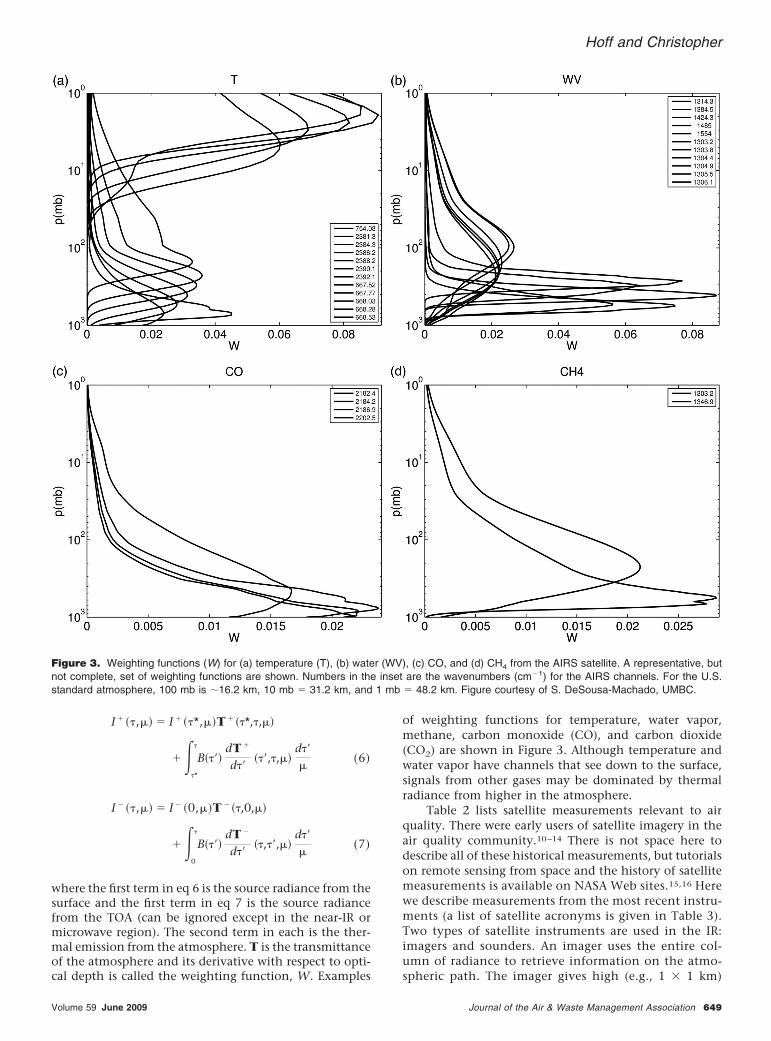
where the first term in eq 6 is the source radiance from thesurface and the first term in eq 7 is the source radiancefrom the TOA (can be ignored except in the near-IR ormicrowave region). The second term in each is the ther-mal emission from the atmosphere. T is the transmittanceof the atmosphere and its derivative with respect to opti-cal depth is called the weighting function, W. Examples

of weighting functions for temperature, water vapor,methane, carbon monoxide (CO), and carbon dioxide(CO2) are shown in Figure 3. Although temperature andwater vapor have channels that see down to the surface,signals from other gases may be dominated by thermalradiance from higher in the atmosphere.

Table 2 lists satellite measurements relevant to airquality. There were early users of satellite imagery in theair quality community.10–14 There is not space here todescribe all of these historical measurements, but tutorialson remote sensing from space and the history of satellitemeasurements is available on NASA Web sites.15,16 Herewe describe measurements from the most recent instru-ments (a list of satellite acronyms is given in Table 3).Two types of satellite instruments are used in the IR:imagers and sounders. An imager uses the entire col-umn of radiance to retrieve information on the atmo-spheric path. The imager gives high (e.g., 1 � 1 km)

Figure 3. Weighting functions (W) for (a) temperature (T), (b) water (WV), (c) CO, and (d) CH4 from the AIRS satellite. A representative, butnot complete, set of weighting functions are shown. Numbers in the inset are the wavenumbers (cm�1) for the AIRS channels. For the U.S.standard atmosphere, 100 mb is �16.2 km, 10 mb � 31.2 km, and 1 mb � 48.2 km. Figure courtesy of S. DeSousa-Machado, UMBC.



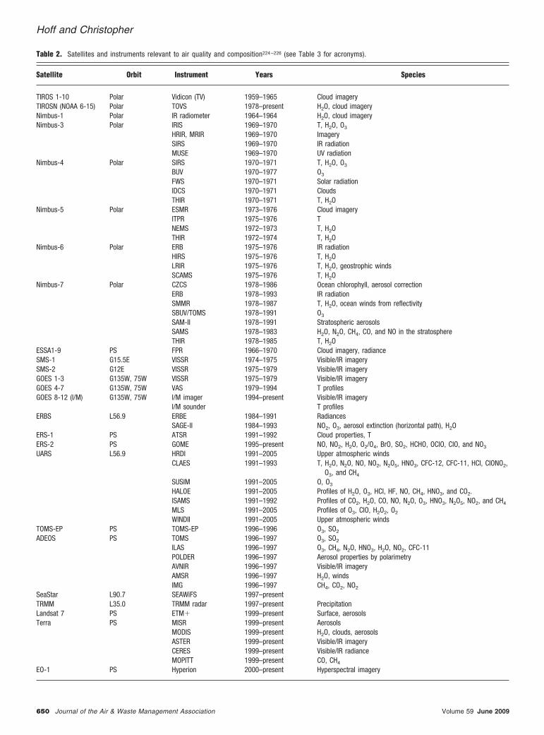
Table 2. Satellites and instruments relevant to air quality and composition224 –226 (see Table 3 for acronyms).

Satellite Orbit Instrument Years Species

TIROS 1-10 Polar Vidicon (TV) 1959–1965 Cloud imageryTIROSN (NOAA 6-15) Polar TOVS 1978–present H2O, cloud imageryNimbus-1 Polar IR radiometer 1964–1964 H2O, cloud imageryNimbus-3 Polar IRIS 1969–1970 T, H2O, O3

HRIR, MRIR 1969–1970 ImagerySIRS 1969–1970 IR radiationMUSE 1969–1970 UV radiation

Nimbus-4 Polar SIRS 1970–1971 T, H2O, O3

BUV 1970–1977 O3

FWS 1970–1971 Solar radiationIDCS 1970–1971 CloudsTHIR 1970–1971 T, H2O

Nimbus-5 Polar ESMR 1973–1976 Cloud imageryITPR 1975–1976 TNEMS 1972–1973 T, H2OTHIR 1972–1974 T, H2O

Nimbus-6 Polar ERB 1975–1976 IR radiationHIRS 1975–1976 T, H2OLRIR 1975–1976 T, H2O, geostrophic windsSCAMS 1975–1976 T, H2O

Nimbus-7 Polar CZCS 1978–1986 Ocean chlorophyll, aerosol correctionERB 1978–1993 IR radiationSMMR 1978–1987 T, H2O, ocean winds from reflectivitySBUV/TOMS 1978–1991 O3

SAM-II 1978–1991 Stratospheric aerosolsSAMS 1978–1983 H2O, N2O, CH4, CO, and NO in the stratosphereTHIR 1978–1985 T, H2O

ESSA1-9 PS FPR 1966–1970 Cloud imagery, radianceSMS-1 G15.5E VISSR 1974–1975 Visible/IR imagerySMS-2 G12E VISSR 1975–1979 Visible/IR imageryGOES 1-3 G135W, 75W VISSR 1975–1979 Visible/IR imageryGOES 4-7 G135W, 75W VAS 1979–1994 T profilesGOES 8-12 (I/M) G135W, 75W I/M imager 1994–present Visible/IR imagery

I/M sounder T profilesERBS L56.9 ERBE 1984–1991 Radiances

SAGE-II 1984–1993 NO2, O3, aerosol extinction (horizontal path), H2OERS-1 PS ATSR 1991–1992 Cloud properties, TERS-2 PS GOME 1995–present NO, NO2, H2O, O2/O4, BrO, SO2, HCHO, OClO, ClO, and NO3

UARS L56.9 HRDI 1991–2005 Upper atmospheric windsCLAES 1991–1993 T, H2O, N2O, NO, NO2, N2O5, HNO3, CFC-12, CFC-11, HCl, CIONO2,

O3, and CH4

SUSIM 1991–2005 O, O3

HALOE 1991–2005 Profiles of H2O, O3, HCl, HF, NO, CH4, HNO3, and CO2.ISAMS 1991–1992 Profiles of CO2, H2O, CO, NO, N2O, O3, HNO3, N2O5, NO2, and CH4

MLS 1991–2005 Profiles of O3, ClO, H2O2, O2

WINDII 1991–2005 Upper atmospheric windsTOMS-EP PS TOMS-EP 1996–1996 O3, SO2

ADEOS PS TOMS 1996–1997 O3, SO2

ILAS 1996–1997 O3, CH4, N2O, HNO3, H2O, NO2, CFC-11POLDER 1996–1997 Aerosol properties by polarimetryAVNIR 1996–1997 Visible/IR imageryAMSR 1996–1997 H2O, windsIMG 1996–1997 CH4, CO2, NO2

SeaStar L90.7 SEAWiFS 1997–presentTRMM L35.0 TRMM radar 1997–present PrecipitationLandsat 7 PS ETM� 1999–present Surface, aerosolsTerra PS MISR 1999–present Aerosols

MODIS 1999–present H2O, clouds, aerosolsASTER 1999–present Visible/IR imageryCERES 1999–present Visible/IR radianceMOPITT 1999–present CO, CH4

EO-1 PS Hyperion 2000–present Hyperspectral imagery



horizontal spatial information but little unambiguousvertical information.

A particular application in the IR comes where theatmosphere is transparent because there are no absorbinggases or aerosols in the scene (second term in eq 6 is zero).The radiance seen arises from the surface temperature. IRsea surface temperature (SST) instruments (AVHRR, POES,ASTER, ERS-2, AIRS) operate on this principle. Over water,the surface emissivity is approximately 0.98; however,over land the IR emissivity of the surface is a complicatedfunction of the mineral and vegetative cover and can varyfrom 0.7 to 0.98.17–19 Deriving land surface temperaturesis complicated. ASTER was designed to examine retrievalof temperature over land.19 ASTER, launched in 1998, hasrelatively coarse spectral resolution in the IR, but wasdesigned to give surface temperatures with a precision of�1.5 K and �0.015 in emissivity. Launched in 2002, AIRS

globally provides emissivity measurements at 0.05-�mspectral resolution with 3% precision from 3 to 4 �m and1% precision at 10- to 12-�m resolution.17,18 Because thesurface emissivity enters into all calculations using eq 6through the first term, emissivity uncertainty affects tracegas retrievals.

Equation 5 reduces to a linear relationship betweentemperature and microwave radiance at long wave-lengths. Microwave thermal emission penetrates clouds.Instruments such as SMMI, TRMM, TMI, and AMSR utilizemicrowave retrievals for SST measurements.

Another application of surface temperature retrievals inthe IR arises from thermal emission from fires. Measure-ments of emissions from fires have been made by “bottom-up” models (in which the areal extent of the fires, measuredfrom the ground or estimated from space-borne imagery, ismultiplied by biomass and fire-type emission factors).20

Table 2. Cont.

Satellite Orbit Instrument Years Species

SAGE-III L99.7 SAGE-III 2002–2006 Aerosols, O3, H2O, NO2

Aqua PS, A-Train AIRS 2002–present H2O, T, CH4, CO, CO2

MODIS 2002–present H2O, clouds, aerosolsAMSU 2002–present H2OAMSR/E 2002–present H2OCERES 2002–present Visible/IR radiance

ICESAT L94.0 GLAS 2003–2006 AerosolsAura PS, A-Train HRDLS 2003–present O3, H2O, CO2, CH4, NOx, HNO3, aerosols, and CFC

MLS 2003–present T, P, H2O, HNO3, O3, CO, HNO2, HCl, ClO, BrO, SO2, OHOMI 2003–present O3, SO2, NO2, aerosols, CHOCHOTES 2003–present CH4, CO, H2O, HDO, HNO3, O3, T

CALIPSO PS, A-Train CALIOP 2006–present Lidar profiles of aerosolsIIP 2006–present IR clouds

CloudSat PS, A-Train Cloudsat 2006–present Cloud radarEnvisat PS MERIS 2007–present AOD

MWR 2007–present H2OAATSR 2007–present Surface TGOMOS 2007–2009 O3, O2, NO2, NO3, UV AOD in occultationSCIAMACHY 2007–present O3, NO2, H2O, N2O, CO, CH4, CHOCHO, OClO, H2CO, SO2, aerosols,

P, TMIPAS 2007–present Trace gases

METOP PS IASI 2007–present H2O, CO2, CH, T, NO2

GOME-2 2007–present O3, aerosols, NO2, BrO, OClO, ClOAVHRR 2007–present AOD

GOSAT Polar Ibuki 2009–present CO2, GHGsOCO NA OCO 2009 failed to achieve orbit CO2

Upcoming missionsGLORY PS 2009? AerosolsADM/AEOLOS PS Aladin 2010? Lidar profiles of aerosolsGCOM-W1 PS SGGI 2013? AerosolsNPP PS 2010? AerosolsLDCM Polar 2010? AerosolsMETOP-B PS 2013?NPOESS PS 2013? AerosolsGPM 2 � PS and L39 2013–2014 PrecipitationEARTHCARE Polar ATLid 2013? Aerosols

MSI 2013? AerosolsMETOP-C PS 2016?CLARREO Polar 2016? Radiance

Notes: G12° � geostationary at 12°E longitude, PS � polar sun-synchonous, L39° � low earth orbit with a 39° inclination angle, I/M � GOES sequence of satellites from I toM, N2O5 � dinitrogen pentoxide, T � temperature, P � pressure, H2O � water, N2O � nitrous oxide, O4 � tetraoxygen, OClO � chlorine dioxide, ClO � chlorine monoxide,NO3 � nitrate radical, HF � hydrogen fluoride, H2O2, hydrogen peroxide, ClONO2 � chlorine nitrate, HCl � hydrogen chloride, GHGs � greenhouse gases, OH � hydroxyl species,CFC � chlorofluorocarbon, HNO3 � nitric acid, HNO2 � nitrous acid, HDO � deuterated water, NA � not applicable.



Other remote sensing techniques21–23 are based on the ra-diometric emissions from active fires in the 4-�m bands ofmultispectral satellites like the MODIS, the BIRD instru-ment, and the GOES. In these methods, the hypothesis isthat the heat content of fires is proportional to the massburned. Correlations between IR radiances and smoke massemission estimates are relatively high, but there further val-idation of these estimates is needed. There are factors of 10variability between emission estimates made from biomassconsumption-based smoke estimates and those from thethermal radiance techniques.23

MODIS24 and GOES/AVHRR25 fire detection algorithmsare used operationally in the detection of fire occurrences bythe U.S. Department of Agriculture (USDA) Remote SensingApplications Center26 and the National Oceanic and Atmo-spheric Administration (NOAA) National EnvironmentalSatellite, Data and Information Service (NESDIS).27 Argu-ably, fire detection in near real time is one of the mostimportant satellite inputs to air quality assessment. A historyof global fire frequency and extent is now archived at theAutomated Biomass Burning Algorithm website at the Uni-versity of Wisconsin28 and the U.S. Navy.29

Sounders invert the weighted Planck function fromthe second term in eq 6 to determine gas concentrationfrom the differential transmission. Highly absorbing gasesonly receive radiances from high in the atmosphere andweakly absorbing gases may be visible all of the way downto the surface. With the advent of highly resolved Fouriertransform spectrometers30 and grating spectrometers inorbit,31 determination of highly resolved vertical profilesof gases are possible. AIRS has been able to determinetemperature and water vapor in 1-km layers throughoutthe atmosphere. Figure 3 shows sets of weighting func-tions for temperature (Figure 3a), water vapor (Figure 3b),CO (Figure 3c) and methane (CH4; Figure 3d). The broadtrace gas weighting functions allow only a few pieces oftruly independent information to be derived from these

Table 3. Acronyms of satellites and satellite instruments.

AATSR Advanced Along Track Scanning RadiometerADEOS Advanced Earth Observation SatelliteAIRS Atmospheric Infrared SounderAMSR Advanced Microwave Scanning RadiometerAMSU Advanced Microwave Sounding Unit-AASTER Advanced Spaceborne Thermal Emission and Reflection

radiometerAtLid Atmospheric LidarATSR Along Track Scanning RadiometerAVHRR Advanced Very High Resolution RadiometerAVNIR Advanced Visible and Near-Infrared RadiometerBUV Backscatter UltravioletCALIOP Cloud and Aerosol Lidar with Orthogonal PolarizationCALIPSO Cloud and Aerosol Lidar for Pathfinder Spaceborne

ObservationsCERES Clouds and Earth’s Radiant Energy SystemCLAES Cryogenic Limb Array Etalon SpectrometerCZCS Coastal Zone Color ScannerDesDynI Deformation, Ecosystem Structure and Dynamics of IceERB Earth Radiation BudgetERBE Earth Radiation Budget ExperimentERS-2 Second European Remote-Sensing SatelliteESMR Electrically Scanning Microwave RadiometerETM Enhanced Thematic MapperFPR Flat Plate RadiometerFWS Filter Wedge SpectrometerGEOS Geodetic and Earth Orbiting SatelliteGLAS Geoscience Laser Altimeter SystemGOES Geostationary Operational Environment SatelliteGOME Global Ozone Monitoring ExperimentGOMOS Global Ozone Monitoring by Occultation of StarsHALOE Halogen Occultation ExperimentHIRDLS High-Resolution Dynamics Limb SounderHRDI High Resolution Doppler ImagerHRIR High Resolution InfraredHRIS High Resolution Infrared SounderIASI Infrared Atmospheric Sounding InterferometerICESAT Ice, Cloud, and land Elevation SatelliteIDCS Image Dissector Camera SystemILAS Improved Limb Atmospheric SpectrometerIMG ImagerIRIS Infrared Interferometer SpectrometerISAMS Improved Stratospheric and Mesospheric SounderITPR Infrared Temperature Profile RadiometerLIMS Limb Infrared Monitor of the StratosphereLITE Laser In-space Technology ExperimentLRIR Low Resolution InfraredMERIS Medium Resolution Imaging SpectrometerMIPAS Michaelson Inferometer for Passive Atmospheric SoundingMLS Microwave Limb SounderMODIS Moderate Resolution Imaging SpectroradiometerMOPITT Measurements of Pollution in the TroposphereMRIR Moderate Resolution InfraredMSI Multispectral ImagerMUSE Monitor of Ultraviolet Solar EnergyMWR Microwave RadiometerNEMS Nimbus-5 Microwave Spectrometer ExperimentNPOESS National Polar Orbiting Environmental Satellite SystemOCO Orbiting Carbon ObservatoryOMI Ozone Monitoring InstrumentPARASOL Polarization and Anisotropy of Reflectance for Atmospheric

Science coupled with Observations from a LidarPOES Polar Operational Environmental SatellitePOLDER Polarization and Directionality of the Earth ReflectancesSAGE Stratospheric Aerosol and Gas ExperimentSAM Stratospheric Aerosol Mission

Table 3. Cont.

SBUV Solar Backscatter UltravioletSCAMS Scanning Microwave SpectrometerSCIAMACHY SCanning Imaging Absorption SpectroMeter for

Atmospheric ChartographYSEAWiFs Sea-viewing Wide Field-of-view SensorsSEVERI Spinning Enhanced Visible and Infrared ImagerSIRS Satellite Infra-Red SpectrometerSMMR Scanning Multichannel Microwave RadiometerSMS Synchronous Meteorological SatelliteSSMI Special Surface Microwave ImagerSUSIM Solar Ultraviolet Spectral Irradiance MonitorTES Tropospheric Emission SpectrometerTHIR Thermal InfraredTIROS Television Infrared Observation SatelliteTMI Thermal Microwave ImagerTOMS Total Ozone Mapping SpectrometerTOMS-EP Total Ozone Mapping Spectrometer–Earth ProbeTOVS TIROS Operational Vertical SounderTRMM Tropical Rainfall Measurements MissionVAS Visible Infrared Spin Scan Radiometer Atmospheric

SounderVIIRS Visible Infrared Imager Radiometer SuiteVISSR Visible Infrared Spin Scan RadiometerWINDII Wind Imaging Interferometer



AIRS channels. For CO, it is estimated that there is reallyonly one independent weighting function from 300 to700 mb pressure altitude.32 CO2 also has only one weight-ing function, which peaks at 8-km altitude at midlatitudetemperatures but has contributions from the surface to 20km.33 More details on the theory of IR inverse methodscan be found in Goody and Yung.34

Imagers (e.g., MODIS) and sounders (e.g., AIRS) candetect aerosols in the IR for coarse-mode or mechanicallygenerated aerosols such as dust. Aerosols are possible todetect in the IR if their size is more than approximately 10�m. Particulate light scattering of solar radiation is gen-erally ignored at wavelengths greater than 1.5 �m. Atlonger wavelengths, scattering is replaced by thermalemission as the dominant source of radiation. Clouds andice can be detected from their thermal emission at highaltitudes contrasting with the surface temperature andmany of the early instruments shown in Table 2 used IRradiances to detect types of clouds. Methods exist to dis-criminate ice from water clouds using far-IR wavelengthradiance differences.35 Dust has been detected in daytimeand nighttime observations of sounders such as AIRS,36

and polar orbiting and geostationary imagers such as theMODIS and SEVIRI instruments.36–40 Although theheight of the aerosol is very important in the IR (becausethe effective temperature of the aerosol and the amountof water vapor above the dust layer must be known),optical depths retrieved in the IR have the advantage ofnot needing sunlight and therefore providing data thatare not diurnally biased. However, accurate detection andcalculation of dust aerosol properties such as opticaldepth require correct information on surface emissivity,surface temperature, water vapor, and mineralogy of thedust. Combination of instruments, such as the CALIPSOlidar (which derives aerosol height) and AIRS (which canderive AOD day and night provided the aerosol height isknown), shows promise for dust emission detection andassessment.

Passive Remote Sensing in the Visible RangeIn the UV (0.25–0.4 �m) and visible (0.4–0.7 �m) rangeof wavelengths, the Sun’s input and reflected light dom-inate the radiance being emitted back to space. There arerelatively few gases (O3, sulfur dioxide [SO2], NO2, form-aldehyde [HCHO], and glyoxal [CHOCHO]) that haveabsorption features that allow their detection at UV andvisible wavelengths. Aerosols dominate visible radiativetransfer. Because light scattering by aerosols is stronglydependent on the wavelength of light, and because theMie extinction efficiency peaks in the accumulation modebelow 1 �m in size7 (Mie scattering is largest where theparticle size and wavelength are equal), particulate matter(PM) measurements use visible wavelengths.

The differential form of the 2D radiative transferequation for visible radiation is9:

�dI��,�

d�� I��,� �

��

4�p�� ,�Ive

�

�

(8)

��

4� �0

4�

p�� ,�I��,� d�

where I is the radiance, � is zero at TOA and is a variableof the downward path, � � cos� (negative downwards), �is the single-scatter albedo, and p(� ,�) is the scatteringphase function from solid angle � to �. The equationstates that the rate of change of radiance with increasingoptical depth is related to the downwelling radiance mi-nus the lost direct radiance minus the diffuse scatteringinto 4� sr. There is a surface boundary condition for thereflected radiance9:

I��*,� � 0 �1��

0

4�

�� ,�I��*,� � 0 �� d� (9)

where � is the bidirectional reflectance distribution func-tion (BRDF) at the surface. Simplifications to the solutionarise if � is zero (black surface) or the BRDF surface isLambertian (isotropic). This is a fundamental uncertaintyin the retrieval of the optical depth. Because surfacesgenerally have non-zero and non-Lambertian BRDF, re-trieval of the AOD is an approximation.

Because p(� ,�) requires a Mie computation for aero-sols, simplified solutions such as the Eddington, two-stream, and �-Eddington approximations41 have beenwidely utilized in algorithms for satellite retrievals. Thereare no retrieval algorithms in operational use that makefull Mie calculations. In these approximations, the atmo-sphere is considered 2D plane-parallel with no effects ofclouds. The phase function is parameterized. With themultitude of complicated interactions between photonscoming downward and reflected upward, numerical solu-tions for radiative transfer are computationally intensive.In the real world of satellite retrievals, shortcuts are takenwhere a range of expected gases and aerosol types, distri-butions, and optical properties are precomputed intolook-up tables (LUTs), which are used to quickly searchfor solutions that best fit the observed radiance in orbit.42

Three-dimensional (3D) solutions are required in thepresence of clouds.43 Multiple scattering within the cloudfield, shadowing, and horizontal radiative transportwithin and between neighboring clouds are important.Recent work44–46 has examined the adjacency effect foraerosol retrievals in the presence of clouds and this effectis significant. The adjacency effect refers to the photonsscattered from the neighboring pixels into the pixel ofinterest. It will be seen later that aerosol hydration andthe radiative flux from clouds to aerosols is a significantlimitation in the retrieval of AOD. In order not to includecloud effects in AOD retrievals, cloud masks are used andthese masks have become more restrictive as the cloud-aerosol interaction effects are better understood.

Uplooking InstrumentsAlthough not satellite instruments, instruments that mea-sure the atmospheric column or optical depth from theground are instructive for what can be accomplished withremote sensing measurements. These instruments are im-portant in validating space-borne observations. The tracegas community has made column measurements of gasesfrom spectral measurements of incoming solar radiationfor almost 100 yr. The Dobson O3 spectrophotometer has



operated since the 1920s (and in its current incarnationsince 1963) by measuring the optical depth on 2–6 wave-lengths from 305 to 345 nm.47 By difference in absorptionat these wavelengths, the column of O3 can be deter-mined from Beer’s law. Because most of the absorption ofO3 occurs in the stratospheric O3 layer, this column isrelatively uniform with an optical path length of 300–400 milliatmosphere-cm (or Dobson units [DU]). Only afraction of a centimeter of pure O3 (at standard tempera-ture and pressure [STP]) protects us from solar UV radia-tion. Currently, a newer instrument, the Brewer spectro-photometer, is being used widely to measure the O3

column at 306.3, 310.1, 313.5, 316.8, and 320.1 nm.48

These wavelengths are chosen so that SO2 column retriev-als and AOD can be determined in addition to the O3

column.The AOD of the atmosphere is monitored globally at

over 90 sites with more than 4 yr of records using the Sunas a source and measuring the transmittance as a functionof solar elevation angle (or equivalently the knowledge ofthe air mass).49 The calibration of a sunphotometer isdone via the Langley regression method,50 whereby theSun’s radiance at the surface (preferably from an aerosol-free location) is measured as a function of the air mass(��1). From eq 1, the logarithm of the signal has a slopethat gives the instrumental response and an intercept (atzero air mass) that is related to the extraterrestrial solarradiance.

Sun photometers have been in use for almost 3 centu-ries.51 Major improvements in the technique over the lasthalf century have come from sensitive and stable photode-tectors, narrow band-pass filters for wavelength specificity,and robotic photometers,52–54 which can measure not onlythe direct radiation from the Sun but also the diffuse radia-tion from the sky throughout the solar hemisphere. Thescattering term, I2, in Figure 1 comes from Rayleigh and Miescattering at different angles. From multiwavelength mea-surements at numerous angles within the downwellinghemisphere of diffuse radiation, inversion techniques havebeen developed that allow determination of the particulatesize distribution at 22 radii from 0.07 to 12 �m and indicesof refraction of the scatterers.55,56

Many large networks are available globally that useuplooking sunphotometry (Aerosol Robotic Network[AERONET],53 Photometrie pour le Traitement Operation-nel de Normalization Satellitaire [PHOTONS],57 SKYNET,58

Multifilter Rotating Shadowband and Radiometer [MSRFR]59

and World Meteorological Organization Global AtmosphereWatch Physikalisch-Meteorologisches Observatorium Da-vos [WMO/GAW/PMOD]52). These networks serve as“truth” for satellite remote sensing because the instru-ments are stable, well-calibrated, well-characterized,56

and can use sophisticated techniques to quality assurethat clouds and noise are minimized. For space-borneremote sensing of AOD, most satellite instruments havebeen tested against sunphotometer results.60–70

Occultation and Near-Nadir ViewingAlthough Suomi’s images clearly showed clouds and theirmotion, within less than a decade after those first TIROSimages, gases and aerosols that are manmade and naturalin origin were being monitored. In the 1970s and 1980s,

the Nimbus satellites used occultation measurements toobserve aerosols at 1-�m wavelength using the Sun as asource in the SAM measurement platform.71 Occultationuses the motion of a spacecraft to observe the rising orsetting sun as the spacecraft crosses the terminator. Be-cause occultation measurements occur in long horizontalpaths through the atmosphere, the amount of absorptionis enhanced. Limb scattering measurements of O3 andwater vapor were observed at millimeter wavelengthswith the LIMS sounder.72

Some trace gases (e.g., O3, SO2, NO2, HCHO, andCHOCHO) can be detected in reflected UV/visible radi-ances. The strong Hartley absorption band of O3 is usedfor differentially determining the transmittance at 0.3–0.35 �m. In 1987, the SBUV Instrument detected the O3

hole over Antarctica by measuring the attenuation in thenear UV.73 A BUV instrument utilizes the strong Rayleighscattering of the atmosphere itself as a diffuse source ofradiation from above the surface. The Rayleigh scatteredphotons are then absorbed by overlying gases and spec-trally resolved through differential absorption. The detec-tion of decreases in this column to levels below 100 DU inAntarctica were made in the 1980s from a satellite instru-ment, TOMS.73 The iconic image of the low O3 column ina large vortex over Antarctica was instrumental in mobi-lizing scientific and public opinion to reduce the produc-tion of chlorofluorocarbons in the 1980s. Although thosecolumn measurements were not related to surface con-centrations of O3, the value of column measurementsto policy-making was demonstrated from a space-borneplatform.

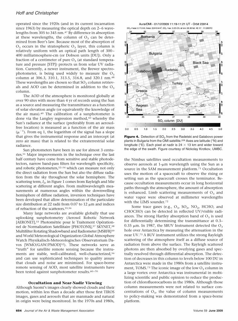
Figure 4. Detection of SO2 from the Radetski and Galabovo powerplants in Bulgaria from the OMI satellite.228 Axes are latitude (°N) andlongitude (°E). Each pixel at nadir is 24 � 13 km and wider towardthe edge of the swath. Figure courtesy of Nickolay Krotkov, UMBC.



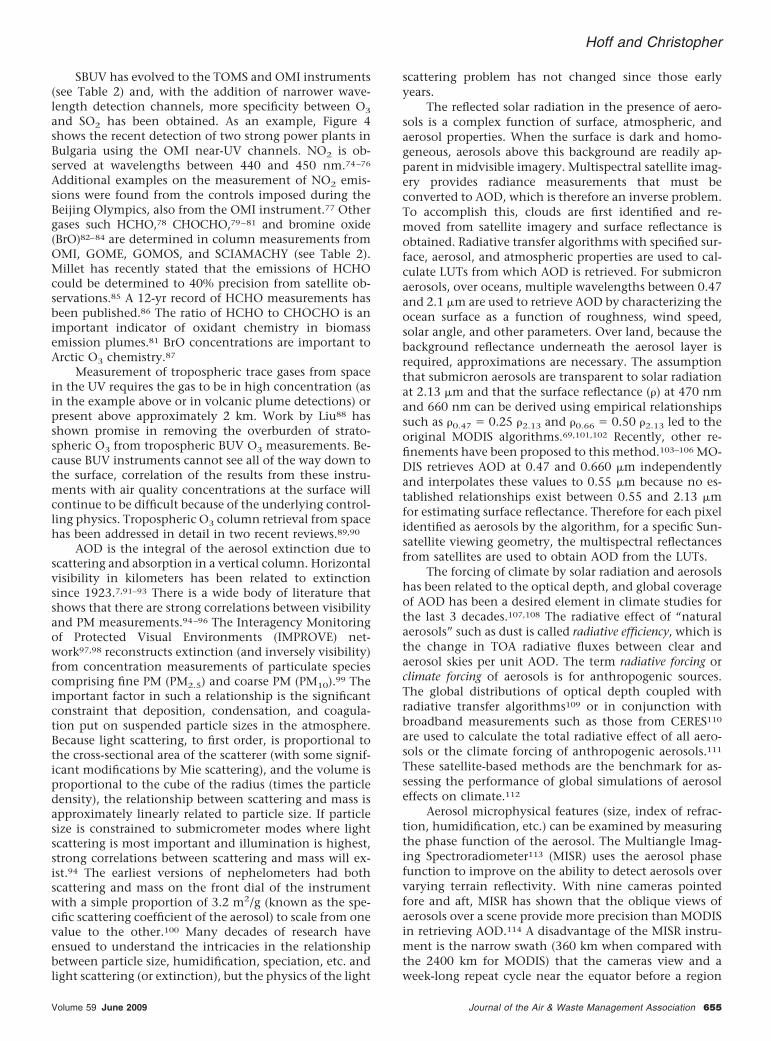
SBUV has evolved to the TOMS and OMI instruments(see Table 2) and, with the addition of narrower wave-length detection channels, more specificity between O3

and SO2 has been obtained. As an example, Figure 4shows the recent detection of two strong power plants inBulgaria using the OMI near-UV channels. NO2 is ob-served at wavelengths between 440 and 450 nm.74–76

Additional examples on the measurement of NO2 emis-sions were found from the controls imposed during theBeijing Olympics, also from the OMI instrument.77 Othergases such HCHO,78 CHOCHO,79–81 and bromine oxide(BrO)82–84 are determined in column measurements fromOMI, GOME, GOMOS, and SCIAMACHY (see Table 2).Millet has recently stated that the emissions of HCHOcould be determined to 40% precision from satellite ob-servations.85 A 12-yr record of HCHO measurements hasbeen published.86 The ratio of HCHO to CHOCHO is animportant indicator of oxidant chemistry in biomassemission plumes.81 BrO concentrations are important toArctic O3 chemistry.87

Measurement of tropospheric trace gases from spacein the UV requires the gas to be in high concentration (asin the example above or in volcanic plume detections) orpresent above approximately 2 km. Work by Liu88 hasshown promise in removing the overburden of strato-spheric O3 from tropospheric BUV O3 measurements. Be-cause BUV instruments cannot see all of the way down tothe surface, correlation of the results from these instru-ments with air quality concentrations at the surface willcontinue to be difficult because of the underlying control-ling physics. Tropospheric O3 column retrieval from spacehas been addressed in detail in two recent reviews.89,90

AOD is the integral of the aerosol extinction due toscattering and absorption in a vertical column. Horizontalvisibility in kilometers has been related to extinctionsince 1923.7,91–93 There is a wide body of literature thatshows that there are strong correlations between visibilityand PM measurements.94–96 The Interagency Monitoringof Protected Visual Environments (IMPROVE) net-work97,98 reconstructs extinction (and inversely visibility)from concentration measurements of particulate speciescomprising fine PM (PM2.5) and coarse PM (PM10).99 Theimportant factor in such a relationship is the significantconstraint that deposition, condensation, and coagula-tion put on suspended particle sizes in the atmosphere.Because light scattering, to first order, is proportional tothe cross-sectional area of the scatterer (with some signif-icant modifications by Mie scattering), and the volume isproportional to the cube of the radius (times the particledensity), the relationship between scattering and mass isapproximately linearly related to particle size. If particlesize is constrained to submicrometer modes where lightscattering is most important and illumination is highest,strong correlations between scattering and mass will ex-ist.94 The earliest versions of nephelometers had bothscattering and mass on the front dial of the instrumentwith a simple proportion of 3.2 m2/g (known as the spe-cific scattering coefficient of the aerosol) to scale from onevalue to the other.100 Many decades of research haveensued to understand the intricacies in the relationshipbetween particle size, humidification, speciation, etc. andlight scattering (or extinction), but the physics of the light

scattering problem has not changed since those earlyyears.

The reflected solar radiation in the presence of aero-sols is a complex function of surface, atmospheric, andaerosol properties. When the surface is dark and homo-geneous, aerosols above this background are readily ap-parent in midvisible imagery. Multispectral satellite imag-ery provides radiance measurements that must beconverted to AOD, which is therefore an inverse problem.To accomplish this, clouds are first identified and re-moved from satellite imagery and surface reflectance isobtained. Radiative transfer algorithms with specified sur-face, aerosol, and atmospheric properties are used to cal-culate LUTs from which AOD is retrieved. For submicronaerosols, over oceans, multiple wavelengths between 0.47and 2.1 �m are used to retrieve AOD by characterizing theocean surface as a function of roughness, wind speed,solar angle, and other parameters. Over land, because thebackground reflectance underneath the aerosol layer isrequired, approximations are necessary. The assumptionthat submicron aerosols are transparent to solar radiationat 2.13 �m and that the surface reflectance (�) at 470 nmand 660 nm can be derived using empirical relationshipssuch as �0.47 � 0.25 �2.13 and �0.66 � 0.50 �2.13 led to theoriginal MODIS algorithms.69,101,102 Recently, other re-finements have been proposed to this method.103–106 MO-DIS retrieves AOD at 0.47 and 0.660 �m independentlyand interpolates these values to 0.55 �m because no es-tablished relationships exist between 0.55 and 2.13 �mfor estimating surface reflectance. Therefore for each pixelidentified as aerosols by the algorithm, for a specific Sun-satellite viewing geometry, the multispectral reflectancesfrom satellites are used to obtain AOD from the LUTs.

The forcing of climate by solar radiation and aerosolshas been related to the optical depth, and global coverageof AOD has been a desired element in climate studies forthe last 3 decades.107,108 The radiative effect of “naturalaerosols” such as dust is called radiative efficiency, which isthe change in TOA radiative fluxes between clear andaerosol skies per unit AOD. The term radiative forcing orclimate forcing of aerosols is for anthropogenic sources.The global distributions of optical depth coupled withradiative transfer algorithms109 or in conjunction withbroadband measurements such as those from CERES110

are used to calculate the total radiative effect of all aero-sols or the climate forcing of anthropogenic aerosols.111

These satellite-based methods are the benchmark for as-sessing the performance of global simulations of aerosoleffects on climate.112

Aerosol microphysical features (size, index of refrac-tion, humidification, etc.) can be examined by measuringthe phase function of the aerosol. The Multiangle Imag-ing Spectroradiometer113 (MISR) uses the aerosol phasefunction to improve on the ability to detect aerosols overvarying terrain reflectivity. With nine cameras pointedfore and aft, MISR has shown that the oblique views ofaerosols over a scene provide more precision than MODISin retrieving AOD.114 A disadvantage of the MISR instru-ment is the narrow swath (360 km when compared withthe 2400 km for MODIS) that the cameras view and aweek-long repeat cycle near the equator before a region



can be surveyed. Therefore, MISR has less ability thanMODIS to fill the gaps between ground sensors.

The POLDER series of satellites, including the currentPARASOL instrument in the A-Train, has a strong heritageof retrieving AOD.115–121 Because the Mie scattering phasefunction of the aerosol is dependent on all of the intrinsicfactors, measurement of the angular scattering behaviorof sunlight from the aerosol can be an effective alternativeto retrieving AOD. In the POLDER class of instruments,aerosol polarimetry is used to measure the phase functionof the aerosol in backscatter. Measuring the polarizedcomponents of reflected light from the aerosol provides ameans of determining the aerosol scattering phase func-tion. The fringes in the polarimeter’s scene have spacingsthat are related to particle size and index of refraction.This technique will be used in the upcoming Glory mis-sion122 scheduled to be launched this fall by NASA. Aero-sol retrievals during the Glory mission will move beyondonly the retrievals of AOD and other parameters such asparticle size. Using both the radiance measurements inmultiple bands, the Stokes parameters that describe thepolarization state of the reflected radiation and mul-tiangle measurements will increase the number of inde-pendent variables that can be retrieved. Spectral opticalthickness, particle size, particle shape, single scatteringalbedo, and spectral behavior of the aerosol refractiveindex will be obtained.

There are other measures in addition to the AOD thatare useful in determining intrinsic aerosol properties. TheGOME and OMI instruments have a product to measurethe aerosol absorption optical depth (AAOD).123,124 Lesssensitive to the surface than the OMI AOD or aerosolindex (AI) product, the AAOD is very sensitive to blackcarbon (BC) in aerosols and has been used to detect smokeaerosol plumes. Although this product is useful for plumedelineation and transport, the AAOD may still be lesssensitive at the surface because of the atmospheric opacitydue to Rayleigh scattering. This needs to be further testedto see if it is useful for ground-based PM assessment.

Active Remote Sensing from Space and theGround (Lidar)

Lidar measures the backscatter coefficient of the aerosol.The lidar backscatter coefficient may be sufficient to de-termine the aerosol profile. In principle, lidar can be usedto infer the vertical profile of extinction and then inte-grate to obtain the optical depth. However, the returnedsignal is not only proportional to the backscatter coeffi-cient of the aerosol but also to the two-way transmittanceout to that range and back. For a single wavelength back-scatter lidar, the backscatter and total extinction (scatter-ing plus absorption) must be known. With the use of a“lidar ratio” between backscatter and absorption, it ispossible to derive an extinction profile.125 Some research-ers use the optical depth as a constraint to determine thelidar ratio. This “weights” the extinction within the lidarprofile such that stronger extinction gets preferentiallydetected. Circular reasoning results from trying to deter-mine optical depth by using an optical depth.

Raman scattering by nitrogen (N2) in the atmosphere(the profile of which is well known) can enable an exactdetermination of the extinction as a function of

height.126 This technique is used in the European AerosolResearch Lidar Network to Establish an Aerosol Climatol-ogy (EARLINET) lidar network in Europe with a significantliterature describing these measurements.127–129

Because the measurement of extinction in a columnis closely related to the scattering coefficient (if absorp-tion is a small fraction of the extinction, which is gener-ally true for sulfates), the derivation of PM2.5 from extinc-tion is similar to the nephelometer estimates discussedabove. In principle, lidar profiles may be as useful (ormore useful) than a column measurement because onecould examine the extinction closest to the surface ratherthan integrated over the observation path.

In 1994, NASA launched the LITE on the Space Shut-tle Discovery.130,131 For a 9-day period, clouds and aero-sols were observed with unprecedented detail. Detectionof desert dust, biogenic, anthropogenic, and sea-salt aero-sols were mapped over the period with 30-m verticalresolution. In a grand finale, the LITE instrument wasoperated for five orbital passes over the Atlantic Oceangiving a picture of Saharan dust transport to the UnitedStates. The LITE experiment showed that a laser could beoperated in space for extended periods and gave us a viewof aerosol spatial extent that was not previously available.

In 2003, NASA launched the GLAS132 on the ICESATsatellite. The prime focus of the mission was to measureice sheets around the globe with centimeter-scale preci-sion on the height of those surfaces. To ensure thatclouds, snow, and ice crystals were not detected as the icesurface, GLAS had two wavelength (532 and 1064 nm)profiling channels that were used for detection of cloudsand aerosols. Operating over a 5-yr period, GLAS obtainedperiods of up to a month duration, each of which hadsensitivity similar to the LITE lidar. GLAS lasers wereoperated near their rated capacity and power on the in-strument degraded quickly. The useful lifetime of thelasers for detecting clouds and aerosols was approximately90 days of continuous operation, and although GLAScarried on with its primary mission of measuring ice, theuse of GLAS for air quality purposes was limited.133,134

GLAS data were used to measure the transport of largefires in California in 2003 toward the U.S. northeast andover the ocean to Europe.135 From the GLAS measure-ments, the optical depth of this fire plume over Maine was0.48, the Angstrom coefficient was 1.8, and a mass fluxestimate of the amount of smoke in the plume was 900 �350 t � sec�1 heading eastward toward Europe.

In 2006, the CALIPSO satellite was launched in a sun-synchronous polar orbit. In a station-keeping orbit with asuite of other Earth observing satellites called the A-Train(because these satellites are led by the AQUA satellite andtrailed by the AURA satellite), CALIPSO provides continuousobservation of the planet with 30-m vertical resolution andone 70-m diameter spot every 330 m horizontally along theground track.136 The CALIPSO laser is less powerful thanLITE and in a 705-km instead of 260-km orbit. This leads tosignificantly higher noise and lower signal than was seen inthe LITE experiment. CALIPSO’s observations are much bet-ter at night when the solar background is absent than theyare in the daytime. Comparison to the AOD retrievals fromthe MODIS or GASP instruments requires daytime data.Significant averaging to improve the signal to noise ratio



(S/N) and products are available as profiles with 5- and40-km horizontal resolution. Aerosol and clouds are identi-fied in a feature finder at 330-m (single shot) and 1-, 5-, 20-,40-, and 80-km resolutions using a technique called “over-painting.” The signal is averaged for 80 km to detect thefaintest layers of aerosol and then at 40-, 20-, 5-, and 1-kmresolution more and more intense features are painted overthe weaker ones.

CALIPSO is now producing a provisional (beta) prod-uct that provides extinction profiles at 40-km horizontalscale as well as a layer extinction product at 5-km hori-zontal spatial scale.137 There is evidence that the 40-kmprofile product is not reproducing optical depth well incomparison with MODIS, with an underestimate in theCALIPSO AOD.138 Comparisons with MODIS AOD andthe CALIPSO AOD from the 5-km layer product139 suggestthat the two products are within 20% of each other onaverage when globally aggregated at 2° � 2° horizontalresolution. At this time, however, AOD results fromCALIPSO have not compared well to surface measure-ments and the reasons for the discrepancies are beingevaluated.

SATELLITE OBSERVATIONS FOR AIR QUALITYMONITORINGSeveral reviews89,90,101 examine observations of trace gasspecies and aerosols from space. The 1999 review of King etal.101 focused on the use of satellite retrievals of aerosolproperties for radiative forcing and climate applications.Nearly 10 yr later, their conclusions still hold about the needfor more precision in satellite measurements and morebreadth of measurements as a requirement to address globalaerosol forcing. Proponents of the use of satellite measure-ments make several suppositions about the usefulness ofsatellite data for air quality applications. Fishman et al.89

lead with an assertion “Geostationary satellite observationsof chemically reactive trace gases will provide unique insightinto the evolution and extent of air pollution with thetemporal resolution necessary to address air quality on adaily basis.” Those authors explain the opportunities andlimitations for measuring O3, CO, HCHO, and NO2 fromspace. They conclude with the recommendation from theNational Research Council (NRC) Decadal Survey thatgeostationary observations are of highest priority to bringsatellite composition measurements into a decision-makingframework. Martin90 reviews the methods of determiningthe four gases above but also includes a discussion of theretrieval of IR active gases, SO2, and aerosols. The focus ofthat review is largely methodological but discusses issues ofnear-surface (boundary layer) retrievals, validation needs,improvement in the algorithms used to retrieve composi-tion, and the assimilation of satellite data into large-scalenumerical models. He concludes, also quoting the NRC re-port, “These recommendations include development of ageostationary mission to provide continuous observations,to improve air quality forecasts, monitor pollutant emis-sions, and to understand pollutant transport. High priorityshould be given to supporting the next generation of satel-lite observations.”

In the NRC report and these reviews, the diversity of airquality information needs is often blurred. Near-real-timeforecasting of O3 and PM, identification of large-scale, long-

range transport (LRT) events, source identification, long-term composition measurements, regulatory compliance,management of haze impairment in Class I areas, and ex-posure measurements for health concerns are all air quality-related issues. Not all of these can be addressed by satelliteair quality measurements and, at this time, few are. Thereare significant temporal- and spatial-scale differences be-tween those needs. Chow et al.140,141 have addressed thedichotomy between health exposure assessment needs andthe scales of aerosol measurements needed by air qualityagencies. They identified implementation of a standard,compliance with air quality standards, alerts, atmosphericprocess research, determination of health effects, ecologicaleffects, and visibility impairments as reasons for the forma-tion and maintenance of an air quality monitoring system.They said that not all of these needs are compatible. Healthexposure needs tend to focus on spatial scales ranging from1 to 100 m and time scales of minutes to months. Neithersurface network monitoring or satellite measurements candeal with that spatial scale. Satellite measurements of airquality begin generally at the 4- to 10-km horizontal spatialscale. Polar orbiting measurements are nearly instantaneousand represent only one or two measurements per day in anylocation. Geostationary satellite data can be averaged tohourly or daily values because many observations are madeat a given point on the ground, thus the recommendationsabove that geostationary satellite data observations shouldbe further developed.

Air quality compliance, atmospheric compositionand trends, alerts, near-real-time forecasting, and deter-mination of visibility impairment are addressed in somefashion by satellite measurements.

Enforcement of Standards and Compliance withAir Quality Standards

In 2007, the A&WMA Critical Review by Bachmann dis-cussed the history of the National Ambient Air Quality Stan-dards (NAAQS).142 The 39-yr history of those standards par-allels the time period that satellite meteorology andobservations have developed and yet, to date, no satellitemeasurements have been used to quantitatively address theNAAQS. From the review conducted here, only one congres-sional statute has been identified, which addresses the use ofsatellite measurements for air quality purposes. NASA is em-powered with a regulatory requirement under Title VI of theClean Air Act to monitor the stratospheric O3 layer. This ruleprovides NASA with the legislative requirement for instru-ments such as the OMI monitoring the stratospheric O3

column. There are no clear legislative mandates for anyagency to do satellite monitoring climate and NASA, NOAA,the U.S. Environmental Protection Agency (EPA), and theU.S. Department of Energy (DOE) are all claiming some rolein observing climate. In congressional testimony, one of theauthors of the Decadal Survey told congress in March 2009,that “Our ability as a nation to sustain climate observationshas been complicated by the fact that no single agency hasboth the mandate and requisite budget for providing ongo-ing climate observations.”143 That testimony called for re-ferral of issues of jurisdiction in satellite measurements tothe Intergovernmental Working Group on Global Earth Ob-servations. The exact same concern can be voiced by chang-ing the word “climate” to “air quality” above.



EPA has taken a satellite observations role for itself inthe Exceptional Events Rule.144 If a region can show con-clusively that they are being impacted by an event (a fire,a dust storm, etc.) that is outside of their jurisdiction toregulate, the event can be flagged as a nonexceedanceevent. This provides a significant motivation for regionalair quality districts to examine transport from other areasto see whether there are such extenuating circumstances.The rule states:

“Information demonstrating the occurrenceof the event and its subsequent transport tothe affected monitors. This could include, forinstance, documentation from land owners/managers, satellite-derived pixels (portions ofdigital images) indicating the presence of fires;satellite images of the dispersing smoke andsmoke plume transport or trajectory calcula-tions (calculations to determine the direction oftransport of pollutant emissions from their pointof origin) connecting fires with the receptors.”

AOD tracking from day to day can provide evidencethat may help make such a case. However, there is theonus to show that the event was significant enough thathad it not occurred (the “but for” test), the site wouldhave been in compliance with the EPA air quality guide-lines. We examine next the precision of satellite surrogatemeasurements of PM2.5 as they might apply to the “butfor” test.

The Gaps in DataRural versus Urban Measurements and Spatial Holes in theSurface Networks. As of 2007, EPA’s Air Quality System(AQS) consists of 947 filter-based daily and 591 continu-ous stations run by federal, state, local, and tribal agen-cies.145 For real-time forecasting requirements, there aresignificant portions of the United States that have nocontinuous monitors. Most real-time monitors in air qual-ity networks are urban-based. These measurements focuson high-density urban sources (transportation, industry,etc.). For measurements of regional haze and complianceover longer term measurements, IMPROVE,146 the Chem-ical Speciation Network (CSN),145 the Clean Air StatusTrends Network (CASTNET),147 and the SoutheasternAerosol Research and Characterization Study (SEARCH)148

networks provide data with more regional and nationalperspective. In the EPA planning documents for PM andother criteria pollutants, effort was placed on adding non-urban sites to the NAAQS networks, especially CASTNET.149

It was suggested that perhaps 25% of the stations for O3

should be rural to avoid titration issues from nitric oxide(NO) from the cities and document regional conditions.

Because it is available in near real time, satellite in-formation can been used to alleviate these gaps betweensensors. Al-Saadi et al.150 mapped the smoke plumes em-anating from fires in the U.S. northwest in September2007. Figure 5 shows an example of where there were gapsin real-time surface measurements in Kansas, Oklahoma,and Arkansas. In all four panels, clouds are shown inwhite/gray from the MODIS visible imagery. The spatialdistribution of AOD is overlaid on the cloud image, in

which low values are in blue and high values showinghigh concentrations of pollution in orange and red. Thevertical bars in various colors denote the PM2.5 air qualityby EPA category. The plume from the Washington statefires had first been detected in AIRNow observations onSeptember 10 over the Great Lakes. On September 11, partof this plume turned southward and looped through thesouthern United States before heading eastward again. OnSeptember 11, a major branch of this plume fell betweenthe AIRNow stations in Texas and Louisiana. On Septem-ber 12 and 13, the plume was observed over much of theEast Coast. Al-Saadi used a Bayesian technique to bridgethe gap between AIRNow data that were available for theU.S. East Coast.

This example shows that satellite observations canplay a part in the “alert” role for air quality monitoring.Because the AOD data product is available 1–3 hr afterthe overpass of the satellite, air quality forecasters andanalysts have increasingly been interested in havingsuch tools available. Training sessions on how to accessthese data have been given at the EPA/National Associ-ation of Clean Air Agencies (NACAA) National Air Qual-ity Conference.151

Although satellite imagery coupled with ground in-formation is useful for qualitatively assessing PM2.5, theabovementioned example shows the utility of satellitedata filling in the gaps where there are no ground moni-tors or minimal coverage. Therefore, in the next sectionwe discuss how the satellite AOD has been comparedquantitatively with ground-based PM2.5 over various lo-cations worldwide to see whether satellite informationcan be used as a proxy.

Use of AOD to Assess Ground-BasedConcentrations: PM2.5/AOD Relationships

AOD is correlated with ground-based PM2.5 mass. Assum-ing cloud-free skies, well-mixed boundary layer of height(H) with no overlying aerosols, and aerosols that havesimilar optical properties, the AOD can be written as152:

AOD � PM2.5 H f�RH3Qext,dry

4� reff� PM2.5 H S (10)

where f(RH) is the ratio of ambient and dry extinctioncoefficients, � is the aerosol mass density (g � m�3), Qext-

,dry is the Mie extinction efficiency, and reff is the particleeffective radius (the ratio of the third to second momentsof the size distribution). S is the specific extinction effi-ciency (m2 � g�1) of the aerosol at ambient relative hu-midity (RH).

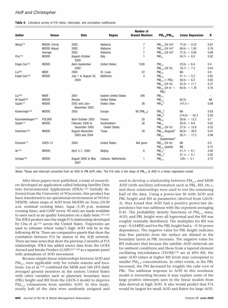
In reviewing the more than 30 papers that have ad-dressed this topic, the columnar satellite-derived AODshave been compared with surface PM2.5 mass measure-ments on a station-by-station basis. Most papers haveaddressed PM2.5/AOD and a few PM10/AOD. The resultsfrom these studies are compared in Table 4. Matchups inthe spatial location have been typically restricted to lessthan 50-km offset although there is variability in how thecollocation of the data has been done by investigators.MODIS AOD retrievals are at 10- by 10-km spatial scalesand PM2.5 ground measurements are point measurements



with a high temporal resolution. At a 10-km � hr�1 windspeed, it takes the aerosol 1 hr to cross a pixel. Thiscorresponds to hourly surface measurements. MODISAOD results have been compared with both hourly and24-hr PM2.5 measurements. More sophisticated ap-proaches use meteorological and surface information tofurther refine this relationship.

Early in the MODIS aerosol mission, Chu et al.153

found that the correlation between PM10 and AOD washigh for a single site in northern Italy. The ratio of PM2.5

to AOD (P/A) ratio was 54.7 �g � m�3 with a linear corre-lation coefficient (R) of 0.82. The predominance of thepapers below reported R, not R2, which is a measure of thevariance of the data.

Wang and Christopher’s154 study in Jefferson County,AL compared the AOD results from the Terra and Aquasatellites and 1- and 24-hr averaged PM2.5 mass from 7locations within 100 km. Linear correlation coefficientscombined from all seven sites between AOD and PM2.5 forhourly data were 0.70, and when aggregated to dailymeans the correlations increased to 0.98.

Hutchison155,156 showed the use of MODIS AOD andimagery for a dust event in Texas in 2002 and a haze eventin September of the same year but P/A correlations were

not assessed. The Texas Commission on EnvironmentalQuality (TCEQ) uses MODIS AOD and imagery to assessair quality and transport of pollutants. Hutchison etal.157–159 improved the existing P/A correlations by betteraddressing the cloud masking in MODIS and taking intoaccount the vertical profile of aerosols.

In 2004–2006, in a series of papers that covered re-gional measurements to national measurements, Engel-Cox et al.160–163 examined the linear regression of P/A. Inthe first study to look at the entire United States theyshowed that the correlations in P/A had a systematicbehavior with the best correlations coming in the U.S.northeast (correlation coefficients �0.8) and the poorestin the U.S. northwest (correlation coefficients �0.2).161

The conclusions were that where the aerosol type, mixingheight, and loading were the most uniform (the east), theP/A correlation could have a regression coefficient ofgreater than 0.8–0.9. In the west, the correlations werepoorer because of a wider variation in aerosol types (morenitrate than sulfate), more smoke than the east, highersurface reflectivities making AOD retrieval difficult, andmore elevated plumes in the AOD signatures. These re-sults are shown in Figure 6.

Figure 5. Example of MODIS gap filling from a smoke plume that was generated in Washington but impacted the southeastern United Stateson (a) September 9, (b) September 10, (c) September 11, and (d) September 12, 2007. Clouds are shown in shades of gray in which whitedenotes an optically thick cloud. The spatial distribution of MODIS AOD is shown in color and the vertical bars are PM2.5 from the EPA networkcolor coded according to concentrations. The panel for September 10 shows that there was a region where no ground-based Speciation TrendsNetwork samplers (shown by the vertical histograms) were available but the MODIS AOD data filled in the gap. Reproduced with permission fromChu et al.229 Copyright 2008 SPIE.



After these papers were published, a team of research-ers developed an application called Infusing Satellite Datainto Environmental Applications (IDEA).164 Initially de-livered from the University of Wisconsin, this product hasbeen transferred to an operational environment at NOAA/NESDIS, where maps of AOD from MODIS on Terra (10:30a.m. nominal crossing time), Aqua (1:30 p.m. nominalcrossing time), and GASP (every 30 min) are made availableto users such as air quality forecasters on a daily basis.165,166

The IDEA product uses the single P/A relationship developedby Chu et al.153 across the United States. Trajectories areused to estimate where today’s high AOD will be in thefollowing 48 hr. There are comparative panels that show thecorrelation between P/A by station in the AQS network.There are time series that show the previous 2 months of P/Arelationships. IDEA has added source data from the GOESAerosol and Smoke Product (GASP)167,168 as a separate panelwith animations of AOD movement.

Because simple linear relationships between AOD andPM2.5 were applicable only for certain seasons and loca-tions, Liu et al.169 combined the MISR and 346 EPA dailyaveraged ground monitors in the eastern United Stateswith other variables such as planetary boundary layer(PBL) height and RH from the GEOS-3 model to improvePM2.5 estimations from satellite AOD. In this study,nearly half of the data were randomly assigned and

used to develop a relationship between PM2.5 and MISRAOD (with ancillary information such as PBL, RH, etc.),and these relationships were used to test the remaininghalf of the data. Using a power-law fit with AOD andPBL height and RH as parameters (derived from GEOS-3), they found that AOD had a positive power-law de-pendence but was sublinear with the exponent averaging0.45. The probability density functions of PM2.5 mass,AOD, and PBL height were all lognormal and the RH wasroughly normally distributed. The multiplier for RH wasexp(�0.634RH) and for the PBL height had a �0.36 powerdependence. The negative value for PBL height indicatesthat fine particles from the surface are diluted in theboundary layers as PBL increases. The negative value forRH indicates that because the satellite AOD retrievals arefor ambient conditions and those from a tapered elementoscillating microbalance (TEOM)170 are at 40% RH, thesame AOD values at higher RH levels may correspond tosmaller PM2.5 concentrations. In other words, as the PBLincreased, the PM decreased by roughly the cube root ofPBL. The sublinear response to AOD in this nonlinearmodel is interesting because it may explain some of thelarge positive intercepts seen in the linear models fromdata derived at high AOD. It also would predict that P/Awould be largest for small AOD and flatter for large AOD.

Table 4. Literature survey of P/A ratios, intercepts, and correlation coefficients.

Author Sensor Date RegionNumber of

Ground Monitors PM2.5/PM10 Linear Regression R

Wang154 MODIS (Terra) 2002 Alabama 7 PM2.5 (24 hr)a 77.0� � 0.23 0.67MODIS (Aqua) 2002 Alabama 7 PM2.5 (24 hr)a 68.6� � 1.93 0.76Average 2002 Alabama 7 PM2.5 (24 hr)a 72.3� � 0.85 0.98

Chu153 MODIS August–October2000

Italy 1 PM10 54.7� � 8.0 0.82

Engel-Cox161 MODIS April–September2002

United States 1338 PM2.5 22.6� � 6.4 0.4PM2.5 (24 hr) 18.7� � 7.5 0.43

Liu208 MISR 2003 St. Louis 22 PM2.5 NA 0.8Engel-Cox163 MODIS July 1 to August 30,

2004Baltimore 4 PM2.5 31.1� � 5.2 0.65

PM2.5 (�PBL) 48.5� � 6.2 0.65PM2.5 (24 hr) 25.3� � 11.1 0.57PM2.5 (24 hr �

PBL)64.8� � 1.76 0.76

Liu169 MISR 2001 Eastern United States 346 PM2.5 –Al-Saadi164 MODIS Review United States PM2.5 62.0� NAGupta171 MODIS 2002 and July–

November 2003Global cities 26 PM10

a 141.0 � 0.96

Koelemeijer152 MODIS 2003 Europe 88 (PM2.5) PM2.5a NA 0.63

PM10a 214.0� � 42.3 0.58

Kacenelenbogen118 POLDER April–October 2003 France 28 PM2.5 26.6� � 13.2 0.7Gupta173 MODIS February 2000 to

December 2005Southeastern

United States38 PM2.5 29.4� � 8.8 0.62

PM2.5 (24 hr) 27.5� � 15.8 0.52Hutchison158 MODIS August–November

2003 and 2004Texas 28 PM2.5 (August)a 68.8� � 39.9 0.47

PM2.5

(September)a59.7� � 17.2 0.98

Paciorek177 GOES-12 2004 United States Not given PM2.5 (24 hr) NA 0.5PM2.5 (yearly) NA 0.75

An179 MODIS April 3–7, 2005 Beijing 6 PM10a 21.7� � 6.1 0.92

PM2.5a 31.1� � 5.1 0.92

Schaap180 MODIS August 2006 to May2007

Cabauw, Netherlands 1 PM2.5 120� � 5.1 0.72

Notes: aSlope and intercept converted from an AOD to PM (A/P) ratio. The P/A ratio is the slope of PM2.5 to AOD in a linear regression model.



Moving from primarily U.S. studies to 26 cities in fivecountries, Gupta et al.171 found a high P/A ratio withappreciable offset from the aggregated data from five cit-ies (Hong Kong, Basil/Bern in Switzerland, Delhi, Sydney,and New York). Correlation coefficients were reported foreach station and when averaged over all locations, thecorrelation coefficient was 0.96. In 2007, Gupta et al.172

showed that the correlation coefficient for smoke frombush fires over Sydney varied from r values of 0.11 to 0.48,probably because of the fact that the smoke may havebeen elevated that the surface monitors did not observe.They showed that over 7 yr of measurements in the U.S.southeast, P/A slopes were similar to those found by En-gel-Cox and the range of slopes varied from 21 to 36�g � m�3.173

Van Donkelaar et al.174 showed good agreement be-tween model-predicted AOD and the measured AODwhen chemistry transport model-derived vertical struc-ture was used. The spatial correlation improved from0.36–0.37 to 0.58–0.69 when the vertical profile of aero-sol extinction was used in the AOD-PM2.5 relationship.The NASA GEOS-CHEM model predicted the aerosol mi-crophysics and the mass used in the correlations. Theauthors found a similar underestimate of surface PM2.5

using AERONET AOD (considered as a reference value) of0.59 PM2.5 from the Canadian National Air PollutionSurveillance (NAPS)/AQS network. The slope improves to0.89, removing much of the bias if California is elimi-nated from the international comparison. It is difficult tocombine these data with those of the other studies be-cause the GEOS-CHEM model is so intricately woven intothe calculation of PM2.5 in this paper.

Using the POLDER instrument,116 which is flying inthe A-Train suite of satellites, Kacenelenbogen118 reportedsimilar P/A relationships to studies that used MODIS.However, their results from 28 ground monitors in Francereport the root mean square (RMS) error on the slope was

5.3 �g � m�3 and this is one of the only reported measuresof precision of the slope estimate.

Kumar, in one of two papers reporting essentially thesame data,175,176 found that in India, the P/lnA (note thelogarithmic form) has a slope of 0.33–0.48. This is con-sistent with the finding of Liu above of a sublinear slopeof P/A, but the results are difficult to reconcile with alinear model. The paper also finds a constant in the re-gression of �62 to �72, which makes little sense at � � 1(i.e., PM would be negative).

Paciorek et al.177 studied the AOD relationship withPM2.5 using the GOES-12 GASP. This product is primarilyavailable only over the continental United States. TheGASP provides data at a higher temporal resolution (every30 min) when compared with once-a-day polar orbitingMODIS and MISR sensors. They matched the GASP AODwith nearly 100,000 data points from EPA ground moni-tors and examined their results over all 4 seasons. Simpletwo-variate regressions between AOD and PM2.5 werecompared against AOD- PM2.5 relationships adjusted forRH and PBL. Although they did not give the explicitrelationship that they used for the comparison in thepaper, they did state that they could improve the corre-lation coefficient in the P/A relationship from using justthe raw AOD data from 0.5 to 0.75 by correcting for RH,the PBL height, and seasonality.

Zhang et al.178 completed a similar adjustment forlocation and season by determining independent P/A re-lationships for MODIS on Terra and Aqua for the newCollection 5 MOD04 AOD algorithm (as well as the olderheritage Collection 4 algorithm) for each of the nine EPAair quality regions by season. The Collection 5 algorithmsare a new generation of satellite retrievals that use im-proved surface and aerosol characterization with im-proved AOD accuracies when compared with AERONET.The intent of the Zhang study is to use the seasonality andregional differences to provide more specificity in theNOAA NESDIS IDEA product than the current single rela-tionship used for the entire United States (62 �g � m�3 perunit AOD with zero intercept).

In 2007, An et al.179 compared MODIS AOD nearBeijing with ground-based PM2.5 and PM10 from the sixnetworks near the city. They also conducted CommunityMultiscale Air Quality (CMAQ) model runs (April 3–7,2005) of precursor gases and aerosols for the Beijing areain preparation for the 2008 Olympic Games. Their P/Aratio was converted from the inverse of this ratio shownin their paper and, therefore, the R value shown is on theAOD/PM2.5 ratio. Because they regressed the aerosol col-umn versus the CMAQ aerosol column, we have used2000 m (from their model runs) as the mixing height forthis value in a well-mixed boundary layer. Their resultsalso indicate that the simulated SO2 concentrations fromCMAQ and columnar AODs are well correlated withground and satellite observations respectively (r � 0.7).

Schaap et al.180 compared PM2.5 from a TEOM inCabauw, Netherlands, with AERONET and MODIS retriev-als of AOD from August 2006 to May 2007. They foundslopes in the P/A relationship of 120 �g � m�3/unit AODwhen they carefully screened 67 cases with a lidar at thesite. It should be noted, however, that the authors used a

Figure 6. Linear correlation coefficient (R, gray scale) betweendaily PM2.5 and Terra-MODIS AOD across the United States.161

Correlations are determined by regressing daily PM2.5 and satelliteAOD over 1000 ground monitors and then contouring using krigingtechniques. Axes are latitude (°N) and longitude (°W). Figure cour-tesy of J.A. Engel-Cox, Battelle Memorial Institute.



modification to the TEOM with a filter dynamics mea-surements system (FDMS) that accounts for volatile ni-trate loss from the TEOM at the standard crystal temper-ature of 40 °C. One of the authors stated that this losscould be 40% of the particulate mass in Holland.181 It isdifficult, then, to compare this result to other PM2.5 mea-surements in North America and Asia where this correc-tion has not been made.

Liu et al.,169 Paciorek et al.,177 and Kacenelenbogen etal.118 have all used eq 10 to estimate the aerosol relation-ship. Charlson et al.182 used a global value of S of 5.5m2 � g�1 (at 85% average RH) to estimate global climateforcing by aerosols. Assuming a representative PBL heightover the United States is 1.5 km, this gives a P/A of 121�g � m�3 per unit optical depth. Few of the values re-trieved in practice (Table 4) have slopes that are this large.The assumption in eq 10 that one has a well-mixedboundary layer does not often hold. Factors that lead todiffering correlations in eq 10 are types of aerosol, surfacetype, whether overlying aerosols have been removed fromthe regression, whether the aerosol is really on the sur-face, definitions of PM2.5, and satellite precision in deter-mining AOD.

Several authors have tried to address the issue ofoverlying aerosols. Engel-Cox et al.163 used lidar to deter-mine cases in the Baltimore-Washington area to screenelevated aerosols. Doing so increased the linear correla-tion coefficient slightly (�5%) but left considerable un-certainty. Al-Saadi et al.150 showed an improvement inthe correlation in P/A by using the AOD/H as the regres-sion variable, deriving H from a model prediction of thePBL height during February 2007. Correlations betweenAOD and PM2.5 over the Californian San Joaquin Valleywere improved from 0.36 to 0.75 by using this method.However, a problem arises because modelers are con-cerned about the accuracy of the current PBL predictionschemes in models183 and require the use of lidar PBLheights, when available, as a validation for the modeloutput. It is not clear whether a lidar-derived PBL heightor a model height will add more precision to the P/Aprediction.

The inexplicability of the generally positive interceptin P/A regressions deserves some examination. Thereshould be no significant PM2.5 that does not scatter somelight. Although nucleation-mode aerosols would not scat-ter much light, they also do not carry much mass per unitvolume. Dust particles can be scatterers with sufficientmass, but not in the PM2.5 size range. So having a 5- to15-�g � m�3 intercept on AOD indicates uncertainty. Ifthe intercept were negative, one might assume that theAOD has some noise in a clear atmosphere. But this is notwhat the preponderance of these studies show. One ex-planation may be seen conceptually in Figure 7, where Liuet al.169 predicted a sublinear dependence of P/A with apower-law slope of �0.45 is plotted. With positive curva-ture to the P/A relationship and such nonlinearity, muchof the variability in the linear regressions can be ex-plained by the range of P/A values sampled. Where AODis low, one might expect higher slopes (which has beenseen where RH is low or corrected).163 This behaviorwould also explain the positive intercept in the regres-sions of MODIS data. MODIS has a stated precision of

�� 0.05 � 0.2 �550, where �550 is the AOD at 550 nm.Below 0.1 AOD, MODIS’ error would be �70% of theAOD. If this nonlinear behavior is real (and this deservesmore study), one would expect a positive intercept be-cause these low AOD values would be sparse in the data-sets used in Table 4. It would also improve correlation athigher PM2.5 and higher AOD (even neglecting the addi-tional factor that instrumental precision also improves athigher values).

Gupta173 looked at two alternatives to a linear corre-lation (LC). Using a multiple linear regression (MLR) tech-nique, he allowed additional variables (PBL height, loca-tion, temperature, RH) to aid P/A assessment. This studyused 2 yr of satellite data over 85 ground monitors in thesoutheastern United States. The greatest improvement inthe correlation (from 0.6 to 0.7) between PM2.5 and AODoccurred when surface temperature was added followedby PBL height to the multiple regression equations. Be-cause both of these variables may not truly be indepen-dent (PBL height is driven by convection, which is highestat highest temperatures), it is not clear what physicalchange is happening to the scattering to improve thecorrelation.

Gupta further analyzed this relationship using neuralnetwork techniques to relate eight expected dependencieson two input variables (PM2.5 and AOD) with four hiddenvariable layers in the neural net.184 The integrated satel-lite, surface, and ancillary database contained 32,834 sam-ples. The samples were divided into testing (10%), train-ing (50%), and validation (40%) categories. The overallcorrelation for the U.S. southeast increased from 0.41 inthe LC technique to 0.7 in the MLR and 0.83 in the neuralnet for validation data. There was some skill in the neuralnet in removing some outliers (see Figure 8), but one ofthe shortcomings of the technique is that it is difficult, ifnot impossible, to discover what pathway the networkused to remove the outlying points.

Figure 7. Hypothetical example of the slopes for low and highoptical depths in which the model relationship follows Liu’s169 derivedrelationship (but scaled) PM2.5 � 60 � AOD0.45. Although the overallslope of the linear regression of all of the data is 34 �g � m�3, it couldbe as high as 50.9 for the values �1 AOD and 21.8 for values fromAOD of 1 to 2. The range of AOD observed would highly influencethe slope and intercept in a linear model.



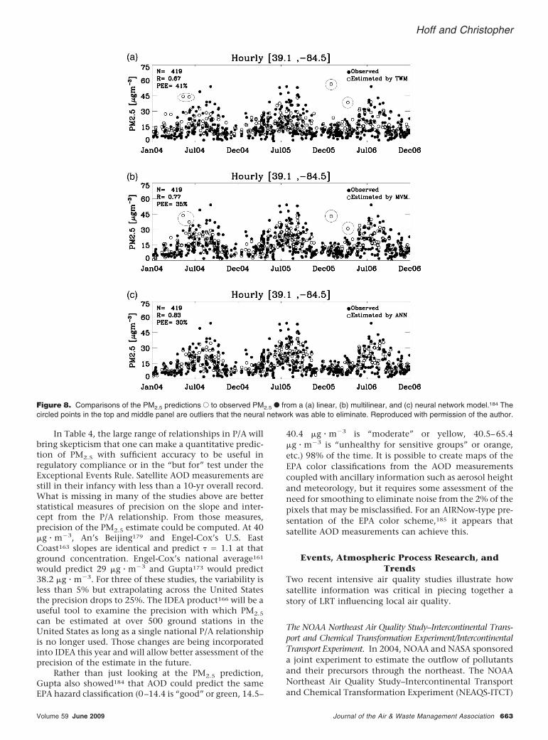
In Table 4, the large range of relationships in P/A willbring skepticism that one can make a quantitative predic-tion of PM2.5 with sufficient accuracy to be useful inregulatory compliance or in the “but for” test under theExceptional Events Rule. Satellite AOD measurements arestill in their infancy with less than a 10-yr overall record.What is missing in many of the studies above are betterstatistical measures of precision on the slope and inter-cept from the P/A relationship. From those measures,precision of the PM2.5 estimate could be computed. At 40�g � m�3, An’s Beijing179 and Engel-Cox’s U.S. EastCoast163 slopes are identical and predict � � 1.1 at thatground concentration. Engel-Cox’s national average161

would predict 29 �g � m�3 and Gupta173 would predict38.2 �g � m�3. For three of these studies, the variability isless than 5% but extrapolating across the United Statesthe precision drops to 25%. The IDEA product166 will be auseful tool to examine the precision with which PM2.5

can be estimated at over 500 ground stations in theUnited States as long as a single national P/A relationshipis no longer used. Those changes are being incorporatedinto IDEA this year and will allow better assessment of theprecision of the estimate in the future.

Rather than just looking at the PM2.5 prediction,Gupta also showed184 that AOD could predict the sameEPA hazard classification (0–14.4 is “good” or green, 14.5–

40.4 �g � m�3 is “moderate” or yellow, 40.5–65.4�g � m�3 is “unhealthy for sensitive groups” or orange,etc.) 98% of the time. It is possible to create maps of theEPA color classifications from the AOD measurementscoupled with ancillary information such as aerosol heightand meteorology, but it requires some assessment of theneed for smoothing to eliminate noise from the 2% of thepixels that may be misclassified. For an AIRNow-type pre-sentation of the EPA color scheme,185 it appears thatsatellite AOD measurements can achieve this.

Events, Atmospheric Process Research, andTrends

Two recent intensive air quality studies illustrate howsatellite information was critical in piecing together astory of LRT influencing local air quality.

The NOAA Northeast Air Quality Study–Intercontinental Trans-port and Chemical Transformation Experiment/IntercontinentalTransport Experiment. In 2004, NOAA and NASA sponsoreda joint experiment to estimate the outflow of pollutantsand their precursors through the northeast. The NOAANortheast Air Quality Study–Intercontinental Transportand Chemical Transformation Experiment (NEAQS-ITCT)

Figure 8. Comparisons of the PM2.5 predictions E to observed PM2.5 F from a (a) linear, (b) multilinear, and (c) neural network model.184 Thecircled points in the top and middle panel are outliers that the neural network was able to eliminate. Reproduced with permission of the author.



was run in conjunction with the Intercontinental Trans-port Experiment (INTEX-NA). Designed to measure out-flow of pollutants from the United States and follow thosepollutant plumes as far as Europe, the 2004 study washighly influenced from major forest fires in Alaska. Col-umn measurements of AOD and CO were consistent intracing the input of a major plume from these fires andhelped discriminate local pollution from LRT.

Analysis of this case186 showed that there was signif-icant impact of the CO from these fire plumes on INTEXDC-8 aircraft measurements made in the U.S. east includ-ing both trace gases and BC (Figure 9). Those columnmeasurements were well aloft for much of their travel tothe U.S. East Coast. In Figure 10, we have superimposed 3days of the University of Wisconsin HSRL profiles for thisperiod.186 The lidar profiled the lowest 15 km of theatmosphere and showed a large plume of material passingover Madison, WI, on July 18, 2004. Shown below theHSRL lidar data are three panels of MODIS AOD.187 TheAOD data showed that the plume passed over Wisconsinearly on July 18 and had passed through by July 19. Fiveground-based monitors making PM2.5 measurements inWisconsin are also shown in this figure and the threetimes from MODIS are noted as arrows. Although there isa slow increase of PM through the period from July 16 to20, the impact of the plume on ground-based PM wasminimal in Wisconsin. In Maryland, smoke impacted theboundary layer on July 20 in the afternoon.163,186 Thisexample shows that the column measurement is impor-tant to investigate LRT components to local pollution andthat the vertical dimension cannot be ignored. If plumesdo not contact the surface (or only mix down for limitedperiods as this plume did on July 18 evening), ground-based concentrations will not be impacted. Without hav-ing the HSRL results available, it would have been impos-sible to understand why such a large AOD plume had solittle impact on PM2.5 at the ground.

TEXAS Air Quality Study. In the 2006 second Texas AirQuality Study (TEXAQS-II), model estimates of O3 andPM2.5 were compared with measurements from an inten-sive air and ground sampling program. Although theoverall results from the study gave results that were com-parable to model predictions, there were cases in whichPM north of Houston exceeded the predictions. Whenlooked at with satellite information, dust intrusions fromthe Caribbean were shown to enhance the ground con-centrations. CALIPSO results showed that the dust wasfrom the Sahara in Africa (Figure 11 shows a multiday setof CALIPSO cross sections tracking the dust plume intothe Caribbean and up into Texas).188 In addition to theLRT import of dust, McMillan et al.189 have shown againthat fire plumes from Montana impacted the study duringthe TEXAQS period.

Trends. In the future, satellite measurements may have asignificant input in trend determination, but the timeseries for most satellites is short. There are no publishedtrends in AOD from MODIS. Xia et al.190 have publisheddata showing a weekday–weekend difference in AODfrom AERONET and MODIS. Longer-term satellite-derivedtrend data for NO2 in Europe shows a decreasing trend in

emissions that is consistent with the European Monitoringand Evaluation Programme emissions inventory.191 The in-creased emissions of NO2 in China and trends on othercontinents have been documented by Richter et al.89,192

To What Extent Does AOD Improve Modeling?Numerical modeling and forecasting of aerosols and tracegases rely on accurate emission locations. Most simula-tion frameworks require meteorological models to obtainatmospheric dynamic conditions for the period of fore-cast that is used as input to the core of a model thatrequires transport, chemistry, and deposition informa-tion.193–198 In situ and satellite datasets are useful to eval-uate these simulations.

These simulations generally capture the average spa-tial trends and the dynamic range in PM2.5 when com-pared with in situ measurements, but overestimatesand/or underestimates are possible because of various is-sues, including uncertainties in emission inventories,physics, chemistry, and meteorology.193–196 Assumptionsin boundary conditions and poorly quantified emissionswithin the model domain are among the major uncertain-ties in simulations. McKeen et al.195 evaluated seven airquality forecast models using data collected during a fieldexperiment and discussed the biases between and amongthese models. These simulations were compared against118 PM2.5 monitors and 342 O3 monitors between July14, 2004 and August 17, 2004. These studies did not usesatellite data for model verification or for assimilationpurposes. Their results showed that the PM2.5 forecastshad better skill relative to the O3 forecasts although themodels did not capture the diurnal behavior of PM2.5 inurban and rural locations.

Most of these models also do not account for aerosolstransported from outside of the model domain.193 Studiesindicate that when compared with ground truth, modelsunderestimate PM2.5 by a factor of 2 during biomass burn-ing events because of smoke transported from outside ofthe model domain.195 Satellite remote sensing can helpwith this issue because near-real-time information on firelocations and emissions are available. Hot spots/fire loca-tions are routinely identified by polar orbiting199 andgeostationary sensors25 that are then used to obtain PM2.5

emissions.20,200,201 These fire source functions can then beused to improve model forecasts. Wang et al.202 showedthe utility of using fire emissions from Central America ina forecast model to estimate PM2.5 concentrations in theUnited States. Stein et al.203 recently used the HybridSingle-Particle Lagrangian Integrated Trajectory (HYSPLIT)model to estimate PM2.5 concentrations from various fireevents. These models assess surface PM2.5 due to aerosolstransported from outside of the domain.

Satellite remote sensing products can also be assimi-lated into numerical models to improve predictive capa-bilities. For example, Mathur194 used the MODIS AODduring the 2004 fires in Alaska to improve the character-ization of pollution from outside of the model domain.For each model grid, the PM2.5 mass was estimated fromthe satellite AOD using a priori PM2.5-AOD relationships.The difference in PM2.5 between the base model runs (nofire emissions) and the PM2.5 from the satellite AOD are



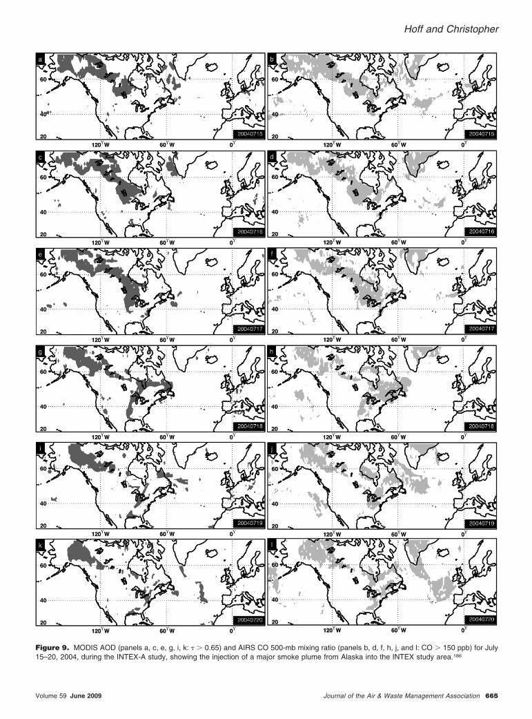
Figure 9. MODIS AOD (panels a, c, e, g, i, k: � � 0.65) and AIRS CO 500-mb mixing ratio (panels b, d, f, h, j, and l: CO � 150 ppb) for July15–20, 2004, during the INTEX-A study, showing the injection of a major smoke plume from Alaska into the INTEX study area.186



Figure 10. The same case showing (a) the University of Wisconsin HSRL lidar profiles that were based in Madison, WI; (b) the MODIS TerraAOD; and (c) the ground-based PM2.5 for five stations in Wisconsin from the AIRNow technology database. The times of the overpasses aremarked with arrows on the PM2.5 time series.

Figure 11. Injection of Saharan dust into the TEXAQS 2006 study area on August 28, 2006.188



calculated and then vertically distributed for various spe-cies for further simulations. This first attempt at simulat-ing AOD requires correct P/A relationships that are notapplicable for all meteorological situations. For example,the a priori relationship assumes that the aerosols are in awell-mixed boundary layer that yields good PM2.5/AODrelationships, but this may not be true in all cases. It alsorequires assumptions on taking column measurementsand distributing it vertically using a priori information.Another source of uncertainty arises from taking columnsatellite AOD retrievals with no speciation informationand allocating these into various species for the model.

Because the vertical distribution of aerosols is criticalfor assessing PM2.5, another technique is to take thecolumn-integrated satellite AOD and distribute it verti-cally on the basis of the model-predicted distributions ofaerosols. This assumes that the physics, chemistry, radia-tion, and the mechanics of the PBL height characteriza-tion in the model are correct.198 Probably the “best” so-lution is to take measured vertical distributions of aerosolsfrom a space-borne lidar or a ground-based lidar to parti-tion the satellite AOD into various model layers199; how-ever, there are challenges in this approach as well. TheCALIOP two-wavelength polarization-sensitive lidar (onthe CALIPSO satellite) with a footprint of 70 m does nothave global daily coverage and precludes characterizationof vertical distributions over the entire modeling domain.Also, ground-based lidars need to be available in a near-continuous manner to improve model performance.

Kondragunta et al.204 compared the CMAQ simula-tions of aerosols with GOES AOD during the summer2004 International Consortium for Atmospheric Researchon Transformation/New England Air Quality Study(ICARTT/NEAQS) field campaign. This period was domi-nated by LRT of smoke from fires in Canada/Alaska andregional-scale sulfate event over the eastern United States.The CMAQ simulations did not include boundary condi-tions for these smoke aerosols. For clear sky conditions,the GOES AOD was compared with simulated AOD. Theforecast accuracy was between 0 and 20% for exceedancesof PM2.5 (AOD � 0.55) and between 40 and 90% fornonexceedances (AOD � 0.55). In general, accuracieswere better from the sulfate events when compared withthe smoke events because the CMAQ did not includeemissions from LRT of smoke aerosols. Although someEuropean models are actively using chemical data assim-ilation,205,206 several challenges remain, including lack ofobservations about vertical structure and a better under-standing of aerosol composition, emission locations,sources, and magnitudes. In cloud-free skies, AOD is avail-able on a daily near-real-time basis that can be consideredin an assimilation system.

Detection of source emissions from event-driven andintermittent sources may be one of the greatest strengthsof satellite measurements. Measurements of emissionsfrom fires have been made by “bottom-up” models (wherethe areal extent of the fires is multiplied by emissionfactors from biomass type and fire type).20 Other tech-niques22,23 are based on the radiometric emissions fromactive fires in the 4-�m bands of multispectral satellitessuch as MODIS and GOES. Correlations of the emissionsin the IR and smoke mass are relatively high, but there is

the need for validation of these emissions and the qualityassurance of the fire detections to ensure that glint (spec-ular reflection) and other issues are dealt with.

Trace gas emissions of NO2 have been observed fromlarge urban regions. Oxides of nitrogen (NOx) and SO2

emissions have been reported from Beijing,207 and re-cently, emission controls in that region during the Olym-pics were observed from space-borne measurements.77 Ifrobust emissions data can be gleaned from satellite obser-vations, better model predictions can be expected in thefuture.

In summary, the use of satellite data products forforecasting PM2.5 in chemical models is in its infancy.Using fire locations and emissions of smoke aerosolsfrom biomass burning fires has shown success in assess-ing PM2.5. There is no reason why these datasets shouldnot be included in models. These satellite-based data-sets are especially useful for assessing PM2.5 air qualityfrom LRT.202 Near-daily retrievals of columnar AOD arealso available on a continuous basis from several satel-lites. In clear sky conditions, these data products can beused for model assessment or as input to models. Al-though ancillary information about the vertical struc-ture of aerosols is critical, space-borne and ground-based lidars provide this information when available.This is an asset that needs to be utilized for modelingstudies, especially when aerosol injection height infor-mation is needed.

FUTURE MISSIONS AND PROSPECTS FORIMPROVING ON THE PHYSICSThe examples above and the extensive literature that hasdeveloped on the use of satellite instruments for air qual-ity assessment show a promising future for the use ofthese data in air quality research and applications. But, inanswer to the title of this review, we have not yet reachedthe promised land. There are still significant issues toaddress before these measurements will be as routinelyused as a PM2.5 monitor in a network.

Some Fundamental Problems in Satellite RemoteSensing

Extrinsic versus Intrinsic Property Requirements. The use ofsatellite data needs to address the fundamental mismatchin the regulatory need to measure a mass concentration(or in the case of trace gases, a mixing ratio at the surface)from a column measurement of an optical radiance prop-erty. For trace gases, in principle, the problem is some-what easier because the conversion of mixing ratio toextinction requires the knowledge of the absorption co-efficient of the gas at a given pressure and temperature.Because many of our visible absorption measurements forO3, SO2, and NO2 are relatively wide spectral measure-ments, the absorption coefficient is reasonably wellknown and easy to characterize. For these gases, the col-umn measurement from passive instruments may be suf-ficient to characterize a mass budget, especially if inte-grated horizontally by the measurement and vertically bythe column measurement to give fluxes of the gas acrossa plane.

Aerosols provide a more difficult challenge becausethe intrinsic (or microphysical) property of the pollutant



is not constant as it is for a gas. For aerosols, the compo-sition, sizes, indices of refraction, and hydration proper-ties are not constant. Not only do the extrinsic properties(i.e., the number of particles per cubic meter, the height ofthe mixed layer, the profile, etc.) have to be known, butthe PM2.5 (or PM10) intrinsic property differences (com-position, size distribution, density, indices of refraction,hygroscopicity) is also problematic. To the extent thatPM2.5 is used in the regulatory environment, there willstill be significant scientific issues between what is mea-sured and the pollution problem (acid rain, health, etc.)that is being addressed. With that in mind, the use of anoptical surrogate for PM2.5 is probably no more challeng-ing an issue.

The use of the AOD as a measure for mass concentra-tion has skill in some regions but less in others and doesnot provide a uniform way to measure aerosols across theUnited States. We discussed in Table 4 the range of mea-surements from across the globe and the wide range ofcorrelations between AOD and mass. It may be possible toreduce that range of uncertainty by further intrinsic mea-surements. It is unlikely that we will further reduce thatuncertainty by statistical regressions. Within a given re-gion, the types of aerosols may be more limited, theheights of the boundary layer may be more uniform, theranges of humidity that the aerosol experiences morelimited, and these factors may make the correlation ofAOD to PM more accurate in some regions.163,184,208 Studyof the controlling extrinsic factors will aid in understand-ing the P/A relationship. It is not at all obvious that thesecan be extrapolated to other regions with similar certaintyof the predictability of PM2.5. However, some regions ofthe globe have no PM measurements at all. Central, SouthAmerica, and Africa have few stations measuring PM. Thecurrent uncertainty in the P/A ratios could be acceptablefor estimates in those regions.

Clouds. Clouds cover 60–70% of the planet at anytime.209,210 Clouds obscure the surface and make detec-tion of aerosols at the surface impossible. Gupta211 exam-ined this possible bias and determined that for the U.S.southeast for a 7-yr period, the PM2.5 levels on days withand without clouds have the same probability densityfunctions; yearly means have average values of PM2.5 thatdiffer by less than 2 �g � m�3. This would indicate thatclouds do not significantly bias the measurement of PM2.5

in broken cloud fields on an annual mean basis. However,cloud obscuration cannot be neglected, and satellite ob-servations cannot be used to detect exceedances for re-gions that have extensive cloud cover. This limitation issignificant during winter months at midlatitudes and dur-ing the rainy seasons in the tropics.

Snow. Similar to clouds, the high surface reflectivity ofsnow is problematic at wavelengths that rely on darksurfaces for detection of extinction contrast. NO2 retriev-als are possible over snow-covered surfaces because theNO2 absorption features are close together in wavelength(�10 nm) and, over this wavelength range, reflectivityfrom the surface is constant. OMI AAOD retrievals aresimilarly unaffected by snow or low clouds because theeffective scattering height for these UV wavelengths is 2–3

km or more. However, all other visible retrievals are pre-cluded over snow.

Bright Surfaces. Bright surfaces like deserts or bare soil donot provide enough contrast with the added radiancefrom aerosols to be able to retrieve AOD. In the “DeepBlue” algorithm,106 Hsu and her colleagues used theshortest wavelength from MODIS to push the contrastbetween the surface reflectance and aerosol reflectancebeyond the traditional MODIS AOD retrieval. Deserts andbright surfaces are still a challenge for aerosol retrievals.De Castanho and Martins63 used a “critical reflectance”method for bright surfaces (such as urban areas with hard-ened asphalt and concrete surfaces). In that method, thereis a critical reflectance for which the range of expectedAODs in a plot of reflectances at 0.65 �m crosses.212,213 If,for a given surface pixel, this critical reflectance can bedetermined, radiance ratios at higher or lower reflectivi-ties can be mapped to AODs. In other words, aerosols overbright surfaces may darken the scene, over dark surfacesbrighten the scene, and the degree to which they do so iswavelength dependent.

Lyapustin et al.214 have developed algorithms thatuse more sophistication in the knowledge from the BRDFat the surface. In a routine designed to better detect over-lying clouds, the Multiangle Implementation of Atmo-spheric Correction (MAIAC) algorithm215 uses the con-cept that the surface reflectivity is fixed and varies on timescales of days, whereas the atmosphere is moving with atime scale of minutes. Using the 2D covariance fields fromclear and hazy scenes, the algorithm is able to pick outscene elements that are atmospheric in nature over highlystructured underlying surface scenes. This technique islikely to show important new results from geostationarysensors that have more wavelength channels and showmotion over scales of minutes.

Noncontinuity in Observations. Polar orbiting satellites aregenerally placed in sun-synchronous orbits with equatorcrossing times in the morning or afternoon. At 7.1 km/secorbital velocity, observation of a 10- by 10-km MODISpixel takes 1.5 sec. At most, a given site would be observedless than 4 times per day from a polar orbiter. Althoughthese orbits are designed to be representative of the diur-nal cycle variations in the PBL, the lack of hourly obser-vations throughout the day limits the usefulness for ex-ceedances of the AQS.

The geostationary satellites—GOES-12 and GOES-11—have an AOD product that can be related to AOD.GASP measures AOD every half hour across the UnitedStates at 4- by 4-km resolution. This high temporal reso-lution allows not only visualization of aerosol plumemovement, but is also potentially useful for timing ofexceedances. GASP, however, does not have the precisionof MODIS’ AOD primarily because it has only one broadvisible channel. The GASP retrieval is based on discrimi-nation of the radiance in that channel from the minimumradiance detected over the previous 28 days of measure-ment. If the minimum in such radiance is not from a veryaerosol-free day, there will be some bias in the retrieval.By 2015, NOAA proposes to launch the GOES-R series ofsatellites. This series has MODIS-like channels and will



allow retrievals of a more precise AOD every 5–30 min,depending on the observation mode of the satellite. Thisis a factor in the Decadal Survey recommendation forgeostationary platforms quoted above.

Precision. The AOD P/A ratio, even if refined to a highdegree of correlation, still has error estimates in the liter-ature on the order of 5–10 �g � m�3/unit AOD (15–30%).It should be incumbent on future papers written aboutthis regression to include such estimates of the precision.MODIS AOD has precision42 of �0.05 � 0.2�, which in-dicates that the precision of the AOD retrieval itself dom-inates the P/A relationship. For surface networks in ClassI areas, the precision of the PM2.5 measurement should bebetter than 2 �g � m�3 or 5% and better than 10% in ClassII and Class III areas.216 Satellite measurements are not atthat level of maturity and it is unlikely that they will meetthat precision in the near future. Satellite observations ofcolumn measures of trace gases similarly will be difficultto relate to regulatory compliance needs. One exceptionto this may be NO2, for which significant correlations toground-based NOx and NOy observations can be made ifthe NO2/NOy ratio is estimated.217,218 In fact, satellitessuch as GOME, SCIAMACHY, and OMI may actually mea-sure ambient rural NO2 more completely than the groundnetworks. In 2001–2006, only 243 of 4177 site-years(�5%) of NO2 data in the United States were not inmetropolitan statistical areas.219

Errors in the AOD measurement directly propagateinto the precision with which PM can be estimated. Thereare some areas in which AOD retrievals can be improved.As in the 7–9 wavelength AERONET retrievals of aerosolsize, single scattering albedo, and indices of refraction, itmay be possible in the future with hyperspectral satelliteinstruments (hundreds of wavelengths) to develop algo-rithms with more accuracy in determining the micro-physical (intrinsic) properties of the aerosol, which wouldmake the retrieval of AOD or extinction (the extrinsicproperties) more robust. However, wavelength channelsare expensive to implement in orbit, and the futureNPOESS missions have taken the unfortunate path ofhaving fewer instead of more channels.

Combined MeasurementsCombination of sensors shows promise in reducing theuncertainty in column retrievals. Use of profiling instru-ments such as lidars from the ground and from spaceallows more certain placement of the pollutant in thevertical. For CO and CH4 algorithms, knowing the heightof the pollutant constrains the range of IR temperaturesthat affect retrievals. Similarly, dust profiling in the IRneeds an estimate of the aerosol height.36 The OMI AODcan be improved if knowledge of the plume height isknown.70 However, profiling instruments with variablepointing ability are unlikely in the next few decades sim-ply because the combination of power, agility, and weightwould make such an instrument difficult to carry to space.Without having horizontal spatial coverage (similar tothe MISR difficulty), most areas of the globe would not becovered each day and interpolation between orbits withover 1500-km spacing would cause even extended, signif-icant features to be missed because the orbit path was not

appropriate on that day. For example, during the South-ern California wildfires of October 2007, the CALIPSOsatellite detected the smoke only twice over a 7-day periodbecause of the vagaries of the orbital coverage with re-spect to the fires.166 Future lidar satellite missions shouldconsider active pointing capability to target specific sig-nificant events such as fires (natural and Homeland Secu-rity related) and volcanoes.

Measurement of the vertical humidity profile is desir-able in conjunction with an AOD retrieval. Hygroscopicgrowth can change extinction by factors of 3–5, thereforeit is expected that AOD would have a strong humidifica-tion effect (e.g., eq 10). Hygroscopic effects near the edgesof clouds is an active research topic and it may be that thehydration of aerosols can extend outward from cloudedges by up to 10 km horizontally.46 Combination ofground-based lidars and satellite measurements mayprove useful in determining the horizontal scales in-volved. Whiteman220 has proposed an airborne water va-por Raman lidar that is currently in the testing phase.Such a system is being evaluated for use from a space-borne orbit. AIRS and TES do provide profile measure-ments of water vapor in the free troposphere but havedifficulty near the surface where understanding the hy-dration of aerosols is most needed. Models can providethe information needed to better account for the hydra-tion effect of aerosols to relate to dry PM2.5.173,208

Unlike the lidar on the CALIPSO satellite, which mea-sures a broad elastic scattering feature from both Rayleighscattering and aerosol backscatter, NASA has flown a pro-totype instrument similar to the ground-based HSRLshown in Figure 10. The NASA Langley HSRL188 works bysimultaneously measuring the Rayleigh-scattered andaerosol-scattered components of elastic scattering. Theratio of these signals is proportional to the aerosol mixingratio and the extinction as a function of height. HSRLlidars are under consideration for the Atmospheric Chem-istry Experiment (ACE) mission, a part of the DecadalSurvey planned missions.

Several satellites are planned that have advancedmulticomponent profiling capability. The EuropeanSpace Agency’s Aladin wind and aerosol lidar will be thefirst to launch in 2010 on the Atmospheric DynamicsMission (ADM)-Aeolus platform and will be followed in2013 by the ATLid on the EARTHCARE mission.221,222

Although the United States plans to launch ICESAT-II inthis time frame and a lidar on the DesDynI mission, bothwill be used only for surface detection (ice and vegetation,respectively). There are no realistic plans to launch atmo-spheric lidar in NASA’s plans before the ACE mission,which cannot credibly be launched before 2020 at thecurrent NASA funding profile. This is a considerable tran-sition of capability in profiling aerosols to Europe over thenext decade.

The GOES-R series of satellites have been designed tomimic the spectral features available on MODIS or theVIIRS instruments that are run in LEO and polar orbits.The GOES-R Advanced Baseline Imager (ABI) is an impor-tant development for AOD retrievals.223 In a geostation-ary orbit, GOES-R ABI will be able to view the UnitedStates every half hour while the Sun is up. The GOES-RABI algorithm is being designed to give similar precision



to MODIS but instead of 2 realizations (MODIS Terra andMODIS Aqua) each day, we will have 14–28 images taken.For forecasting and analysis, this will revolutionize ourability to address aerosol transport and monitoring.GOES-R will not launch until 2015. It is unfortunate thatso many of the NASA Earth Observing System (EOS) in-struments are nearing or past the planned lifetime forthese instruments. If instruments start to fail in orbit, theUnited States will be poorly placed to continue in airquality monitoring from space and will have to rely on itsinternational partners.

One impediment to such combinations of datasets isthe diverse nature of the data formats, spatial and tempo-ral scale, and access. Not all satellite data, especially fromforeign agencies, are publicly available. Another impedi-ment is that satellite science teams tend to have narrowfoci with no mission funding to combine measurementsfrom other sensors.

CONCLUSIONSSatellite air quality measurements are in their infancywith 50 yr of history of atmospheric composition mea-surements but less than 10 yr of record with modernmultisensor platforms from polar and geostationary or-bits. The physics behind remote sensing of gases andaerosols uses Beer’s law to convert radiances measured inorbit to mixing ratios or concentrations. IR retrievals andvisible measurements have fundamentally different ap-proaches to solving for the concentrations. In the IR,broad weighting functions make the vertical resolution ofthe profile of the target species vary from 1 to 10 kmdepending on the gas. Horizontal resolution of the mea-surements is comparable to visible column measurements(1–10 km horizontally).

Success has been shown at retrieving the column ofseveral gases in visible and IR wavelengths (e.g., O3, NO2,SO2, HCHO, CHOCHO, BrO, water, CO, CH4, CO2). How-ever, the lowest part of the troposphere is too opticallythick to accurately measure O3 and SO2 all of the way tothe surface. Aerosols have been quantified using the AODand the relationship between AOD and PM2.5 is beingactively investigated.

Although the desire for the use of satellite data for airquality purposes is widely stated, the reality is that manyof the measurements have not yet met the promise thatthey can be operationally used for today’s air qualitymonitoring requirements. Precision in measuring AOD is�20%, and the relationship to PM2.5 is at best �30% incontrolled measurements in which overlying aerosols,aerosol type, and boundary layer structure are known.This is not currently sufficient for regulatory use. Theinterest in using such data in the EPA Exceptional EventRule needs investigation, but with the precision above,the “but for” provision in the rule makes the use of sat-ellite data possible in significant exceedances only. Appli-cations such as event identification, transport, and atmo-spheric composition determination are strengths ofsatellite measurements. Where high precision is required(compliance monitoring, the “but for” test, and quanti-tative measurement of visibility effects on Class I areas),satellite data are presently of limited utility.

Strengths of satellite measurement are found in emis-sions identification (fires especially), event tracking andtransport, definition of boundaries of large-scale pollu-tion features, and providing some evidence for profiles ofpollutants well above the surface. Satellite observationsfill gaps in areas where there are no ground sensors (e.g.,much of the third world). Satellite measurements havebeen very useful in defining production, oxidation, andevolution processes from biomass burning. Satellite imag-ery can provide iconic views of major events such as forestfires, volcanic plumes, and stagnant haze masses overhighly industrialized areas. In conveying the extent ofpollution to the public, visual imagery from space isimportant.

Combining multiple measurements and models im-proves the understanding of the physics of the measure-ment and improves the precision. Use of forecast andanalysis models is synergistic with satellite and surfacemeasurements, improving understanding of the predic-tion and the measurement. Assimilation of existing satel-lite air quality and ground data into models needs seriousevaluation, and the United States lags Europe in suchresearch. More new missions for air quality will belaunched in Europe and Japan than in the United Statesfor the next decade. Although the promise of satellitemeasurements has not been fully met at this time, space-borne remote sensing will be one way of seeing the prom-ised land.

ACKNOWLEDGMENTSThe authors thank Drs. Pawan Gupta, Jill Engel-Cox,Kevin McCann, Nickolay Krotkov, James Szykman, andWallace McMillan for providing graphics that were usedin this review. Helpful comments were received from Me-loe Kacenelenbogen and Amy Huff in early drafts of thereview. Comments of the reviewers (George Hidy, JohnWatson, Judy Chow, Thomas Overcamp, Luis Diaz-Robles, and Peter Mueller) contributed greatly to the focusand structure of the review. The authors dedicate thiswork to a colleague who devoted her life to the measure-ment of air pollution from space. Cheiko Kittaka left thisplanet far too soon, and she is remembered for her enthu-siasm about air quality remote sensing.

REFERENCES1. Explorer Series of Spacecraft; National Aeronautics and Space Admin-

istration (NASA); NASA History Division; available at http://history.nasa.gov/explorer.html (accessed January 30, 2009).

2. Weinstein, M.; Suomi, V.E. Analysis of Satellite Infrared RadiationMeasurements on a Synoptic Scale; Mon. Weather Rev. 1961, 89, 419-428.

3. Wexler, H. TIROS Observational Results; Space Sci. Rev. 1962, 1, 7-67.4. Earth Science and Applications from Space: National Imperatives for the

Next Decade and Beyond; National Research Council; National Acade-mies: Washington, DC, 2007.

5. J-Track 3-D Satellite Tracking; National Aeronautics and Space Admin-istration; available at http://scisites.msfc.nasa.gov/realtime/jtrack/3d/JTrack3D.html (accessed January 29, 2009).

6. Kidder, S.Q.; Vonder Haar, T.H. Satellite Meteorology: an Introduction;Academic: San Diego, CA, 1995.

7. Watson, J.G. Visibility: Science and Regulation; J. Air & Waste Manage.Assoc. 2002, 52, 628-713.

8. Thomas, G.; Stamnes, K. Radiative Transfer in the Atmosphere and Ocean;Cambridge University Press: Cambridge, MA, 1999.

9. Lenoble, J. Atmospheric Radiative Transfer; A. Deepak: Hampton, VA,1993.

10. Volz, F.E. Satellite Remote Sensing of Atmospheric Aerosol; J. AirPollut. Control Assoc. 1973, 23, 527.



11. Nakata, J.K.; Wilshire, H.G.; Barnes, C.G. Origin of Mojave Desert DustPlumes Photographed from Space; Geology 1976, 4, 644-648.

12. Lyons, W.A.; Dooley, J.C., Jr.; Whitby, K.T. Satellite Detection ofLong-Range Pollution Transport and Sulfate Aerosol Hazes; Atmos.Environ. 1978, 12, 621-631.

13. Chung, Y.S. Air Pollution Detection by Satellites: the Transport andDeposition of Air Pollutants over Oceans; Atmos. Environ. 1986, 20,617-630.

14. Takayama, Y.; Takashima, T. Aerosol Optical Thickness of Yellow Sandover the Yellow Sea Derived from NOAA Satellite Data; Atmos. Environ.1986, 20, 631-638.

15. Remer, L. Remote Sensing: Introduction and History; National Aeronau-tics and Space Administration; Earth Observatory; available at http://earthobservatory.nasa.gov/Features/RemoteSensing/remote.php (accessedJanuary 31, 2009).

16. Short, N. Remote Sensing Tutorial; National Aeronautics and SpaceAdministration; available at http://rst.gsfc.nasa.gov/ (accessed January31, 2009).

17. Seemann, S.W.; Borbas, E.E.; Knuteson, R.O.; Stephenson, G.R.;Huang, H. L. Development of a Global Infrared Land Surface Emissiv-ity Database for Application to Clear Sky Sounding Retrievals fromMultispectral Satellite Radiance Measurements; J. Appl. Meteor. Clim.2008, 47, 108-123.

18. Pequignot, E.; Chedin, A.; Scott, N.A. Infrared Continental SurfaceEmissivity Spectra Retrieved from AIRS Hyperspectral Sensor; J. Appl.Meteor. Clim. 2008, 47, 1619-1633.

19. Gillespie, A.; Rokugawa, S.; Matsunaga, T.; Cothern, J.S.; Hook, S.;Kahle, A.B. A Temperature and Emissivity Separation Algorithm forAdvanced Spaceborne Thermal Emission and Reflection Radiometer(ASTER) Images; IEEE Trans. Geosci. Remote Sens. 1998, 36, 1113-1126.

20. Zhang, X.Y.; Kondragunta, S.; Schmidt, C.; Kogan, F. Near Real TimeMonitoring of Biomass Burning Particulate Emissions (PM2.5) acrossContiguous United States Using Multiple Satellite Instruments; Atmos.Environ. 2008, 42, 6959-6972.

21. Ichoku, C.; Kaufman, Y. J. A Method to Derive Smoke Emission Ratesfrom MODIS Fire Radiative Energy Measurements; IEEE Trans. Geosci.Remote Sens. 2005, 43, 2636-2649.

22. Ichoku, C.; Giglio, L.; Wooster, M.J.; Remer, L.A. Global Characteriza-tion of Biomass-Burning Patterns Using Satellite Measurements of FireRadiative Energy; Rem. Sens. Environ. 2008, 112, 2950-2962.

23. Jordan, N.S.; Ichoku, C.; Hoff, R.M. Estimating Smoke Emissions overthe U.S. Southern Great Plains using MODIS Fire Radiative Power andAerosol Observations; Atmos. Environ. 2008, 42, 2007-2022.

24. Kaufman, Y.J.; Justice, C.O.; Flynn, L.P.; Kendall, J.D.; Prins, E.M.;Giglio, L.; Ward, D.E.; Menzel, W.P.; Setzer, A.W. Potential Global FireMonitoring from EOS-MODIS; J. Geophys. Res. Atmos. 1998, 103,32215-32238.

25. Weaver, J.F.; Lindsey, D.; Bikos, D.; Schmidt, C.C.; Prins, E. Fire De-tection Using GOES Rapid Scan Imagery; Weather Forecast. 2004, 19,496-510.

26. MODIS Active Fire Maps; U.S. Department of Agriculture; available athttp://activefiremaps.fs.fed.us/ (accessed January 30, 2009).

27. NOAA Hazard Mapping System; National Oceanic and AtmosphericAdministration; available at http://www.osdpd.noaa.gov/ml/land/hms.html(accessed January 30, 2009).

28. Schmidt, C. Biomass Burning; Cooperative Institute for MeteorologicalSatellite Studies Space Science and Engineering Center; University ofWisconsin–Madison; available at http://cimss.ssec.wisc.edu/goes/burn/abba.html (accessed January 30, 2009).

29. Fire Locating and Modeling of Burning Emissions (FLAMBE); U.S. NavalResearch Laboratory; available at http://www.nrlmry.navy.mil/flambe/index.html (accessed January 30, 2009).

30. Turquety, S.; Hadji-Lazaro, J.; Clerbaux, C.; Hauglustaine, D.A.;Clough, S. A.; Casse, V.; Schlussel, P.; Megie, G. Operational Trace GasRetrieval Algorithm for the Infrared Atmospheric Sounding Inter-ferometer; J. Geophys. Res. Atmos. 2004, 109, D21301; doi: 10.1029/2004jd004821.

31. Aumann, H. AIRS/AMSU/HSB on the Aqua Mission: Design, ScienceObjectives, Data Products, and Processing Systems; IEEE Trans. Geosci.Remote Sens. 2003, 41, 253-264.

32. Xiong, X.Z.; Barnet, C.; Maddy, E.; Sweeney, C.; Liu, X.P.; Zhou, L.H.;Goldberg, M. Characterization and Validation of Methane Productsfrom the Atmospheric Infrared Sounder (AIRS); J. Geophys. Res. Bio-geosci. 2008, 113, G00A01; doi: 10.1029/2007jg000500.

33. Maddy, E.S.; Barnet, C.D.; Goldberg, M.; Sweeney, C.; Liu, X. CO2Retrievals from the Atmospheric Infrared Sounder: Methodology andValidation; J. Geophys. Res. Atmos. 2008, 113, D11301; doi: 10.1029/2007jd009402.

34. Goody, R.M.; Yung, Y.L. Atmospheric Radiation: Theoretical Basis; Ox-ford University: New York, 1995.

35. Rolland, P.; Liou, K.N.; King, M.D.; Tsay, S.C.; McFarquhar, G.M.Remote Sensing of Optical and Microphysical Properties of CirrusClouds Using Moderate-Resolution Imaging Spectroradiometer Chan-nels: Methodology and Sensitivity to Physical Assumptions; J. Geo-phys. Res. Atmos. 2000, 105, 11,721-11,738.

36. DeSouza-Machado, S.G.; Strow, L.L.; Hannon, S.E.; Motteler, H.E. In-frared Dust Spectral Signatures from AIRS; Geophys. Res. Lett. 2006, 33,L03801; doi: 10.1029/2005gl024364.

37. Ackerman, S.A. Remote Sensing of Aerosols Using Satellite InfraredObservations; J. Geophys. Res. Atmos. 1997, 102, 17,069-17,080.

38. Sokolik, I.N. The Spectral Radiative Signature of Wind-Blown MineralDust: Implications for Remote Sensing in the Thermal IR Region;Geophys. Res. Lett. 2002, 29, 2154; doi: 10.1029/2002gl015910.

39. Brindley, H.E.; Russell, J.E. Improving GERB Scene Identification Us-ing SEVIRI: Infrared Dust Detection Strategy; Rem. Sens. Environ. 2006,104, 426-446.

40. Legrand, M.; Plana-Fattori, A.; N Doume, C. Satellite Detection of DustUsing the IR Imagery of Meteosat 1. Infrared Difference Dust Index; J.Geophys. Res. Atmos. 2001, 106, 18,251-18,274.

41. Joseph, J.H.; Wiscombe, W.J.; Weinman, J.A. The Delta-EddingtonApproximation for Radiative Flux Transfer; J. Atmos. Sci. 1976, 33,2452-2459.

42. Remer, L.A.; Tanre, D.; Kaufman, Y.J. Algorithm for Remote Sensing ofTropospheric Aerosol from MODIS: Collection 005; National Aeronauticsand Space Administration; Goddard Space Flight Center: Greenbelt,MD, 2009.

43. Cahalan, R.F.; Oreopoulos, L.; Marshak, A.; Evans, K.F.; Davis, A.B.;Pincus, R.; Yetzer, K.H.; Mayer, B.; Davies, R.; Ackerman, T.P.; Barker,H.W.; Clothiaux, E.E.; Ellingson, R.G.; Garay, M.J.; Kassianov, E.;Kinne, S.; Macke, A.; O’Hirok, W.; Partain, P.T.; Prigarin, S.M.; Rublev,A.N.; Stephens, G.L.; Szczap, F.; Takara, E.E.; Varnai, T.; Wen, G.Y.;Zhuravleva, T.B. The 13RC—Bringing Together the Most AdvancedRadiative Transfer Tools for Cloudy Atmospheres; Bull. Am. Meteor.Soc. 2005, 86, 1275-1293.

44. Wen, G.Y.; Marshak, A.; Cahalan, R.F.; Remer, L.A.; Kleidman, R.G.3-D Aerosol-Cloud Radiative Interaction Observed in Collocated MO-DIS and ASTER Images of Cumulus Cloud Fields; J. Geophys. Res.Atmos. 2007, 112, D13204; doi: 10.1029/2006jd008267.

45. Marshak, A.; Wen, G.; Coakley, J.A.; Remer, L.A.; Loeb, N.G.; Cahalan,R. F. A Simple Model for the Cloud Adjacency Effect and the ApparentBluing of Aerosols near Clouds; J. Geophys. Res. Atmos. 2008, 113,D14S17; doi: 10.1029/2007jd009196.

46. Koren, I.; Remer, L.A.; Kaufman, Y.J.; Rudich, Y.; Martins, J.V. On theTwilight Zone between Clouds and Aerosols; Geophys. Res. Lett. 2007,34, L08805, doi: 10.1029/2007gl029253.

47. Komhyr, W.D.; Grass, R.D.; Leonard, R.K. Dobson Spectrophotometer83—a Standard for Total Ozone Measurements, 1962–1987; J. Geophys.Res. Atmos. 1989, 94, 9847-9861.

48. Kerr, J.B. New Methodology for Deriving Total Ozone and OtherAtmospheric Variables from Brewer Spectrophotometer Direct SunSpectra; J. Geophys. Res. Atmos. 2002, 107, 4731; doi: 10.1029/2001jd001227.

49. WMO/GAW Experts Workshop on a Global Surface-Based Network forLong Term Observations of Column Aerosol Optical Properties; WorldMeteorological Organization: Geneva, Switzerland, 2005.

50. Tanaka, M.; Nakajima, T.; Shiobara, M. Calibration of a Sunphotom-eter by Simultaneous Measurements of Direct-Solar and CircumsolarRadiations; Appl. Opt. 1986, 25, 1170-1175.

51. Shaw, G.E. Sun Photometry; Bull. Am. Meteor. Soc. 1983, 64, 4-10.52. Wehrli, C. Calibrations of Filter Radiometers for Determination of

Atmospheric Optical Depth; Metrollogia 2000, 37, 419-422.53. Holben, B.N.; Eck, T.F.; Slutsker, I.; Tanre, D.; Buis, J.P.; Setzer, A.;

Vermote, E.; Reagan, J.A.; Kaufman, Y.J.; Nakajima, T.; Lavenu, F.;Jankowiak, I.; Smirnov, A. AERONET—a Federated Instrument Net-work and Data Archive for Aerosol Characterization; Rem. Sens. Envi-ron. 1998, 66, 1-16.

54. Sano, I.; Mukai, S.; Yamano, M.; Takamura, T.; Nakajima, T.; Holben,B. Calibration and Validation of Retrieved Aerosol Properties based onAERONET and SKYNET; Adv. Space Res. 2003, 32, 2159-2164.

55. Dubovik, O.; Lapyonok, T.; Kaufman, Y.J.; Chin, M.; Ginoux, P.; Kahn,R. A.; Sinyuk, A. Retrieving Global Aerosol Sources from SatellitesUsing Inverse Modeling; A.C.P. 2008, 8, 209-250.

56. Dubovik, O.; Smirnov, A.; Holben, B.N.; King, M.D.; Kaufman, Y.J.;Eck, T.F.; Slutsker, I. Accuracy Assessments of Aerosol Optical Proper-ties Retrieved from Aerosol Robotic Network (AERONET) Sun and SkyRadiance Measurements; J. Geophys. Res. Atmos. 2000, 105, 9791-9806.

57. Goloub, P.; Arino, O. Verification of the Consistency of POLDERAerosol Index over Land with ATSR-2/ERS-2 Fire Product; Geophys. Res.Lett. 2000, 27, 899-902.

58. Sano, I. Optical Thickness and Angstrom Exponent of Aerosols overthe Land and Ocean from Space-Borne Polarimetric Data; Adv. SpaceRes. 2004, 34, 833-837.

59. Alexandrov, M.D.; Lacis, A.A.; Carlson, B.E.; Cairns, B. Remote Sensingof Atmospheric Aerosols and Trace Gases by Means of MultifilterRotating Shadowband Radiometer. Part II: Climatological Applica-tions; J. Atmos. Sci. 2002, 59, 544-566.

60. Abdou, W.A.; Diner, D.J.; Martonchik, J.V.; Bruegge, C.J.; Kahn, R.A.;Gaitley, B.J.; Crean, K.A.; Remer, L.A.; Holben, B. Comparison ofCoincident Multiangle Imaging Spectroradiometer and Moderate Res-olution Imaging Spectroradiometer Aerosol Optical Depths over Land



and Ocean Scenes Containing Aerosol Robotic Network Sites; J. Geo-phys. Res. Atmos. 2005, 110, D10S07; doi: 10.1029/2004jd004693.

61. Brindley, H.E.; Ignatov, A. Retrieval of Mineral Aerosol Optical Depthand Size Information from Meteosat Second Generation SEVIRI SolarReflectance Bands; Rem. Sens. Environ. 2006, 102, 344-363.

62. Chu, D.A.; Kaufman, Y.J.; Ichoku, C.; Remer, L.A.; Tanre, D.; Holben,B.N. Validation of MODIS Aerosol Optical Depth Retrieval over Land;Geophys. Res. Lett. 2002, 29, 1617; doi: 10.1029/2001gl013205.

63. de Almeida Castanho, A.A.D.; Vanderlei Martins, J.; Artaxo, P. MODISAerosol Optical Depth Retrievals with High Spatial Resolution over anUrban Area Using the Critical Reflectance; J. Geophys. Res. Atmos.2008, 113, D02201; doi: 10.1029/2007JD008751.

64. Fan, X.H.; Goloub, P.; Deuze, J.L.; Chen, H.B.; Zhang, W.X.; Tanre, D.;Li, Z.Q. Evaluation of PARASOL Aerosol Retrieval over North East Asia;Rem. Sens. Environ. 2008, 112, 697-707.

65. Hao, W.M.; Ward, D.E.; Susott, R.A.; Babbitt, R.E.; Nordgren, B.L.;Kaufman, Y.J.; Holben, B.N.; Giles, D.M. Comparison of Aerosol Op-tical Thickness Measurements by MODIS, AERONET Sun Photometers,and Forest Service Handheld Sun Photometers in Southern Africaduring the SAFARI 2000 Campaign; Int. J. Rem. Sens. 2005, 26, 4169-4183.

66. Ichoku, C.; Remer, L.A.; Eck, T.F. Quantitative Evaluation and Inter-comparison of Morning and Afternoon Moderate Resolution ImagingSpectroradiometer (MODIS) Aerosol Measurements from Terra andAqua; J. Geophys. Res. Atmos. 2005, 110, D10S03; doi: 10.1029/2004jd004987.

67. Kahn, R.A.; Gaitley, B.J.; Martonchik, J.V.; Diner, D.J.; Crean, K.A.;Holben, B. Multiangle Imaging Spectroradiometer (MISR) Global Aero-sol Optical Depth Validation Based on 2 Years of Coincident AerosolRobotic Network (AERONET) Observations; J. Geophys. Res. Atmos.2005, 110, D10S04; doi: 10.1029/2004jd004706.

68. Kleidman, R.G.; O’Neill, N.T.; Remer, L.A.; Kaufman, Y.J.; Eck, T.F.;Tanre, D.; Dubovik, O.; Holben, B.N. Comparison of Moderate Reso-lution Imaging Spectroradiometer (MODIS) and Aerosol Robotic Net-work (AERONET) Remote-Sensing Retrievals of Aerosol Fine ModeFraction over Ocean; J. Geophys. Res. Atmos. 2005, 110, D22205; doi:10.1029/2005jd005760.

69. Remer, L.A.; Tanre, D.; Kaufman, Y.J.; Ichoku, C.; Mattoo, S.; Levy, R.;Chu, D.A.; Holben, B.; Dubovik, O.; Smirnov, A.; Martins, J.V.; Li, R.R.;Ahmad, Z. Validation of MODIS Aerosol Retrieval over Ocean; Geo-phys. Res. Lett. 2002, 29, 1618; doi: 10.1029/2001gl013204.

70. Torres, O.; Bhartia, P.K.; Sinyuk, A.; Welton, E.J.; Holben, B. TotalOzone Mapping Spectrometer Measurements of Aerosol Absorptionfrom Space: Comparison to SAFARI 2000 Ground-Based Observations;J. Geophys. Res. Atmos. 2005, 110, D10S18; doi: 10.1029/jd004611.

71. Russell, P.B.; McCormick, M.P.; Swissler, T.J.; Chu, W.P.; Livingston,J.M.; Fuller, W.H.; Rosen, J.M.; Hofmann, D.J.; McMaster, L.R.; Woods,D.C.; Pepin, T.J. Satellite and Correlative Measurements of the Strato-spheric Aerosol. II: Comparison of Measurements Made by SAM II,Dustsondes and an Airborne Lidar; J. Atmos. Sci. 1981, 38, 1295-1312.

72. Gille, J.C.; Russell, J.M., III. The Limb Infrared Monitor of the Strato-sphere—Experiment Description, Performance, and Results; J. Geophys.Res. Atmos. 1984, 89, 5125-5140; doi: 10.1029/JD089iD04p05125.

73. Stolarski, R.S.; Krueger, A.J.; Schoeberl, M.R.; McPeters, R.D.; Newman,P.A.; Alpert, J.C. Nimbus 7 Satellite Measurements of the SpringtimeAntarctic Ozone Decrease; Nature 1986, 322, 808-811.

74. Bovensmann, H.; Burrow, J.P.; Buchwitz, M.; Frerick, J.; Noel, S.; Roza-nov, W.; Chance, K.V.; Goede, A.P.H. SCIAMACHY: Mission Objec-tives and Measurement Modes; J. Atmos. Sci 1999, 56, 127-150.

75. Wenig, M.; Spichtinger, N.; Stohl, A.; Held, G.; Beirle, S.; Wagner, T.;Jahne, B.; Platt, U. Intercontinental Transport of Nitrogen Oxide Pol-lution Plumes; Atmos. Chem. Phys. 2003, 3, 387-393.

76. Wenig, M.; Kuhl, S.; Beirle, S.; Bucsela, E.; Jahne, B.; Platt, U.; Gleason,J.; Wagner, T. Retrieval and Analysis of Stratospheric NO2 from theGlobal Ozone Monitoring Experiment; J. Geophys. Res. Atmos. 2004,109, D04315; doi: 10.1029/2003jd003652.

77. New Satellite Data Reveal Impact of Olympic Pollution Controls; Na-tional Aeronautics and Space Administration; available at http://www.nasa.gov/topics/earth/features/Olympic_pollution.html (accessed January 31,2009).

78. Chance, K.; Palmer, P.I.; Spurr, R.J.D.; Martin, R.V.; Kurosu, T.P.;Jacob, D.J. Satellite Observations of Formaldehyde over North Americafrom GOME; Geophys. Res. Lett. 2000, 27, 3461-3464.

79. Fu, T.M.; Jacob, D.J.; Wittrock, F.; Burrows, J.P.; Vrekoussis, M.; Henze,D.K. Global Budgets of Atmospheric Glyoxal and Methylglyoxal, andImplications for Formation of Secondary Organic Aerosols; J. Geophys.Res. Atmos. 2008, 113, D15303; doi: 10.1029/2007jd009505.

80. Volkamer, R.; Molina, L.T.; Molina, M.J.; Shirley, T.; Brune, W.H.DOAS Measurement of Glyoxal as an Indicator for Fast VOC Chemis-try in Urban Air; Geophys. Res. Lett. 2005, 32, L08806; doi: 10.1029/2005gl022616.

81. Wittrock, F.; Richter, A.; Oetjen, H.; Burrows, J.P.; Kanakidou, M.; Myri-okefalitakis, S.; Volkamer, R.; Beirle, S.; Platt, U.; Wagner, T. SimultaneousGlobal Observations of Glyoxal and Formaldehyde from Space; Geophys.Res. Lett. 2006, 33, L16804; doi: 10.1029/2006gl026310.

82. Chance, K. Analysis of BrO Measurements from the Global OzoneMonitoring Experiment; Geophys. Res. Lett. 1998, 25, 3335-3338.

83. Noel, S.; Bovensmann, H.; Burrows, J.P.; Frerick, J.; Chance, K.V.;Goede, A.H.P. Global Atmospheric Monitoring with SCIAMACHY;Phys. Chem. Earth C Solar-Terr. Planet. Sci. 1999, 24, 427-434.

84. Wagner, T.; Leue, C.; Wenig, M.; Pfeilsticker, K.; Platt, U. Spatial andTemporal Distribution of Enhanced Boundary Layer BrO Concentra-tions Measured by the GOME Instrument aboard ERS-2; J. Geophys.Res. Atmos. 2001, 106, 24,225-24,235.

85. Millet, D.B.; Jacob, D.J.; Boersma, K.F.; Fu, T.M.; Kurosu, T.P.; Chance,K.; Heald, C.L.; Guenther, A. Spatial Distribution of Isoprene Emis-sions from North America Derived from Formaldehyde Column Mea-surements by the OMI Satellite Sensor; J. Geophys. Res. Atmos. 2008,113, D02307; doi: 10.1029/2007jd008950.

86. De Smedt, I.; Muller, J.F.; Stavrakou, T.; van der A, R.; Eskes, H.; VanRoozendael, M. Twelve Years of Global Observations of Formaldehydein the Troposphere using GOME and SCIAMACHY Sensors; Atmos.Phys. Chem. 2008, 8, 4947-4963.

87. Wagner, T.; Platt, U. Satellite Mapping of Enhanced BrO Concentra-tions in the Troposphere; Nature 1998, 395, 486-490.

88. Liu, X.; Chance, K.; Kurosu, T.P. Improved Ozone Profile Retrievalsfrom GOME Data with Degradation Correction in Reflectance; Atmos.Phys. Chem. 2007, 7, 1575-1583.

89. Fishman, J.; Bowman, K.W.; Burrows, J.P.; Richter, A.; Chance, K.V.;Edwards, D.P.; Martin, R.V.; Morris, G.A.; Pierce, R.B.; Ziemke, J.R.;Al-Saadi, J.A.; Creilson, J.K.; Schaack, T.K.; Thompson, A.M. RemoteSensing of Tropospheric Pollution from Space; Bull. Am. Meteor. Soc.2008, 89, 805-821.

90. Martin, R.V. Satellite Remote Sensing of Surface Air Quality; Atmos.Environ. 2008, 42, 7823-7843.

91. Koschmeider, H. Theorie der Horizontalen Sichtweite; Beitr. Phys.Freien Atmosph. 1924, 12, 33-53.

92. Horvath, H.; Noll, K.E. The Relationship between Atmospheric LightScattering Coefficient and Visibility; Atmos. Environ. 1969, 3, 543-552.

93. Chow, J.C.; Bachmann, J.D.; Wierman, S.S.G.; Mathai, C.V.; Malm,W.C.; White, W.H.; Mueller, P.K.; Kumar, N.; Watson, J.G. Visibility:Science and Regulation—Discussion; J. Air & Waste Manage. Assoc.2002, 52, 973-999.

94. Waggoner, A.P.; Weiss, R.E. Comparison of Fine Particle Mass Con-centration and Light Scattering Extinction in Ambient Aerosol; Atmos.Environ. 1980, 14, 623-626.

95. Wolff, G.T.; Ferman, M.A.; Kelly, N.A.; Ruthkosky, M.S.; Stroup, D.P.The Relationships between the Chemical Composition of Fine Parti-cles and Visibility in the Detroit Metropolitan Area; J. Air Pollut.Control Assoc. 1982, 32, 1216-1220.

96. Tomasi, C. Evaluation of the Atmospheric Content of Particulate Massfrom Visibility Observations; Il Nuovo Cimento C 1982, 5, 223-246.

97. Malm, W.C. Characteristics and Origins of Haze in the ContinentalUnited States; Earth Sci. Rev. 1992, 33, 1-36.

98. Hyslop, N. An Evaluation of Interagency Monitoring of ProtectedVisual Environments (IMPROVE) Collocated Precision and Uncer-tainty Estimates; Atmos. Environ. 2008, 42, 2691-2705.

99. Malm, W.C.; Molenar, J.V.; Eldred, R.A.; Sisler, J.F. Examining theRelationship among Atmospheric Aerosols and Light Scattering andExtinction in the Grand Canyon Area; J. Geophys. Res. 1996, 101,19,251-19,265.

100. Charlson, R.J.; Ahlquist, N.C.; Selvige, H.; McCready, P.B. Monitor-ing the Atmospheric Aerosol Parameters with the Integrating Neph-elometer; J. Air Pollut. Control Assoc. 1969, 19, 837-842.

101. King, M.D.; Kaufman, Y.J.; Tanre, D.; Nakajima, T. Remote Sensing ofTropospheric Aerosols from Space: Past, Present, and Future; Bull.Am. Meteor. Soc. 1999, 80, 2229-2259.

102. Kaufman, Y.J.; Gobron, N.; Pinty, B.; Widlowski, J.L.; Verstraete,M.M. Relationship between Surface Reflectance in the Visible andmid-IR Used in MODIS Aerosol Algorithm—Theory; Geophys. Res.Lett. 2002, 29, 2116; doi: 10.1029/2001gl014492.

103. Levy, R.C.; Remer, L.A.; Dubovik, O. Global Aerosol Optical Proper-ties and Application to Moderate Resolution Imaging Spectroradiom-eter Aerosol Retrieval over Land; J. Geophys. Res. Atmos. 2007, 112,D13210; doi: 10.1029/2006jd007815.

104. Levy, R.C.; Remer, L.A.; Mattoo, S.; Vermote, E.F.; Kaufman, Y.J.Second-Generation Operational Algorithm: Retrieval of AerosolProperties over Land from Inversion of Moderate Resolution ImagingSpectroradiometer Spectral Reflectance; J. Geophys. Res. Atmos. 2007,112, D13211; doi: 10.1029/2006jd007811.

105. Hsu, N.C.; Tsay, S.C.; King, M.D.; Herman, J.R. Aerosol Propertiesover Bright-Reflecting Source Regions; IEEE Trans. Geosci. RemoteSens. 2004, 42, 557-569.

106. Hsu, N.C.; Tsay, S.C.; King, M.D.; Herman, J.R. Deep Blue Retrievalsof Asian Aerosol Properties during ACE–Asia; IEEE Trans. Geosci.Remote Sens. 2006, 44, 3180-3195.

107. Yu, H.; Kaufman, Y.J.; Chin, M.; Feingold, G.; Remer, L.A.; Anderson,T.L.; Balkanski, Y.; Bellouin, N.; Boucher, O.; Christopher, S.; DeCola,P.; Kahn, R.; Koch, D.; Loeb, N.; Reddy, M.S.; Schulz, M.; Takemura,T.; Zhou, M. A Review of Measurement-Based Assessments of the



Aerosol Direct Radiative Effect and Forcing; Atmos. Chem. Phys. 2006,6, 613-666.

108. Forster, P.; Ramaswamy, V.; Artaxo, P.; Berntsen, T.; Betts, R.; Fahey,D.W.; Haywood, J.; Lean, J.; Lowe, D.C.; Myhre, G.; Nganga, J.; Prinn,R.; Raga, G.M.S.; Van Dorland, R. Changes in Atmospheric Constituentsand in Radiative Forcing; Cambridge: New York, 2007.

109. Remer, L.A.; Kaufman, Y.J.; Kleidman, R.G. Comparison of ThreeYears of Terra and Aqua MODIS Aerosol Optical Thickness over theGlobal Oceans; IGRS Lett. 2006, 3, 537-540.

110. Loeb, N.G.; Kato, S. Top-of-Atmosphere Direct Radiative Effect ofAerosols over the Tropical Oceans from the Clouds and the Earth’sRadiant Energy System (CERES) Satellite Instrument; J. Clim. 2002,15, 1474-1484.

111. Christopher, S.A.; Zhang, J.L.; Kaufman, Y.J.; Remer, L.A. Satellite-Based Assessment of Top of Atmosphere Anthropogenic Aerosol Ra-diative Forcing over Cloud-Free Oceans; Geophys. Res. Lett. 2006, 33,L15816; doi: 10.1029/2005gl025535.

112. Myhre, G.; Berglen, T.F.; Johnsrud, M.; Hoyle, C.R.; Berntsen, T.K.;Christopher, S.A.; Fahey, D.W.; Isaksen, I.S.A.; Jones, T.A.; Kahn,R.A.; Loeb, N.; Quinn, P.; Remer, L.; Schwarz, J.P.; Yttri, K.E. RadiativeForcing of the Direct Aerosol Effect Using a Multi-Observation Ap-proach; Atmos. Chem. Phys. 2009, 9, 1365-1392.

113. Kahn, R.A.; Li, W.H.; Moroney, C.; Diner, D.J.; Martonchik, J.V.;Fishbein, E. Aerosol Source Plume Physical Characteristics fromSpace-Based Multiangle Imaging; J. Geophys. Res. Atmos. 2007, 112,D11205; doi: 10.1029/2006jd007647.

114. Liu, Y.; Koutrakis, P.; Kahn, R. Estimating Fine Particulate MatterComponent Concentrations and Size Distributions Using Satellite-Retrieved Fractional Aerosol Optical Depth. Part 1: Method Develop-ment; J. Air & Waste Manage. Assoc. 2007, 57, 1351-1359; doi:10.3155/1047-3289.57.11.1351.

115. Deuze, J.L.; Herman, M.; Goloub, P.; Tanre, D.; Marchand, A. Char-acterization of Aerosols over Ocean from POLDER/ADEOS-1; Geo-phys. Res. Lett. 1999, 26, 1421-1424.

116. Gerard, B.; Deuze, J.L.; Herman, M.; Kaufman, Y. J.; Lallart, P.; Oudard,C.; Remer, L.A.; Roger, B.; Six, B.; Tanre, D. Comparisons betweenPOLDER 2 and MODIS/Terra Aerosol Retrievals over Ocean; J. Geophys.Res. Atmos. 2005, 110, D24211; doi: 10.1029/2005jd006218.

117. Hodzic, A.; Vautard, R.; Chepfer, H.; Goloub, P.; Menut, L.; Chazette,P.; Deuze, J.L.; Apituley, A.; Couvert, P. Evolution of Aerosol OpticalThickness over Europe during the August 2003 Heat Wave as Seenfrom CHIMERE Model Simulations and POLDER Data; Atmos. Chem.Phys. 2006, 6, 1853-1864.

118. Kacenelenbogen, M.; Leon, J.F.; Chiapello, I.; Tanre, D. Characteriza-tion of Aerosol Pollution Events in France Using Ground-Based andPOLDER-2 Satellite Data; Atmos. Chem. Phys. 2006, 6, 4843-4849.

119. Leon, J.F.; Chazette, P.; Dulac, F. Retrieval and Monitoring of AerosolOptical Thickness over an Urban Area by Spaceborne and Ground-Based Remote Sensing; Appl. Opt. 1999, 38, 6918-6926.

120. Myhre, G.; Stordal, F.; Johnsrud, M.; Ignatov, A.; Mischenko, M.I.;Geogdzhayev, I.V.; Tanre, D.; Deuze, J.L.; Goloub, P.; Nakajima, T.;Higurashi, A.; Torres, O.; Holben, B. Intercomparison of SatelliteRetrieved Aerosol Optical Depth over the Ocean; J. Atmos. Sci. 2004,61, 499-513.

121. Vachon, F.; Royer, A.; Aube, M.; Toubbe, B.; O’Neill, N.T.; Teillet,P.M. Remote Sensing of Aerosols over North American Land Surfacesfrom POLDER and MODIS Measurements; Atmos. Environ. 2004, 38,3501-3515.

122. Mishchenko, M. I.; Cairns, B.; Kopp, G.; Schueler, C.F.; Fafaul, B.A.;Hansen, J.E.; Hooker, R. J.; Itchkawich, T.; Maring, H.B.; Travis, L.D.Accurate Monitoring of Terrestrial Aerosols and Total Solar Irradi-ance—Introducing the Glory Mission; Bull. Am. Meteor. Soc. 2007,88, 677-691.

123. de Graaf, M.; Stammes, P.; Torres, O.; Koelemeijer, R.B.A. AbsorbingAerosol Index: Sensitivity Analysis, Application to GOME and Com-parison with TOMS; J. Geophys. Res. Atmos. 2005, 110, D01201; doi:10.1029/2004jd005178.

124. Torres, O.; Tanskanen, A.; Veihelmann, B.; Ahn, C.; Braak, R.; Bhartia,P.K.; Veefkind, P.; Levelt, P. Aerosols and Surface UV Products fromOzone Monitoring Instrument Observations: an Overview; J. Geophys.Res. Atmos. 2007, 112, D24S47, doi: 10.1029/2007jd008809.

125. Ackermann, J. The Extinction-to-Backscatter Ratio of TroposphericAerosol: a Numerical Study; J. Atmos. Oceanic Tech. 1998, 15, 1043-1050.

126. Ansmann, A.; Riebesell, M.; Wandinger, U.; Weitkamp, C.; Voss, E.;Lahmann, W.; Michaelis, W. Combined Raman Elastic-BackscatterLidar for Vertical Profiling of Moisture, Aerosol Extinction, Backscat-ter, and Lidar Ratio; Appl. Phys. B 1992, 54, 1-11.

127. Papayannis, A.; Amiridis, V.; Mona, L.; Tsaknakis, G.; Balis, D.;Bosenberg, J.; Chaikovski, A.; De Tomasi, F.; Grigorov, I.; Mattis, I.;Mitev, V.; Muller, D.; Nickovic, S.; Perez, C.; Pietruczuk, A.; Pisani, G.;Ravetta, F.; Rizi, V.; Sicard, M.; Trickl, T.; Wiegner, M.; Gerding, M.;Mamouri, R.E.; D’Amico, G.; Pappalardo, G. Systematic Lidar Obser-vations of Saharan Dust over Europe in the Frame of EARLINET

(2000–2002); J. Geophys. Res. Atmos. 2008, 113, D10204; doi:10.1029/2007jd009028.

128. Mattis, I.; Ansmann, A.; Muller, D.; Wandinger, U.; Althausen, D.Multiyear Aerosol Observations with Dual-Wavelength Raman Lidarin the Framework of EARLINET; J. Geophys. Res. Atmos. 2004, 109,D13203; doi: 10.1029/2004jd004600.

129. Mattis, I.; Muller, D.; Ansmann, A.; Wandinger, U.; Preissler, J.;Seifert, P.; Tesche, M. Ten Years of Multiwavelength Raman LidarObservations of Free-Tropospheric Aerosol Layers over Central Eu-rope: Geometrical Properties and Annual Cycle; J. Geophys. Res. At-mos. 2008, 113, D20202; doi: 10.1029/2007jd009636.

130. Kent, G.S.; Trepte, C.R.; Skeens, K.M.; Winker, D.M. LITE and SAGEII Measurements of Aerosols in the Southern Hemisphere UpperTroposphere; J. Geophys. Res. Atmos. 1998, 103, 19,111-19,127.

131. Osborn, M.T.; Kent, G.S.; Trepte, C.R. Stratospheric Aerosol Measure-ments by the Lidar in Space Technology Experiment; J. Geophys. Res.Atmos. 1998, 103, 11447-11453.

132. Zwally, H.J.; Schutz, B.; Abdalati, W.; Abshire, J.; Bentley, C.; Brenner,A.; Bufton, J.; Dezio, J.; Hancock, D.; Harding, D.; Herring, T.; Min-ster, B.; Quinn, K.; Palm, S.; Spinhirne, J.; Thomas, R. ICESat’s LaserMeasurements of Polar Ice, Atmosphere, Ocean, and Land; J. Geodyn.2002, 34, 405-445.

133. Hart, W.D.; Spinhirne, J.D.; Palm, S.P.; Hlavka, D.L. Height Distribu-tion between Cloud and Aerosol Layers from the GLAS SpaceborneLidar in the Indian Ocean Region; Geophys. Res. Lett. 2005, 32,L22S06; doi: 10.1029/2005gl023671.

134. Spinhirne, J.D.; Palm, S.P.; Hart, W.D.; Hlavka, D.L.; Welton, E.J. Cloudand Aerosol Measurements from GLAS: Overview and Initial Results;Geophys. Res. Lett. 2005, 32, L22S03; doi: 10.1029/2005gl023507.

135. Hoff, R.M.; Palm, S.P.; Engel-Cox, J.A.; Spinhirne, J. GLAS Long-Range Transport Observation of the 2003 California Forest FirePlumes to the Northeastern US; Geophys. Res. Lett. 2005, 32, L22S08;doi: 10.1029/2005gl023723.

136. Winker, D.M.; Hunt, W.H.; McGill, M.J. Initial Performance Assess-ment of CALIOP; Geophys. Res. Lett. 2007, 34, L19803; doi: 10.1029/2007gl030135.

137. CALIPSO Data Products; National Aeronautics and Space Administra-tion; available at http://www-calipso.larc.nasa.gov/products/ (accessedJanuary 30, 2009).

138. Redemann, J.; Vaughan, M.A.; Zhang, Q.; Russell, P.B.; Livingston,J.M.; Remer, L.A.; Christopher, S.A. Comparisons of MODIS andCALIPSO Level 2 Aerosol Products and their Combined Use for Cal-culating Direct Aerosol Radiative Effects. In Proceedings of the FallMeeting of the American Geophysical Union (AGU); AGU: Washington,DC, 2008; Vol. 89, Abstract No. A21G-05.

139. Kittaka, C.; Winker, D.; Omar, A.; Liu, Z.; Vaughan, M.; Trepte, C.Global Aerosol Distributions Derived from the CALIPSO Observa-tions. In Proceedings of the Fall Meeting of the American GeophysicalUnion (AGU); AGU: Washington, DC, 2008; Vol. 89, Abstract A41A-0078.

140. Chow, J.C.; Engelbrecht, J.P.; Freeman, N.C.G.; Hashim, J.H.; Jan-tunen, M.; Michaud, J.P.; de Tejada, S.S.; Watson, J.G.; Wei, F.S.;Wilson, W.E.; Yasuno, M.; Zhu, T.; Chapter One: Exposure Measure-ments; Chemosphere 2002, 49, 873-901.

141. Chow, J.C.; Engelbrecht, J.P.; Watson, J.G.; Wilson, W.E.; Frank,N.H.; Zhu, T. Designing Monitoring Networks to Represent OutdoorHuman Exposure; Chemosphere 2002, 49, 961-978.

142. Bachmann, J. 2007 Critical Review: Will the Circle Be Unbroken: aHistory of the U.S. National Ambient Air Quality Standards; J. Air &Waste Manage. Assoc. 2007, 57, 652-697; doi: 10.3155/1047-3289.57.6.652.

143. Critical Satellite Climate Change Datasets; Subcommittee on Com-merce, Justice, Science, and Related Agencies; U.S. Congress: Wash-ington, DC, 2009.

144. Treatment of Data Influenced by Exceptional Events, Final Rule. CFR,Parts 50 and 51, Title 40, 2007.

145. Ambient Air Monitoring Strategy for State, Local, and Tribal Air Agencies;U.S. Environmental Protection Agency; Office of Air Quality Plan-ning and Standards: Research Triangle Park, NC, 2008.

146. Sister, J.F.; Malm, W.C. Interpretation of Trends of PM2.5 and Recon-structed Visibility from the IMPROVE Network; J. Air & Waste Man-age. Assoc. 2000, 50, 775-789.

147. Baumgardner, R.E.; Isil, S.S.; Bowser, J.J.; Fitzgerald, K.M. Measure-ments of Rural Sulfur Dioxide and Particle Sulfate: Analysis of CAST-Net Data, 1987 through 1996; J. Air & Waste Manage. Assoc. 1999, 49,1266-1279.

148. Hansen, D.A.; Edgerton, E.S.; Hartsell, B.E.; Jansen, J.J.; Kandasamy,N.; Hidy, G.M.; Blanchard, C.L. The Southeastern Aerosol Researchand Characterization Study. Part 1: Overview; J. Air & Waste Manage.Assoc. 2003, 53, 1460-1471.

149. Brown, J., Air Quality Criteria for Ozone; U.S. Environmental Protec-tion Agency; available at http://cfpub.epa.gov/ncea/cfm/recordisplay.cfm?deid�149923 (accessed 2009).

150. Al-Saadi, J.A.; Rosen, R.; Bohnenkamp, C.; Szykman, J.; Chu, D.A.;Hair, J.; Hostetler, C.; Ferrare, R.; Arcemont, G.; Kittaka, C.; Lewis, L.



http://dx.doi.org/10.3155/1047-3289.57.11.1351

http://dx.doi.org/10.3155/1047-3289.57.6.652

Application of Satellite Aerosol Optical Depth and Airborne LidarData for Monitoring Fine Particulate Formation and Transport in SanJoaquin Valley, California. Presented at the 10th Conference onAtmospheric Chemistry; American Meteorological Society: Boston,MA, 2008.

151. Prados, A.I.; Huff, A. Air Quality Forecasting and Mapping (OptionalTraining Session). Presented at the National Air Quality Conference;U.S. Environmental Protection Agency/National Association ofClean Air Agencies: Dallas, TX, 2009.

152. Koelemeijer, R.B.A.; Homan, C.D.; Matthijsen, J. Comparison of Spa-tial and Temporal Variations of Aerosol Optical Thickness and Par-ticulate Matter over Europe; Atmos. Environ. 2006, 40, 5304-5315.

153. Chu, D.A.; Kaufman, Y.J.; Zibordi, G.; Chern, J.D.; Mao, J.; Li, C.C.;Holben, B.N. Global Monitoring of Air Pollution over Land from theEarth Observing System-Terra Moderate Resolution Imaging Spectro-radiometer (MODIS); J. Geophys. Res. Atmos. 2003, 108, 4661; doi:10.1029/2002jd003179.

154. Wang, J.; Christopher, S.A. Intercomparison between Satellite-Derived Aerosol Optical Thickness and PM2.5 Mass: Implications forAir Quality Studies; Geophys. Res. Lett. 2003, 30, 2095; doi: 10.1029/2003gl018174.

155. Hutchison, K.D. Applications of MODIS Satellite Data and Productsfor Monitoring Air Quality in the State of Texas; Atmos. Environ.2003, 37, 2403-2412.

156. Hutchison, K.D.; Smith, S.; Faruqui, S. The Use of MODIS Data andAerosol Products for Air Quality Prediction; Atmos. Environ. 2004, 38,5057-5070.

157. Hutchison, K.D.; Smith, S.; Faruqui, S.J. Correlating MODIS AerosolOptical Thickness Data with Ground-Based PM2.5 Observationsacross Texas for Use in a Real-Time Air Quality Prediction System;Atmos. Environ. 2005, 39, 7190-7203.

158. Hutchison, K.D.; Pekker, T.; Smith, S. Improved Retrievals of CloudBoundaries from MODIS for Use in Air Quality Modeling; Atmos.Environ. 2006, 40, 5798-5806.

159. Hutchison, K.D.: Faruqui, S.J.; Smith, S. Improving Correlations be-tween MODIS Aerosol Optical Thickness and Ground-Based PM2.5Observations through 3D Spatial Analyses; Atmos. Environ. 2008, 42,530-543.

160. Engel-Cox, J.A.; Hoff, R.M.; Haymet, A.D.J. Recommendations on theUse of Satellite Remote-Sensing Data for Urban Air Quality; J. Air &Waste Manage. Assoc. 2004, 54, 1360-1371.

161. Engel-Cox, J.A.; Holloman, C.H.; Coutant, B.W.; Hoff, R.M. Qualita-tive and Quantitative Evaluation of MODIS Satellite Sensor Data forRegional and Urban Scale Air Quality; Atmos. Environ. 2004, 38,2495-2509.

162. Engel-Cox, J.A.; Young, G.S.; Hoff, R.M. Application of SatelliteRemote-Sensing Data for Source Analysis of Fine Particulate MatterTransport Events; J. Air & Waste Manage. Assoc. 2005, 55, 1389-1397.

163. Engel-Cox, J.A.; Hoff, R.M.; Rogers, R.; Dimmick, F.; Rush, A.C.;Szykman, J.J.; Al-Saadi, J.; Chu, D.A.; Zell, E.R. Integrating Lidar andSatellite Optical Depth with Ambient Monitoring for 3-DimensionalParticulate Characterization; Atmos. Environ. 2006, 40, 8056-8067.

164. Al-Saadi, J.; Szykman, J.; Pierce, R.B.; Kittaka, C.; Neil, D.; Chu, D.A.;Remer, L.; Gumley, L.; Prins, E.; Weinstock, L.; MacDonald, C.; Way-land, R.; Dimmick, F.; Fishman, J. Improving National Air QualityForecasts with Satellite Aerosol Observations; Bull. Am. Meteor. Soc.2005, 86, 1249-1261.

165. Infusing Satellite Data into Environmental Applications (IDEA); NationalOceanic and Atmospheric Administration; available at http://www.star.nesdis.noaa.gov/smcd/spb/aq/ (accessed January 30, 2009).

166. Hoff, R.; Zhang, H.; Jordan, N.; Prados, A.; Engel-Cox, J.; Huff, A.;Weber, S.; Zell, E.; Kondragunta, S.; Szykman, J.; Johns, B.; Dimmick,F.; Wimmers, A.; Al-Saadi, J.; Kittaka, C. Applications of the Three-Dimensional Air Quality System (3D-AQS) to Western U.S. Air Qual-ity: IDEA, Smog Blog, Smog Stories, AirQuest, and the Remote Sens-ing Information Gateway; J. Air & Waste Manage. Assoc., in press.

167. Knapp, K.R.; Frouin, R.; Kondragunta, S.; Prados, A. Toward AerosolOptical Depth Retrievals over Land from GOES Visible Radiances:Determining Surface Reflectance; Int. J. Rem. Sens. 2005, 26, 4097-4116.

168. Prados, A.I.; Kondragunta, S.; Ciren, P.; Knapp, K.R. GOES Aerosol/Smoke Product (GASP) over North America: Comparisons to AERO-NET and MODIS Observations; J. Geophys. Res. Atmos. 2007, 112,D15201; doi: 10.1029/2006jd007968.

169. Liu, Y.; Sarnat, J.A.; Kilaru, A.; Jacob, D.J.; Koutrakis, P. EstimatingGround-Level PM2.5 in the Eastern United States Using Satellite Re-mote Sensing; Environ. Sci. Technol. 2005, 39, 3269-3278.

170. Grover, B.D.; Kleinman, M.; Eatough, N.L.; Eatough, D.J.; Hopke,P.K.; Long, R.W.; Wilson, W.E.; Meyer, M.B.; Ambs, J.L. Measurementof Total PM2.5 Mass (Nonvolatile Plus Semivolatile) with the FilterDynamic Measurement System Tapered Element Oscillating Mi-crobalance Monitor; J. Geophys. Res. Atmos. 2005, 110, D07S03; doi:10.1029/2004jd004995.

171. Gupta, P.; Christopher, S.A.; Wang, J.; Gehrig, R.; Lee, Y.; Kumar, N.Satellite Remote Sensing of Particulate Matter and Air Quality Assess-ment over Global Cities; Atmos. Environ. 2006, 40, 5880-5892.

172. Gupta, P.; Christopher, S.A.; Box, M.A.; Box, G. P. Multiyear SatelliteRemote Sensing of Particulate Matter Air Quality over Sydney, Aus-tralia; Int. J. Rem. Sens. 2007, 28, 4483-4498.

173. Gupta, P.; Christopher, S.A. Seven Year Particulate Matter Air QualityAssessment from Surface and Satellite Measurements; Atmos. Chem.Phys. 2008, 8, 3311-3324.

174. van Donkelaar, A.; Martin, R.V.; Park, R.J. Estimating Ground-LevelPM2.5 Using Aerosol Optical Depth Determined from Satellite Re-mote Sensing; J. Geophys. Res. Atmos. 2006, 111, D21201; doi:10.1029/2005jd006996.

175. Kumar, N.; Chu, A.; Foster, A. An Empirical Relationship betweenPM2.5 and Aerosol Optical Depth in Delhi Metropolitan; Atmos.Environ. 2007, 41, 4492-4503.

176. Kumar, N.; Chu, A.; Foster, A. Remote Sensing of Ambient Particles inDelhi and its Environs: Estimation and Validation; Int. J. Remote Sens.2008, 29, 3383-3405.

177. Paciorek, C.J.; Liu, Y.; Moreno-Macias, H.; Kondragunta, S. Spatio-temporal Associations between GOES Aerosol Optical Depth Retriev-als and Ground-Level PM2.5; Environ. Sci. Technol. 2008, 42, 5800-5806.

178. Zhang, H.; Hoff, R.M.; Engel-Cox, J.A. The Relation between MODISAerosol Optical Depth and PM2.5 over the United States: a Geograph-ical Comparison by EPA Regions; J. Air & Waste Manage. Assoc., inpress.

179. An, X.; Zhu, T.; Wang, Z.; Li, C.; Wang, Y. A Modeling Analysis of aHeavy Air Pollution Episode Occurred in Beijing; Atmos. Chem. Phys.2007, 7, 3103-3114.

180. Schaap, M.; Apituley, A.; Timmermans, R.M.A.; Koelemeijer, R.B.A.;de Leeuw, G. Exploring the Relation between Aerosol Optical Depthand PM2.5 at Cabauw, the Netherlands; Atmos. Chem. Phys. 2009, 9,909-925.

181. Apituley, A.; Schaap, M.; Koelemeijer, R.; Timmermans, R.; Schoe-maker, R.; de Leeuw, G. Construction of Satellite Derived PM2.5 Mapsusing the Relationship between AOD and PM2.5 at the Cabauw Ex-perimental Site for Atmospheric Research (CESAR)—the Netherlands.Presented at Geoscience and Remote Sensing Symposium, 2008,IGARSS 2008, IEEE International: Boston, MA, 2008; Vol. 3, pp III-507–III-510.

182. Charlson, R.J.; Schwartz, S.E.; Hales, J.M.; Cess, R.D.; Coakley, J.A.,Jr.; Hansen, J.E.; Hofmann, D.J. Climate Forcing by AnthropogenicAerosols; Science 1992, 255, 423-430.

183. Eder, B.; Kang, D.; Mathur, R.; Pleim, J.; Yu, S.; Otte, T.; Pouliot, G. APerformance Evaluation of the National Air Quality Forecast Capa-bility for the Summer of 2007; Atmos. Environ. 2009, 43, 2312-2320.

184. Gupta, P. Thesis, University of Alabama–Huntsville, Huntsville, AL,2008.

185. AIRNow Particles Now; U.S. Environmental Protection Agency; availableat http://www.airnow.gov/index.cfm?action�airnow.showmap&pollutant�PM2.5 (accessed January 31, 2009).

186. McMillan, W.W.; Warner, J.X.; Comer, M.M.; Maddy, E.; Chu, A.;Sparling, L.; Eloranta, E.; Hoff, R.; Sachse, G.; Barnet, C.; Razenkov, I.;Wolf, W. AIRS Views Transport from 12 to 22 July 2004 Alaskan/Canadian Fires: Correlation of AIRS CO and MODIS AOD with For-ward Trajectories and Comparison of AIRS CO Retrievals with DC-8In Situ Measurements during INTEX-A/ICARTT; J. Geophys. Res. At-mos. 2008, 113, D20301; doi: 10.1029/2007jd009711.

187. Infusing Satellite Data into Environmental Applications; National Oce-anic and Atmospheric Association; available at http://www.star.nesdis.noaa.gov/smcd/spb/aq/ (accessed January 30, 2009).

188. Liu, Z.Y.; Omar, A.; Vaughan, M.; Hair, J.; Kittaka, C.; Hu, Y.X.;Powell, K.; Trepte, C.; Winker, D.; Hostetler, C.; Ferrare, R.; Pierce, R.CALIPSO Lidar Observations of the Optical Properties of SaharanDust: a Case Study of Long-Range Transport; J. Geophys. Res. Atmos.2008, 113, D07207; doi: 10.1029/2007jd008878.

189. McMillan, W.W.; Pierce, R.; Sparling, L.; Osterman, G.; McCann, K.;Fischer, M.; Rappengluck, B.R.; Newsom, R.; Turner, D.; Kittaka, C.;Evans, K.; Andrews, A.; Oltmans, S.; Biraud, S.; Lefer, B.; Barnet, C.Satellite Observations of Continental-Scale Pollution Transport Con-tributions to an Ozone Exceedance Episode in Houston, Texas on 1September 2006 during TEXAQS II; J. Geophys. Res. Atmos., in press.

190. Xia, X.G.; Eck, T.F.; Holben, B.N.; Phillippe, G.; Chen, H.B. Analysisof the Weekly Cycle of Aerosol Optical Depth Using AERONET andMODIS Data; J. Geophys. Res. Atmos. 2008, 113, D14217; doi:10.1029/2007jd009604.

191. Konovalov, I.B.; Beekmann, M.; Burrows, J.P.; Richter, A. SatelliteMeasurement Based Estimates of Decadal Changes in European Ni-trogen Oxides Emissions; Atmos. Chem. Phys. 2008, 8, 2623-2641.

192. Richter, A.; Burrows, J.P.; Nuss, H.; Granier, C.; Niemeier, U. Increasein Tropospheric Nitrogen Dioxide over China Observed from Space;Nature 2005, 437, 129-132; doi: 10.1038/nature04092.

193. Mathur, R.; Yu, S.; Kang, D.; Schere, K.L. Assessment of the WintertimePerformance of Developmental Particulate Matter Forecasts with the



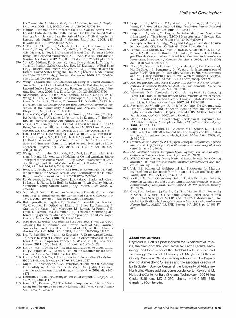
Eta-Community Multiscale Air Quality Modeling System; J. Geophys.Res. Atmos. 2008, 113, D02303; doi: 10.1029/2007jd008580.

194. Mathur, R. Estimating the Impact of the 2004 Alaskan Forest Fires onEpisodic Particulate Matter Pollution over the Eastern United Statesthrough Assimilation of Satellite-Derived Aerosol Optical Depths in aRegional Air Quality Model; J. Geophys. Res. Atmos. 2008, 113,D17302; doi: 10.1029/2007jd009767.

195. McKeen, S.; Chung, S.H.; Wilczak, J.; Grell, G.; Djalalova, I.; Peck-ham, S.; Gong, W.; Bouchet, V.; Moffet, R.; Tang, Y.; Carmichael,G.R.; Mathur, R.; Yu, S. Evaluation of Several PM2.5 Forecast ModelsUsing Data Collected during the ICARTT/NEAQS 2004 Field Study; J.Geophys. Res. Atmos. 2007, 112, D10s20; doi: 10.1029/2006jd007608.

196. Yu, S.C.; Mathur, R.; Schere, K.; Kang, D.W.; Pleim, J.; Young, J.;Tong, D.; Pouliot, G.; McKeen, S.A.; Rao, S.T. Evaluation of Real-TimePM2.5 Forecasts and Process Analysis for PM2.5 Formation over theEastern United States Using the Eta-CMAQ Forecast Model duringthe 2004 ICARTT Study; J. Geophys. Res. Atmos. 2008, 113, D06204;doi: 10.1029/2007jd009226.

197. Wang, J.; Christopher, S.A. Mesoscale Modeling of Central AmericanSmoke Transport to the United States: 2. Smoke Radiative Impact onRegional Surface Energy Budget and Boundary Layer Evolution; J. Geo-phys. Res. Atmos. 2006, 111, D14S92; doi: 10.1029/2005jd006720.

198. Newchurch, M.A.B.; Khan, M.S.; Koshak, B.; Nair, U.S.; Fuller, K.;Wang, L.; Park, Y.; Williams, R.; Christopher, S.; Kim, J.; Liu, X.;Byun, D.; Pierce, B.; Chance, K.; Kurosu, T.P.; McMillan, W.W. Im-provements in Air-Quality Forecasts from Satellite Observations. Pre-sented at the Community Modeling and Analysis Conference,Chapel Hill, NC, October 6–8, 2008.

199. Justice, C.O.; Giglio, L.; Korontzi, S.; Owens, J.; Morisette, J.T.; Roy,D.; Descloitres, J.; Alleaume, S.; Petitcolin, F.; Kaufman, Y. The MO-DIS Fire Products; Remote Sens. Environ. 2002, 83, 244-262.

200. Zhang, X.Y.; Kondragunta, S. Estimating Forest Biomass in the USAUsing Generalized Allometric Models and MODIS Land Products;Geophys. Res. Lett. 2006, 33, L09402; doi: 10.1029/2006gl025879.

201. Reid, J.S.; Prins, E.M.; Westphal, D.L.; Schmidt, C.C.; Richardson,K.A.; Christopher, S.A.; Eck, T.F.; Reid, E.A., Curtis, C.A.; Hoffman,J.P. Real-Time Monitoring of South American Smoke Particle Emis-sions and Transport Using a Coupled Remote Sensing/Box-ModelApproach; Geophys. Res. Lett. 2004, 31, L06107; doi: 10.1029/2003gl018845.

202. Wang, J.; Christopher, S.A.; Nair, U.S.; Reid, J.S.; Prins, E.M.; Szyk-man, J.; Hand, J.L. Mesoscale Modeling of Central American SmokeTransport to the United States: 1. “Top-Down” Assessment of Emis-sion Strength and Diurnal Variation Impacts; J. Geophys. Res. Atmos.2006, 111, doi: 10.1029/2005jd006416.

203. Stein, A.F.; Rolph, G.D.; Draxler, R.R.; Stunder, B.; Ruminski, M. Verifi-cation of the NOAA Smoke Forecast: Model Sensitivity to the InjectionHeight; Weather Forecast. doi: 10.1175/2008WAF2222166.1.

204. Kondragunta, S.; Lee, P.; McQueen, J.; Kittaka, C.; Prados, A.I.; Ciren,P.; Laszlo, I.; Pierce, R.B.; Hoff, R.; Szykman, J.J. Air Quality ForecastVerification Using Satellite Data; J. Appl. Meteor. Clim. 2008, 47,425-442.

205. Schmidt, H., Martin, D. Adjoint Sensitivity of Episodic Ozone in theParis Area to Emissions on the Continental Scale; J. Geophys. Res.Atmos. 2003, 108, 8561; doi: 10.1029/2001jd001583.

206. Hollingsworth, A.; Engelen, R.J.; Textor, C.; Benedetti, A.; Boucher,O.; Chevallier, F.; Dethof, A.; Elbern, H.; Eskes, H.; Flemming, J.;Granier, C.; Kaiser, J.W.; Morcrette, J.J.; Rayner, P.; Peuch, V.H.;Rouil, L.; Schultz, M.G.; Simmons, A.J. Toward a Monitoring andForecasting System for Atmospheric Composition: the GEMS Project;Bull. Am. Meteor. Soc. 2008, 89, 1147-1164.

207. Stavrakou, T.; Muller, J.F.; Boersma, K.F.; De Smedt, I.; van der A, R.J.;Assessing the Distribution and Growth Rates of NOx EmissionSources by Inverting a 10-Year Record of NO2 Satellite Columns;Geophys. Res. Lett. 2008, 35, L10801; doi: 10.1029/2008gl033521.

208. Liu, Y.; Franklin, M.; Kahn, R.; Koutrakis, P. Using Aerosol OpticalThickness to Predict Ground-Level PM2.5 Concentrations in the St.Louis Area: a Comparison between MISR and MODIS; Rem. Sens.Environ. 2007, 107, 33-44; doi: 10.1016/j.rse.2006.05.022.

209. Rossow, W.B.; Duenas, E.N. The International Satellite Cloud Clima-tology Project (ISCCP) Website—an Online Resource for Research;Bull. Am. Meteor. Soc. 2004, 85, 167-172.

210. Rossow, W.B.; Schiffer, R.A. Advances in Understanding Clouds fromISCCP; Bull. Am. Meteor. Soc. 1999, 80, 2261-2287.

211. Gupta, P.; Christopher, S.A. An Evaluation of Terra-MODIS Samplingfor Monthly and Annual Particulate Matter Air Quality Assessmentover the Southeastern United States; Atmos. Environ. 2008, 42, 6465-6471.

212. Kaufman, Y. J. Satellite Sensing of Aerosol Absorption; J. Geophys. Res.1987, 92, 4307-4317.

213. Fraser, R.S.; Kaufman, Y.J. The Relative Importance of Aerosol Scat-tering and Absorption in Remote Sensing; IEEE Trans. Geosci. RemoteSens. 1985, 5, 625-633.

214. Lyapustin, A.; Williams, D.L.; Markham, B.; Irons, J.; Holben, B.;Wang, Y. A Method for Unbiased High-Resolution Aerosol Retrievalfrom Landsat; J. Atmos. Sci. 2004, 61, 1233-1244.

215. Lyapustin, A.; Wang, Y.; Frey, R. An Automatic Cloud Mask Algo-rithm based on Time Series of MODIS Measurements; J. Geophys. Res.Atmos. 2008, 113, D16207; doi: 10.1029/2007jd009641.

216. Test Specifications for PM10, PM2.5 and PM10–2.5 Candidate Equiva-lent Methods. CFR, Part 53, Title 40, 2006, Appendix C-4.

217. Lamsal, L.N.; Martin, R.V.; van Donkelaar, A.; Steinbacher, M.; Ce-larier, E.A.; Bucsela, E.; Dunlea, E.J.; Pinto, J.P. Ground-Level Nitro-gen Dioxide Concentrations Inferred from the Satellite-Borne OzoneMonitoring Instrument; J. Geophys. Res. Atmos. 2008, 113, D16308;doi: 10.1029/2007jd009235.

218. Blond, N.; Boersma, K.F.; Eskes, H.J.; van der A, R.J.; Van Roozendael,M.; De Smedt, I.; Bergametti, G.; Vautard, R. Intercomparison ofSCIAMACHY Nitrogen Dioxide Observations, in Situ Measurementsand Air Quality Modeling Results over Western Europe; J. Geophys.Res. Atmos. 2007, 112, D10311; doi: 10.1029/2006jd007277.

219. Risk and Exposure Assessment to Support the Review of the NO2 PrimaryNational Ambient Air Quality Standard; U.S. Environmental ProtectionAgency: Research Triangle Park, NC, 2008.

220. Whiteman, D.N.; Veselovskii, I.; Cadirola, M.; Rush, K.; Comer, J.;Potter, J.R.; Tola, R. Demonstration Measurements of Water Vapor,Cirrus Clouds, and Carbon Dioxide Using a High-Performance Ra-man Lidar; J. Atmos. Oceanic Tech. 2007, 24, 1377-1388.

221. Ansmann, A.; Wandinger, U.; Le Rille, O.; Lajas, D.; Straume, A.G.Particle Backscatter and Extinction Profiling with the SpaceborneHigh-Spectral-Resolution Doppler Lidar ALADIN: Methodology andSimulations; Appl. Opt. 2007, 46, 6606-6622.

222. Marini, A.E. ATLID: the Technology Development Programme forESA’s Satellite-Borne Atmospheric Lidar; ESA Bull. Eur. Space Agency1998, 95, 113-118.

223. Schmit, T.J.; Li, J.; Gurka, J.J.; Goldberg, M.D.; Schrab, K.J.; Li, J.L.;Feltz, W.F. The GOES-R Advanced Baseline Imager and the Contin-uation of Current Sounder Products; J. Appl. Meteor. Clim. 2008, 47,2696-2711.

224. Overview of the “Ibuki” (GOSAT); Japan Aerospace Exploration Agency;available at http://www.jaxa.jp/countdown/f15/overview/ibuki_e.html (ac-cessed January 31, 2009).

225. ESA Satellite Missions; European Space Agency; available at http://earth.esa.int/missions/ (available at January 31, 2009).

226. NSSDC Master Catalog Search; National Space Science Data Center;available at http://nssdc.gsfc.nasa.gov/nmc/spacecraftSearch.doc (ac-cessed January 31, 2009).

227. Volz, F.E. Economical Multispectral Sun Photometer for Measure-ments of Aerosol Extinction from 0.44 �m to 1.6 �m and PrecipitableWater; Appl. Opt. 1974, 13, 1732-1733.

228. Krotkov, N. Earth Observatory: Sulfur Dioxide Emissions, Bulgaria;National Aeronautics and Space Administration; available at http://earthobservatory.nasa.gov/IOTD/view.php?id�36790 (accessed January31, 2009).

229. Chu, D.A.; Szykman, J.; Kittaka, C.; Chin, M.; Liu, H.-C.; Remer, L.;Al-Saadi, J.; Winker, D. Developing Aerosol Height Product fromMODIS and Synergy of MODIS and CALIPSO Measurements forGlobal Application. In Atmospheric Remote Sensing for Air Pollution andHuman Health, IGARSS ’08, SPIE: Boston, MA, 2008; pp IV-303–IV-306.

About the AuthorsRaymond M. Hoff is a professor with the Department of Phys-ics, the director of the Joint Center for Earth Systems Tech-nology, and the director of the Goddard Earth Sciences andTechnology Center at University of Maryland/ BaltimoreCounty. Sundar A. Christopher is a professor with the Depart-ment of Atmospheric Sciences and the associate director ofEarth System Science Center at the University of Alabama–Huntsville. Please address correspondence to: Raymond M.Hoff, Joint Center for Earth Systems Technology, 1000 HilltopCircle, Baltimore, MD 21250; phone: �1-410-455-1610;e-mail: [email protected].



remote sensing of particulate pollution from space: … · remote sensing of particulate pollution...

Documents