| T H E A U S T R A L I A N N A T I O N A L U N I V E R S I T Y

Crawford School of Public Policy

Centre for Climate Economics & Policy

Economic growth and global particulate pollution concentrations

CCEP Working Paper 1604 Feb 2016

David I. Stern Crawford School of Public Policy, The Australian National University Jeremy van Dijk Australian Bureau of Agricultural and Resource Economics and Sciences, Australia

Abstract Though the environmental Kuznets curve (EKC) was originally developed to model the ambient concentrations of pollutants, most subsequent applications focused on pollution emissions. Yet, previous research suggests that it is more likely that economic growth could eventually reduce the concentrations of local pollutants than emissions. We examine the role of income, convergence, and time related factors in explaining changes in PM2.5 pollution in a global panel of 158 countries between 1990 and 2010. We find that economic growth has positive but relatively small effects, time effects are also small but larger in wealthier and formerly centrally planned economies, and, for our main dataset, convergence effects are small and not statistically significant. There is no in-sample income turning point for regressions that include both the convergence variables and a set of control variables.

| T H E A U S T R A L I A N N A T I O N A L U N I V E R S I T Y

Keywords:

Air pollution; economic growth; environmental Kuznets curve

JEL Classification:

O44, Q53, Q56

Suggested Citation:

Stern, D.I. and van Dijk, J. (2016), Economic growth and global particulate pollution concentrations, CCEP Working Paper 1604, Feb 2016. Crawford School of Public Policy, The Australian National University.

Address for Correspondence:

David I. Stern Professor Crawford School of Public Policy The Australian National University 132 Lennox Crossing Acton ACT 2601 Australia Tel: +61 2 61250176 Email: david.stern@anu.edu.au

The Crawford School of Public Policy is the Australian National University’s public policy school, serving

and influencing Australia, Asia and the Pacific through advanced policy research, graduate and executive

education, and policy impact.

The Centre for Climate Economics & Policy is an organized research unit at the Crawford School of Public

Policy, The Australian National University. The working paper series is intended to facilitate academic and

policy discussion, and the views expressed in working papers are those of the authors. Contact for the

Centre: Dr Frank Jotzo, frank.jotzo@anu.edu.au

Economic Growth and Global Particulate Pollution

Concentrations

David I. Stern

Crawford School of Public Policy, The Australian National University, 132 Lennox Crossing,

Acton, ACT 2601, Australia. david.stern@anu.edu.au

Jeremy van Dijk

Australian Bureau of Agricultural and Resource Economics and Sciences, Canberra, ACT 2601,

Australia.

29 February 2016

Abstract

Though the environmental Kuznets curve (EKC) was originally developed to model the

ambient concentrations of pollutants, most subsequent applications focused on pollution

emissions. Yet, previous research suggests that it is more likely that economic growth could

eventually reduce the concentrations of local pollutants than emissions. We examine the role

of income, convergence, and time related factors in explaining changes in PM2.5 pollution in a

global panel of 158 countries between 1990 and 2010. We find that economic growth has

positive but relatively small effects, time effects are also small but larger in wealthier and

formerly centrally planned economies, and, for our main dataset, convergence effects are small

and not statistically significant. There is no in-sample income turning point for regressions that

include both the convergence variables and a set of control variables.

Keywords: Air pollution, economic growth, environmental Kuznets curve

JEL Codes: O44, Q53, Q56

Acknowledgements: We thank Rohan Best, Zsuzsanna Csereklyei, Paul Burke, Astrid Kander,

and Luis Sanchez for helpful comments.

1. Introduction

Particulate pollution, especially PM2.5, is thought to be the form of pollution with the most

serious human health impacts (WHO, 2013). It is estimated that PM2.5 exposure causes 3.1

million deaths a year, globally, and any level above zero is deemed unsafe, i.e. there is no

threshold above zero below which negative health effects do not occur (WHO 2013). Black

carbon is an important fraction of PM2.5 pollution (Vidanoja et al., 2002) that may contribute

significantly to anthropogenic radiative forcing (Bond et al., 2013) and, therefore, there may

be significant co-benefits to reducing its concentration (Victor et al., 2015). Though the

environmental Kuznets curve (EKC) was originally developed to model the ambient

concentrations of pollutants, most subsequent applications focused on pollution emissions. Yet,

it would seem more likely that economic growth could eventually reduce the concentrations of

local pollutants than emissions (Selden and Song, 1994; Stern et al., 1996). Here, we examine

the role of income, convergence, and time related factors in explaining changes in PM2.5

particulate pollution in a global panel of countries between 1990 and 2010. We use a recently

developed model that integrates the EKC and convergence approaches. We find that economic

growth has positive but relatively small effects, time effects are also small but larger in

wealthier and formerly centrally planned economies, and, for our main dataset, convergence

effects are small and not statistically significant. The surprising finding is that there isn’t an

EKC even for local pollution concentrations, though the effects of economic growth are much

smaller than they are for emissions of carbon and sulfur dioxide.

The environmental Kuznets curve (EKC) has been the dominant approach among economists

to modeling ambient pollution concentrations and aggregate emissions since Grossman and

Krueger (1991) introduced it a quarter of a century ago. The EKC is characterized by an income

turning point – the level of GDP per capita after which economic growth reduces rather than

increases environmental impacts. Though the EKC was originally developed to model the

ambient concentrations of pollutants, most subsequent applications have focused on pollution

emissions and in particular carbon dioxide and sulfur dioxide (Carson, 2010). Recent studies

using global data sets find that, in fact, income has a monotonic positive effect on the emissions

of both these pollutants (Wagner, 2008; Vollebergh et al., 2009; Stern, 2010; Anjum et al.,

2014).

Both Selden and Song (1994) and Stern et al. (1996) noted that ambient concentrations of

pollutants were likely to fall before emissions did. Stern (2004) suggests that this may be due

to both the decline in urban population densities and the decentralization of industry that tend

to accompany economic growth. Furthermore, actions through which governments can try to

reduce local air pollution include moving industry outside of populated areas and building taller

smokestacks. The latter reduced urban air pollution in developed countries in the 20th Century

at the expense of increasing acid rain in neighboring countries and the formation of sulfate

aerosols (Wigley and Raper, 1992). Additionally, pollutants with severe and obvious human

health impacts such as particulates are more likely to be controlled earlier than pollutants with

less obvious impacts such as carbon dioxide (Shafik, 1994). Despite this, relatively little recent

research has attempted to apply the EKC to pollution concentrations rather than emissions.

More recently, it has become popular to model the evolution of emissions using convergence

approaches. Pettersson et al. (2013) provide a review of the literature on convergence of carbon

emissions. There are three main approaches to testing for convergence: sigma convergence,

which tests whether the dispersion of the variable in question declines over time using either

just its variance or its full distribution (e.g. Ezcurra, 2007); stochastic convergence, which tests

whether the time series for different countries cointegrate; and beta convergence, which tests

whether the growth rate of a variable is negatively correlated to the initial level. We are not

aware of attempts to test for convergence in pollution concentrations rather than emissions.

Yet, it seems reasonable that high concentrations of pollution would encourage defensive

action to reduce that pollution (Ordás Criado et al., 2011).

Sanchez and Stern (2016) propose a regression model that nests both the EKC and beta

convergence models, which can be seen as an extension of Ordás Criado et al.’s (2011) model

to also include the EKC effect. The model allows us to test the contributions of economic

growth, convergence, and time effects to the evolution of pollution.

Our main results use population-weighted estimates of national average concentrations of

PM2.5 pollution from the World Bank Development Indicators. These data are based on Brauer

et al. (2016), who used satellite observations of aerosol optical depth, pollution emissions data

to obtain estimates, which were then regressed on the available ground-based observations.

The resulting coefficients were used to project calibrated PM2.5 for all parts of the world. To

check robustness we also use the Environmental Performance Index dataset. These data are

based on Boys et al. (2014) and van Donkelaar et al. (2015). Neither of these latter studies uses

ground-based ambient observations in deriving their estimates. More details are provided in

the Appendix. Because both these datasets are weighted by population exposure, they most

reflect the concentrations of these pollutants in densely populated areas such as cities. Thus,

though obviously particulates travel between cities and countries in the wind, we are capturing

local pollution to a large extent with this data set.

The next section of the paper reviews previous research on modeling particulate pollution

concentrations. The third section presents our modeling approach, the fourth our data, and the

fifth our results. The sixth section presents our conclusions.

2. Previous Research

Grossman and Krueger (1991) estimated the first EKC models as part of a study of the potential

environmental impacts of NAFTA. They estimated EKCs for SO2, dark matter (fine smoke),

and suspended particles (SPM) using the GEMS dataset. This dataset is a panel of ambient

measurements from a number of locations in cities around the world. Each regression involved

a cubic function in levels (not logarithms) of PPP (Purchasing Power Parity adjusted) per capita

GDP, various site-related variables, a time trend, and a trade intensity variable. The turning

points for SO2 and dark matter were at around $4,000-5,000 while the concentration of

suspended particles appeared to decline even at low income levels. However, Harbaugh et al.

(2002) re-examined an updated version of Grossman and Krueger’s data. They found that the

locations of the turning points for the various pollutants, as well as even their existence, were

sensitive both to variations in the data sampled and to reasonable changes in the econometric

specification.

Shafik’s (1994) study was particularly influential, as its results were used in the 1992 World

Development Report. Shafik estimated EKCs for ten different indicators using three different

functional forms. She found that local air pollutant concentrations conformed to the EKC

hypothesis with turning points between $3,000 and $4,000. Selden and Song (1994) estimated

EKCs for four emissions series: SO2, NOx, SPM, and CO. The estimated turning points were

all very high compared to the two earlier studies. For the fixed effects version of their model

they are (in 1990 US dollars): SO2, $10,391; NOx, $13,383; SPM, $12,275; and CO, $7,114.

This showed that the turning points for emissions were likely to be higher than for ambient

concentrations.

There has been little recent EKC research on particulate pollution. Keene and Deller (2015)

recently published an EKC analysis of PM2.5 concentrations for a cross-section of U.S.

counties. The model includes state dummies and various control variables and they use OLS

and spatial econometric estimators. They find that the peak of the EKC occurs at between

US$24,000 and US$25,500, depending on the estimator used.

Some recent research focuses on Chinese cities. Brajer et al. (2011) investigate ambient

concentrations of SO2, NO2, and total suspended particulates and also construct indices of total

air pollution using the Nemerow approach and an alternative proposed by Khanna (2000). Their

data cover the period 1990-2006 for 139 Chinese cities. They use a logarithmic EKC model

with city random effects and a linear time trend with the addition of population density variable.

Using the quadratic EKC model, they estimate the turning point for TSP at RMB 3,794, not

controlling for population density, and at RMB 6,253, controlling for population density.

However, the regression coefficient of the cube of log income in a cubic EKC model is

statistically significantly greater than zero. This second turning point occurs around RMB 125k.

Hao and Liu (2016) estimate EKC models for PM2.5 concentrations and the official Air

Quality Index in a cross-section of 73 Chinese cities in 2013. They find an inverted U shape

curve with highly significant parameter estimates for OLS and SEM estimates, with turning

points of RMB 9k to 40k and PM2.5, respectively.

3. Models

Our model combines the three main approaches in the literature and includes other possible

drivers of change in concentrations by nesting these existing specifications in a single

regression equation:

�̂�𝑖 = 𝛼 + 𝛽1�̂�𝑖 + 𝛽2𝐺𝑖0�̂�𝑖 + 𝛽3𝐺𝑖0 + 𝛽4𝐶𝑖0 + ∑ 𝜓𝑗

𝑗

𝑋𝑗𝑖 + 𝜀𝑖

where i indexes countries, 0 indicates the initial year of the sample, and 𝜀𝑖 is a random error

term. �̂�𝑖 and �̂�𝑖 are the long-run growth rates of concentrations and income, respectively. 𝐺𝑖0

is the log of income per capita in the first year in the sample in each country and 𝐶𝑖0 is the log

of concentrations in the initial year. X is a vector of additional explanatory or “control”

variables. We also estimate models that exclude the control variables, and which exclude the

control and levels variables, 𝐺𝑖0 and 𝐶𝑖0. The latter model is analogous to the traditional EKC

model, but estimated using differences rather than levels of the variables.

We compute long-run growth rates using: �̂�𝑖 = (𝑌𝑖𝑇 − 𝑌𝑖0)/𝑇, where Y is the logarithm of

concentrations or per capita income and T+1 is the number of years in the sample. By

formulating our model in long-run growth rates we avoid most of the econometric problems

troubling the existing literature on the environmental Kuznets curve, which are discussed in

several recent contributions (Wagner, 2008, 2015; Vollebergh et al., 2009; Stern, 2010;

Anjum et al., 2014).

We subtract the means of all the continuous levels variables (as opposed to growth rates or

dummy variables) prior to estimation. Therefore, the first term on the RHS of the equation, ,

is the growth rate of concentrations when there is no economic growth and all the other

continuous levels variables are at their sample means. This can, therefore, be interpreted as

the average time effect. 𝛽1is an estimate of the income-concentrations elasticity at the

sample mean. The third term tests for the EKC effect. If 𝛽2 is statistically significantly

negative and 𝛽1 is positive, then there is a level of income after which concentrations reduce

with growth. We can find the EKC turning point, , by estimating the regression without

demeaning 𝐺𝑖0 prior to computing 𝐺𝑖0�̂�𝑖 and then computing 𝜇 = 𝑒𝑥𝑝(−𝛽1/𝛽2) using the

estimated coefficients. If this turning point is within the sample range of income then there is

an environmental Kuznets curve. If 𝛽2 is negative, but the turning point is out of sample, we

can still say that there is an EKC effect so that growth has a reduced effect on concentrations

at higher income levels.

The fourth term tests whether concentrations change at a different rate in richer countries in

the absence of growth and the fifth term is intended to model convergence by allowing us to

test for convergence in concentrations using the beta convergence approach. If 𝛽4 < 0, t

concentrations converge across countries so that concentrations growth is slower in countries

that commence the period with higher pollution concentrations and vice versa.

A wide variety of “control variables” have been considered in the EKC literature. Some of

these are genuinely exogenous or predetermined, whereas others are variables that typically

change in the course of economic development and might be seen as factors through which

the development process drives concentrations changes. Examples of the latter are

democracy, free press, good governance, lack of corruption, or industrial structure. We are

interested in testing the overall effect of income and economic growth on pollution growth

and so we only include variables that are pre-determined or exogenous to the development

process and found in previous research to be potentially relevant.

Stern (2005) first noted that English speaking OECD countries seemed to abate sulfur

emissions less and Germanic and Scandinavian countries more. Stern (2012) related this to

differences in legal origins (La Porta et al., 2008) and found that energy intensity was lower

in non-English legal origin countries, ceteris paribus. Fredriksson and Wollscheid (2015)

present evidence that legal origin has a significant effect on environmental policy. Here, we

include dummies for French and German legal origin. We also control for whether a country

was a formerly centrally planned country using a dummy variable. We expect that market

reform would reduce the level of pollution, ceteris paribus.

We also control for the effect of climate, by using historical country averages of temperatures

over the three summer months and the three winter months, annual precipitation, and average

elevation above sea level. The latter two variables are converted to logarithms. We also

control for landlocked status, as landlocked countries are less likely to have the higher wind

speeds seen in coastal regions. Indonesia, Singapore and Malaysia experienced very high

levels of pollution in 1990 associated with the periodic haze episodes due to forest fires in the

region (Osterman and Brauer, 2001). We add a dummy for these three countries. Finally, we

include the average of the log of population density, which might be expected to increase the

concentration of pollution, ceteris paribus. Also, the higher population is, the more people

will be exposed to pollution and the more likely that action might be taken (Ordás Criado et

al., 2011).

When observations on variables are aggregated into regions – here countries - of different

sizes, it is likely that much of the local variation across individual locations is cancelled out

in the larger regions while more idiosyncratic variation remains in smaller regions. This

means that the error terms in a regression using such aggregated data are likely to be

heteroskedastic with the error variance proportional to the district size (Maddala, 1977; Stern,

1994). As our data consists of population-weighted concentrations by country, the

appropriate measure of region size is population. To address this grouping heteroskedasticity

we estimate the models using weighted least squares, where the weights are the square root of

population, and heteroskedasticity-robust standard errors. Using weighted least squares

(WLS) can result in large efficiency gains over using ordinary least squares (OLS) even when

the model for reweighting the data is misspecified. But in case there is misspecification,

heteroskedasticity robust standard errors should be used to ensure correct inference (Romano

and Wolf, 2014). We measure goodness of fit using Buse’s (1973) R-squared, weighting the

squared deviations by population.

We assume that the explanatory variables in our regressions are exogenous. Clearly, there can

be no reverse causality from growth rates to initial values. There may potentially be apparent

feedback from the growth rate of concentrations to the growth rate of income. This is because

pollution growth may be correlated with the growth of energy use and energy use contributes

to economic growth. Csereklyei and Stern (2015) argue that this bias will be fairly small even

when the dependent variable is energy use and so the estimated energy-income elasticity will

not be far from the causal effect size of an exogenous change in income. Here, the potential

bias should be smaller still. Omitted variables bias is an important issue as there are many

variables that may be correlated with the level of GDP or GDP growth, and which may help

explain concentrations growth. Our differenced approach should help reduce this bias

(Angrist and Pischke, 2010). Finally, measurement error is a significant issue in the

estimation of GDP and pollution concentrations. Obviously there are significant uncertainties

in the concentrations data, which are modeled based on satellite and ground-based

measurements. Measurement error is likely greater for some of the smaller economies.

Weighted least squares can, therefore, help reduce the effects of this measurement error. A

common approach to dealing with reverse causality, omitted variables bias, and measurement

error is to use instrumental variables. However, it is hard to find plausible instrumental

variables in the macro-economic context (Bazzi and Clemens, 2013).

4. Data

Details of the data sources are presented in the Appendix.

Table 1 presents some descriptive statistics for our variables. These are the variables sourced

from the World Bank Development Indicators used in the main analysis. The PM2.5

concentration exposure level in 1990 is mostly above the WHO guideline of 10 μg/m3 with a

mean and median of 18-19 μg/m3. The range of observations is quite large, from below 1 μg/m3

to over 76 μg/m3 in Mauritania. In 1990, Singapore had the second highest level of PM2.5 at

49.8 μg/m3. But this was anomalously high as discussed above. As of 2005, 89% of the world’s

population was exposed to annual mean PM2.5 concentration levels higher than the WHO

concentration guideline of 10 μg/m3, while approximately two thirds of countries were in this

category (Brauer et al., 2012). This difference is due to the large populations in East and South

Asia, which have high PM2.5 concentration levels. In the base year of the study, 1990, 67% of

countries in the sample had exposure levels higher than the WHO recommendation.

The level of initial per capita GDP has a wide range from $365 to $114,519 in constant 2011

PPP Dollars. While mean income per capita is $11,895, the median value is only half the

mean, at $6,440. The descriptive statistics for the continuous control variables exhibit the

wide range that would be expected in a globally representative sample.

Table 1 also presents the annual growth rates of income per capita and pollution. GDP per

capita grows at an average rate of 1.76% p.a. over the period 1990 to 2010. The median is

only 0.13 percentage points lower. The income growth rates are mostly positive, however 24

countries had negative growth over the period. There are two outliers with GDP per capita

growth rates larger than 9% p.a. – China and Equatorial Guinea. Compared to GDP growth

rates, the growth rates of pollution exposure are mostly modest. The mean rate of decline was

-0.35% p.a., and the median 0.17% p.a. 78 countries had positive growth in PM2.5 exposure

over the period. The highest growth was in Micronesia, averaging 6.5% p.a., while the most

rapid decrease was observed in Singapore averaging -6.9% p.a. But in both these countries

there was a large change in one decade but not the other. In fact, while the mean annual rate

of decline of PM2.5 in the 1990s was 0.88%, PM2.5 concentrations on average increased in the

following decade with an average annual growth rate of 0.18%.

Figure 1 presents the data in growth rates form. There would not be much point in presenting

the actual concentrations of pollution as the mean levels are swept out when growth rates are

computed and much of the variation in levels reflects idiosyncrasies of geography. The size of

the bubbles is proportional to population in 1990, which is used to weight the observations in

the regression analysis. The large circle to the right is, of course, China, with India to its left.

The USA is the largest circle among the countries with negative pollution growth rates.

Indonesia is to its lower right. As we can see, both pollution and GDP per capita rose quite

strongly in the World’s two most populous countries. This and the negative pollution growth

rates in many of the countries with moderate growth suggest that economic growth should have

significant effects on pollution growth. OLS estimates are likely to be influenced by some of

the small outlier countries such as Equatorial Guinea on the far right of the Figure, which is

mitigated by using WLS to estimate our main models.

5. Results

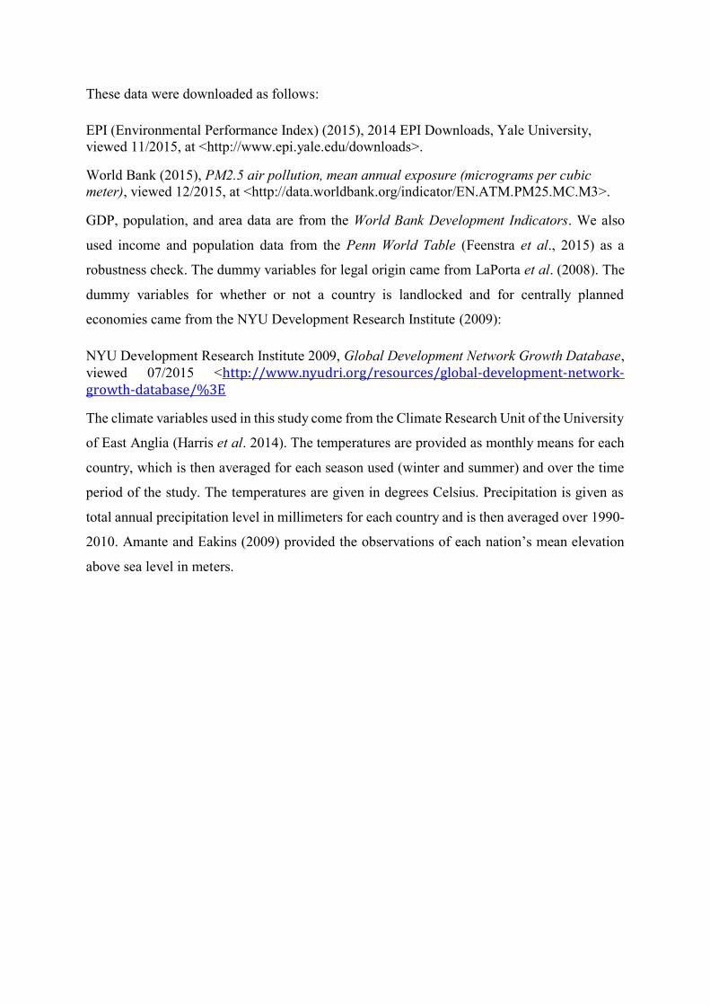
Table 2 presents the main results, which use World Bank pollution and GDP data. The simple

EKC model has a turning point at $3,336, which is statistically significantly different from zero.

The concentrations-GDP elasticity at the sample mean is -0.18, though not very precisely

estimated. It is negative because the income turning point is below the mean income in the

sample. The time effect is small and not statistically significant. These results would seem to

strongly support the environmental Kuznets curve story and the hypothesis that the income

turning point is lower for concentrations of local pollutants than it is for emissions of pollutants

such as sulfur dioxide. The second column adds the two initial levels terms. The EKC turning

point is now much higher, but very imprecisely estimated. In addition, the concentrations-GDP

elasticity at the sample mean is now positive. As expected, the coefficient of initial pollution

is negative indicating beta convergence. The coefficient of initial income is also negative and

very significant. This implies that concentrations fall faster in richer countries, ceteris paribus.

When we add the control variables, the concentrations-income elasticity rises to 0.21 at the

sample mean and is highly significant and the interaction term, which tests the EKC hypothesis,

is significant at the 10% level. However the EKC turning point rises further to $66,728 so that

the EKC is effectively monotonic. The effects of the initial levels are reduced in strength and

statistical significance. Of the control variables, concentrations rise faster (or fall slower) in

countries with higher summer, lower winter temperatures, and higher precipitation and rise

slower (or fall faster) in formerly centrally planned countries as we would expect. Of these, the

effect of precipitation is unexpected, as higher precipitation would be expected to clear the air.

Many of the countries where concentrations fell strongly are in Europe and have moderate

levels of rainfall around 500-1000mm, while many of the countries where concentrations rose

most strongly happen to be in areas of heavy rainfall in the tropics. This effect might be related,

therefore, to deforestation. The Malaysia, Singapore, and Indonesia dummy has a highly

significant and negative effect on concentrations growth.

Results are, therefore, similar to those found by Anjum et al. (2014) for sulfur and carbon

emissions, but the effect of economic growth is far smaller and even smaller than that for non-

industrial greenhouse gas emissions (Sanchez and Stern, 2016). The convergence effect is also

weaker than for industry related emissions. When we control for other relevant variables there

is not even an environmental Kuznets curve for particulate concentrations.

We also present results for the following variations, to test robustness to different data sources,

time periods, and estimation methods:

1. Use OLS instead of WLS.

2. Split the data used in Table 2 into two time periods – 1990-2000 and 2000-2010.

3. Use income from the Penn World Table instead of the World Bank.

4. Use pollution data from EPI instead of the World Bank.

We report these results for the full model in Table 3. Looking first at the OLS results, the main

differences are that both income terms are much smaller and not significant, the convergence

effect is highly significant, the effects of elevation and legal origin are larger and much more

significant, and the effects of centrally planned status are smaller. On the other hand, these

results are not dramatically different from the WLS results. One of the advantages of the latter

are that they are much more robust to changes in the sample of countries, as we go to the

remaining analyses.

The results from splitting the sample into 1990-2000 and 2000-2010 periods in the Columns 2

and 3 differ in somewhat expected ways from the 1990-2010 estimates in Table 2. Again the

EKC is effectively monotonic but in one case there is an out of sample turning point and in the

other a minimum near zero. The income elasticity at the sample mean is higher in the second

period. One reason for this is that income increases from the first to second period. The effects

of central planning and the Malaysia, Singapore, and Indonesia dummy decrease in the second

period, as we would expect. Unexpected results are that elevation has a positive effect in the

first period and precipitation only in the second period. Though these results show a stronger

effect of growth in the second period, the effect of growth on concentrations is still relatively

small compared to estimates for emissions of other pollutants related to industrial activity but

about the same as for non-industrial greenhouse gas emissions, which are primarily from land-

use change (Sanchez and Stern, 2016).

Results using income data from the Penn World Table in Column 4 are very similar to those

for the World Bank income data in Table 2 but there are more statistically significant

coefficients including for elevation, landlockedness, and French legal origin. However, central

planning is not statistically significant here.

The results in the final column using EPI data for 2000-2010 and World Bank income data are

similar in some respects to the 2000-2010 World Bank pollution data estimates in Column 3.

The concentrations-income elasticity is 0.38 and very statistically significant. In contrast to the

World Bank pollution data, the convergence effect is quite large and statistically significant.

Also, landlockedness and French legal origin now have significant negative effects and

population density a significant positive effect.

6. Conclusions

The evidence presented in this article shows that economic growth has positive though

relatively small effects on the growth in PM2.5 concentrations. For our models that include

convergence terms and control variables there is no sign of in-sample income turning point.

However, when we estimate a model analogous to the classic EKC model we find a turning

point of around $3,000 per capita. Our results suggest that prior studies that find a relatively

low income turning point for the environmental Kuznets curve for particulate concentrations

(e.g. Grossman and Krueger, 1991; Shafik, 1994; Brajer et al., 2011; Hao and Liu, 2016) suffer

from omitted variables bias. Our results are more similar to Keene and Deller (2015) who found

a much higher, but still in-sample, turning point for U.S. counties.

On the other hand, the negative time effect is stronger in richer countries, but this is unrelated

to increases in income. What is clear is that this behavior is very different from emissions of

sulfur or industrial greenhouse gases where typically a strong positive effect of economic

growth is found at the sample mean income (Anjum et al., 2014; Sanchez and Stern, 2016).

That there is not even an EKC for particulate pollution, which is a classic example of a mostly

local pollutant that impacts human health, casts further doubt on the general usefulness of the

EKC model.

References

Amante, C. and Eakins, B. W. 2009. Etopo1 1 Arc-Minute Global Relief Model: Procedures,

Data Sources and Analysis, NOAA Technical Memorandum NESDIS NGDC-24, National

Geophysical Data Center, NOAA.

Angrist, J. D. and J.-S. Pischke. 2010. The credibility revolution in empirical economics: how

better research design is taking the con out of econometrics. Journal of Economic

Perspectives, 24(2): 3-30.

Anjum Z., P. J. Burke, R. Gerlagh, and D. I. Stern. 2014. Modeling the emissions-income

relationship using long-run growth rates, CCEP Working Papers 1403.

Bazzi, S. and M. A. Clemens. 2013. Blunt instruments: Avoiding common pitfalls in

identifying the causes of economic growth. American Economic Journal: Macroeconomics

5(2): 152–186.

Bond, T. C., S. J. Doherty, D. W. Fahey, P. M. Forster, T. Berntsen, B. J. DeAngelo, M. G.

Flanner, S. Ghan, B. Kärcher, D. Koch, S. Kinne, Y. Kondo, P. K. Quinn, M. C. Sarofim, M.

G. Schultz, M. Schulz, C. Venkataraman, H. Zhang, S. Zhang, N. Bellouin, S. K. Guttikunda,

P. K. Hopke, M. Z. Jacobson, J. W. Kaiser, Z. Klimont, U. Lohmann, J. P. Schwarz, D.

Shindell, T. Storelvmo, S. G. Warren, C. S. Zender. 2013. Bounding the role of black carbon

in the climate system: a scientific assessment, Journal of Geophysical Research-Atmospheres

118(11): 5380–5552.

Boys, B., Martin, R. V., van Donkelaar, A., MacDonell, R., Hsu, N. C., Cooper M. J., et al.

2014. Fifteen year global time series of satellite-derived fine particulate matter.

Environmental Science and Technology 48: 11109–11118.

Brajer, V., Mead, R. W. Xiao, F. 2011. Searching for an Environmental Kuznets Curve in

China's air pollution, China Economic Review 22, 383–397.

Brauer, M., Amann, M., Burnett, R. T., Cohen, A., Dentener, F., Ezzati, M., Henderson, S. B.,

Krzyzanowski, M., Martin, R. V., Van Dingenen, R., Van Donkelaar, A., and Thurston, G. D.

2012. Exposure assessment for estimation of the global burden of disease attributable to

outdoor air pollution, Environmental Science and Technology 46(2): 652-660.

Brauer, M., G. Freedman, J. Frostad, A. van Donkelaar, et al. 2016. Ambient Air Pollution

Exposure Estimation for the Global Burden of Disease 2013, Environmental Science and

Technology 50(1), 79-88.

Buse, A. 1973. Goodness of fit in generalized least squares estimation. American Statistician

27(3): 106-108.

Carson, R. T. 2010. The environmental Kuznets curve: Seeking empirical regularity and

theoretical structure. Review of Environmental Economics and Policy 4(1): 3-23.

Csereklyei, Z. and D. I. Stern. 2015. Global energy use: Decoupling or convergence? Energy

Economics 51: 633-641.

Ezcurra, R. 2007. Is there cross-country convergence in carbon dioxide emissions? Energy

Policy, 35, 1363-1372.

Feenstra, R. C., R. Inklaar, and M. P. Timmer. 2015. The next generation of the Penn World

Table. American Economic Review 105(10): 3150-82.

Fredriksson, P. G. and Wollscheid, J. R. 2015. Legal origins and climate change policies in

former colonies, Environmental and Resource Economics 62(2), 309-327.

Grossman, G. M. & Krueger, A. B. 1991. Environmental impacts of a North American Free

Trade Agreement. NBER Working Papers, 3914.

Hao, Y. & Liu, Y.-M. (2016) The influential factors of urban PM 2.5 concentrations in China:

a spatial econometric analysis, Journal of Cleaner Production 112, 1443-1453.

Harbaugh, W., Levinson, A., & Wilson, D. 2002. Re-examining the empirical evidence for an

environmental Kuznets curve. Review of Economics and Statistics, 84(3), 541–551.

Harris, I., Jones, P. D., Osborn, T. J., and Lister, D. H. 2014. Updated high-resolution grids of

monthly climatic observations - the CRU Ts3.10 Dataset, International Journal of Climatology

34(3): 623-642.

Keene, A. & Deller, S. C. 2015. Evidence of the environmental Kuznets’ curve among US

counties and the impact of social capital, International Regional Science Review 38(4), 358-

387.

Khanna, N. 2000. Measuring environmental quality: An index of pollution, Ecological

Economics 35, 191–202.

La Porta, R., F. Lopez-de-Silanes, and A. Shleifer. 2008. The economic consequences of

legal origins. Journal of Economic Literature 46(2): 285-332.

Maddala, G. S. 1977. Econometrics. McGraw-Hill, Singapore.

Ordás Criado, C., Valente, S., & Stengos, T., 2011. Growth and pollution convergence: Theory

and evidence. Journal of Environmental Economics and Management, 62, 199-214.

Osterman, K. and M. Brauer. 2001. Air quality during haze episodes and its impact on health,

in: P. Eaton and M. Radojevic (eds.) Forest Fires and Regional Haze in Southeast Asia, Nova

Science Publishers, New York. 195-226.

Pettersson, F., Maddison, D., Acar, S., & Söderholm, P. 2013. Convergence of carbon dioxide

emissions: A review of the literature. International Review of Environmental and Resource

Economics, 7, 141–178.

Romano, J. P. and M. Wolf. 2014. Resurrecting weighted least squares. University of Zurich, Department of Economics, Working Paper Series 172.

Sanchez, L. F. & Stern, D. I. 2016. Drivers of industrial and non-industrial greenhouse gas

emissions. Ecological Economics 124, 17-24.

Selden, T. M. & Song, D. 1994. Environmental quality and development: Is there a Kuznets

curve for air pollution? Journal of Environmental Economics and Environmental Management,

27, 147–162.

Shafik, N. 1994. Economic development and environmental quality: an econometric analysis.

Oxford Economic Papers, 46, 757–773.

Stern, D. I. 1994. Historical path-dependence of the urban population density gradient.

Annals of Regional Science 28: 197-223.

Stern, D. I. 2004. The rise and fall of the environmental Kuznets curve. World Development

32(8): 1419-39.

Stern, D. I. 2005. Beyond the environmental Kuznets curve: Diffusion of sulfur-emissions-

abating technology. Journal of Environment and Development 14(1): 101-24.

Stern, D. I. 2010. Between estimates of the emissions-income elasticity. Ecological

Economics 69: 2173-2182.

Stern, D. I. 2012. Modeling international trends in energy efficiency. Energy Economics 34:

2200–2208.

Stern, D. I., Common, M. S., and Barbier, E. B. 1996. Economic growth and environmental

degradation: the environmental Kuznets curve and sustainable development. World

Development, 24, 1151–1160.

van Donkelaar, A., R. V. Martin, M. Brauer and B. L. Boys. 2015. Use of Satellite Observations

for Long-Term Exposure Assessment of Global Concentrations of Fine Particulate Matter,

Environmental Health Perspectives 123(2): 135-143.

Victor, D. G., Zaelke, D., & Ramanathan, V. (2015) Soot and short-lived pollutants provide

political opportunity, Nature Climate Change 5, 796–798.

Viidanoja, J., Sillanpää, M., Laakia, J., Kerminen, V.-M., Hillamo, R., Aarnio, P., Koskentalo,

T. 2002. Organic and black carbon in PM2.5 and PM10: 1 year of data from an urban site in

Helsinki, Finland, Atmospheric Environment 36(19): 3183–3193.

Vollebergh, H. R. J., B. Melenberg, and E. Dijkgraaf. 2009. Identifying reduced-form

relations with panel data: The case of pollution and income. Journal of Environmental

Economics and Management 58(1): 27-42.

Wagner, M. 2008. The carbon Kuznets curve: A cloudy picture emitted by bad econometrics.

Resource and Energy Economics 30: 388-408.

Wagner, M. 2015. The environmental Kuznets curve, cointegration and nonlinearity. Journal

of Applied Econometrics 30(6): 948-967.

WHO. 2013. Health Effects of Particulate Matter, World Health Organisation, Copenhagen,

Denmark.

Wigley, T. M. L. & Raper, S. C. B. 1992. Implications for climate and sea level of revised

IPCC emissions scenarios, Nature 357, 293-300.

Appendix

The pollution datasets used in this paper have slightly different methodologies and data

sources. Both datasets used provide population-weighted mean annual exposure to PM2.5 in

micrograms per m3 for all countries across the globe.

The Environmental Performance Index (EPI) dataset derives estimates from the studies of

van Donkelaar et al. (2015) and Boys et al. (2014). Both these studies used the GEOS-Chem

chemical transport model (CTM) to relate satellite observations of Aerosol Optical Depth

(AOD) to ground-level PM2.5 concentration levels. The two papers used the satellite

instruments named MISR and SeaWiFS, while van Donkelaar et al. additionally utilized

MODIS. The spatial resolution of the concentration data differed from grids of 10x10km in

van Donkelaar et al. and 1x1 degree in Boys et al. While the latter reported concentration

values for each grid, the former additionally calculated national population-weighted

exposure levels, as the EPI reported, using population data from the Global Rural Urban

Mapping Project database. van Donkelaar et al. additionally compared the estimates with

ground-based observations from trusted established networks in North America and Europe

and 210 other global sites from other publications. The satellite observations of North

America closely matched the ground-based findings, with a regression slope of 0.96 where

the ground-based data are the dependent variable. Globally, however, their estimates had a

poorer fit, with a regression slope of 0.68.

The World Bank Development Indicators dataset is based on the study of Brauer et al. (2016).

As with van Donkelaar et al. and Boys et al., this study used AOD data obtained from the

MODIS, MISR and SeaWiFS satellite instruments, with the additional use of the CALIOP

instrument. As above, Brauer et al. utilized the GEOS-Chem CTM to relate the satellite AOD

observations to ground-level PM2.5 concentrations. This study, however, additionally used the

TM5-FASST model to provide estimates of PM2.5 concentrations from pollutant emissions

and meteorological data. The mean of the satellite and TM5 values for each grid were then

regressed on the available ground-based observations, and the resulting coefficients used to

produce ‘calibrated’ PM2.5 estimates across the globe based on the means of the satellite and

TM5 data. The spatial resolution used by Brauer et al. is 0.1x0.1 degree. To calculate

national population-weighted exposure levels, population data was used from the Gridded

Population of the World (GPW) v3.

These data were downloaded as follows:

EPI (Environmental Performance Index) (2015), 2014 EPI Downloads, Yale University,

viewed 11/2015, at <http://www.epi.yale.edu/downloads>.

World Bank (2015), PM2.5 air pollution, mean annual exposure (micrograms per cubic

meter), viewed 12/2015, at <http://data.worldbank.org/indicator/EN.ATM.PM25.MC.M3>.

GDP, population, and area data are from the World Bank Development Indicators. We also

used income and population data from the Penn World Table (Feenstra et al., 2015) as a

robustness check. The dummy variables for legal origin came from LaPorta et al. (2008). The

dummy variables for whether or not a country is landlocked and for centrally planned

economies came from the NYU Development Research Institute (2009):

NYU Development Research Institute 2009, Global Development Network Growth Database,

viewed 07/2015 <http://www.nyudri.org/resources/global-development-network-growth-database/%3E

The climate variables used in this study come from the Climate Research Unit of the University

of East Anglia (Harris et al. 2014). The temperatures are provided as monthly means for each

country, which is then averaged for each season used (winter and summer) and over the time

period of the study. The temperatures are given in degrees Celsius. Precipitation is given as

total annual precipitation level in millimeters for each country and is then averaged over 1990-

2010. Amante and Eakins (2009) provided the observations of each nation’s mean elevation

above sea level in meters.

Table 1: Descriptive Statistics

Variable Mean Median Min Max

PM2.5 exposure 1990

(μg/m3) 19.35 18.06 1.16 76.51

GDP per capita 1990

(2011 $PPP) 11,895 6,440 375 114,519

Growth rate of PM2.5

concentrations 1990-

2010 (% p.a.)

-0.35% -0.17% -6.92% 6.50%

Growth rate of GDP

per capita 1990-2010

(% p.a.)

1.76% 1.63% -3.77% 17.80%

Mean Summer

Temperature (°C) 24.0 25.3 8.5 36.9

Mean Winter

Temperature (°C) 14.1 18.6 -22.6 28.6

Annual Precipitation

(mm) 1,221 1,054 41 3,653

Mean national

elevation (masl) 625 442 9 3,186

Population Density

(people/km2) 357 62 1 19,890

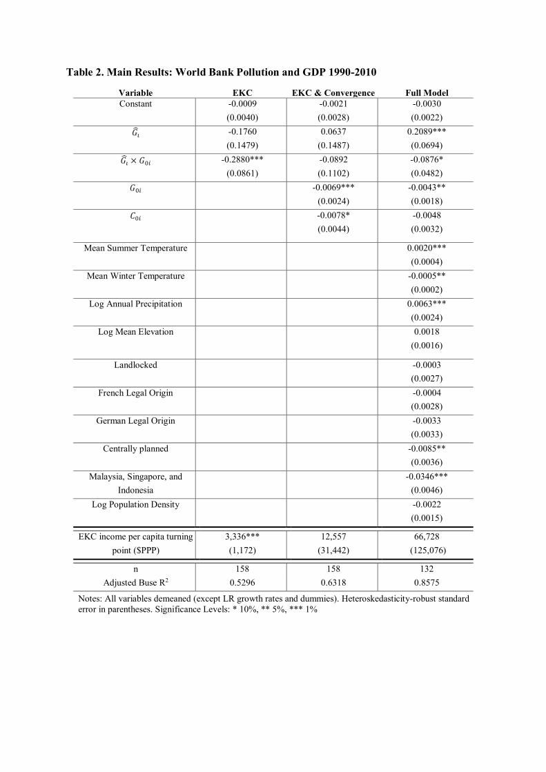
Table 2. Main Results: World Bank Pollution and GDP 1990-2010

Variable EKC EKC & Convergence Full Model

Constant -0.0009

(0.0040)

-0.0021

(0.0028)

-0.0030

(0.0022)

𝐺�̂� -0.1760

(0.1479)

0.0637

(0.1487)

0.2089***

(0.0694)

𝐺�̂� × 𝐺0𝑖 -0.2880***

(0.0861)

-0.0892

(0.1102)

-0.0876*

(0.0482)

𝐺0𝑖 -0.0069***

(0.0024)

-0.0043**

(0.0018)

𝐶0𝑖 -0.0078*

(0.0044)

-0.0048

(0.0032)

Mean Summer Temperature 0.0020***

(0.0004)

Mean Winter Temperature -0.0005**

(0.0002)

Log Annual Precipitation 0.0063***

(0.0024)

Log Mean Elevation 0.0018

(0.0016)

Landlocked -0.0003

(0.0027)

French Legal Origin -0.0004

(0.0028)

German Legal Origin -0.0033

(0.0033)

Centrally planned -0.0085**

(0.0036)

Malaysia, Singapore, and

Indonesia

-0.0346***

(0.0046)

Log Population Density -0.0022

(0.0015)

EKC income per capita turning

point ($PPP)

3,336***

(1,172)

12,557

(31,442)

66,728

(125,076)

n 158 158 132

Adjusted Buse R2 0.5296 0.6318 0.8575

Notes: All variables demeaned (except LR growth rates and dummies). Heteroskedasticity-robust standard

error in parentheses. Significance Levels: * 10%, ** 5%, *** 1%

Table 3. Robustness Checks

Variable OLS WB Data

1990-2010

WLS WB Data

1990-2000

WLS WB

Data

2000-2010

WLS PWT

Income

1990-2010

WLS EPI

Pollution

2000-2010

Constant 0.0004

(0.0021)

-0.0054***

(0.0018)

-0.0033

(0.0037)

-0.0025

(0.0026)

0.0073

(0.0047)

𝐺�̂� 0.0307

(0.0540)

0.1838***

(0.0510)

0.4309***

(0.1398)

0.2343***

(0.0702)

0.3729***

(0.1101)

𝐺�̂� × 𝐺0𝑖 -0.0247

(0.0412)

-0.0292

(0.0509)

0.1006

(0.0740)

0.1453**

(0.0651)

0.0265

(0.0971)

𝐺0𝑖 -0.0021*

(0.0011)

-0.0056***

(0.0019)

-0.0052*

(0.0028)

-0.0106***

(0.0021)

-0.0118***

(0.0030)

𝐶0𝑖 -0.0056***

(0.0018)

-0.0039

(0.0031)

-0.0028

(0.0050)

-0.0051

(0.0031)

-0.0140***

(0.0029)

Mean Summer

Temperature

0.0013***

(0.0004)

0.0021***

(0.0005)

0.0019***

(0.0007)

0.0023***

(0.0004)

0.0030***

(0.0007)

Mean Winter

Temperature

-0.0002

(0.0002)

-0.0004*

(0.0003)

-0.0003

(0.0004)

-0.0008***

(0.0003)

-0.0013***

(0.0003)

Log Annual

Precipitation

0.0016

(0.0018)

0.0048

(0.0031)

0.0083***

(0.0032)

0.0096***

(0.0031)

0.0034

(0.0030)

Log Mean Elevation 0.0040***

(0.0008)

0.0069***

(0.0021)

0.0006

(0.0022)

0.0049***

(0.0016)

0.0028

(0.0020)

Landlocked 0.0011

(0.0023)

-0.0037

(0.0028)

-0.0030

(0.0037)

-0.0081***

(0.0024)

-0.0117**

(0.0052)

French Legal Origin -0.0034*

(0.0019)

-0.0012

(0.0021)

-0.0020

(0.0043)

-0.0046*

(0.0026)

-0.0194***

(0.0046)

German Legal Origin -0.0097***

(0.0034)

-0.0054

(0.0053)

0.0013

(0.0055)

-0.0042

(0.0040)

-0.0049

(0.0053)

Centrally planned -0.0047

(0.0032)

-0.0087*

(0.0053)

-0.0072

(0.0057)

0.0028

(0.0040)

-0.0013

(0.0060)

Malaysia, Singapore,

and Indonesia

-0.0237***

(0.0029)

-0.0556***

(0.0030)

-0.0193**

(0.0095)

-0.0331***

(0.0043)

0.0044

(0.0053)

Log Population

Density

0.0004

(0.0007)

0.0021

(0.0025)

-0.0019

(0.0029)

0.0016

(0.0016)

0.0068***

(0.0017)

EKC income per

capita turning point

($PPP)

21,386

(74,564)

3,352,581

(40,156,293)

97

(249)

963

(549)

0.01

(0.26)

n 132 132 149 142 150

Adjusted Buse R2 0.5071 0.8777 0.8730 0.8258 0.8630

Notes: All variables demeaned (except LR growth rates and dummies). Heteroskedasticity-robust standard

error in parentheses. Significance Levels: * 10%, ** 5%, *** 1%

Figure 1. Growth Rates of PM 2.5 Pollution and GDP per Capita 1990-2010

Notes: Size of bubbles is proportional to population in 1990. Data source is World Bank

Development Indicators.

-7.5%

-5.0%

-2.5%

0.0%

2.5%

5.0%

-5% 0% 5% 10% 15% 20%

Growth Rate of GDP per Capita 1990-2010

Gro

wth

Rate

of

PM

2.5

19

90

-20

10