Quant Mark Econ (2010) 8:207–239DOI 10.1007/s11129-009-9073-0

Recording discrepancies in Nielsen Homescan data:Are they present and do they matter?

Liran Einav · Ephraim Leibtag · Aviv Nevo

Received: 18 September 2008 / Accepted: 17 July 2009 / Published online: 25 August 2009© Springer Science + Business Media, LLC 2009

Abstract We report results from a validation study of the Nielsen Homescanconsumer panel data. We use data from a large grocery retailer to matchtransactions that were recorded by the retailer (at the store) and by theHomescan panelist (at home). The matched data allow us to identify anddocument discrepancies between the two data sets in reported shopping trips,products, prices, and quantities. We find that the discrepancies are largestfor the price variable, and show that they are due to two effects: the first

We are grateful to two anonymous referees, to Peter Rossi (the Editor), and to participantsat the Chicago-Northwestern IO-Marketing conference, the Hoover Economics Bag Lunch,the NBER Price Dynamics Conference, the NBER Productivity Potpourri, the StanfordEconomics Junior Lunch, and the World Congress on National Accounts for many helpfulcomments. We thank Andrea Pozzi and Chris Taylor for outstanding research assistance.This research was funded by a cooperative agreement between the USDA/ERS andNorthwestern University, but the views expressed herein are those of the authors and do notnecessarily reflect the views of the U.S. Department of Agriculture.

L. EinavDepartment of Economics, Stanford University, Stanford, CA, USAe-mail: leinav@stanford.edu

L. Einav · A. NevoNBER, Cambridge, MA, USA

E. LeibtagUSDA/ERS, Washington, DC, USAe-mail: eleibtag@ers.usda.gov

A. Nevo (B)Department of Economics, Northwestern University, Evanston, IL, USAe-mail: nevo@northwestern.edu

208 L. Einav et al.

seems like standard recording errors (by Nielsen or the panelists), whilethe second is likely due to the way Nielsen imputes prices. We present twosimple applications to illustrate the impact of recording differences, and weuse one of the applications to illustrate how the validation study can beused to adjust estimates obtained from Nielsen Homescan data. The resultssuggest that while recording discrepancies are clearly present and potentiallyimpact results, corrections, like the one we employ, can be adopted by usersof Homescan to investigate the robustness of their results to such potentialrecording differences.

Keywords Measurement error · Validation study · Self-reported data

JEL Classification C81 · D12

1 Introduction

Nielsen Homescan (Homescan) is a large data set that tracks consumers’grocery purchases by asking consumers to scan barcodes of purchased productsat home after each shopping trip. The Homescan data allow researchers, prac-titioners, and policymakers to study questions that cannot be addressed usingother forms of data. For example, Homescan covers purchases at retailers thattraditionally do not cooperate with scanner data collection companies, such asWal-Mart and Whole Foods. Another advantage of the Homescan data is itsnational coverage, which provides wide variation in household location anddemographics compared to other panel data sets in which most householdsare from a small number of markets with relatively limited variation indemographics. Indeed, there has been a recent surge in the use of Homescanin the academic literature (Dube 2004; Aguiar and Hurst 2007; Hausman andLeibtag 2007; Katz 2007; and Broda and Weinstein 2008 and forthcoming).

Questions have been raised regarding the credibility of the Homescan datasince the data are self-recorded, and the recording process is time consuming.There are two common concerns. First, there are potential concerns aboutsample selection. Because of the time commitment, households who agreeto participate in the sample might not be representative of the populationof interest. Second, households who agree to participate in the sample mightrecord their purchases incorrectly.

This paper reports results from a validation study of the Homescan data thatallows us to examine the second concern—the accuracy of the recording. Weuse data from a single retailer to match records from Homescan with detailedtransaction-level data from the retailer. Thus, we are able to observe the sametransaction twice: as it was recorded by the retailer, and as recorded by theHomescan panelist. By comparing the two data sources we can documentreporting discrepancies (or lack thereof) and propose ways to correct for anyimplication these differences will have on statistical analysis. In particular, wecompare the data sets along two dimensions. First, we document differences

Recording discrepancies in Nielsen Homescan data 209

in trip and product information. If the household reported a trip that cannotbe found in the retailer data, we attribute this to mis-recorded trip information(store and/or date). Alternatively, if the household did not report a trip thatappears in the retailer data, we will consider this as an unreported trip.As we discuss later, this is the one and only statistic that relies on loyaltycard information and should be interpreted more cautiously as loyalty cardinformation is known to be noisy. Within matched trips, we document if thehousehold did not record or mis-recorded the product information. Second, formatched products, we document differences in the recording of the purchaseprice and quantity, and information on whether the product was purchased onpromotion.

Our goal is to present the results of our comparison and let future usersof Homescan decide whether they believe the discrepancies we report arepotentially a problem in their application. Our analysis proceeds in threesteps. First, we describe the magnitude of discrepancies between the twodata sets in different dimensions. Second, we investigate whether recordingdifferences are correlated with household or trip characteristics. Correlation ofrecording discrepancies with demographics may be suggestive of which typesof research would be most sensitive to such differences. For example, we askwhether a correlation between the price paid and demographics, observed inthe Homescan data, can be driven by systematic recording difference of priceby demographic groups. Third, we show how to correct for the reporting errors,and we provide sufficient information form our validation study to allow futureusers of Homescan who wish to perform the proposed correction to do so.

We would like to clarify two important issues more related to terminologythan to substance. First, through most of the paper we treat the retailer’s dataas the “truth,” allowing us to attribute any differences between the data setsto “errors” or “mistakes” in the Homescan data. Of course, to the extent thatthere are recording errors in the retailer’s data, these words should be inter-preted accordingly. We discuss this further in the context of the results. Second,we often refer to “errors,” “mistakes,” or “mis-recording” in Homescan. Thesecould be driven by various mechanisms that are discussed later in the paper:recording errors by the Homescan panelists themselves, misunderstanding ofthe Homescan instructions, or differences that are generated due to the wayNielsen puts together the data. We simply want to note that by using thewords “errors,” “mistakes,” or “mis-recording” we mean any of these possiblemechanisms.

In Section 2, we describe the study design and the data construction process.In Section 3, we document recording differences. For approximately 20% oftrips recorded in the Homescan data we can say with a high degree of certaintythat there is no corresponding transaction in the retailer’s data. This suggeststhat either the store or date information was recorded with error. Using theretailer’s loyalty card information, we find that there also seem to be manytrips that are found in the retailer’s data with no parallel in the Homescandata. Therefore, there seems to be evidence that households do not record allof their trips. For the trips we matched, we find that more than 10% of the

210 L. Einav et al.

items are not recorded. For those items recorded in both data sets, we findthat quantity is reported fairly accurately: 94% of the quantity informationmatches in the two data sets, and conditional on a reported quantity of 1 in theHomescan data, this probability goes up to 99%.

The match for the price variable is worse. In about half of the cases thetwo data sets do not agree. However, the correlation between the Homescanprice and the retailer’s price is 0.88, and the recording error explains onlyabout 22% of the variation in the reported price. We document two types ofprice errors. When the item is not associated with a loyalty card discount, theprice recording errors are similar to classical errors, and are roughly normallydistributed around the true price. In this case the correlation between the twoprices is 0.96 and the error explains only 8.5% of the variation in the Homescanprice. In contrast, when the item is associated with a loyalty card discount,prices in Homescan tend to over report the true price, sometimes by a largeamount. It seems likely that much of this second case is driven by the wayNielsen imputes prices. When available, Nielsen uses the quantity weightedaverage store-level price instead of the actual price paid by the household.The store-level price will differ from the price the panelist paid for at leasttwo reasons: loyalty card discounts and mid-week price changes. Both thesereasons are likely to contribute to the price recording errors we document. Wenote that this type of error might not be present for data from other retailersthat, for example, do not offer loyalty card discounts and do not change priceswithin a week, as defined by Nielsen.

We also investigate the heterogeneity across households in the quality oftheir data recording. We find that some households are extremely accurate,while others are much less so. We show that these latter households are morelikely to be larger households in which the female head of household is fullyemployed. This points to opportunity cost of time as an important determinantof recording errors in Homescan. Since we find that recording errors are notmean zero and are correlated with different household attributes, using theHomescan data may result in biased estimates of coefficients of interest, andmay lead to inaccurate conclusions. This motivates us to investigate how theserecording errors may affect results, and to propose ways to correct for theimpact of the recording errors. We present the impact of recording errors inthe context of two examples that use both the retailer and Homescan data. Wefirst study how the price paid varies with demographics, and we then estimatedemand. We also use the first example to illustrate how the validation samplecan be used to correct for recording errors. Indeed, we show that results usingthe true data and the Homescan data could be vastly different, and that ourcorrection procedure makes them closer.

For our correction method to be applicable more broadly in the Homescandata, we rely on the assumption that the distribution of the recording errors isthe same in our validation study as in the rest of the Homescan data. Becausethere is a reason to believe that our validation sample is not fully representativeof the entire Homescan data, corrections using our validation sample shouldbe done with caution and are probably best viewed as robustness checks.

Recording discrepancies in Nielsen Homescan data 211

This paper fits into a broader literature of validation studies. Responsesto surveys and self-reported data are at the heart of many data sets usedby researchers, executives, and policymakers. For example, the Panel Studyof Income Dynamics (PSID), the Current Population Survey (CPS), and theConsumer Expenditure Survey (CEX) are used heavily by economists. Oneconcern with self-reported data is that the data are recorded with error, andthat the error is systematically related to the characteristics of the respondentsor to the variables being recorded. Econometricians have developed theo-retical models to examine the consequences of measurement error. To studythe magnitude of the measurement error and to document the distribution ofthe error, an empirical literature has emerged that compares the self-reportedsample to a validation sample. Bound et al. (2001) provide a detailed reviewof this literature. This paper adds to this literature by examining a differentdata set and using a different validation method. While most of the literaturehas focused on data sets that record labor market decisions and outcomes,we study the Nielsen Homescan data, which documents purchase decisions.We compare the recording errors we document to errors in commonly usedeconomic data sets and find that errors in Homescan are of the same order ofmagnitude as errors in earnings and employment status data.

2 Data

2.1 Data sources

2.1.1 Homescan

The Homescan data consist of a panel of households who record their grocerypurchases.1 The purchases are from a wide variety of store types, includingtraditional food stores, non-traditional outlets such as supercenters and ware-house clubs, and online merchants. Consumers, who are at least 18 yearsold and interested in participating, register online and are asked to supplydemographic information. Based on this information, Nielsen contacts a subsetof these consumers. Consumers selected to become panel members are notpaid for participating in the program. However, every week a panel memberwho scans at least one purchase receives a set amount of points. The pointscan be redeemed for merchandise. Panelists can earn additional points foranswering surveys and by participating in sweepstakes that are open only topanel members.

Each participating household is provided with a scanner and instructed toscan all purchased items upon returning home after a given shopping trip. For

1See also http://www.nielsen.com/clients/index.html for additional information about the Homes-can data.

212 L. Einav et al.

each shopping trip the panelist is asked to identify the store from which itemswere purchased. They then scan the barcodes of the products they purchased,and enter the quantity of each item, whether the item was purchased atthe regular or promotional (“deal”) price, and the coupon amount (if used)associated with this purchase.

Nielsen then matches the barcode, or Universal Product Code (henceforthUPC), with detailed product characteristics. The recording of price is particu-larly important to understand some of the findings below. If the household pur-chased products at a store covered in Nielsen’s store-level data (“Scantrack”),Nielsen does not require the household to enter the price paid for each item (asa way to make the scanning process less time-consuming for the household).Instead, the price is imputed from the store-level data. We believe (but couldnot verify) that this imputation is used for all products bought at the retailer’sstores from which we obtained data. If the same item could be transacted atdifferent prices within the same store during the same week, this imputationprocess can introduce errors into the price data. Different consumers will paydifferent prices for (at least) two reasons. First, in some weeks discounts areoffered to loyalty card members and therefore consumers who use the loyaltycard will pay a lower price than those who do not use a loyalty card. Second,the retailer typically changes the price at most once a week, but oftentimes theprice changes do not align with the week definitions used for price imputationsby Nielsen. Therefore, consumers may pay a different price depending onwhich part of the week, as defined by Nielsen, they visited the store. As we willsee, this imputation process will lead to differences in price that are frequentand sometimes large.

In the analysis below we use data from 2004. We consider only householdsthat are part of the “static” sample, which contains households who reportpurchases in at least 10 months of the year. These households are generallyconsidered more reliable than those who report for fewer months, and theseare the only data available, to date, to researchers outside of Nielsen. Overall,the data include purchases of almost 250 million different items by just under40,000 households. We will focus on two metropolitan markets where theretailer has a significant presence. In these markets there are 1,249 householdsin Homescan who report over 900,000 items purchased.

2.1.2 The retailer’s data

The second data set comes from a large national grocery chain, which we willrefer to as “the retailer.” This retailer operates hundreds of stores across thecountry and records all the transactions in all of its stores. For each transaction,the data record the exact time of the transaction, the cashier number, andthe loyalty card number if one was used. The data list the UPCs purchased,the quantity purchased of each product, the price paid, and the loyalty carddiscount (if there was one). The retailer links loyalty cards that belong tomembers of the same household, primarily by matching the street addresses

Recording discrepancies in Nielsen Homescan data 213

and telephone numbers individuals use when applying for a loyalty card. Theretailer then assigns each household a unique identification number. Clearly,this definition of a household is more prone to errors than is Homescan’sdefinition, in which a household is simply associated with the house at whichthe scanner resides. We return to this later.

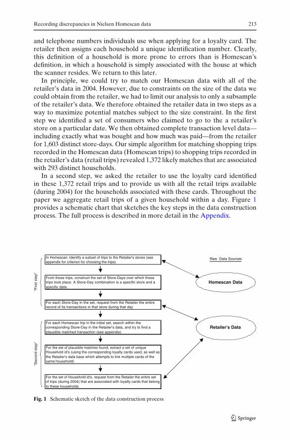
In principle, we could try to match our Homescan data with all of theretailer’s data in 2004. However, due to constraints on the size of the data wecould obtain from the retailer, we had to limit our analysis to only a subsampleof the retailer’s data. We therefore obtained the retailer data in two steps as away to maximize potential matches subject to the size constraint. In the firststep we identified a set of consumers who claimed to go to the a retailer’sstore on a particular date. We then obtained complete transaction level data—including exactly what was bought and how much was paid—from the retailerfor 1,603 distinct store-days. Our simple algorithm for matching shopping tripsrecorded in the Homescan data (Homescan trips) to shopping trips recorded inthe retailer’s data (retail trips) revealed 1,372 likely matches that are associatedwith 293 distinct households.

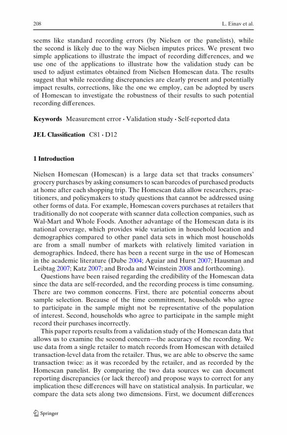
In a second step, we asked the retailer to use the loyalty card identifiedin these 1,372 retail trips and to provide us with all the retail trips available(during 2004) for the households associated with these cards. Throughout thepaper we aggregate retail trips of a given household within a day. Figure 1provides a schematic chart that sketches the key steps in the data constructionprocess. The full process is described in more detail in the Appendix.

In Homescan: Identify a subset of trips to the Retailer's stores (see appendix for criterion for choosing the trips)

Raw Data Sources

From these trips, construct the set of Store-Days over which these trips took place. A Store-Day combination is a specific store and a specific date.

Homescan Data

For each Store-Day in the set, request from the Retailer the entire record of its transactions in that store during that day

For each Homescan trip in the initial set, search within the corresponding Store-Day in the Retailer's data, and try to find a plausible matched transaction (see appendix)

Retailer's Data

For the set of plausible matches found, extract a set of unique Household id's (using the corresponding loyalty cards used, as well as the Retailer's data base which attempts to link multiple cards of the same household)

For the set of Household id's, request from the Retailer the entire set of trips (during 2004) that are associated with loyalty cards that belong to these households

"Sec

ond

step

""F

irst

ste

p"

Fig. 1 Schematic sketch of the data construction process

214 L. Einav et al.

Although the sample may seem a bit arbitrary, our sample selection methodis impartial. Our data selection criteria was meant to generate the mostmatches given our data extraction size limitations. Additionally, the retailerwas fully cooperative in the sense that the retailer provided all the data werequested. While we end up with a non-standard sample, we cannot think ofany reason that our sample selection would be correlated with any (potential)recording errors. We also want to emphasize that we only used the loyalty cardinformation to generate a data request. However, we did not use it for therecord-matching strategy. Therefore, unless we explicitly note, the statisticswe provide below will not be impacted by the way the retailer generates theloyalty card panel.

2.2 Record-matching strategy

We now describe our strategy for matching Homescan trips with retail trips.2

We start by analyzing possible matches in the data obtained in the first step.Recall that a Homescan trip contains all products purchased by the householdon a particular day in a particular store. The retailer’s data contain the productspurchased in each of the (more than 2,500 on average) retail trips at the samestore and day. The goal is to match the Homescan trip to exactly one of theretail trips in the retailer’s data, or to determine that none of the trips inthe retailer’s data is a good match. The latter case would be indicative of thehousehold misrecording the date or the store information in Homescan.

Since this procedure relies on the coding of the items (UPCs), one maybe concerned that certain items, especially non-packaged items, may havedifferent codes at the retailer’s stores and in Homescan. An additional concernis that the Homescan data we use only include the food items scanned bythe household, while the retailer data also include non-food items. To dealwith these concerns, we generated the universe of UPCs used by Homescanpanelists in the entire 2004 Homescan panel and, separately, the universe ofUPCs that are used by the retailer. We then restricted attention throughoutthe rest of the analysis to only the intersection of these two lists of UPCs (byeliminating from the analysis all data related to UPCs not in the intersection).Therefore, if a UPC is found in a retail trip but not in the correspondingHomescan trip, we can be sure that the UPC should have been recorded inthe Homescan data but was not for some reason.

After reducing the data set as described above, we continue as follows.Our unit of observation is a Homescan trip. For each such Homescan trip,

2Earlier we mentioned a simple matching algorithm we used for the data construction. This wasonly used to speed up the data requesting process from the retailer, and we do not use its resultsfurther. In this section we describe a more systematic matching strategy that is used for theremainder of the paper.

Recording discrepancies in Nielsen Homescan data 215

for which we have the retailer’s data for that store and that day, we count thenumber of distinct UPCs that overlap between the Homescan trip and eachof the hundreds of retail trips on the same date and in the same store. Wethen keep the two retail trips with the largest number of UPC overlap, anddefine ratios between the UPC overlap in each retail trip and the number ofdistinct UPCs reported for the Homescan trip. The first, r1, is the ratio of thenumber of overlapping UPCs in the retail trip with the highest overlap to thetotal number of distinct UPCs reported in the Homescan trip. The higher thisratio, the higher the fraction of products matched, and the more likely thatthis trip is a correct match. The second ratio, r2, is similar, but is computed forthe retail trip with the second-highest overlap. By construction, r2 will be lessthan or equal to r1. A higher r2 makes it more likely that the second retailtrip is also a reasonable match. Since, in reality, there is, at most, a singleretail trip that should be matched, this statistic tries to guard against a falsepositive. Our confidence in the match between the Homescan trip and the firstretail trip increases the higher is r1 and the lower is r2. As will become clearbelow, in practice it turns out that false positives resulting from this algorithmdo not seem to be a concern once the Homescan trip includes a large numberof distinct UPCs.

Using these two statistics, r1 and r2, and the number of products purchasedin the Homescan trip, we separate each Homescan trip into one of threecategories: reliable matches, Homescan trips that with high probability do nothave a match, and uncertain matches (i.e., we cannot classify these Homescantrips into either of the other groups with a reasonable level of certainty). Thefirst group of transactions will be used to study recording errors of products,prices, and quantities. The second group will be used to document unrecordedtrips or errors in recording trip information. We applied different criteriato define the three groups and verified that all our findings are robust toreasonable modifications of these criteria.

Matching Homescan trips to retail trips from the second step of the dataconstruction process is a slightly different task. Recall that here we are notsupplied with a list of all retail trips for the day and store. Instead, we aregiven a single retail trip that the retailer believes represents the household’spurchases on that day. Thus, the matching problem here is not which retail tripmatches the Homescan trip, but rather whether a given retail trip is a goodmatch or not. We match trips by computing the ratio r1, the number of distinctUPCs that overlap divided by the number of items in the Homescan trip. Usingthe statistic r1 and the total number of distinct items purchased, we classifythe Homescan trips into three categories, as we do with the first step data.In principle, in this step the thresholds for r1 used to classify the trips can bedifferent from the thresholds used in the first step. It turns out, however, thatthe vast majority of r1s we compute are either close to one or close to zero,making the choice of a threshold largely irrelevant. As an additional guardagainst false positives, we also report some of the results when eliminatingfrom the data certain households that seem to be inconsistent in the way theyuse their loyalty cards.

216 L. Einav et al.

3 Documenting recording differences

We now summarize our main findings of recording errors in the Homescandata. We organize the discussion around the three dimensions of potentialerrors: trip information, product (UPC) information, and price/quantity infor-mation. As mentioned earlier, for most of what follows we treat the retailer’sdata as the “truth” and ask if, or how well, the Homescan trip matches it. Inthat sense, Homescan recording “errors” are defined as records that do notmatch the retailer’s data. Although it could be the case that the retailer’scashier is the one making the error, rather than the Homescan panelist, wethink that this is less likely, especially for analysis at the product, price, andquantity level. At the trip level, when we sometimes rely on loyalty cardinformation, it is not clear that the retailer’s data are necessarily more accurate.For example, if a household borrows a loyalty card once, then all the retail tripsassociated with that card will be linked to the household’s record. We discussthis further below.

3.1 Trip and product information

We separate Homescan trips according to the number of distinct UPCs in theHomescan data. A small trip is defined as one with 4 or fewer UPCs, a mediumtrip has 5–9 UPCs, and a large trip is a trip with 10 UPCs or more. A potentialconcern is that we have false positives, i.e., that we match trips incorrectly.Our preliminary analysis (summarized in Einav et al. 2008) found that forthe medium and large trips mis-classification of a match is not a concern. Thereal issue is whether a match exists at all, which can be diagnosed by focusingon r1.

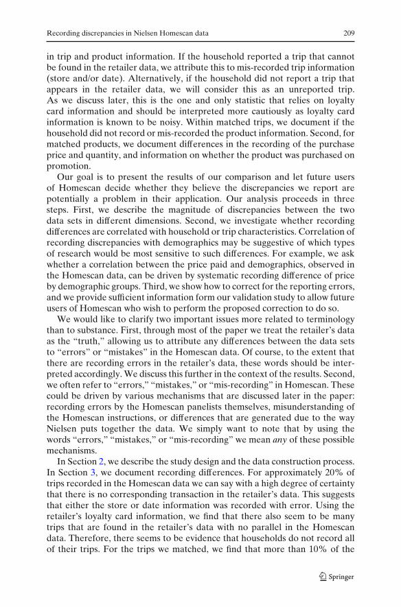
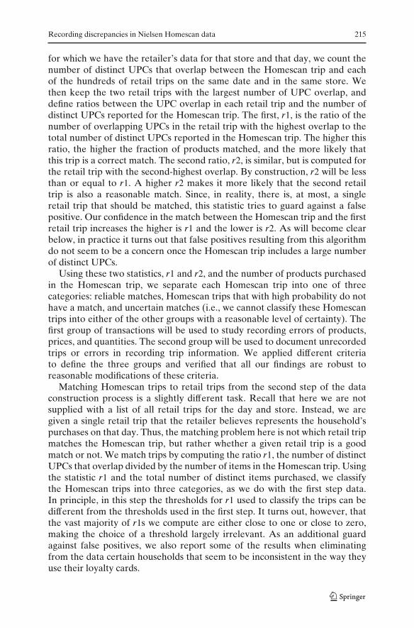
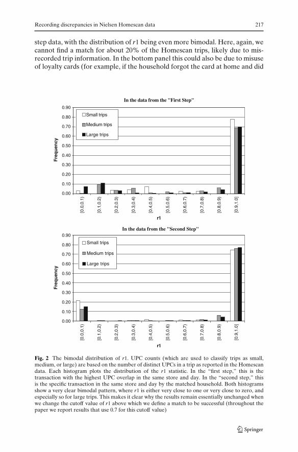
The distribution of r1 is displayed in Fig. 2. The information in the top panelhelps us address the question of how many of the Homescan trips that areassociated with the first step of the data construction process seem to havemis-recorded store and date information. Focusing on large trips, we find thatthere are 150 trips with r1 less than 0.2, 175 with r1 less than 0.3, and 180with r1 less than 0.4 (corresponding to 18.5, 21.6, and 22.4%, respectively).For medium trips the corresponding numbers are 113, 155, and 223 (or 9.5,13.0, and 18.7%). Taken together, these numbers suggest that for about 20%of the medium and large Homescan trips we can say with a high degree ofcertainty that they do not match any retail trip. Therefore, we conclude thatapproximately 20% of the Homescan trips have mis-recorded date or storeinformation.3 The bottom panel of Fig. 2 shows a similar pattern for the second

3A natural speculation is that some of these mis-recorded trips simply mis-record the date by aday (e.g., because the household did not get around to actually scanning the purchased products athome until the next day). Using the retailer’s data from the second step we found that while suchcases occur, they do not account for a large fraction of the 20% mis-recorded trips reported here.

Recording discrepancies in Nielsen Homescan data 217

step data, with the distribution of r1 being even more bimodal. Here, again, wecannot find a match for about 20% of the Homescan trips, likely due to mis-recorded trip information. In the bottom panel this could also be due to misuseof loyalty cards (for example, if the household forgot the card at home and did

In the data from the "First Step"

0.00

0.10

0.20

0.30

0.40

0.50

0.60

0.70

0.80

0.90

[0.0

,0.1

)

[0.1

,0.2

)

[0.2

,0.3

)

[0.3

,0.4

)

[0.4

,0.5

)

[0.5

,0.6

)

[0.6

,0.7

)

[0.7

,0.8

)

[0.8

,0.9

)

[0.9

,1.0

]

r1

Fre

qu

ency

0.00

0.10

0.20

0.30

0.40

0.50

0.60

0.70

0.80

0.90

Fre

qu

ency

Small trips

Medium trips

Large trips

In the data from the "Second Step"

[0.0

,0.1

)

[0.1

,0.2

)

[0.2

,0.3

)

[0.3

,0.4

)

[0.4

,0.5

)

[0.5

,0.6

)

[0.6

,0.7

)

[0.7

,0.8

)

[0.8

,0.9

)

[0.9

,1.0

]

r1

Small trips

Medium trips

Large trips

Fig. 2 The bimodal distribution of r1. UPC counts (which are used to classify trips as small,medium, or large) are based on the number of distinct UPCs in a trip as reported in the Homescandata. Each histogram plots the distribution of the r1 statistic. In the “first step,” this is thetransaction with the highest UPC overlap in the same store and day. In the “second step,” thisis the specific transaction in the same store and day by the matched household. Both histogramsshow a very clear bimodal pattern, where r1 is either very close to one or very close to zero, andespecially so for large trips. This makes it clear why the results remain essentially unchanged whenwe change the cutoff value of r1 above which we define a match to be successful (throughout thepaper we report results that use 0.7 for this cutoff value)

218 L. Einav et al.

not use it, the trip would be reported in Homescan but will not show up in thesecond step retailer’s data.) However, given that the fraction of unmatchedtrips in the top panel (where misuse of loyalty cards is not an issue) is verysimilar, we suspect that much of these unmatched trips are due to mis-recordedtrip information.

So far, we have looked for Homescan trips that cannot be matched to retailtrips. The data from the second step allow us to also look for the opposite case:retail trips that cannot be found in Homescan. Recall that the data obtained inthe second step include all the retail trips associated with certain households.We find that only 40% of these retail trips appear in Homescan, but we suspectthat this number is over estimating the fraction of missed trips, and that atleast part of it is driven by the retailer classifying multiple loyalty cards asbelonging to the same household, or by multiple households sharing the samecard. To address this concern, we focus on 273 households that seem to havemore reliable loyalty card use.4 On average, across these households, 53% ofthe retail trips are not reported in Homescan.

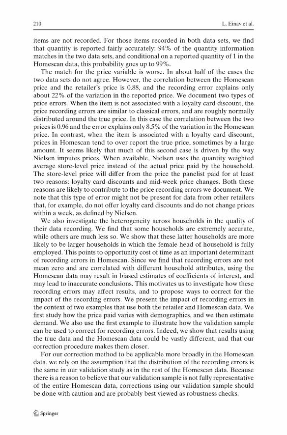
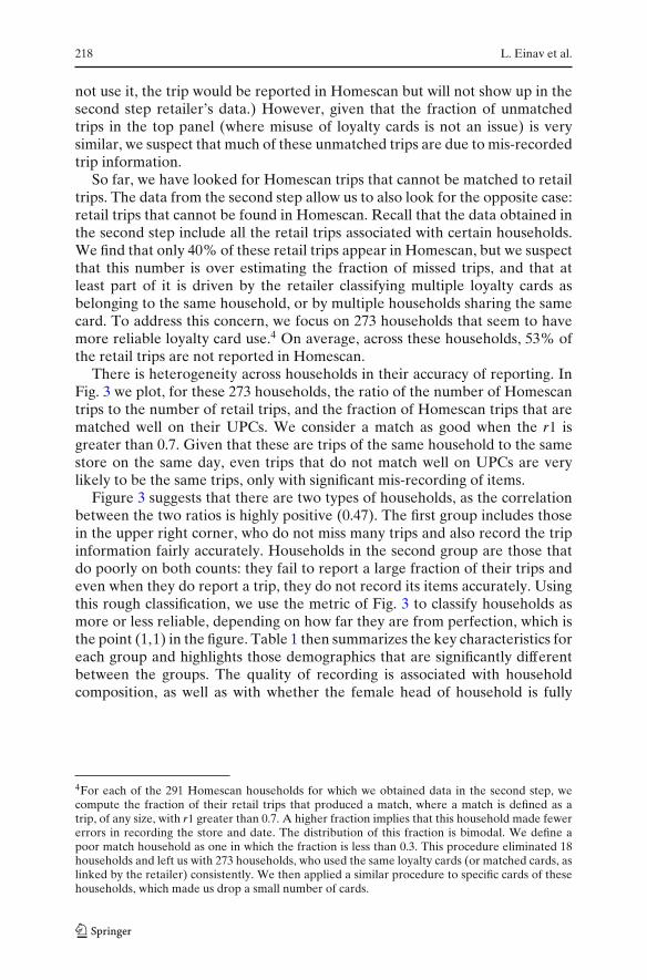
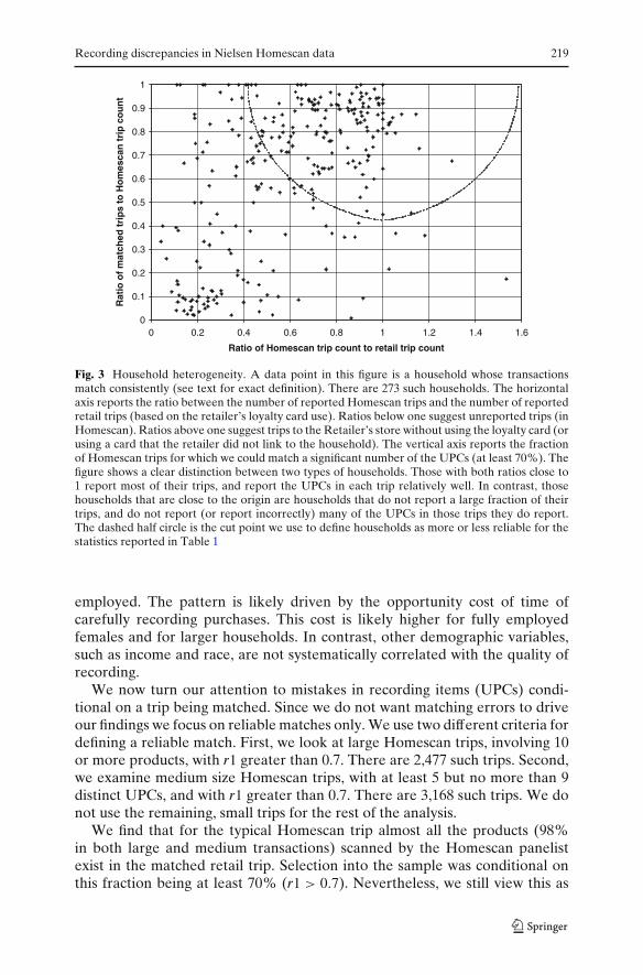
There is heterogeneity across households in their accuracy of reporting. InFig. 3 we plot, for these 273 households, the ratio of the number of Homescantrips to the number of retail trips, and the fraction of Homescan trips that arematched well on their UPCs. We consider a match as good when the r1 isgreater than 0.7. Given that these are trips of the same household to the samestore on the same day, even trips that do not match well on UPCs are verylikely to be the same trips, only with significant mis-recording of items.

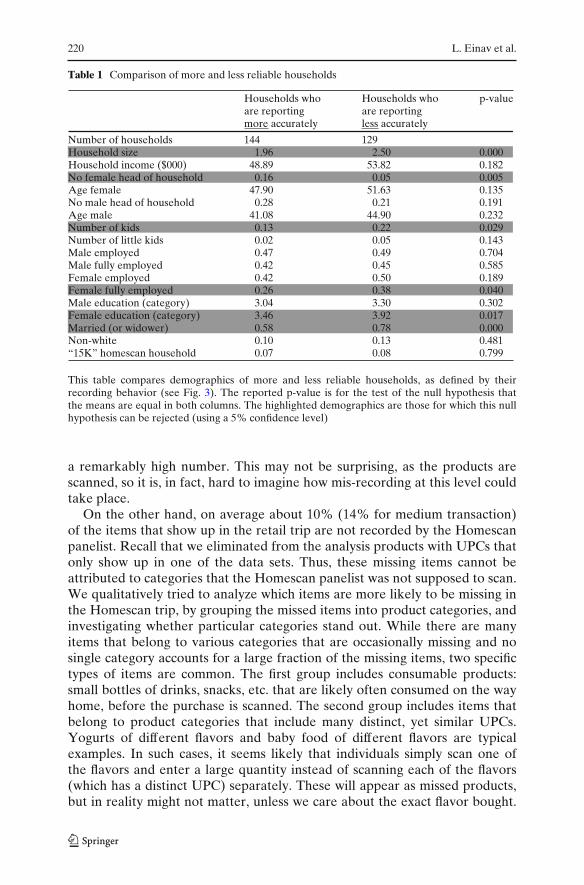
Figure 3 suggests that there are two types of households, as the correlationbetween the two ratios is highly positive (0.47). The first group includes thosein the upper right corner, who do not miss many trips and also record the tripinformation fairly accurately. Households in the second group are those thatdo poorly on both counts: they fail to report a large fraction of their trips andeven when they do report a trip, they do not record its items accurately. Usingthis rough classification, we use the metric of Fig. 3 to classify households asmore or less reliable, depending on how far they are from perfection, which isthe point (1,1) in the figure. Table 1 then summarizes the key characteristics foreach group and highlights those demographics that are significantly differentbetween the groups. The quality of recording is associated with householdcomposition, as well as with whether the female head of household is fully

4For each of the 291 Homescan households for which we obtained data in the second step, wecompute the fraction of their retail trips that produced a match, where a match is defined as atrip, of any size, with r1 greater than 0.7. A higher fraction implies that this household made fewererrors in recording the store and date. The distribution of this fraction is bimodal. We define apoor match household as one in which the fraction is less than 0.3. This procedure eliminated 18households and left us with 273 households, who used the same loyalty cards (or matched cards, aslinked by the retailer) consistently. We then applied a similar procedure to specific cards of thesehouseholds, which made us drop a small number of cards.

Recording discrepancies in Nielsen Homescan data 219

0

0.1

0.2

0.3

0.4

0.5

0.6

0.7

0.8

0.9

1

0 0.2 0.4 0.6 0.8 1 1.2 1.4 1.6

Ratio of Homescan trip count to retail trip count

Rat

io o

f m

atch

ed t

rip

s to

Ho

mes

can

tri

p c

ou

nt

Fig. 3 Household heterogeneity. A data point in this figure is a household whose transactionsmatch consistently (see text for exact definition). There are 273 such households. The horizontalaxis reports the ratio between the number of reported Homescan trips and the number of reportedretail trips (based on the retailer’s loyalty card use). Ratios below one suggest unreported trips (inHomescan). Ratios above one suggest trips to the Retailer’s store without using the loyalty card (orusing a card that the retailer did not link to the household). The vertical axis reports the fractionof Homescan trips for which we could match a significant number of the UPCs (at least 70%). Thefigure shows a clear distinction between two types of households. Those with both ratios close to1 report most of their trips, and report the UPCs in each trip relatively well. In contrast, thosehouseholds that are close to the origin are households that do not report a large fraction of theirtrips, and do not report (or report incorrectly) many of the UPCs in those trips they do report.The dashed half circle is the cut point we use to define households as more or less reliable for thestatistics reported in Table 1

employed. The pattern is likely driven by the opportunity cost of time ofcarefully recording purchases. This cost is likely higher for fully employedfemales and for larger households. In contrast, other demographic variables,such as income and race, are not systematically correlated with the quality ofrecording.

We now turn our attention to mistakes in recording items (UPCs) condi-tional on a trip being matched. Since we do not want matching errors to driveour findings we focus on reliable matches only. We use two different criteria fordefining a reliable match. First, we look at large Homescan trips, involving 10or more products, with r1 greater than 0.7. There are 2,477 such trips. Second,we examine medium size Homescan trips, with at least 5 but no more than 9distinct UPCs, and with r1 greater than 0.7. There are 3,168 such trips. We donot use the remaining, small trips for the rest of the analysis.

We find that for the typical Homescan trip almost all the products (98%in both large and medium transactions) scanned by the Homescan panelistexist in the matched retail trip. Selection into the sample was conditional onthis fraction being at least 70% (r1 > 0.7). Nevertheless, we still view this as

220 L. Einav et al.

Table 1 Comparison of more and less reliable households

Households who Households who p-valueare reporting are reportingmore accurately less accurately

Number of households 144 129Household size 1.96 2.50 0.000Household income ($000) 48.89 53.82 0.182No female head of household 0.16 0.05 0.005Age female 47.90 51.63 0.135No male head of household 0.28 0.21 0.191Age male 41.08 44.90 0.232Number of kids 0.13 0.22 0.029Number of little kids 0.02 0.05 0.143Male employed 0.47 0.49 0.704Male fully employed 0.42 0.45 0.585Female employed 0.42 0.50 0.189Female fully employed 0.26 0.38 0.040Male education (category) 3.04 3.30 0.302Female education (category) 3.46 3.92 0.017Married (or widower) 0.58 0.78 0.000Non-white 0.10 0.13 0.481“15K” homescan household 0.07 0.08 0.799

This table compares demographics of more and less reliable households, as defined by theirrecording behavior (see Fig. 3). The reported p-value is for the test of the null hypothesis thatthe means are equal in both columns. The highlighted demographics are those for which this nullhypothesis can be rejected (using a 5% confidence level)

a remarkably high number. This may not be surprising, as the products arescanned, so it is, in fact, hard to imagine how mis-recording at this level couldtake place.

On the other hand, on average about 10% (14% for medium transaction)of the items that show up in the retail trip are not recorded by the Homescanpanelist. Recall that we eliminated from the analysis products with UPCs thatonly show up in one of the data sets. Thus, these missing items cannot beattributed to categories that the Homescan panelist was not supposed to scan.We qualitatively tried to analyze which items are more likely to be missing inthe Homescan trip, by grouping the missed items into product categories, andinvestigating whether particular categories stand out. While there are manyitems that belong to various categories that are occasionally missing and nosingle category accounts for a large fraction of the missing items, two specifictypes of items are common. The first group includes consumable products:small bottles of drinks, snacks, etc. that are likely often consumed on the wayhome, before the purchase is scanned. The second group includes items thatbelong to product categories that include many distinct, yet similar UPCs.Yogurts of different flavors and baby food of different flavors are typicalexamples. In such cases, it seems likely that individuals simply scan one ofthe flavors and enter a large quantity instead of scanning each of the flavors(which has a distinct UPC) separately. These will appear as missed products,but in reality might not matter, unless we care about the exact flavor bought.

Recording discrepancies in Nielsen Homescan data 221

To measure this we examine the total number of items bought in the trip. Inthis example, the total quantity would match even if the distinct UPC countdoes not. This slightly reduces the differences, but not by much, implying thatmis-recorded quantity cannot fully explain the difference in the number ofproducts.

In order to check if the mistakes in recording products are systematic, weregress the missed expenditure on the total trip expenditure and find that alarger fraction of the expenditure is missed on larger trips. On large trips thehousehold is more likely to forget to scan, not go through the trouble of doingso, or consume items on the way home.

3.2 Price and quantity information

We now focus on errors in the recording of price and quantity variables. Forthis purpose we look at the products that appeared in both data sets from thereliably matched trips using the two definitions of reliable trips. It turns outthat the statistics we present below hardly vary across the groups, so matchreliability does not seem to be a concern. For the rest of this section we willrefer to the first set of matched products, those from Homescan trips with atleast 10 products and r1 greater than 0.7, as “matched large trips”; similarly, wewill refer to the products matched from medium Homescan trips as “matchedmedium trips.” For matched large trips we have 41,158 products purchased, anaverage of 16.6 products per trip. For matched medium trips we have 21,386matched items, for an average of 6.8 products per trip (recall that these aretrips with 5–9 products).

We present summary statistics for the key variables first and then discuss inmore detail additional patterns. Table 2 presents the fraction of observationsof quantity, expenditure, price, and deal indicator, that match between thereports in the Homescan data and in the retailer’s data. We present resultsseparately for large and medium trips to illustrate the robustness of thepatterns, but given that the summary statistics are so similar across these twotypes of trips, we focus the discussion and the subsequent analysis on largetrips alone. We find that 94% of the time the two data sources report the samequantity. The total expenditure on the item is the same in both data sets muchless frequently, and only 48% of the time do the two data sets report identicalexpenditure. On average, the expenditure reported in Homescan is about 10%higher than the expenditure recorded by the retailer, although there is widedispersion around this average (see Table 2). The pattern for price is similarto that of expenditure. It is slightly better matched (50% match rate and7% higher prices in Homescan on average), possibly because the expenditurevariable (price times quantity) is further prone to errors due to mis-recordedquantities. Finally, we examine the deal indicator. In the retailer’s data thedeal variable equals one if the gross and net price differ. In the Homescan datathis is a self reported variable. Overall, this indicator matches in 80% of theobservations, a worse match than the quantity data, but better than price.

222 L. Einav et al.

Table 2 Summary match statistics

Matched large trips Matched medium tripsMean Std. 5% 95% Mean Std. 5% 95%

QuantityHomescan 1.44 1.16 1 3 1.51 1.36 1 4Retailer 1.35 0.87 1 3 1.38 0.99 1 3Fraction same 0.938 0.924

ExpenditureHomescan 3.14 2.44 0.69 7.38 3.23 2.74 0.69 7.58Retailer 2.76 2.03 0.65 6.00 2.82 2.15 0.66 6.29Fraction same 0.479 0.486Log(homescan/retailer) 0.10 0.41 −0.38 0.69 0.10 0.44 −0.42 0.70

PriceHomescan 2.44 1.63 0.50 4.99 2.44 1.67 0.50 4.99Retailer 2.25 1.53 0.50 4.89 2.27 1.55 0.50 4.99Fraction same 0.503 0.512Log(homescan/retailer) 0.07 0.37 −0.37 0.61 0.05 0.39 −0.42 0.60

Deal indicatorHomescan 0.520 0.534Retailer 0.554 0.549Fraction same 0.795 0.820

Number of obs. (UPCs) 41,158 21,386Distinct shopping trips 2,477 3,168Distinct households 263 318

Large and medium trips are defined using the count of distinct UPCs as reported in Homescan(Medium: 5–9, Large: 10+). An observations in this table is a distinct item (UPC) in a given trip

We now explore in more detail the patterns we found for each of the vari-ables. We start with quantity. The overall match rate is reasonable. However,for 73% of the Homescan data and 76% of the retailer’s data (in matchedlarge trips), reported quantities are 1, so a high number of cases in which thetwo quantities are the same might not be surprising. Indeed, conditional onthe Homescan data reporting a quantity of 1, the probability of this reportmatching the retailer’s data is 0.99, while conditional of the Homescan datareporting a quantity larger than 1 the probability of a match is only 0.86. So areported quantity of 1 seems to be very reliable, while a quantity greater than1 might be somewhat more prone to mistakes, but still reasonable.

Using the data from the matched large trips, conditional on quantities notmatching, 82% of the time the quantity reported in Homescan is higher.Recording errors seem to be of various types, including six-packs that arerecorded as quantities of 6 (the fraction of mistakes for reported quantitiesof 6, 12, 18 and 24 are 0.60, 0.85, 1.00 and 0.78, respectively), typing errors(e.g., 11 instead of 1), and occasional “double scanning” (quantity of 2 insteadof 1). Together, this suggests that the Homescan data might be problematicfor studying the quantity purchased. It seems to be better suited to measurewhether or not a purchase occurred. Overall, the variance of error in thequantity variable constitutes 48.7% of the variance in the Homescan reportedquantity. The correlation coefficient between the two quantity variables is 0.72.

Recording discrepancies in Nielsen Homescan data 223

While in the case of quantity recording errors are likely driven by thepanelist’s recording error, the case of price is somewhat different, given ourunderstanding of how the Homescan prices are generated. As described inSection 2, if the consumer purchased the product at a store for which Nielsenhas store-level data, then the panelist is not asked to record the price paid.Instead, Nielsen imputes a price from the store-level data. If some of theshoppers in a store during a given week paid the full price while some got adiscount then the imputed price will be between the discounted price and non-discount price, and the Homescan data will over report or under report theactual transaction price. There are at least two reasons for heterogeneity inthe price paid in a particular week. First, some discounts are offered only toloyalty card holders. Analysis of the retailer data suggests that loyalty cardsare used in about 75–80% of the transactions,5 and that about 60% of thetransacted items are associated with loyalty card discounts, so errors due to thisdata construction process could be important. Second, even though typicallythe retailer changes the price at most once a week, the day when the pricechanges is in the middle of the week as defined by Nielsen. Thus, consumerswho purchase on different days might pay different prices.

This suggests that the recording errors in price may be either due to thepanelist’s recording error or due to the price imputation, and the statisticalproperties of these errors are likely different. Other retailers might not offerloyalty card discounts or set prices exactly in alignment with Nielsen’s defini-tion of a week; thus, the price imputation error might not be present in datafrom these retailers.

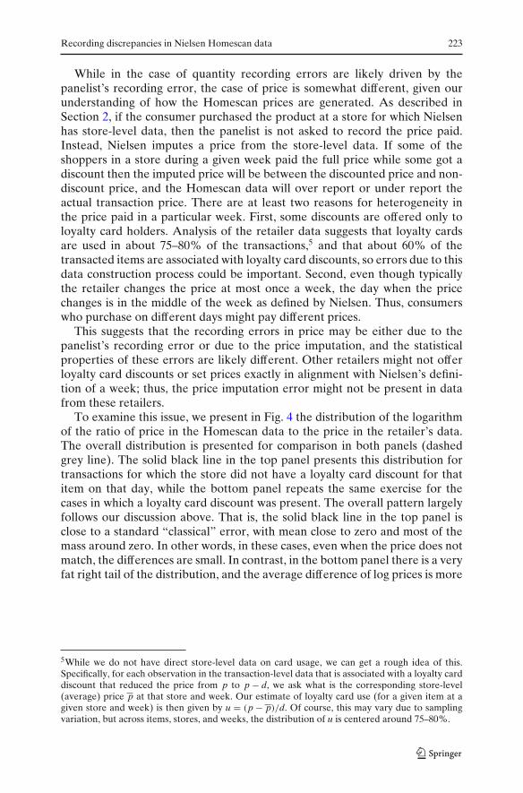
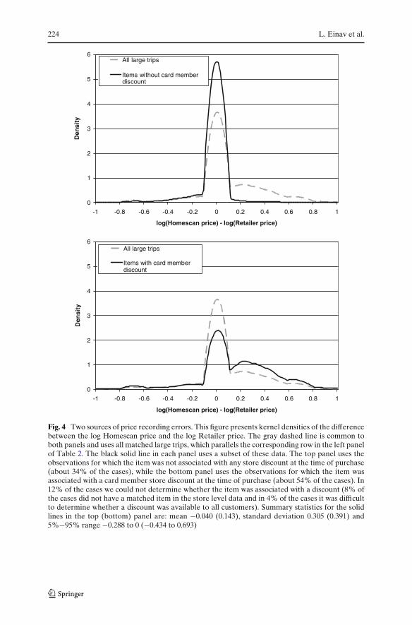
To examine this issue, we present in Fig. 4 the distribution of the logarithmof the ratio of price in the Homescan data to the price in the retailer’s data.The overall distribution is presented for comparison in both panels (dashedgrey line). The solid black line in the top panel presents this distribution fortransactions for which the store did not have a loyalty card discount for thatitem on that day, while the bottom panel repeats the same exercise for thecases in which a loyalty card discount was present. The overall pattern largelyfollows our discussion above. That is, the solid black line in the top panel isclose to a standard “classical” error, with mean close to zero and most of themass around zero. In other words, in these cases, even when the price does notmatch, the differences are small. In contrast, in the bottom panel there is a veryfat right tail of the distribution, and the average difference of log prices is more

5While we do not have direct store-level data on card usage, we can get a rough idea of this.Specifically, for each observation in the transaction-level data that is associated with a loyalty carddiscount that reduced the price from p to p − d, we ask what is the corresponding store-level(average) price p at that store and week. Our estimate of loyalty card use (for a given item at agiven store and week) is then given by u = (p − p)/d. Of course, this may vary due to samplingvariation, but across items, stores, and weeks, the distribution of u is centered around 75–80%.

224 L. Einav et al.

0

1

2

3

4

5

6

-1 -0.8 -0.6 -0.4 -0.2 0 0.2 0.4 0.6 0.8 1

log(Homescan price) - log(Retailer price)

Den

sity

All large trips

Items without card memberdiscount

0

1

2

3

4

5

6

-1 -0.8 -0.6 -0.4 -0.2 0 0.2 0.4 0.6 0.8 1

log(Homescan price) - log(Retailer price)

Den

sity

All large trips

Items with card memberdiscount

Fig. 4 Two sources of price recording errors. This figure presents kernel densities of the differencebetween the log Homescan price and the log Retailer price. The gray dashed line is common toboth panels and uses all matched large trips, which parallels the corresponding row in the left panelof Table 2. The black solid line in each panel uses a subset of these data. The top panel uses theobservations for which the item was not associated with any store discount at the time of purchase(about 34% of the cases), while the bottom panel uses the observations for which the item wasassociated with a card member store discount at the time of purchase (about 54% of the cases). In12% of the cases we could not determine whether the item was associated with a discount (8% ofthe cases did not have a matched item in the store level data and in 4% of the cases it was difficultto determine whether a discount was available to all customers). Summary statistics for the solidlines in the top (bottom) panel are: mean −0.040 (0.143), standard deviation 0.305 (0.391) and5%−95% range −0.288 to 0 (−0.434 to 0.693)

Recording discrepancies in Nielsen Homescan data 225

than 14%. This is consistent with the fact that all of our data is associated withusers of loyalty cards (this is how we matched them), while the price imputedfor them is aggregated over a population of which some do not use the loyaltycard. Therefore, imputed Homescan prices are higher in such cases.

Overall, the variance of the error in the price variable constitutes 21.8%of the variance in the Homescan price (8.5% if no loyalty card discountis offered). The correlation coefficient between the two price variables is0.88. The correlation increases to 0.96 if we condition on the Homescandeal indicator equal to 0 (and to 0.96 if we look at observations where noloyalty card discount was offered), and it decreases to 0.83 if the Homescandeal indicator is equal to 1 (0.84 if a loyalty card discount was offered). Thevariance in the error of the expenditure data explains 37.1% of the variationin the per item expenditure of the Homescan data. The correlation coefficientis 0.79.

In summary, we find that for the matched products, quantity is reportedfairly accurately, although, when quantity reported is higher than 1, thereported data are less accurate and therefore the correlation between the twoquantity variables is quite low. Prices and expenditures are reported with lessaccuracy. We suspect that this is due mostly to the Nielsen matching procedurethat imputes store-level prices when possible.

3.3 Comparison to measurement errors in other data sets

It may be useful to compare the magnitude and frequency of recording errorsin Homescan to those reported in other validation studies. To do so, we useBound et al. (2001, Section 6) who summarize the evidence on measurementerrors in data sets often used by labor economists. They report errors inearnings, transfer program income, assets, hours worked, unemployment sta-tus, industry and occupation, education, and health related variables. Whileit is hard to compare across contexts and over a large set of variables, ouroverall impression is that the magnitude of recording errors we document forHomescan are on the lower end of the range of recording errors reportedby Bound et al. (2001). For example, Bound and Krueger (1991) comparethe annual earnings reported in the CPS with Social Security administrativerecords. They find that the variance of the log of the ratio of earnings reportedin the two data sets is 0.114 for men and 0.051 for women. The correlationcoefficient between the two variables is 0.884 for men and 0.961 for women.Ashenfelter and Krueger (1994) study the years of schooling reported by twins:they compare the own report to the report of the twin. They find a correlationcoefficient of 0.9. We, on the other hand, find that the overall variance in thelog of the ratio of the Homescan and retailer price is 0.139. The variance isas low as 0.046 when the Homescan deal indicator is equal to zero, and 0.092if no loyalty card discount is offered. So overall it seems like the errors wedocument in Homescan are comparable to what is found in other commonlyused data sets.

226 L. Einav et al.

4 Correcting for recording errors

Up to this point we used the validation sample to document recording errors.In this section, we discuss how the validation sample can be used to control forrecording errors. Our discussion follows Chen et al. (2005), who provide moredetails and additional references. The basic idea is to use the validation sampleto learn the distribution of the error, conditional on variables observed in theprimary data. One can then use this distribution and “integrate over” it in theprimary data. Of course, a key assumption is that the (conditional) distributionof the error is the same in both the validation data and in the primary data. Thisassumption can be evaluated on a case-by-case basis, and we revisit it below inthe context of our application.

Formally, suppose the model we want to estimate implies a momentcondition:

E[m

(X∗, β0

)] =∫

m(x∗, β0) fX∗(x∗)dx∗ = 0 (1)

where m(·) is an r × 1 vector of known functions, X∗ are variables, which mightnot be fully observed, and β0 ∈ B, a compact subset of �q with 1 ≤ q ≤ r, is avector of the true value of unknown parameters that uniquely sets the momentcondition to zero. We observe two data sets. In the first, “primary” data set{Xpi : i = 1...Np}, we do not observe X∗, rather we only observe X, whichis measured with error of unknown form. In our context, Homescan is theprimary data set. In the second, “validation” data set we observe {(X∗

v j, Xv j) :j = 1...Nv}, i.e., both the variable that is measured with error and its truevalue. The matched Homescan-retailer data is the validation sample in ourcase. We denote by fX∗

p, fXp , fX∗

v, and fXv

, as the marginal densities of thelatent variable and the mis-measured variable in the primary and validationdata sets. We also denote by fX∗

p|Xp and fX∗v |Xv

the conditional densities of thelatent variable given the mis-measured variable in the primary and validationdata sets, respectively.

The key assumption is that

fX∗v |Xv=x = fX∗

p|Xp=x for all x. (2)

That is, that the distribution of the true variables, conditional on the observedvariables, is the same in both the primary and the validation samples. This isnot a trivial assumption. For example, to use our validation sample for theentire Homescan data, it would require that the recording error is the same forthe retailer we observe and for all other retailers. Even though we assume thatfX∗

v |Xv=x = fX∗p|Xp=x, we note the marginal density fXv

might be different thanfXp and therefore fX∗

vmight be different than fX∗

p.

We do not observe X∗ in the primary data set and therefore cannot directlyuse the moment condition in Eq. 1 to estimate β. However, we could use the

Recording discrepancies in Nielsen Homescan data 227

validation sample to estimate fX∗v |Xv

, and the primary data set to estimate fXp .Thus,

fX∗p(x∗) =

∫fX∗

p|Xp=x(x∗) fXp(x)dx =∫

fX∗v |Xv=x(x∗) fXp(x)dx (3)

where the second equality uses the key assumption that fX∗v |Xv=x = fX∗

p|Xp=x.

We can estimate this density by fX∗p(x∗) = ∫

fX∗v |Xv=x(x∗) fXp(x)dx where

fX∗v |Xv=x(x∗) is the estimate of the density of X∗

v conditional on Xv = x, andfXp(x) is the estimated density of Xp in the primary data. Now, we can use themoment condition to estimate the parameters of interest by

β = arg minβ

(∫m(x∗, β) fX∗

p(x∗)dx∗

)′W

(∫m(x∗, β) fX∗

p(x∗)dx∗

), (4)

where W is a positive definite symmetric weight matrix.While intuitive, this estimator involves estimating two distributions,

fX∗v |Xv=x(x∗) and fXp(x), potentially non-parametrically, and then using them

in a non-linear moment condition. Instead, Chen et al. (2005) propose todefine

g(x, β) ≡ E[m

(X∗

p, β)

|Xp = x]

=∫

m(x∗, β

)fX∗

p|Xp=x(x∗)dx∗. (5)

Note, that g(·) is a function of the variable measured with error Xp, that isobserved in the primary data set, rather than with respect to the true (latent)variable X∗

p. We can now apply the law of iterated expectations, so that

Ep[g(X, β0)

] = Ep

[E

[m

(X∗

p, β0

)|Xp = x

]]

= Ep

[E

[m

(X∗

p, β0

)]|Xp = x

]= E

[0|Xp = x

] = 0. (6)

Thus, the original moment condition implies that

Ep[g(X, β0)

] =∫

g (x, β0) fXp(x)dx = 0, (7)

and we can estimate the parameters of interest by

β = arg minβ

⎛

⎝ 1

Np

Np∑

i=1

g(Xpi, β)

⎞

⎠

′

W

⎛

⎝ 1

Np

Np∑

i=1

g(Xpi, β)

⎞

⎠ (8)

where W is a positive definite symmetric weight matrix, and g(Xpi, β) is anon-parametric estimate of g(Xpi, β), estimated using the validation sample.Using the validation sample to estimate g(Xpi, β) yields a consistent estimatebecause of the key assumption (Eq. 2). Chen et al. (2005) propose using aseries (sieve) estimator of g(x, β):

g(x, β) =Nv∑

j=1

m(

X∗v j, β

)pk (

Xv j)′ (

P′v Pv

)−1pk(x), (9)

228 L. Einav et al.

where {pl(x), l = 1, 2, ...} denotes a sequence of known basis functions,pknv (x) = (p1(x), ...pk(x))′ and Pv = (pk(Xv1)...pk(XvNv

))′ for an integer k thatincrease with the sample size Nv , such that k → ∞, and k/Nv → 0 as Nv → ∞.In words, g(x, β) is estimated by projecting it onto the basis functions. Ingeneral, the optimization in Eq. 8 is non-linear, but not more complex thanthe optimization implied by using the moment condition given in Eq. 1.

In a linear model this simplifies to a fairly simple procedure. For example,suppose we want to estimate a regression of price paid p∗ on demographics D,as we do in the next section. In the primary data (Homescan) we observe p andD, but we are concerned about possible recording errors in p. In the validationsample, the matched Homescan-retailer data, we observe p, p∗, and D, wherep is the Homescan-reported price and p∗ is the retailer-reported price. Wethen first use the validation data to regress the retailer’s price p∗ on p and D,to obtain, for example,

E(p∗|p, D) = D′β + α p. (10)

We then use the estimated coefficients, β and α, to construct E(p∗|p, D) in theHomescan data. Using Homescan, we then regress this predicted price on Dto obtain the error-adjusted estimates.

It may be instructive to present the simplest case, in which both theprediction and estimating equations are linear, and the set of covariates D isidentical. In this case, the “naive” regression in Homescan would be to regressp on D, while the corrected regression will be to regress D′β + α p on D. Ifthe true coefficient on D is γ , then the “naive” coefficient will be (roughly)γ−β

α. That is, with no measurement errors or with classical measurement error,

we would have α = 1 and β = 0, and no bias. However, either α = 1 (the casewhere the mean of measurement error is not zero) or β = 0 (which would ariseif the measurement error is correlated with D) will result in a bias.

5 Applications

In this section we illustrate the impact of measurement error and the proposedcorrection in the context of two applications. In the first application the price isthe dependent variable, while in the second example we explore an illustrativedemand equation in which price is a regressor.

5.1 An illustrative application I: price regressions

Recently, researchers have used Homescan to study how the prices paid varywith household demographics (e.g., Aguiar and Hurst 2007). We perform asimple version of such a study in order to evaluate the impact of recordingerrors. Our goal is twofold. First, the application provides a more meaningfulway to evaluate the importance of recording errors. That is, while describing

Recording discrepancies in Nielsen Homescan data 229

the recording errors is potentially interesting, it is not sufficient for determiningwhether the recording errors should be a serious concern. In this section we askif the recording errors matter for conclusions drawn from the analysis. Second,we use this application to demonstrate how one could use our validation studyto correct for recording errors in Homescan, and we hope that future users ofHomescan will do so too, at least as a robustness check.

We note that our goal here is not to replicate any particular study, justto demonstrate that the errors could have important implications for certainconclusions, and to show how the validation study can be used to addressthese errors. We chose this particular application for two reasons. First, it isimportant and active line of work, making it more likely that researchers whouse Homescan will perform a similar analysis. Second, it is simple. The keyregression here is linear, and has price on the left hand side. This makes thisanalysis robust to classical recording errors in the Homescan price, and it isonly non-classical recording errors that would lead to bias. Other settings, inwhich the model is non-linear or the variable of interest is on the right handside will make the analysis more sensitive to errors, and the correction slightlymore complex.

The regression of interest in this application is

pik = αk + β ′ Di + εik (11)

where i is a household, k is a specific product (distinct UPC), p is the unitprice paid for this product,6 and Di is a vector of demographic characteristics.The αk’s are a set of UPC fixed effects, and β is a vector of coefficients ofinterest. The economic question is whether certain demographic groups paymore or less for the same product, relative to the rest of the population. Aguiarand Hurst (2007), for example, focus on the price paid over the life cycle andemphasize their finding that the elderly pay lower prices for the same item,compared to other age groups. One could analyze the corresponding effect ofother demographic groups, such as gender and race.

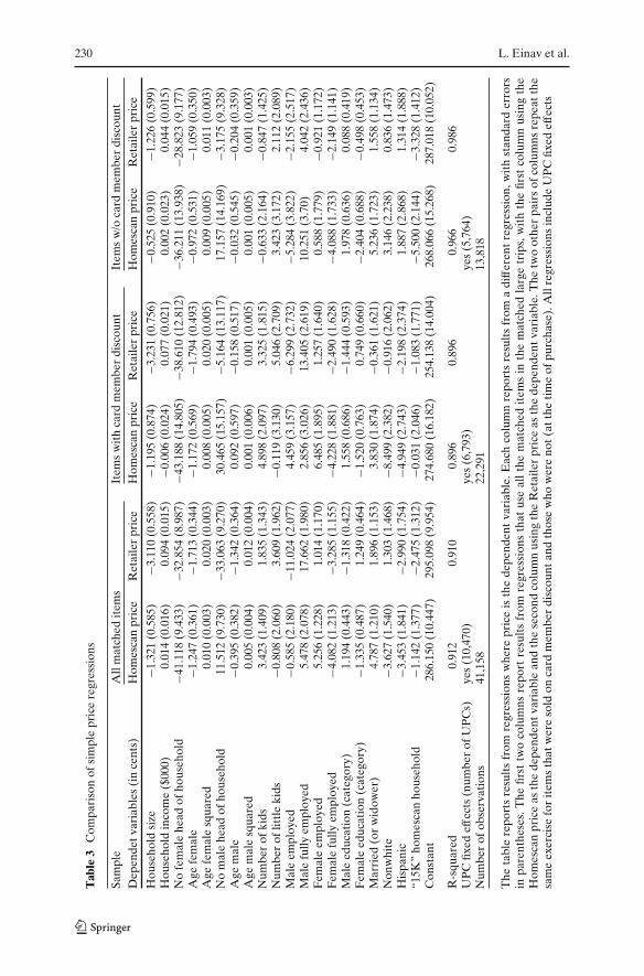
We start with Table 3, which presents results from estimating the aboveregression. An observation is a product (UPC) in a matched large trip, i.e.,in a large trip with r1 greater than 0.7. The regression reported in the firstcolumn uses as the dependent variable the price, in cents, as recorded inHomescan, while the regression reported in the second column uses the pricein the retailer’s data. The covariates are identical in both cases as is thesample, only the dependent variable is different. The results in the two columnsare somewhat different. Out of the twenty regression coefficients, five havedifferent signs, nine do not agree on their statistical significance, and thepoint estimate (when they have the same sign) are off by an average of morethan 40%.

6The reported results do not account for coupons. Results that use prices net of coupons arequalitatively similar, and are available from the authors upon request.

230 L. Einav et al.

Tab

le3

Com

pari

son

ofsi

mpl

epr

ice

regr

essi

ons

Sam

ple

All

mat

ched

item

sIt

ems

wit

hca

rdm

embe

rdi

scou

ntIt

ems

w/o

card

mem

ber

disc

ount

Dep

ende

tvar

iabl

es(i

nce

nts)

Hom

esca

npr

ice

Ret

aile

rpr

ice

Hom

esca

npr

ice

Ret

aile

rpr

ice

Hom

esca

npr

ice

Ret

aile

rpr

ice

Hou

seho

ldsi

ze−1

.321

(0.5

85)

−3.1

10(0

.558

)−1

.195

(0.8

74)

−3.2

31(0

.756

)−0

.525

(0.9

10)

−1.2

26(0

.599

)H

ouse

hold

inco

me

($00

0)0.

014

(0.0

16)

0.09

4(0

.015

)−0

.006

(0.0

24)

0.07

7(0

.021

)0.

002

(0.0

23)

0.04

4(0

.015

)N

ofe

mal

ehe

adof

hous

ehol

d−4

1.11

8(9

.433

)−3

2.85

4(8

.987

)−4

3.18

8(1

4.80

5)−3

8.61

0(1

2.81

2)−3

6.21

1(1

3.93

8)−2

8.82

3(9

.177

)A

gefe

mal

e−1

.247

(0.3

61)

−1.7

13(0

.344

)−1

.172

(0.5

69)

−1.7

94(0

.493

)−0

.972

(0.5

31)

−1.0

59(0

.350

)A

gefe

mal

esq

uare

d0.

010

(0.0

03)

0.02

0(0

.003

)0.

008

(0.0

05)

0.02

0(0

.005

)0.

009

(0.0

05)

0.01

1(0

.003

)N

om

ale

head

ofho

useh

old

11.5

12(9

.730

)−3

3.06

3(9

.270

)30

.465

(15.

157)

−5.1

64(1

3.11

7)17

.157

(14.

169)

−3.1

75(9

.328

)A

gem

ale

−0.3

95(0

.382

)−1

.342

(0.3

64)

0.09

2(0

.597

)−0

.158

(0.5

17)

−0.0

32(0

.545

)−0

.204

(0.3

59)

Age

mal

esq

uare

d0.

005

(0.0

04)

0.01

2(0

.004

)0.

001

(0.0

06)

0.00

1(0

.005

)0.

001

(0.0

05)

0.00

1(0

.003

)N

umbe

rof

kids

3.42

3(1

.409

)1.

835

(1.3

43)

4.89

8(2

.097

)3.

325

(1.8

15)

−0.6

33(2

.164

)−0

.847

(1.4

25)

Num

ber

oflit

tle

kids

−0.8

08(2

.060

)3.

609

(1.9

62)

−0.1

19(3

.130

)5.

046

(2.7

09)

3.42

3(3

.172

)2.

112

(2.0

89)

Mal

eem

ploy

ed−0

.585

(2.1

80)

−11.

024

(2.0

77)

4.45

9(3

.157

)−6

.299

(2.7

32)

−5.2

84(3

.822

)−2

.155

(2.5

17)

Mal

efu

llyem

ploy

ed5.

478

(2.0

78)

17.6

62(1

.980

)2.

856

(3.0

26)

13.4

05(2

.619

)10

.251

(3.7

0)4.

042

(2.4

36)

Fem

ale

empl

oyed

5.25

6(1

.228

)1.

014

(1.1

70)

6.48

5(1

.895

)1.

257

(1.6

40)

0.58

8(1

.779

)−0

.921

(1.1

72)

Fem

ale

fully

empl

oyed

−4.0

82(1

.213

)−3

.285

(1.1

55)

−4.2

28(1

.881

)−2

.490

(1.6

28)

−4.0

88(1

.733

)−2

.149

(1.1

41)

Mal

eed

ucat

ion

(cat

egor

y)1.

194

(0.4

43)

−1.3

18(0

.422

)1.

558

(0.6

86)

−1.4

44(0

.593

)1.

978

(0.6

36)

0.08

8(0

.419

)F

emal

eed

ucat

ion

(cat

egor

y)−1

.335

(0.4

87)

1.24

9(0

.464

)−1

.520

(0.7

63)

0.74

9(0

.660

)−2

.404

(0.6

88)

−0.4

98(0

.453

)M

arri

ed(o

rw

idow

er)

4.78

7(1

.210

)1.

896

(1.1

53)

3.83

0(1

.874

)−0

.361

(1.6

21)

5.23

6(1

.723

)1.

558

(1.1

34)

Non

whi

te−3

.627

(1.5

40)

1.30

3(1

.468

)−8

.499

(2.3

82)

−0.9

16(2

.062

)3.

146

(2.2

38)

0.83

6(1

.473

)H

ispa

nic

−3.4

53(1

.841

)−2

.990

(1.7

54)

−4.9

49(2

.743

)−2

.198

(2.3

74)

1.88

7(2

.868

)1.

314

(1.8

88)

“15K

”ho

mes

can

hous

ehol

d−1

.142

(1.3

77)

−2.4

75(1

.312

)−0

.031

(2.0

46)

−1.0

83(1

.771

)−5

.500

(2.1

44)

−3.3

28(1

.412

)C

onst

ant

286.

150

(10.

447)

295.

098

(9.9

54)

274.

680

(16.

182)

254.

138

(14.

004)

268.

066

(15.

268)

287.

018

(10.

052)

R-s

quar

ed0.

912

0.91

00.

896

0.89

60.

966

0.98

6U

PC

fixed

effe

cts

(num

ber

ofU

PC

s)ye

s(1

0,47

0)ye

s(6

,793

)ye

s(5

,764

)N

umbe

rof

obse

rvat

ions

41,1

5822

,291

13,8

18

The

tabl

ere

port

sre

sult

sfr

omre

gres

sion

sw

here

pric

eis

the

depe

nden

tva

riab

le.E

ach

colu

mn

repo

rts

resu

lts

from

adi

ffer

ent

regr

essi

on,w

ith

stan

dard

erro

rsin

pare

nthe

ses.

The

first

two

colu

mns

repo

rtre

sult

sfr

omre

gres

sion

sth

atus

eal

lthe

mat

ched

item

sin

the

mat

ched

larg

etr

ips,

wit

hth

efir

stco

lum

nus

ing

the

Hom

esca

npr

ice

asth

ede

pend

entv

aria

ble

and

the

seco

ndco

lum

nus

ing

the

Ret

aile

rpr

ice

asth

ede

pend

entv

aria

ble.

The

two

othe

rpa

irs

ofco

lum

nsre

peat

the

sam

eex

erci

sefo

rit

ems

that

wer

eso

ldon

card

mem

ber

disc

ount

and

thos

ew

how

ere

not(

atth

eti

me

ofpu

rcha

se).

All

regr

essi

ons

incl

ude

UP

Cfix

edef

fect

s

Recording discrepancies in Nielsen Homescan data 231

It is interesting to note that in almost all the cases when a coefficient issignificant in one regression but not in the other, the retailer’s data generatethe significant estimate, while the Homescan data do not. In many cases thedifference is also economically meaningful. For example, in the Homescandata the coefficient on race dummy variable is negative and significant, whichimplies that non-white consumers pay a lower price. On the other hand, in theretailer’s data the coefficient is positive but not significant. A researcher usingthe Homescan data to study discrimination would probably reach differentconclusions than one using the retailer’s data to study the same question, usingthe very same set of shopping trips. Another example is in the impact of age onprice paid. The Homescan data suggest a flatter impact of age, especially formales, than the retailer’s data. Once again researchers using the data to studylife cycle consumption might reach incorrect conclusions using the Homescandata.

As already noted in the previous section, there are two effects that cause thedifference in the results. One is of pure recording errors, while the other arisesfrom the way Nielsen imputes prices. We separate items that were purchasedwith a loyalty card discount and those without a discount to identify cases inwhich one type of recording error is more likely than the other (just as wedid in generating Fig. 4). We then repeat the same regressions for these twodifferent cases, separately. In general, the regression results are quite differentfor each of the regression pairs, but the differences are much more subtle inthe case in which price imputation is likely to be an issue (when the itemwas associated with a loyalty card discount). For example, in the results forproducts with loyalty card discounts, the coefficient signs do not agree for eightout of the twenty coefficients. When a loyalty card discount is not available forthe item and price imputation is unlikely to introduce errors, only two of thepoint estimates do not agree in sign.

The channels by which the coefficients are biased are quite different de-pending on the nature of the recording errors. Consider the case in which therecording errors are driven by Nielsen’s price imputation, and focus on therace dummy variable. In this case, the regression using the Homescan data tellsus that non-white households tend to buy at cheaper stores, i.e., stores wherethe average consumer in the store pays less for the same item. The regressionusing the retailer’s data tells us that despite going to cheaper stores non-whitepanelists do not pay less on average. In contrast, the channel is different ifnone of the prices are imputed and the only difference is due to recordingmistakes made by the panelist. Once again we use the race dummy variablesas an example. The regression using the Homescan data tells us that non-whiteconsumers report a lower price. On the other hand, the regression using theretailer’s data suggests that they do not actually pay less, maybe even slightlymore. Together these suggest that white consumers tend to over report pricesrelative to non-white consumers, not that they are likely to pay more.

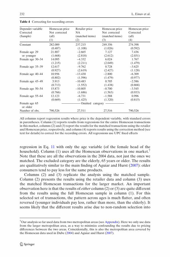
In order to further study the effect of recording errors and to illustratehow the validation study can be used to fix them, Table 4 presents Homescanregressions in which we only focus on the age effect. That is, we use the

232 L. Einav et al.

Table 4 Correcting for recording errors

Dependet variable Homescan price Retailer price Homescan price Homescan priceCorrected Not corrected NA Not corrected Corrected(Sample) (all) (matched items) (matched items) (all)

(1) (2) (3) (4)

Constant 282.089 237.215 249.356 274.398(0.487) (1.108) (1.026) (0.592)

Female age 29 21.887 –2.665 7.127 7.436or younger (1.668) (2.818) (2.612) (2.031)

Female age 30–34 14.095 –4.332 6.024 1.767(1.215) (2.211) (2.049) (1.479)

Female age 35–39 12.617 –9.762 0.728 –3.625(0.927) (2.619) (2.427) (1.128)

Female age 40–44 10.956 –13.430 –2.800 –6.309(0.802) (1.596) (1.479) (0.977)

Female age 45–49 5.913 –10.483 0.705 –2.586(0.713) (1.552) (1.438) (0.868)

Female age 50–54 15.873 –10.805 –0.700 –3.545(0.766) (1.686) (1.563) (0.933)

Female age 55–64 12.123 –6.731 –1.588 0.996(0.669) (1.425) (1.320) (0.815)

Female age 65 —————— Omitted category ——————or older

Number of obs. 790,526 27,511 27,516 790,526

All columns report regression results where price is the dependent variable, with standard errorsin parentheses. Column (1) reports results from regressions for the entire Homescan transactionsin this market, columns (2) and (3) report the results for the matched transactions using the retailerand Homescan price, respectively, and column (4) reports results using the correction method (seetext for details) to correct for the recording errors. All regressions use UPC fixed effects

regression in Eq. 11 with only the age variable (of the female head of thehousehold). Column (1) uses all the Homescan observations in one market.7

Note that these are all the observations in the 2004 data, not just the ones wematched. The excluded category are the elderly, 65 years or older. The resultsare qualitatively similar to the main finding of Aguiar and Hurst (2007): olderconsumers tend to pay less for the same products.

Columns (2) and (3) replicate the analysis using the matched sample.Column (2) presents the results using the retailer data and column (3) usesthe matched Homescan transactions for the larger market. An importantobservation here is that the results of either column (2) or (3) are quite differentfrom the results using the full Homescan sample in column (1). For thisselected set of transactions, the pattern across ages is much flatter, and oftenreversed (younger individuals pay less, rather than more, than the elderly). Itseems likely that the different results arise due to non-random selection into

7Our analysis so far used data from two metropolitan areas (see Appendix). Here we only use datafrom the larger metropolitan area, as a way to minimize confounding the results due to pricingdifferences between the two areas. Coincidentally, this is also the metropolitan area covered bythe Homescan data used in Dube (2004) and Aguiar and Hurst (2007).

Recording discrepancies in Nielsen Homescan data 233

our matched sample. For example, in the larger Homescan sample the elderlyare more likely to use coupons, while in our (matched) sample they are lesslikely to use them (not reported). It may not be totally surprising that thevalidation data is not representative of the larger Homescan data. We selecton matched trips, which are associated with more “careful” individuals. Thechange in the results between the matched and overall Homescan sample mayindicate that this selection is differential across age groups. For this reason weshould probably be careful in drawing conclusions based on either columns(2) or (3) of Table 4. On the other hand, the difference between the resultsin columns (2) and (3) also suggests that we should be careful in drawingconclusion based on column (1) because the results can potentially be drivenby recording errors.

In column (4) we present results that use the validation sample to correct forthe recording error. We follow the procedure described in the previous section.We first use the validation sample to predict the “true” retail price as a functionof the demographics (age dummies, in this case) and the Homescan reportedprice. We then use the full sample to impute predicted prices for each of theobservations and regress this predicted price on age. The resulting coefficientssignificantly change compared to column (1), and the age pattern is differentand economically less important. Loosely, the correction makes the estimatedcoefficients somewhere in between the original estimates (column (1)) and thetrue regression on the matched sample (column (2)).

We again note that an important assumption that makes this correction validis that the conditional distribution of recording errors is the same in the valida-tion sample and in the overall Homescan data (in that market). We note thatalthough it seems likely that the matched sample is non-randomly selected,this by itself does not violate the assumption; the conditional distribution ofthe recording errors may be the same even if the unconditional distribution ofprices is not. For this reason, we view this correction as a useful robustness testof existing estimates, rather than a recipe that should always be followed.

5.2 An illustrative application II: demand estimation

As a second application, we now illustrate the effect of measurement errorsin the context of demand estimation. Here price is a right hand side variable,so even classical measurement errors would lead to bias. Because we view thisexercise as illustrative, we favor making the comparison in the context of asimple and arguably more transparent model, rather than in a context of a full-blown demand system.8

8We note that our exercise is somewhat similar in spirit to the exercise reported by Gupta et al.(1996) who compare demand elasticities estimated from consumer-level data to those estimatedfrom store-level data. Unlike them, however, we use the same set of transactions, so we can focuson the measurement error; their results are likely driven by selection issues: consumers in the panelmight not represent the population of shoppers in the store.

234 L. Einav et al.

The basic regression we estimate in this exercise is

qik = αk + βk log pik + uik (12)

where i is a household, k is a specific product (distinct UPC), p is the unit pricepaid for this product, and q is the number of units bought. The αk’s are a setof UPC fixed effects, and βk’s are a set of product-specific semi-elasticities ofdemand.

We first estimate Eq. 12, using OLS, assuming the same semi-elasticitiesacross all products (that is, assuming βk = β for all k). The sample consists ofthe entire set of matched transactions (N = 41,158 as in the first column ofTable 3). Although the majority of transactions in our data have quantity (ofa given product in a given trip) equal to 1, in 25% of the transactions multipleunits of the same product are bought. Using the Homescan data, we obtain anestimate of the price semi-elasticity of −0.217 with a standard error of 0.018.In contrast, just as in the previous application, when we use the same set oftransactions, but use the price and quantity data as recorded by the retailer, weobtain a much greater (in absolute value) estimate of −0.503 with a standarderror of 0.020. The direction of the difference between the two estimates isconsistent with measurement errors in the Homescan price variable, whichwould bias the coefficient estimate toward zero. We note that repeating thesame exercise using the Homescan reported price and the retailer’s reportedquantity results in estimates that are almost the same as those that use bothprice and quantity from Homescan. This is consistent with our earlier reportthat the quantity variable is much less likely to significantly affect results, andthat the measurement errors in price are those driving the differences.

To investigate further, and to address a reasonable concern that the averageelasticity may be of less interest compared to the product-specific elasticity,we estimate Eq. 12 for each product separately. We focus on those productsthat are most frequently transacted. Specifically, we select the 28 products(UPCs) that are transacted at least 50 times in our matched sample. Twelve ofthese UPCs are different sizes and brands of milk, 6 of them are pre-packagedproduce (e.g., carrots and strawberries), and 10 are some other commonlypurchased items including carbonated soft drinks, sugar, and hotdog buns.Overall, this sample includes 2,570 matched transactions.9 We then reportthe results of the product-specific semi elasticities in Fig. 5. Each point inthe figure represents the semi-elasticity estimates for a given product; theestimates obtained from Homescan data are on the horizontal axis, and thoseobtained from the retailer data (using the same set of matched transactions)are on the vertical axis. The dashed line is the 45-degree line, so a pointbelow it represents a case in which the retailer data give rise to estimates ofgreater price sensitivity than the Homescan data. Overall, 23 out of the 28

9The average semi-elasticity in this selected sample is lower than that reported earlier, but thedifference between the data sets is similar. In this selected sample, we estimate semi-elasticities of−0.128 (0.022) and −0.378 (0.039) using the Homescan and the retailer data, respectively.

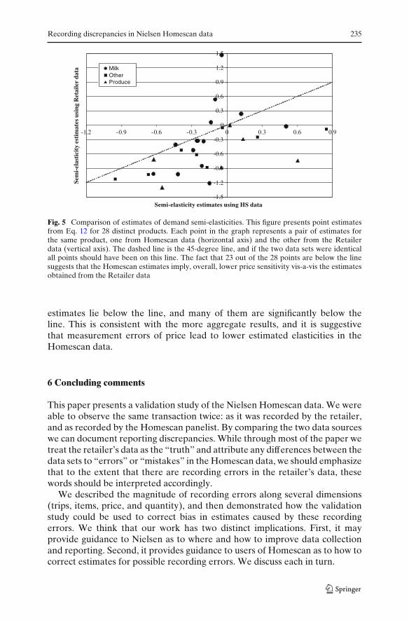
Recording discrepancies in Nielsen Homescan data 235

-1.5

-1.2

-0.9

-0.6

-0.3

0

0.3

0.6

0.9

1.2

1.5

-1.2 -0.9 -0.6 -0.3 0 0.3 0.6 0.9

Semi-elasticity estimates using HS data

Sem

i-el

asti

city

est

imat

es u

sing

Ret

aile

r da

ta MilkOtherProduce

Fig. 5 Comparison of estimates of demand semi-elasticities. This figure presents point estimatesfrom Eq. 12 for 28 distinct products. Each point in the graph represents a pair of estimates forthe same product, one from Homescan data (horizontal axis) and the other from the Retailerdata (vertical axis). The dashed line is the 45-degree line, and if the two data sets were identicalall points should have been on this line. The fact that 23 out of the 28 points are below the linesuggests that the Homescan estimates imply, overall, lower price sensitivity vis-a-vis the estimatesobtained from the Retailer data

estimates lie below the line, and many of them are significantly below theline. This is consistent with the more aggregate results, and it is suggestivethat measurement errors of price lead to lower estimated elasticities in theHomescan data.

6 Concluding comments

This paper presents a validation study of the Nielsen Homescan data. We wereable to observe the same transaction twice: as it was recorded by the retailer,and as recorded by the Homescan panelist. By comparing the two data sourceswe can document reporting discrepancies. While through most of the paper wetreat the retailer’s data as the “truth” and attribute any differences between thedata sets to “errors” or “mistakes” in the Homescan data, we should emphasizethat to the extent that there are recording errors in the retailer’s data, thesewords should be interpreted accordingly.

We described the magnitude of recording errors along several dimensions(trips, items, price, and quantity), and then demonstrated how the validationstudy could be used to correct bias in estimates caused by these recordingerrors. We think that our work has two distinct implications. First, it mayprovide guidance to Nielsen as to where and how to improve data collectionand reporting. Second, it provides guidance to users of Homescan as to how tocorrect estimates for possible recording errors. We discuss each in turn.

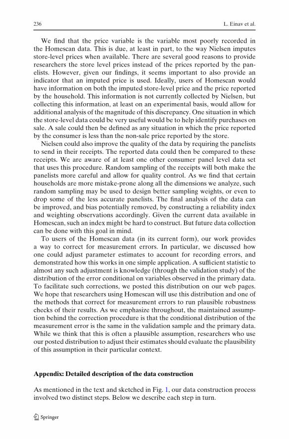
236 L. Einav et al.

We find that the price variable is the variable most poorly recorded inthe Homescan data. This is due, at least in part, to the way Nielsen imputesstore-level prices when available. There are several good reasons to provideresearchers the store level prices instead of the prices reported by the pan-elists. However, given our findings, it seems important to also provide anindicator that an imputed price is used. Ideally, users of Homescan wouldhave information on both the imputed store-level price and the price reportedby the household. This information is not currently collected by Nielsen, butcollecting this information, at least on an experimental basis, would allow foradditional analysis of the magnitude of this discrepancy. One situation in whichthe store-level data could be very useful would be to help identify purchases onsale. A sale could then be defined as any situation in which the price reportedby the consumer is less than the non-sale price reported by the store.

Nielsen could also improve the quality of the data by requiring the paneliststo send in their receipts. The reported data could then be compared to thesereceipts. We are aware of at least one other consumer panel level data setthat uses this procedure. Random sampling of the receipts will both make thepanelists more careful and allow for quality control. As we find that certainhouseholds are more mistake-prone along all the dimensions we analyze, suchrandom sampling may be used to design better sampling weights, or even todrop some of the less accurate panelists. The final analysis of the data canbe improved, and bias potentially removed, by constructing a reliability indexand weighting observations accordingly. Given the current data available inHomescan, such an index might be hard to construct. But future data collectioncan be done with this goal in mind.

To users of the Homescan data (in its current form), our work providesa way to correct for measurement errors. In particular, we discussed howone could adjust parameter estimates to account for recording errors, anddemonstrated how this works in one simple application. A sufficient statistic toalmost any such adjustment is knowledge (through the validation study) of thedistribution of the error conditional on variables observed in the primary data.To facilitate such corrections, we posted this distribution on our web pages.We hope that researchers using Homescan will use this distribution and one ofthe methods that correct for measurement errors to run plausible robustnesschecks of their results. As we emphasize throughout, the maintained assump-tion behind the correction procedure is that the conditional distribution of themeasurement error is the same in the validation sample and the primary data.While we think that this is often a plausible assumption, researchers who useour posted distribution to adjust their estimates should evaluate the plausibilityof this assumption in their particular context.

Appendix: Detailed description of the data construction

As mentioned in the text and sketched in Fig. 1, our data construction processinvolved two distinct steps. Below we describe each step in turn.

Recording discrepancies in Nielsen Homescan data 237

First step In principle, we could have asked the retailer to supply informationon any of its stores visited at any point by a Homescan panelist. However, sincegenerating the data involved some effort for the retailer we had to limit ourdata request, in the first step, to roughly fifteen hundred store-day transaction-level records.

We therefore proceeded as follows. First, we restricted the data set to twometropolitan areas, in which the retailer has high market share. This left uswith 265 different retailer stores (147 in one area, and 118 in the other). Sincewe identify the store by the zip code of its location, we restricted attentionto retailer stores that are the only retailer stores in the same zip code. Thiseliminated 76 stores (29%), and left us with 189 stores (101 in one area, 88 inthe other). We then searched the Homescan data for shopping trips at thesestores, with the additional conditions that: (i) the trip includes purchase of atleast 5 distinct UPCs (to make a match easier); (ii) the trip occurred afterFebruary 15, 2004 (to guarantee that the retailer, who deletes transaction-level data older than two years, still had these data at the time we put in thedata request); and (iii) the household shops at the retailer stores (accordingto Homescan) more than 20% and less than 80% of its trips. Our initial goalin generating the data was to study store choice; hence, we wanted consumerswho visited the retailer’s frequently, but not always. These trips were made by342 distinct households in the Homescan data. For 240 of these households,we randomly selected a single trip for each of them. For the remaining 102households, which included households with at least 10, and not more than 20,reported trips in Homescan data, we selected all their trips. We then requestedfrom the retailer the full transaction records for the store-days that matchedthese 1,779 trips. Since 74 of these trips were to the same store on the samedate, we expected to get 1,705 store-day transaction-level records.

We eventually got 1,603 of these 1,705 requested store-days (1,247 in thefirst area, 356 in the other), which account for 4,080,770 shopping trips. Themissing stores were mostly due to random coding errors when generating thedata. The retailer had little idea how we were going to match the data and hadno way to systematically impact our results by dropping data. They include122 distinct stores (74 in the first area, and 48 in the other). These 1,603store-days are associated with 1,675 trips from the sample of 1,779 shoppingtrips described above. However, since the retailer enjoys high market share inboth areas, it is not surprising that the 1,603 store-day transaction-level datarecords we obtained are associated with additional 904 trips in Homescan.These additional trips happened when two households in the Homescan panelvisited the same store on the same day, which is somewhat likely since themarket share of the retailer is high in the markets we studied. Given the waywe constructed the sample, however, many of these additional trips include asmall number of items, or households that rarely shop at the retailer’s stores.

Second step After obtaining the data from the first step, we developed asimple algorithm to find likely matches between trips in the Homescan datawith trips in the retailer’s data. These likely matches were only used to speed

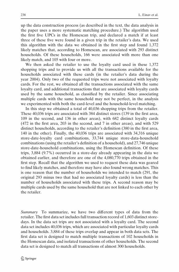
238 L. Einav et al.

up the data construction process (as described in the text, the data analysis inthe paper uses a more systematic matching procedure.) The algorithm usedthe first five UPCs in the Homescan trip, and declared a match if at leastthree of these five were found in a given trip in the retailer’s data. We usedthis algorithm with the data we obtained in the first step and found 1,372likely matches that, according to Homescan, are associated with 293 distincthouseholds. Of these households, 166 were associated with more than onelikely match, and 105 with four or more.

We then asked the retailer to use the loyalty card used in these 1,372shopping trips and to provide us with all the transactions available for thehouseholds associated with these cards (in the retailer’s data during theyear 2004). Only two of the requested trips were not associated with loyaltycards. For the rest, we obtained all the transactions associated with the sameloyalty card, and additional transactions that are associated with loyalty cardsused by the same household, as classified by the retailer. Since associatingmultiple cards with the same household may not be perfect, in the analysiswe experimented with both the card-level and the household-level matching.

In this step we obtained a total of 40,036 shopping trips from the retailer.These 40,036 trips are associated with 384 distinct stores (139 in the first area,109 in the second, and 136 in other areas), with 682 distinct loyalty cards(472 in the first area, 203 in the second, and 7 in other areas), and with 529distinct households, according to the retailer’s definition (380 in the first area,140 in the other). Finally, the 40,036 trips are associated with 34,316 uniquestore-date-loyalty card combinations, 33,744 unique store-data-householdcombinations (using the retailer’s definition of a household), and 27,746 uniquestore-date-household combinations, using the Homescan definition. Of thesetrips, 3,884 (9.7%) occurred in a store-day already appearing in the data weobtained earlier, and therefore are one of the 4,080,770 trips obtained in thefirst step. Recall that the algorithm we used to request these data was gearedto find likely matches, and therefore may have also found wrong matches. Thisis one reason that the number of households we intended to match (291, theoriginal 293 minus two that had no associated loyalty cards) is less than thenumber of households associated with these trips. A second reason may bemultiple cards used by the same household that are not linked to each other bythe retailer.

Summary To summarize, we have two different types of data from theretailer. The first data set includes full transaction record of 1,603 distinct store-days. In the data set trips are not associated with a loyalty card. The seconddata set includes 40,036 trips, which are associated with particular loyalty cardsand households. 3,884 of these trips overlap and appear in both data sets. Thefirst data set is designed to match multiple transactions of 102 households inthe Homescan data, and isolated transactions of other households. The seconddata set is designed to match all transactions of almost 300 households.

Recording discrepancies in Nielsen Homescan data 239

References

Aguiar, M., & Hurst, E. (2007). Life-cycle prices and production. American Economic Review,97(5), 1533–1559.

Ashenfelter, O., & Krueger, A. B. (1994). Estimates of the economic returns to schooling from anew sample of twins. American Economic Review, 84(5), 1157–1173.

Bound, J., Brown, C. C., & Mathiowetz, N. (2001). Measurement error in survey data. In E. E.Learner & J. J. Heckman (Eds.), Handbook of econometrics (pp. 3705–3843). New York:North Holland.

Bound, J., & Krueger, A. B. (1991). The extent of measurement error in longitudinal earningsdata: Do two wrongs make a right? Journal of Labor Economics, 9(1), 1–24.

Broda, C., & Weinstein, D. E. (2009). Product creation and destruction: Evidence and priceimplications. American Economic Review, in press.

Broda, C., & Weinstein, D. E. (2008). Understanding international price differences using barcodedata. NBER Working Paper No. 14017.

Chen, X., Hong, H., & Tamer, E. (2005). Measurement error models with auxiliary data. Reviewof Economic Studies, 72(2), 343–366.

Dube, J-P. (2004). Multiple discreteness and product differentiation: Demand for carbonated softdrinks. Marketing Science, 23(1), 66–81.

Einav, L., Leibtag, E., & Nevo, A. (2008). On the accuracy of Nielsen Homescan data. USDAEconomics Research Report Number 69.

Gupta, S., Chintagunta, P., Kaul, A., & Wittink, D. R. (1996). Do household scanner data pro-vide representative inferences from brand choices: A comparison with store data. Journal ofMarketing Research, 33(4), 383–398.

Hausman, J., & Leibtag, E. (2007). Consumer benefits from increased competition in shoppingoutlets: Measuring the effect of Wal-Mart. Journal of Applied Econometrics, 22(7), 1157–1177.

Katz, M. (2007). Estimating supermarket choice using moment inequalities. Ph.D. Dissertation,Harvard University.