randomized matrix algorithms and their applications to access my web page: petros drineas rensselaer...
Post on 19-Dec-2015
217 views
TRANSCRIPT

Randomized matrix algorithms and their applications
To access my web page:
Petros DrineasPetros Drineas
Rensselaer Polytechnic InstituteComputer Science Department
drineas
2
Randomized algorithms
Randomization and sampling allow us to design provably accurate algorithms for problems that are:
Massive
(e.g., matrices so large that can not be stored at all, or can only be stored in slow, secondary memory devices)
Computationally expensive or even NP-hard
(e.g., combinatorial problems such as the Column Subset Selection Problem)
3
Mathematical background
Obviously, linear algebra and probability theory. More specifically,
• Ideas underlying the design and analysis of randomized algorithms
E.g., the material covered in chapters 3, 4, and 5 of the “Randomized Algorithms” book of Motwani and Raghavan.
• Matrix perturbation theory
E.g., take a look at “Matrix Perturbation Theory” by Stewart and Sun, or “Matrix Analysis” by R. Bhatia.
4
Applying the math background
• Randomized algorithms
• By (carefully) sampling rows/columns/entries of a matrix, we can construct new matrices (that have smaller dimensions or are sparse) and have bounded distance (in terms of some matrix norm) from the original matrix (with some failure probability).
• By preprocessing the matrix using random projections (*), we can sample rows/columns/ entries(?) much less carefully (uniformly at random) and still get nice bounds (with some failure probability).
(*) Alternatively, we can assume that the matrix is “well-behaved” and thus uniform sampling will work.
5
Applying the math background
• Randomized algorithms
• By (carefully) sampling rows/columns/entries of a matrix, we can construct new matrices (that have smaller dimensions or are sparse) and have bounded distance (in terms of some matrix norm) from the original matrix (with some failure probability).
• By preprocessing the matrix using random projections, we can sample rows/columns/ entries(?) much less carefully (uniformly at random) and still get nice bounds (with some failure probability).
• Matrix perturbation theory
• The resulting smaller/sparser matrices behave similarly (in terms of singular values and singular vectors) to the original matrices thanks to the norm bounds.
In this talk, I will illustrate a few “Randomized Algorithms” ideas that have been leveraged in the analysis of randomized algorithms in linear algebra.
6
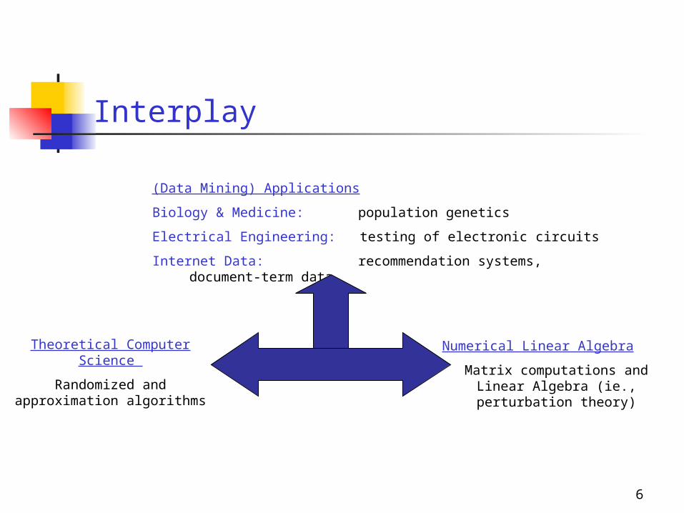
Interplay
Theoretical Computer Science
Randomized and approximation algorithms
Numerical Linear Algebra
Matrix computations and Linear Algebra (ie., perturbation
theory)
(Data Mining) Applications
Biology & Medicine: population genetics
Electrical Engineering: testing of electronic circuits
Internet Data: recommendation systems, document-term data
7
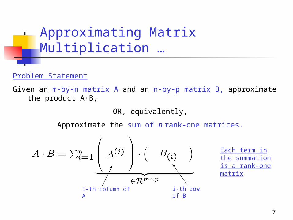
Approximating Matrix Multiplication …
Problem Statement
Given an m-by-n matrix A and an n-by-p matrix B, approximate the product A·B,
OR, equivalently,
Approximate the sum of n rank-one matrices.
Each term in the summation is a rank-one matrix
i-th column of A i-th row of B
8
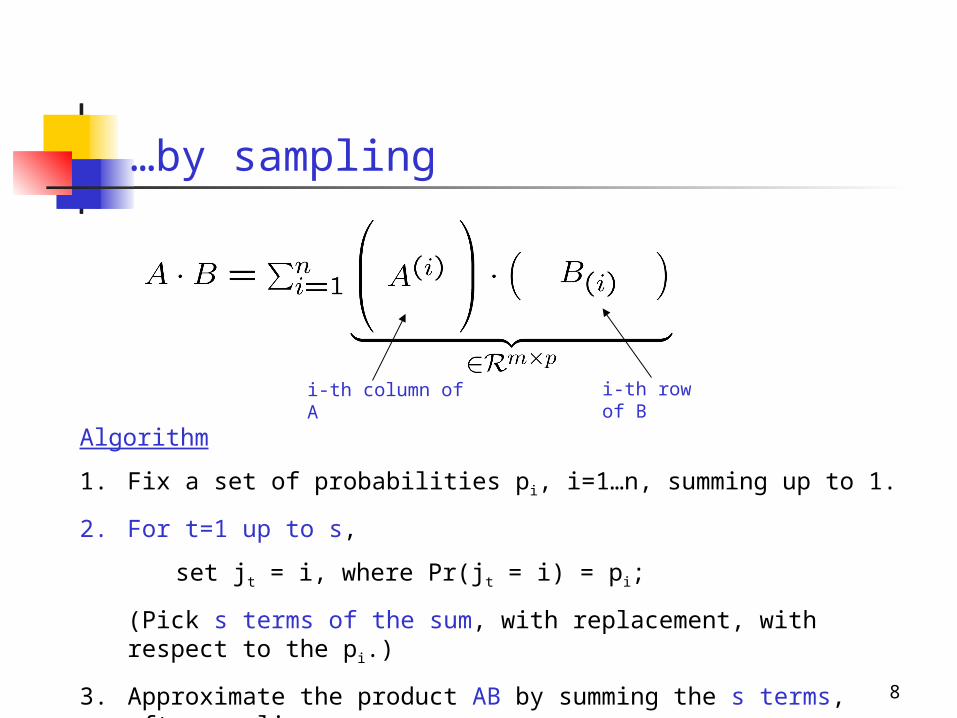
…by sampling
Algorithm
1. Fix a set of probabilities pi, i=1…n, summing up to 1.
2. For t=1 up to s,
set jt = i, where Pr(jt = i) = pi;
(Pick s terms of the sum, with replacement, with respect to the pi.)
3. Approximate the product AB by summing the s terms, after scaling.
i-th column of A i-th row of B
9
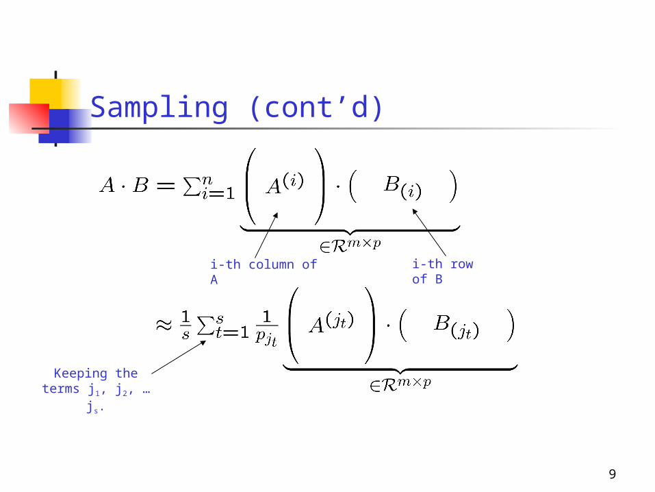
Sampling (cont’d)
i-th column of A i-th row of B
Keeping the terms j1, j2, … js.
10
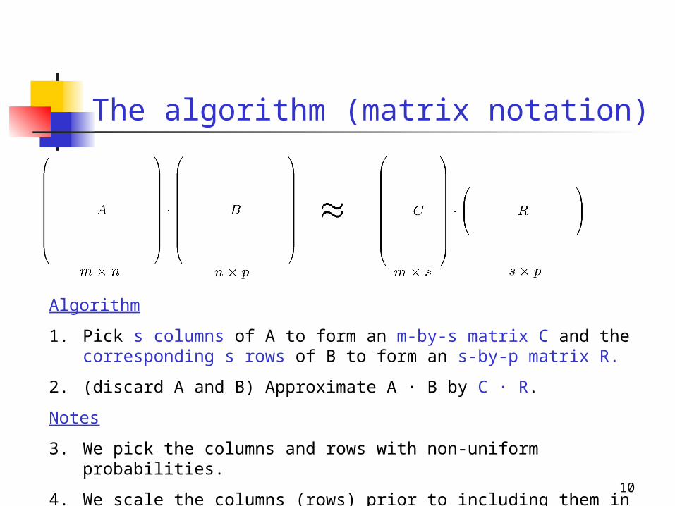
The algorithm (matrix notation)
Algorithm
1. Pick s columns of A to form an m-by-s matrix C and the corresponding s rows of B to form an s-by-p matrix R.
2. (discard A and B) Approximate A · B by C · R.
Notes
3. We pick the columns and rows with non-uniform probabilities.
4. We scale the columns (rows) prior to including them in C (R).
11
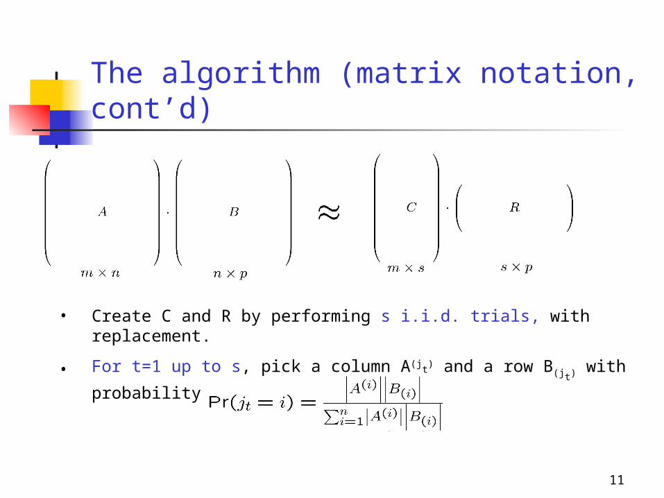
The algorithm (matrix notation, cont’d)
• Create C and R by performing s i.i.d. trials, with replacement.
• For t=1 up to s, pick a column A(jt) and a row B(jt)
with probability
• Include A(jt)/(spjt
)1/2 as a column of C, and B(jt)/(spjt
)1/2 as a row of
R.
12
Simple Lemmas …
• The expectation of CR (element-wise) is AB.
• Our adaptive sampling minimizes the variance of the estimator.
• It is easy to implement the sampling in two passes.
13
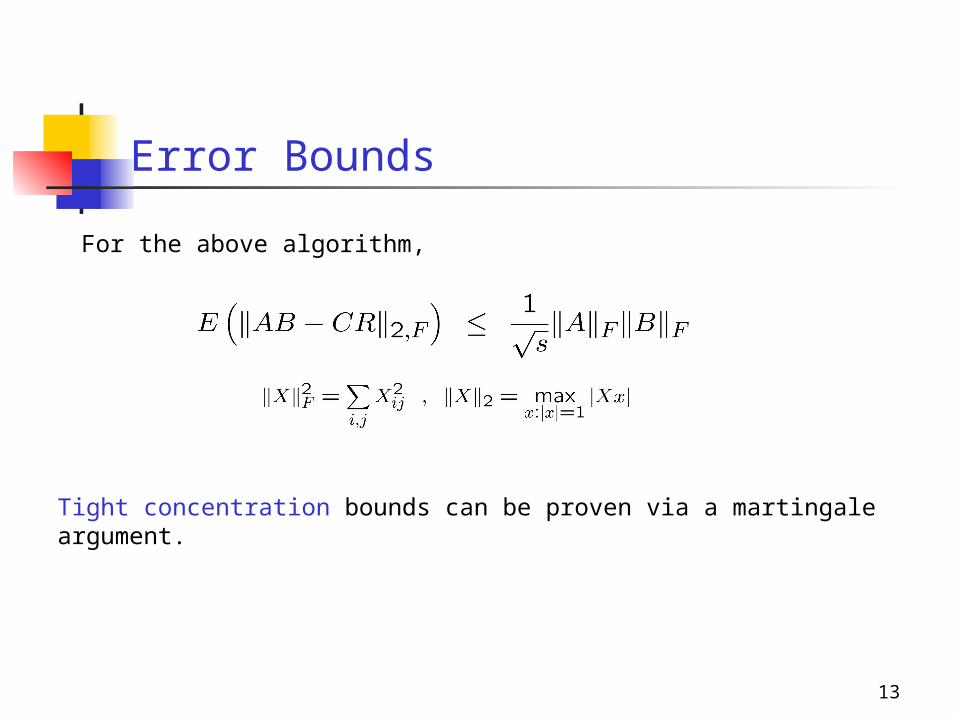
Error Bounds
For the above algorithm,
Tight concentration bounds can be proven via a martingale argument.
14
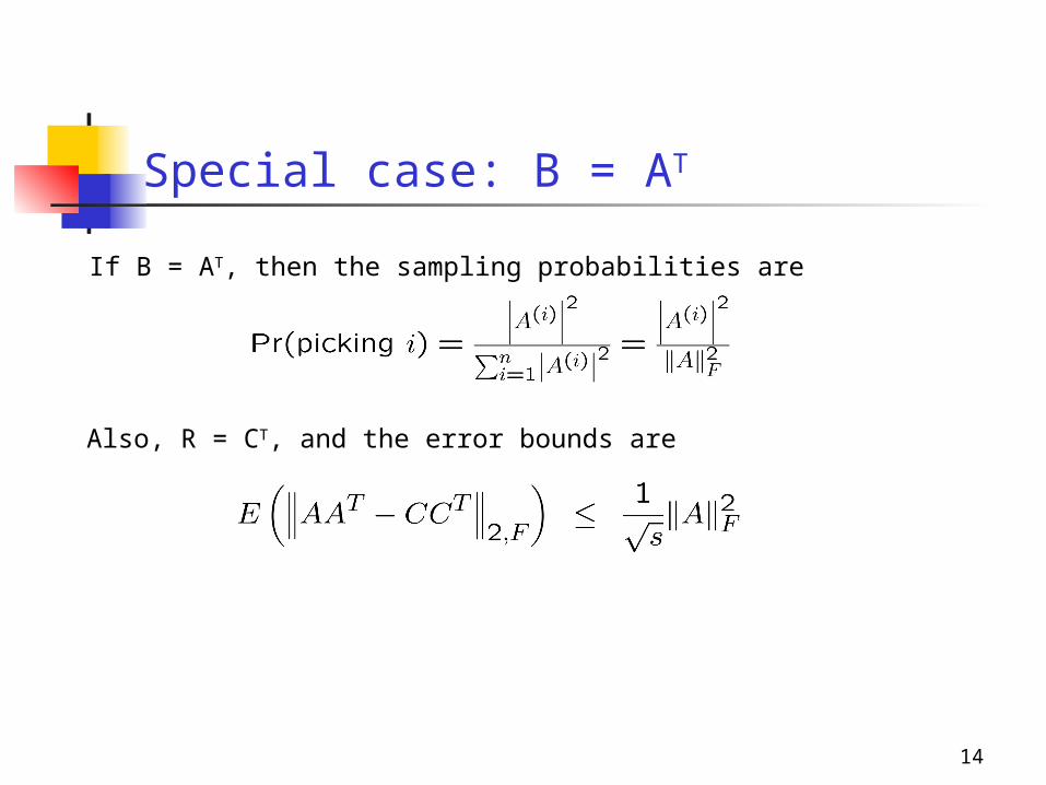
Special case: B = AT
If B = AT, then the sampling probabilities are
Also, R = CT, and the error bounds are
15
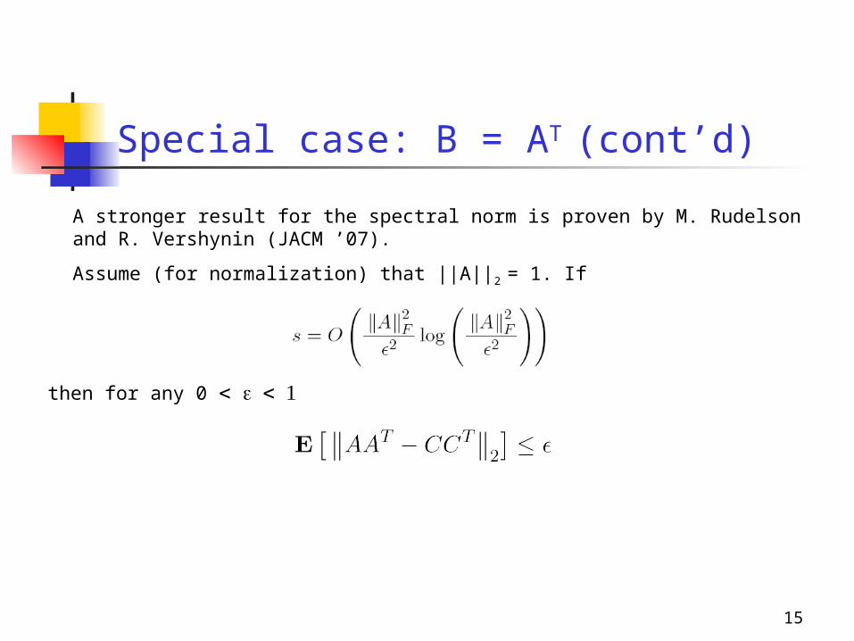
Special case: B = AT (cont’d)
A stronger result for the spectral norm is proven by M. Rudelson and R. Vershynin (JACM ’07).
Assume (for normalization) that ||A||2 = 1. If
then for any 0

16
Special case: B = AT (cont’d)
• Uses a beautiful result of M. Rudelson for random vectors in isotropic position.
• Tight concentration results can be proven using Talagrand’s theory.
• Notice that c has to be sufficiently large for the bound to hold.
A stronger result for the spectral norm is proven by M. Rudelson and R. Vershynin (JACM ’07).
Assume (for normalization) that ||A||2 = 1. If
then for any 0
17
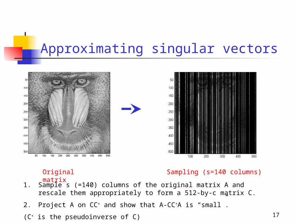
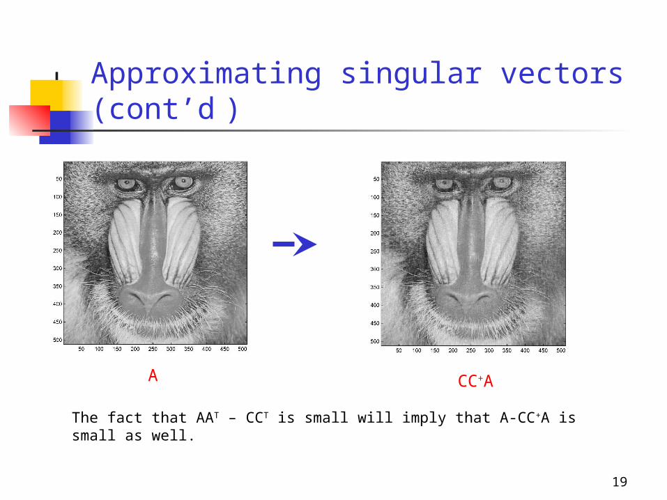
Title:C:\Petros\Image Processing\baboondet.epsCreator:MATLAB, The Mathworks, Inc.Preview:This EPS picture was not savedwith a preview included in it.Comment:This EPS picture will print to aPostScript printer, but not toother types of printers.
Original matrix Sampling (s=140 columns)
1. Sample s (=140) columns of the original matrix A and rescale them appropriately to form a 512-by-c matrix C.
2. Project A on CC+ and show that A-CC+A is “small”.
(C+ is the pseudoinverse of C)
Approximating singular vectors
18
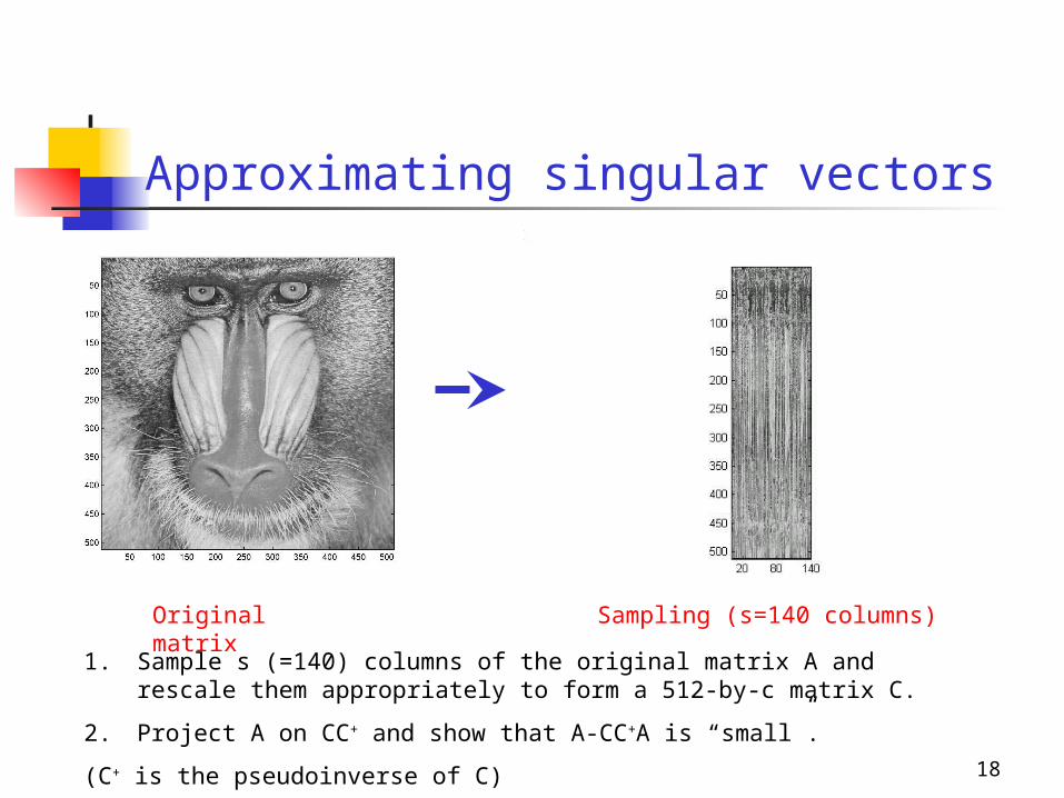
Title:C:\Petros\Image Processing\baboondet.epsCreator:MATLAB, The Mathworks, Inc.Preview:This EPS picture was not savedwith a preview included in it.Comment:This EPS picture will print to aPostScript printer, but not toother types of printers.
Original matrix Sampling (s=140 columns)
1. Sample s (=140) columns of the original matrix A and rescale them appropriately to form a 512-by-c matrix C.
2. Project A on CC+ and show that A-CC+A is “small”.
(C+ is the pseudoinverse of C)
Approximating singular vectors
19
Approximating singular vectors (cont’d )
Title:C:\Petros\Image Processing\baboondet.epsCreator:MATLAB, The Mathworks, Inc.Preview:This EPS picture was not savedwith a preview included in it.Comment:This EPS picture will print to aPostScript printer, but not toother types of printers.
A
The fact that AAT – CCT is small will imply that A-CC+A is small as well.
CC+A
20
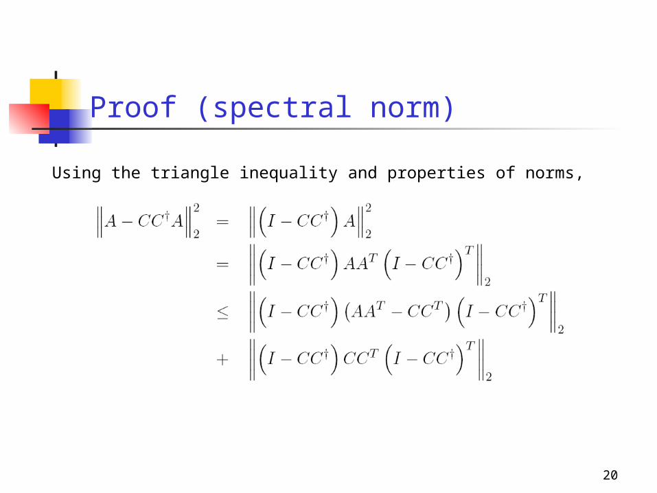
Proof (spectral norm)
Using the triangle inequality and properties of norms,
21
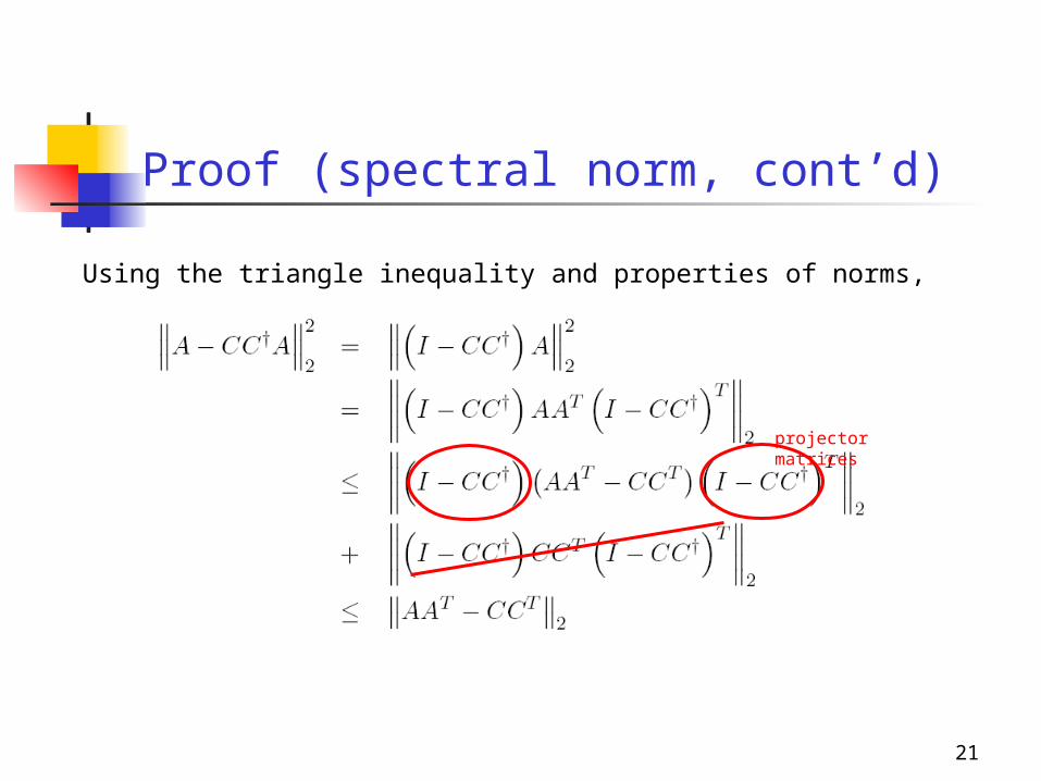
Proof (spectral norm, cont’d)
Using the triangle inequality and properties of norms,
projector matrices
22
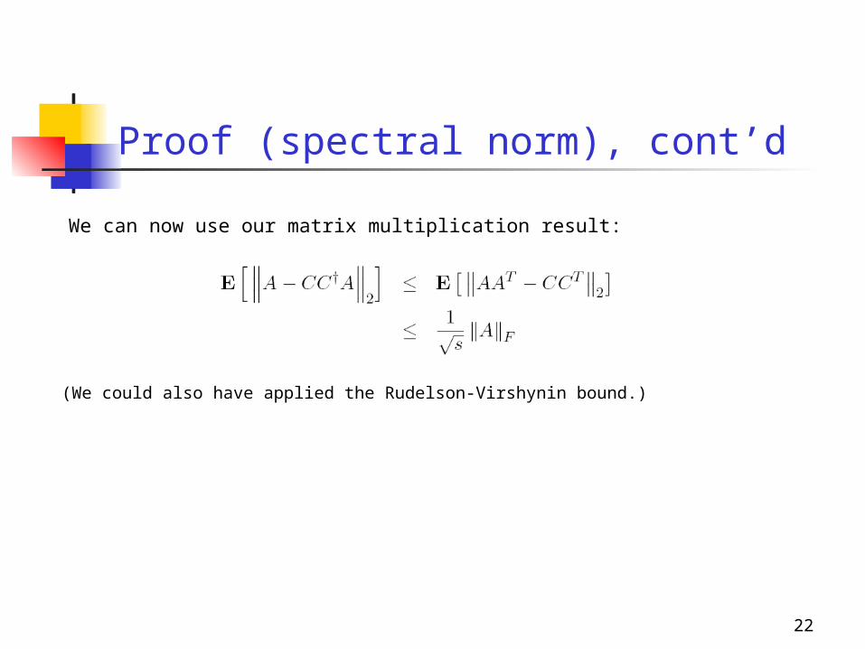
Proof (spectral norm), cont’d
We can now use our matrix multiplication result:
(We could also have applied the Rudelson-Virshynin bound.)

23
Is this a good bound?
Problem 1: If s = n, we still do not get zero error.
That’s because of sampling with replacement.
(We know how to analyze uniform sampling without replacement, but we have no bounds on non-uniform sampling without replacement.)
Problem 2: If A had rank exactly k, we would like a column selection procedure that drives the error down to zero when s=k.
This can be done deterministically simply by selecting k linearly independent columns.
Problem 3: If A had numerical rank k, we would like a bound that depends on the norm of A-Ak and not on the norm of A.
Such deterministic bounds exist when s=k and depend (roughly) on (k(n-k))1/2 ||A-Ak||2
24
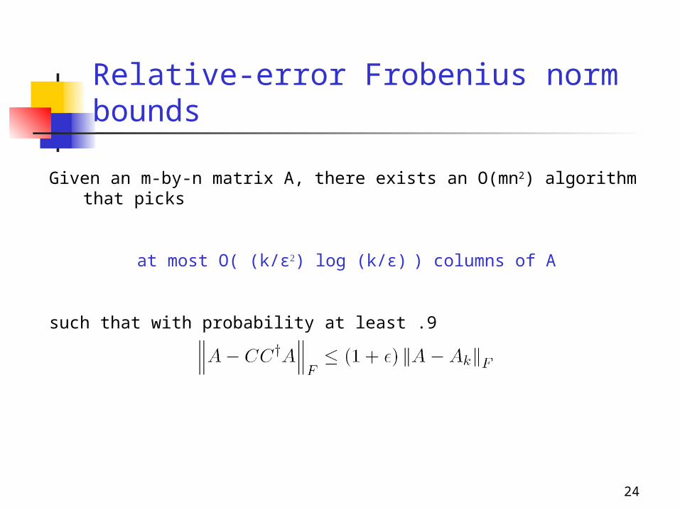
Relative-error Frobenius norm bounds
Given an m-by-n matrix A, there exists an O(mn2) algorithm that picks
at most O( (k/ε) log (k/ε) ) columns of A
such that with probability at least .9
25
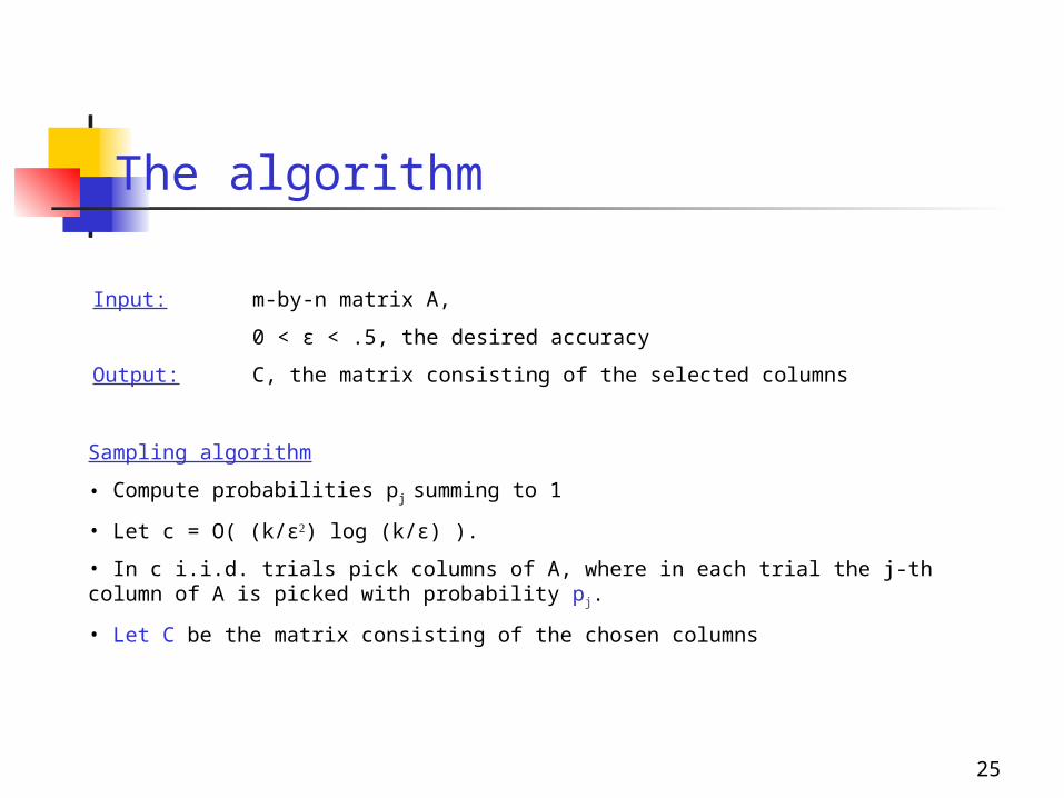
The algorithm
Sampling algorithm
• Compute probabilities pj summing to 1
• Let c = O( (k/ε) log (k/ε) ).
• In c i.i.d. trials pick columns of A, where in each trial the j-th column of A is picked with probability pj.
• Let C be the matrix consisting of the chosen columns
Input: m-by-n matrix A,
0 < ε < .5, the desired accuracy
Output: C, the matrix consisting of the selected columns
26
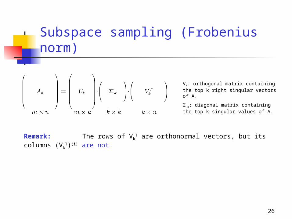
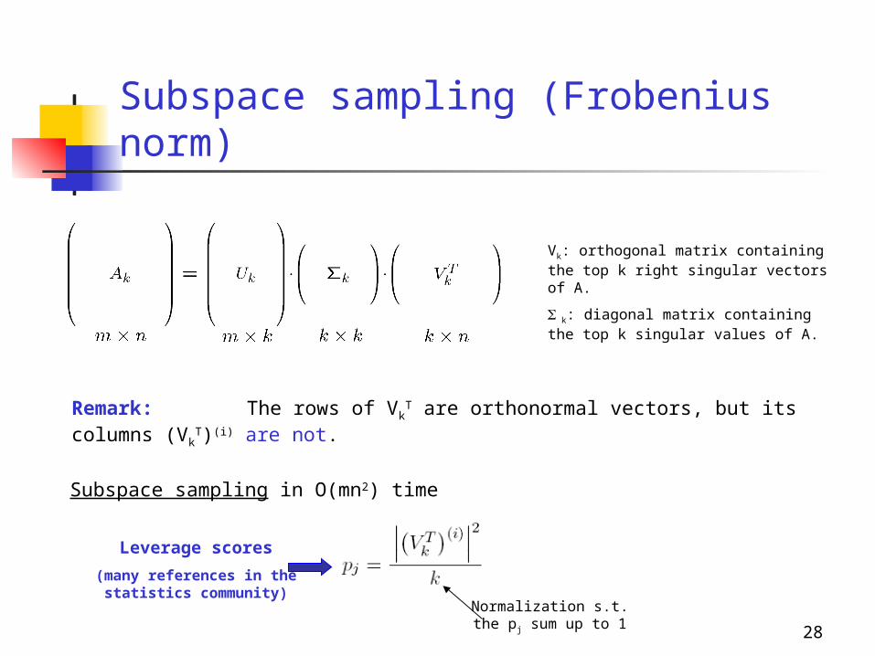
Subspace sampling (Frobenius norm)
Remark: The rows of VkT are orthonormal vectors, but its columns
(VkT)(i) are not.
Vk: orthogonal matrix containing the top k right singular vectors of A.
k: diagonal matrix containing the top k singular values of A.
27
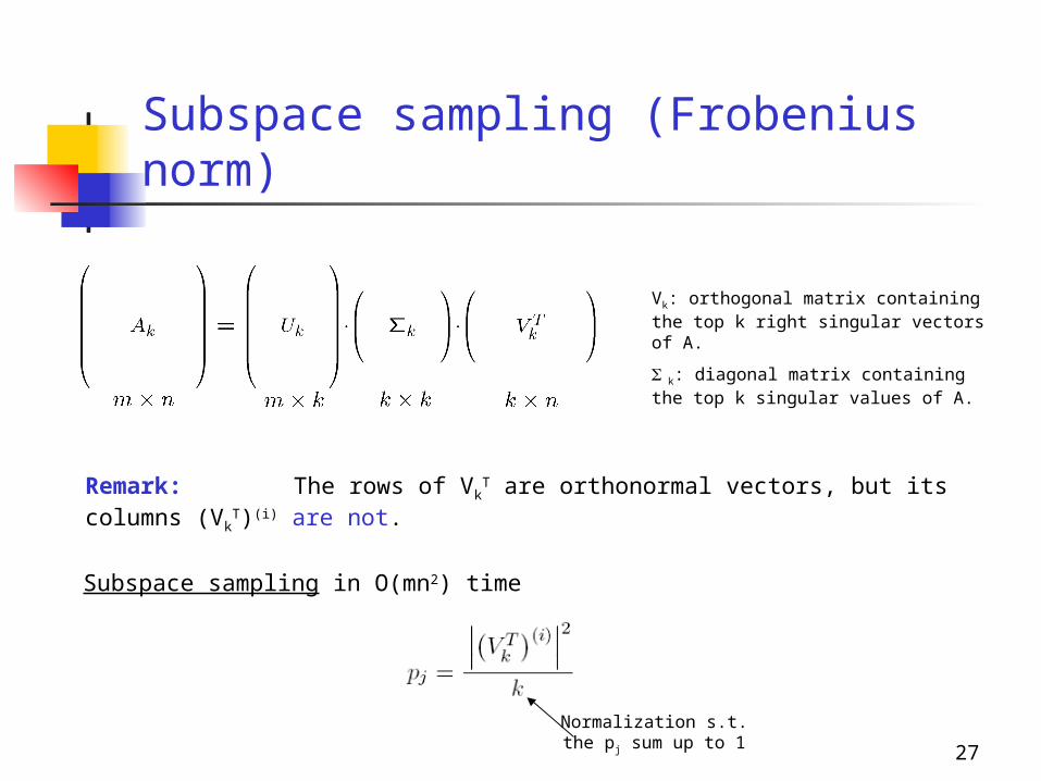
Subspace sampling (Frobenius norm)
Remark: The rows of VkT are orthonormal vectors, but its columns
(VkT)(i) are not.
Subspace sampling in O(mn2) time
Vk: orthogonal matrix containing the top k right singular vectors of A.
k: diagonal matrix containing the top k singular values of A.
Normalization s.t. the pj sum up to 1
28
Subspace sampling (Frobenius norm)
Remark: The rows of VkT are orthonormal vectors, but its columns
(VkT)(i) are not.
Subspace sampling in O(mn2) time
Vk: orthogonal matrix containing the top k right singular vectors of A.
k: diagonal matrix containing the top k singular values of A.
Normalization s.t. the pj sum up to 1
Leverage scores
(many references in the statistics community)
29
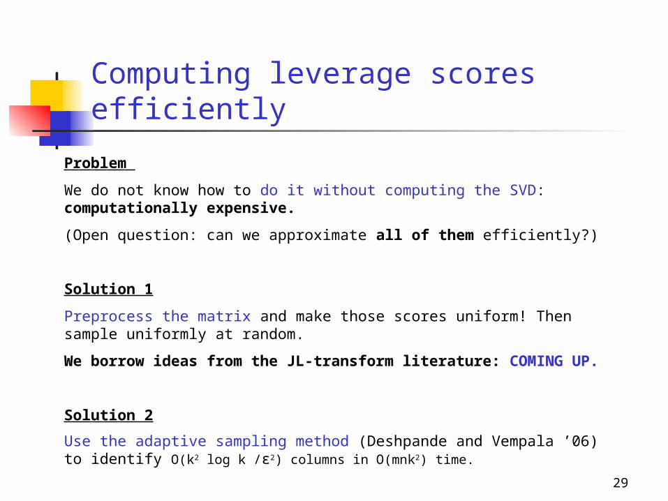
Computing leverage scores efficiently
Problem
We do not know how to do it without computing the SVD: computationally expensive.
(Open question: can we approximate all of them efficiently?)
Solution 1
Preprocess the matrix and make those scores uniform! Then sample uniformly at random.
We borrow ideas from the JL-transform literature: COMING UP.
Solution 2
Use the adaptive sampling method (Deshpande and Vempala ’06) to identify O(k2 log k /ε2) columns in O(mnk2) time.
30
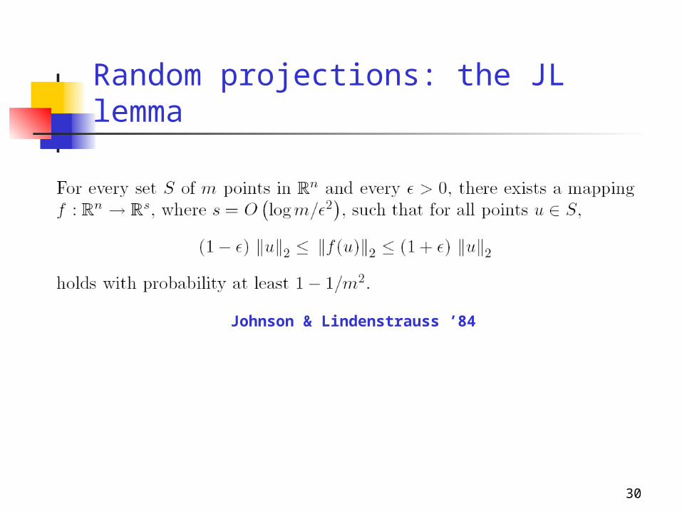
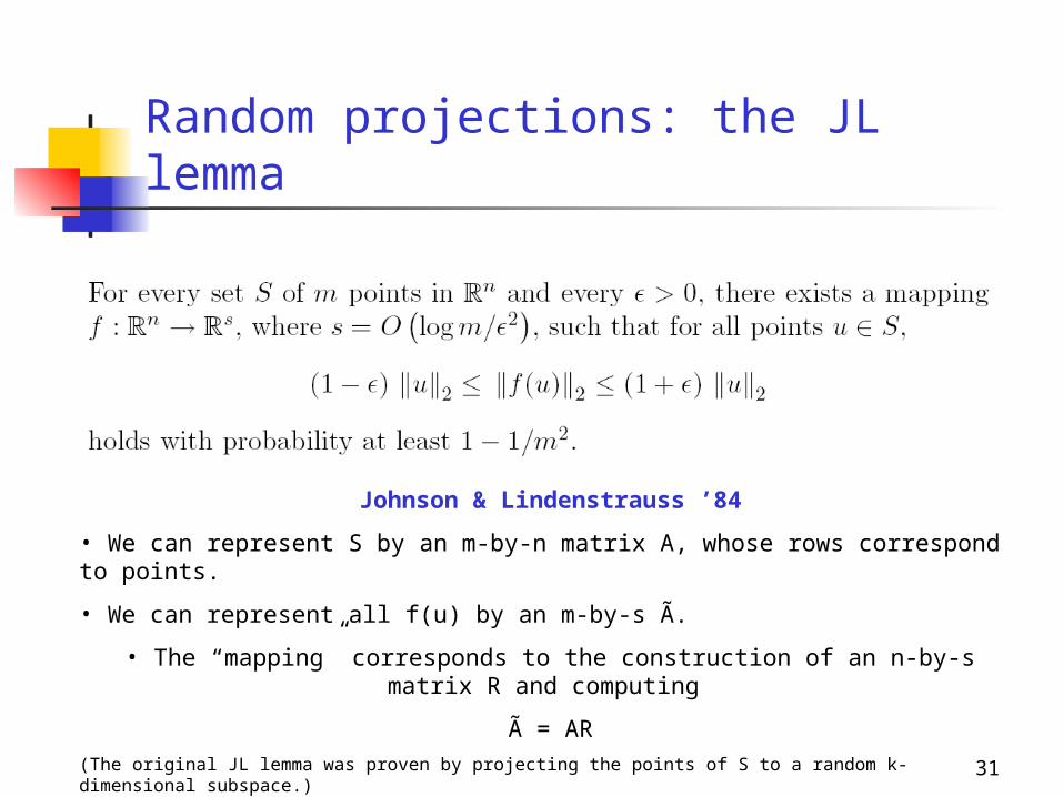
Random projections: the JL lemma
Johnson & Lindenstrauss ’84
31
Random projections: the JL lemma
Johnson & Lindenstrauss ’84
• We can represent S by an m-by-n matrix A, whose rows correspond to points.
• We can represent all f(u) by an m-by-s Ã.
• The “mapping” corresponds to the construction of an n-by-s matrix R and computing
à = AR(The original JL lemma was proven by projecting the points of S to a random k-dimensional subspace.)
32
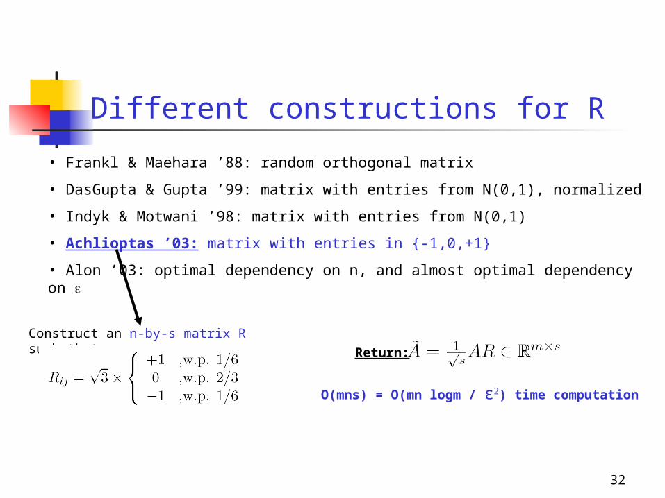
Different constructions for R
• Frankl & Maehara ’88: random orthogonal matrix
• DasGupta & Gupta ’99: matrix with entries from N(0,1), normalized
• Indyk & Motwani ’98: matrix with entries from N(0,1)
• Achlioptas ’03: matrix with entries in {-1,0,+1}
• Alon ’03: optimal dependency on n, and almost optimal dependency on
Construct an n-by-s matrix R such that: Return:
O(mns) = O(mn logm / ε) time computation
33
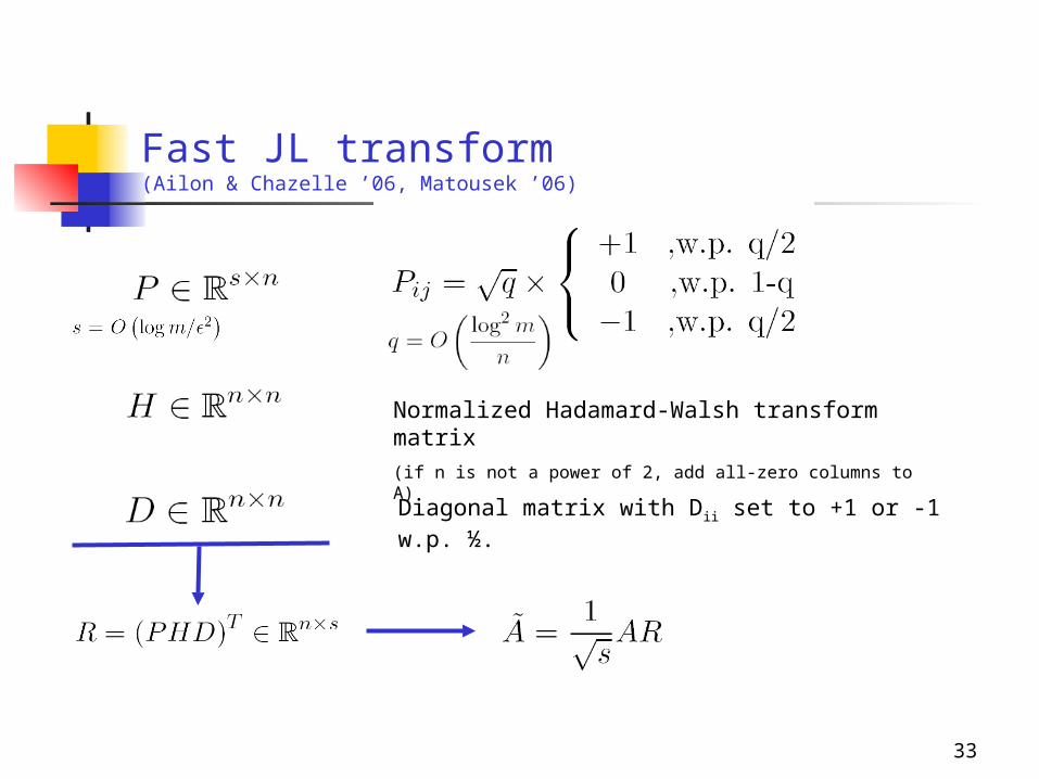
Fast JL transform(Ailon & Chazelle ’06, Matousek ’06)
Normalized Hadamard-Walsh transform matrix(if n is not a power of 2, add all-zero columns to A)
Diagonal matrix with Dii set to +1 or -1 w.p. ½.
34
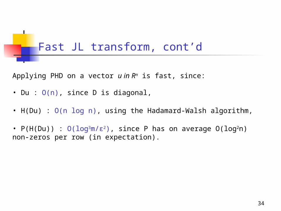
Applying PHD on a vector u in Rn is fast, since:
• Du : O(n), since D is diagonal,
• H(Du) : O(n log n), using the Hadamard-Walsh algorithm,
• P(H(Du)) : O(log3m/ε2), since P has on average O(log2n) non-zeros per row (in expectation).
Fast JL transform, cont’d
35
Back to approximating singular vectors
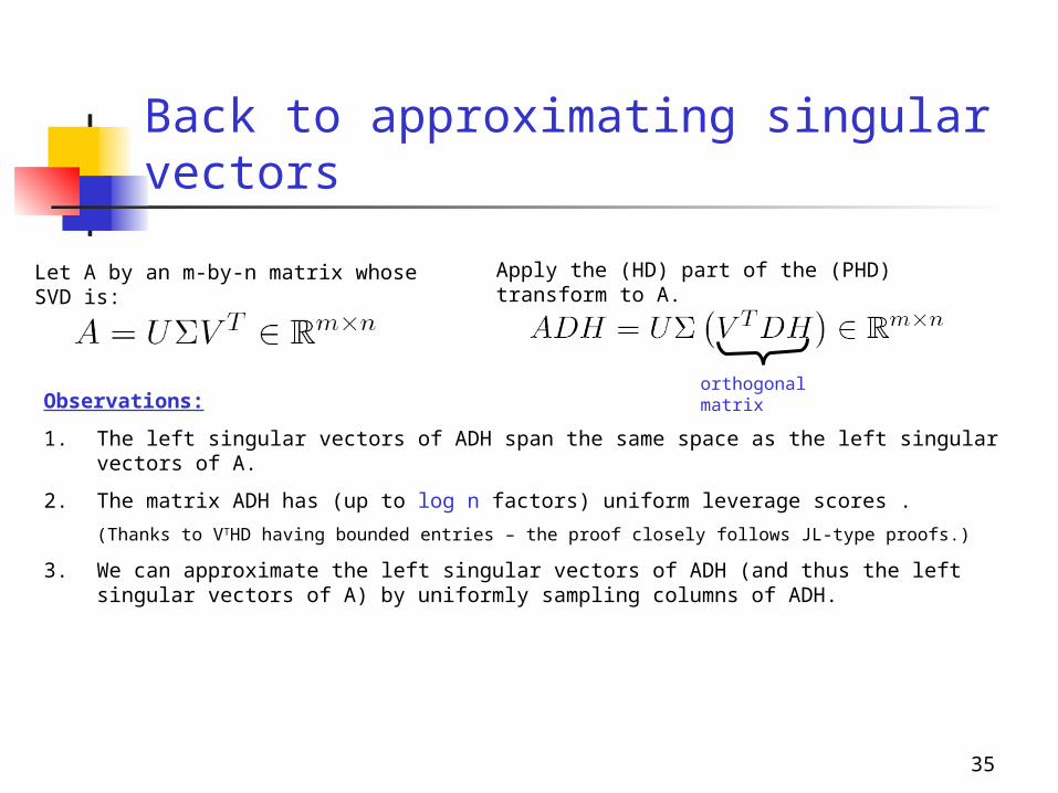
Let A by an m-by-n matrix whose SVD is:
Apply the (HD) part of the (PHD) transform to A.
Observations:
1. The left singular vectors of ADH span the same space as the left singular vectors of A.
2. The matrix ADH has (up to log n factors) uniform leverage scores .
(Thanks to VTHD having bounded entries – the proof closely follows JL-type proofs.)
3. We can approximate the left singular vectors of ADH (and thus the left singular vectors of A) by uniformly sampling columns of ADH.
orthogonal matrix

36
Back to approximating singular vectors
Let A by an m-by-n matrix whose SVD is:
Apply the (HD) part of the (PHD) transform to A.
Observations:
1. The left singular vectors of ADH span the same space as the left singular vectors of A.
2. The matrix ADH has (up to log n factors) uniform leverage scores .
(Thanks to VTHD having bounded entries – the proof closely follows JL-type proofs.)
3. We can approximate the left singular vectors of ADH (and thus the left singular vectors of A) by uniformly sampling columns of ADH.
4. The orthonormality of HD and a version of our relative-error Frobenius norm bound (involving approximately optimal sampling probabilities) suffice to show that (w.h.p.)
orthogonal matrix
37
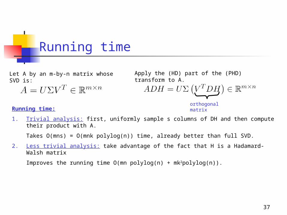
Running time
Let A by an m-by-n matrix whose SVD is:
Apply the (HD) part of the (PHD) transform to A.
Running time:
1. Trivial analysis: first, uniformly sample s columns of DH and then compute their product with A.
Takes O(mns) = O(mnk polylog(n)) time, already better than full SVD.
2. Less trivial analysis: take advantage of the fact that H is a Hadamard-Walsh matrix
Improves the running time O(mn polylog(n) + mk2polylog(n)).
orthogonal matrix
38
Conclusions
• Randomization and sampling can be used to solve problems that are massive and/or computationally expensive.
• By (carefully) sampling rows/columns/entries of a matrix, we can construct new sparse/smaller matrices that behave like the original matrix.
• By preprocessing the matrix using random projections, we can sample rows/ columns much less carefully (even uniformly at random) and still get nice “behavior”.