information retrieval & data mining: a linear algebraic perspective to access my web page:...
TRANSCRIPT

Information Retrieval & Data Mining: A Linear Algebraic Perspective
To access my web page:
Petros DrineasPetros Drineas
Rensselaer Polytechnic InstituteComputer Science Department
drineas

Modern data
Facts
Computers make it easy to collect and store data.
Costs of storage are very low and are dropping very fast.
(most laptops have a storage capacity of more than 100 GB …)
When it comes to storing data
The current policy typically is “store everything in case it is needed later” instead of deciding what could be deleted.

Data mining
Facts
Computers make it easy to collect and store data.
Costs of storage are very low and are dropping very fast.
(most laptops have a storage capacity of more than 100 GB …)
When it comes to storing data
The current policy typically is “store everything in case it is needed later” instead of deciding what could be deleted.
Data Mining
Extract useful information from the massive amount of available data.

About the tutorial
Tools
Introduce matrix algorithms and matrix decompositions for data mining and information retrieval applications.
Goal
Learn a model for the underlying “physical” system generating the dataset.

About the tutorial
Tools
Introduce matrix algorithms and matrix decompositions for data mining and information retrieval applications.
Goal
Learn a model for the underlying “physical” system generating the dataset.
algorithms mathematics
dataMath is necessary to design and analyze principled algorithmic
techniques to data-mine the massive datasets that have become ubiquitous
in scientific research.

Why linear (or multilinear) algebra?
Data are represented by matrices
Numerous modern datasets are in matrix form.
Data are represented by tensors
Data in the form of tensors (multi-mode arrays) are becoming very common in the data mining and information retrieval literature in the last few years.

Why linear (or multilinear) algebra?
Data are represented by matrices
Numerous modern datasets are in matrix form.
Data are represented by tensors
Data in the form of tensors (multi-mode arrays) are becoming very common in the data mining and information retrieval literature in the last few years.
Linear algebra (and numerical analysis) provide the fundamental mathematical and algorithmic tools to deal with matrix and tensor computations.
(This tutorial will focus on matrices; pointers to some tensor decompositions will be provided.)

Why matrix decompositions?
Matrix decompositions
(e.g., SVD, QR, SDD, CX and CUR, NMF, MMMF, etc.)
• They use the relationships between the available data in order to identify components of the underlying physical system generating the data.
• Some assumptions on the relationships between the underlying components are necessary.
• Very active area of research; some matrix decompositions are more than one century old, whereas others are very recent.

Overview
• Datasets in the form of matrices (and tensors)
• Matrix Decompositions
Singular Value Decomposition (SVD)Column-based Decompositions (CX, interpolative decomposition)CUR-type decompositionsNon-negative matrix factorizationSemi-Discrete Decomposition (SDD)Maximum-Margin Matrix Factorization (MMMF)Tensor decompositions
• Regression
Coreset constructionsFast algorithms for least-squares regression

Datasets in the form of matrices
We are given m objects and n features describing the objects.
(Each object has n numeric values describing it.)
Dataset
An m-by-n matrix A, Aij shows the “importance” of feature j for object i.
Every row of A represents an object.
Goal
We seek to understand the structure of the data, e.g., the underlying process generating the data.

Market basket matrices
Common representation for association rule mining.
m customer
s
n products
(e.g., milk, bread, wine, etc.)
A ij = quantity of j-th product purchased
by the i-th customer
Data mining tasks
- Find association rules E.g., customers who buy product x buy product y with probility 89%.
- Such rules are used to make item display decisions, advertising decisions, etc.

Social networks (e-mail graph)
Represents the email communications between groups of users.
n users
n users
A ij = number of emails exchanged
between users i and j during a certain time
period
Data mining tasks
- cluster the users
- identify “dense” networks of users (dense subgraphs)

Document-term matrices
A collection of documents is represented by an m-by-n matrix (bag-of-words model).
m documen
ts
n terms (words)
A ij = frequency of j-th term in i-th document
Data mining tasks
- Cluster or classify documents
- Find “nearest neighbors”
- Feature selection: find a subset of terms that (accurately) clusters or classifies documents.
Exam
ple late
r

Recommendation systems
The m-by-n matrix A represents m customers and n products.
customers
products
A ij = utility of j-th product to i-th
customer
Data mining task
Given a few samples from A, recommend high utility products to customers.

Microarray Data
Rows: genes (¼ 5,500)
Columns: 46 soft-issue tumour specimens
(different types of cancer, e.g., LIPO, LEIO, GIST, MFH, etc.)
Tasks:
Pick a subset of genes (if it exists) that suffices in order to identify the “cancer type” of a patient
gene
s
tumour specimens
Biology: microarray data
Nielsen et al., Lancet, 2002

Microarray Data
Rows: genes (¼ 5,500)
Columns: 46 soft-issue tumour specimens
(different types of cancer, e.g., LIPO, LEIO, GIST, MFH, etc.)
Tasks:
Pick a subset of genes (if it exists) that suffices in order to identify the “cancer type” of a patient
gene
s
tumour specimens
Biology: microarray data
Nielsen et al., Lancet, 2002Exa
mple la
ter

Single Nucleotide Polymorphisms: the most common type of genetic variation in the genome across different individuals.
They are known locations at the human genome where two alternate nucleotide bases (alleles) are observed (out of A, C, G, T).
SNPs
indiv
idu
als
… AG CT GT GG CT CC CC CC CC AG AG AG AG AG AA CT AA GG GG CC GG AG CG AC CC AA CC AA GG TT AG CT CG CG CG AT CT CT AG CT AG GG GT GA AG …
… GG TT TT GG TT CC CC CC CC GG AA AG AG AG AA CT AA GG GG CC GG AA GG AA CC AA CC AA GG TT AA TT GG GG GG TT TT CC GG TT GG GG TT GG AA …
… GG TT TT GG TT CC CC CC CC GG AA AG AG AA AG CT AA GG GG CC AG AG CG AC CC AA CC AA GG TT AG CT CG CG CG AT CT CT AG CT AG GG GT GA AG …
… GG TT TT GG TT CC CC CC CC GG AA AG AG AG AA CC GG AA CC CC AG GG CC AC CC AA CG AA GG TT AG CT CG CG CG AT CT CT AG CT AG GT GT GA AG …
… GG TT TT GG TT CC CC CC CC GG AA GG GG GG AA CT AA GG GG CT GG AA CC AC CG AA CC AA GG TT GG CC CG CG CG AT CT CT AG CT AG GG TT GG AA …
… GG TT TT GG TT CC CC CG CC AG AG AG AG AG AA CT AA GG GG CT GG AG CC CC CG AA CC AA GT TT AG CT CG CG CG AT CT CT AG CT AG GG TT GG AA …
… GG TT TT GG TT CC CC CC CC GG AA AG AG AG AA TT AA GG GG CC AG AG CG AA CC AA CG AA GG TT AA TT GG GG GG TT TT CC GG TT GG GT TT GG AA …
Matrices including hundreds of individuals and more than 300,000 SNPs are publicly available.
Task :split the individuals in different clusters depending on their ancestry, and
find a small subset of genetic markers that are “ancestry informative”.
Human genetics
Exam
ple late
r
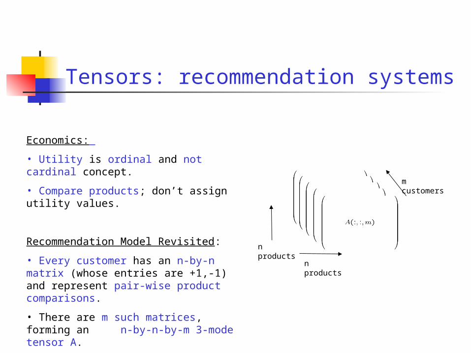
Tensors: recommendation systems
Economics:
• Utility is ordinal and not cardinal concept.
• Compare products; don’t assign utility values.
Recommendation Model Revisited:
• Every customer has an n-by-n matrix (whose entries are +1,-1) and represent pair-wise product comparisons.
• There are m such matrices, forming an n-by-n-by-m 3-mode tensor A.
n products
n products
m customers

Tensors: hyperspectral images
Task:
Identify and analyze regions of significance in the images.
Spectrally resolved images may be viewed as a tensor.
ca. 500 pixels
ca. 500 pixels
128 frequencies

Overview
• Datasets in the form of matrices (and tensors)
• Matrix Decompositions
Singular Value Decomposition (SVD)Column-based Decompositions (CX, interpolative decomposition)CUR-type decompositionsNon-negative matrix factorizationSemi-Discrete Decomposition (SDD)Maximum-Margin Matrix Factorization (MMMF)Tensor decompositions
• Regression
Coreset constructionsFast algorithms for least-squares regression
x

The Singular Value Decomposition (SVD)
feature 1
fea
ture
2
Object x
Object d
(d,x)
Recall: data matrices have m rows (one for each object) and n columns (one for each feature).
Matrix rows: points (vectors) in a Euclidean space,
e.g., given 2 objects (x & d), each described with respect to two features, we get a 2-by-2 matrix.
Two objects are “close” if the angle between their corresponding vectors is small.

4.0 4.5 5.0 5.5 6.02
3
4
5
SVD, intuition
Let the blue circles represent m data points in a 2-D Euclidean space.
Then, the SVD of the m-by-2 matrix of the data will return …
1st (right) singular vector
1st (right) singular vector:
direction of maximal variance,
2nd (right) singular vector
2nd (right) singular vector:
direction of maximal variance, after removing the projection of the data along the first singular vector.

4.0 4.5 5.0 5.5 6.02
3
4
5
1st (right) singular vector
2nd (right) singular vector
Singular values
1: measures how much of the data variance is explained by the first singular vector.
2: measures how much of the data variance is explained by the second singular vector.1
2
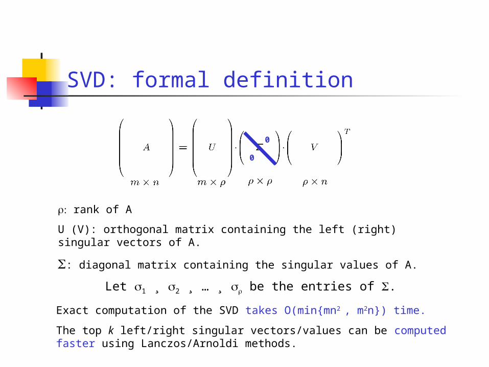
SVD: formal definition
rank of A
U (V): orthogonal matrix containing the left (right) singular vectors of A.
: diagonal matrix containing the singular values of A.
Let 1 ¸ 2 ¸ … ¸ be the entries of .
Exact computation of the SVD takes O(min{mn2 , m2n}) time.
The top k left/right singular vectors/values can be computed faster using Lanczos/Arnoldi methods.
0
0

A VTU=
objects
features
significant
noisenois
e noise
signifi
cant
sig.
=
Rank-k approximations via the SVD

Rank-k approximations (Ak)
Uk (Vk): orthogonal matrix containing the top k left (right) singular vectors of A.
k: diagonal matrix containing the top k singular values of A.

PCA and SVD
feature 1
fea
ture
2
Object x
Object d
(d,x)
Principal Components Analysis (PCA) essentially amounts to the computation of the Singular Value Decomposition (SVD) of a covariance matrix.
SVD is the algorithmic tool behind MultiDimensional Scaling (MDS) and Factor Analysis.
SVD is “the Rolls-Royce and the Swiss Army Knife of Numerical Linear Algebra.”*
*Dianne O’Leary, MMDS ’06

Ak as an optimization problem
Given , it is easy to find X from standard least squares.
However, the fact that we can find the optimal is intriguing!
Frobenius norm:
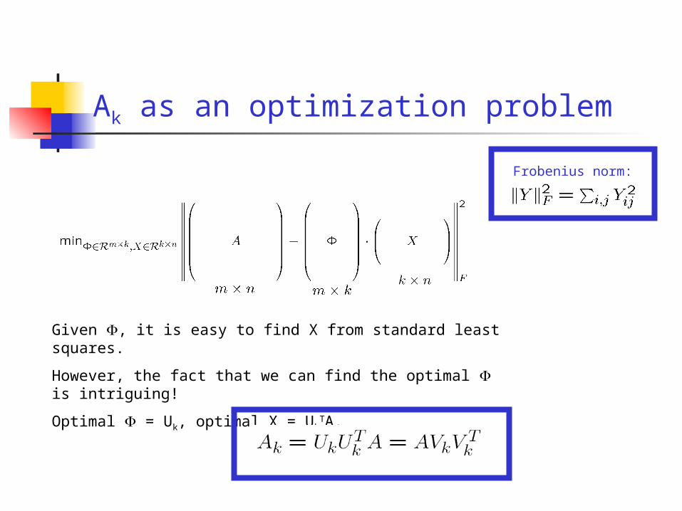
Ak as an optimization problem
Given , it is easy to find X from standard least squares.
However, the fact that we can find the optimal is intriguing!
Optimal = Uk, optimal X = UkTA.
Frobenius norm:
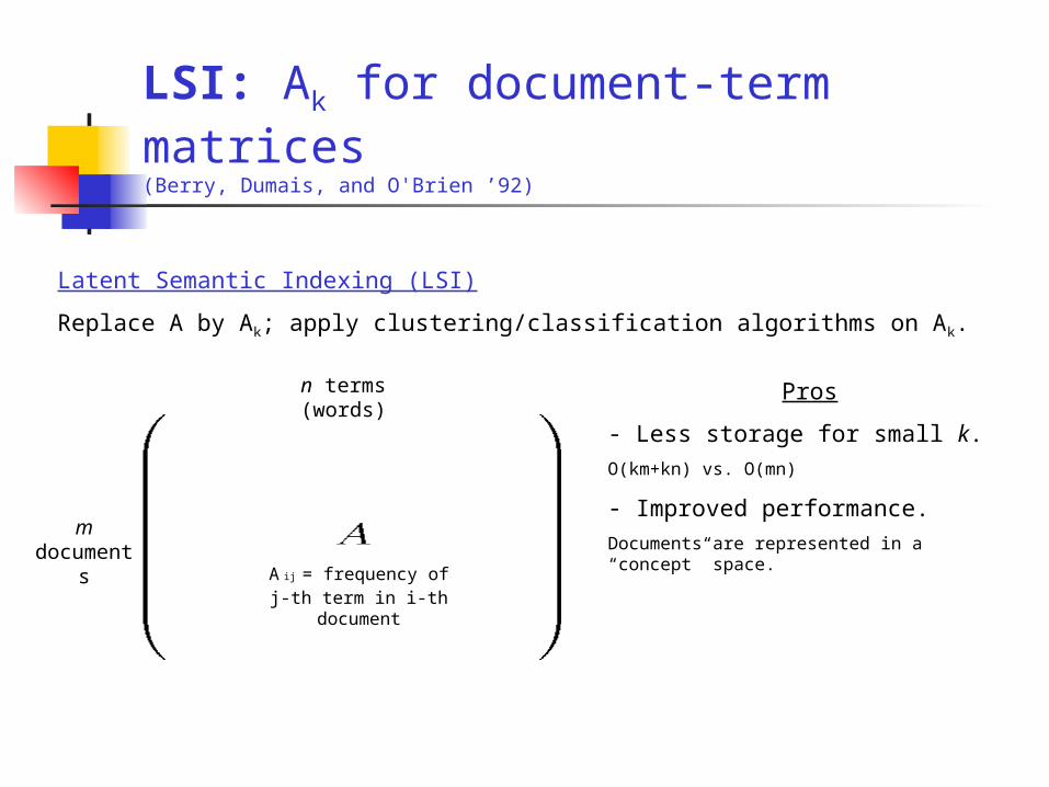
LSI: Ak for document-term matrices(Berry, Dumais, and O'Brien ’92)
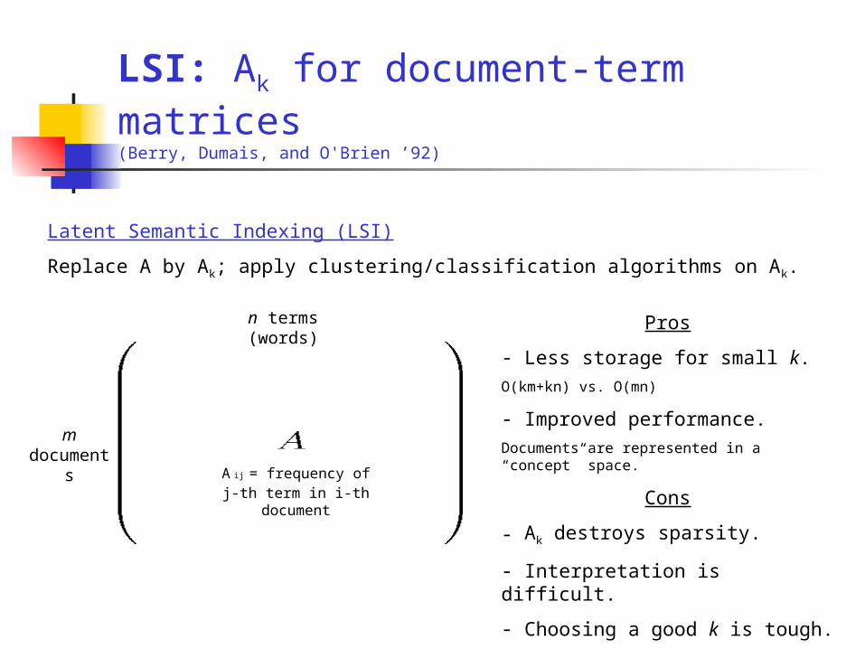
Latent Semantic Indexing (LSI)
Replace A by Ak; apply clustering/classification algorithms on Ak.
m documen
ts
n terms (words)
A ij = frequency of j-th term in i-th document
Pros
- Less storage for small k.O(km+kn) vs. O(mn)
- Improved performance.Documents are represented in a “concept” space.
Latent Semantic Indexing (LSI)
Replace A by Ak; apply clustering/classification algorithms on Ak.
m documen
ts
n terms (words)
A ij = frequency of j-th term in i-th document
Pros
- Less storage for small k.O(km+kn) vs. O(mn)
- Improved performance.Documents are represented in a “concept” space.
Cons
- Ak destroys sparsity.
- Interpretation is difficult.
- Choosing a good k is tough.
LSI: Ak for document-term matrices(Berry, Dumais, and O'Brien ’92)

Ak and k-means clustering(Drineas, Frieze, Kannan, Vempala, and Vinay ’99)
k-means clustering
A standard objective function that measures cluster quality.
(Often denotes an iterative algorithm that attempts to optimize the k-means objective function.)
k-means objective
Input: set of m points in Rn, positive integer k
Output: a partition of the m points to k clusters
Partition the m points to k clusters in order to minimize the sum of the squared Euclidean distances from each point to its cluster centroid.

k-means, cont’d
We seek to split the input points in 5 clusters.

k-means, cont’d
We seek to split the input points in 5 clusters.
The cluster centroid is the “average” of all the points in the cluster.

k-means: a matrix formulation
Let A be the m-by-n matrix representing m points in Rn. Then, we seek to
X is a special “cluster membership” matrix: Xij denotes if the i-th point belongs to the j-th cluster.

k-means: a matrix formulation
Let A be the m-by-n matrix representing m points in Rn. Then, we seek to
X is a special “cluster membership” matrix: Xij denotes if the i-th point belongs to the j-th cluster.
poin
ts
clusters • Columns of X are normalized to have unit length.
(We divide each column by the square root of the number of points in the cluster.)
• Every row of X has at most one non-zero element.
(Each element belongs to at most one cluster.)
• X is an orthogonal matrix, i.e., XTX = I.

SVD and k-means
If we only require that X is an orthogonal matrix and remove the condition on the number of non-zero entries per row of X, then
is easy to minimize! The solution is X = Uk.

SVD and k-means
If we only require that X is an orthogonal matrix and remove the condition on the number of non-zero entries per row of X, then
is easy to minimize! The solution is X = Uk.Using SVD to solve k-means
• We can get a 2-approximation algorithm for k-means.
(Drineas, Frieze, Kannan, Vempala, and Vinay ’99, ’04)
• We can get heuristic schemes to assign points to clusters.
(Zha, He, Ding, Simon, and Gu ’01)
• There exist PTAS (based on random projections) for the k-means problem.
(Ostrovsky and Rabani ’00, ’02)
• Deeper connections between SVD and clustering in Kannan, Vempala, and Vetta ’00, ’04.

Ak and Kleinberg’s HITS algorithm(Kleinberg ’98, ’99)
Hypertext Induced Topic Selection (HITS)
A link analysis algorithm that rates Web pages for their authority and hub scores.
Authority score: an estimate of the value of the content of the page.
Hub score: an estimate of the value of the links from this page to other pages.
These values can be used to rank Web search results.

Ak and Kleinberg’s HITS algorithm
Hypertext Induced Topic Selection (HITS)
A link analysis algorithm that rates Web pages for their authority and hub scores.
Authority score: an estimate of the value of the content of the page.
Hub score: an estimate of the value of the links from this page to other pages.
These values can be used to rank Web search results.
Authority: a page that is pointed to by many pages with high hub scores.
Hub: a page pointing to many pages that are good authorities.
Recursive definition; notice that each node has two scores.

Ak and Kleinberg’s HITS algorithm
Phase 1:
Given a query term (e.g., “jaguar”), find all pages containing the query term (root set).
Expand the resulting graph by one move forward and backward (base set).

Ak and Kleinberg’s HITS algorithm
Phase 2:
Let A be the adjacency matrix of the (directed) graph of the base set.
Let h , a 2 Rn be the vectors of hub (authority) scores.
Then, h = Aa and a = ATh
h = AATh and a = ATAa.

Ak and Kleinberg’s HITS algorithm
Phase 2:
Let A be the adjacency matrix of the (directed) graph of the base set.
Let h , a 2 Rn be the vectors of hub (authority) scores.
Then, h = Aa and a = ATh
h = AATh and a = ATAa.
Thus, the top left (right) singular vector of A corresponds to hub (authority) scores.
What about the rest?
They provide a natural way to extract additional densely linked collections of hubs and authorities from the base set.
See the “jaguar” example in Kleinberg ’99.

Microarray Data(Nielsen et al., Lancet, 2002)
Columns: genes (¼ 5,500)
Rows: 32 patients, three different cancer types (GIST, LEIO, SynSarc)
SVD example: microarray data
genes

Microarray Data
Applying k-means with k=3 in this 3D space results to 3 misclassifications.
Applying k-means with k=3 but retaining 4 PCs results to one misclassification.
Can we find actual genes (as opposed to eigengenes) that achieve similar results?
SVD example: microarray data

SVD example: ancestry-informative SNPs
Single Nucleotide Polymorphisms: the most common type of genetic variation in the genome across different individuals.
They are known locations at the human genome where two alternate nucleotide bases (alleles) are observed (out of A, C, G, T).
SNPs
indiv
idu
als
… AG CT GT GG CT CC CC CC CC AG AG AG AG AG AA CT AA GG GG CC GG AG CG AC CC AA CC AA GG TT AG CT CG CG CG AT CT CT AG CT AG GG GT GA AG …
… GG TT TT GG TT CC CC CC CC GG AA AG AG AG AA CT AA GG GG CC GG AA GG AA CC AA CC AA GG TT AA TT GG GG GG TT TT CC GG TT GG GG TT GG AA …
… GG TT TT GG TT CC CC CC CC GG AA AG AG AA AG CT AA GG GG CC AG AG CG AC CC AA CC AA GG TT AG CT CG CG CG AT CT CT AG CT AG GG GT GA AG …
… GG TT TT GG TT CC CC CC CC GG AA AG AG AG AA CC GG AA CC CC AG GG CC AC CC AA CG AA GG TT AG CT CG CG CG AT CT CT AG CT AG GT GT GA AG …
… GG TT TT GG TT CC CC CC CC GG AA GG GG GG AA CT AA GG GG CT GG AA CC AC CG AA CC AA GG TT GG CC CG CG CG AT CT CT AG CT AG GG TT GG AA …
… GG TT TT GG TT CC CC CG CC AG AG AG AG AG AA CT AA GG GG CT GG AG CC CC CG AA CC AA GT TT AG CT CG CG CG AT CT CT AG CT AG GG TT GG AA …
… GG TT TT GG TT CC CC CC CC GG AA AG AG AG AA TT AA GG GG CC AG AG CG AA CC AA CG AA GG TT AA TT GG GG GG TT TT CC GG TT GG GT TT GG AA …
There are ¼ 10 million SNPs in the human genome, so this table could have ~10 million columns.

Focus at a specific locus and assay the observed nucleotide bases (alleles).
SNP: exactly two alternate alleles appear.
Two copies of a chromosome (father,
mother)

SNPs
indiv
idu
als
… AG CT GT GG CT CC CC CC CC AG AG AG AG AG AA CT AA GG GG CC GG AG CG AC CC AA CC AA GG TT AG CT CG CG CG AT CT CT AG CT AG GG GT GA AG …
… GG TT TT GG TT CC CC CC CC GG AA AG AG AG AA CT AA GG GG CC GG AA GG AA CC AA CC AA GG TT AA TT GG GG GG TT TT CC GG TT GG GG TT GG AA …
… GG TT TT GG TT CC CC CC CC GG AA AG AG AA AG CT AA GG GG CC AG AG CG AC CC AA CC AA GG TT AG CT CG CG CG AT CT CT AG CT AG GG GT GA AG …
… GG TT TT GG TT CC CC CC CC GG AA AG AG AG AA CC GG AA CC CC AG GG CC AC CC AA CG AA GG TT AG CT CG CG CG AT CT CT AG CT AG GT GT GA AG …
… GG TT TT GG TT CC CC CC CC GG AA GG GG GG AA CT AA GG GG CT GG AA CC AC CG AA CC AA GG TT GG CC CG CG CG AT CT CT AG CT AG GG TT GG AA …
… GG TT TT GG TT CC CC CG CC AG AG AG AG AG AA CT AA GG GG CT GG AG CC CC CG AA CC AA GT TT AG CT CG CG CG AT CT CT AG CT AG GG TT GG AA …
… GG TT TT GG TT CC CC CC CC GG AA AG AG AG AA TT AA GG GG CC AG AG CG AA CC AA CG AA GG TT AA TT GG GG GG TT TT CC GG TT GG GT TT GG AA …
Focus at a specific locus and assay the observed alleles.
SNP: exactly two alternate alleles appear.
Two copies of a chromosome (father,
mother)
C T
An individual could be:
- Heterozygotic (in our study, CT = TC)

SNPs
indiv
idu
als
… AG CT GT GG CT CC CC CC CC AG AG AG AG AG AA CT AA GG GG CC GG AG CG AC CC AA CC AA GG TT AG CT CG CG CG AT CT CT AG CT AG GG GT GA AG …
… GG TT TT GG TT CC CC CC CC GG AA AG AG AG AA CT AA GG GG CC GG AA GG AA CC AA CC AA GG TT AA TT GG GG GG TT TT CC GG TT GG GG TT GG AA …
… GG TT TT GG TT CC CC CC CC GG AA AG AG AA AG CT AA GG GG CC AG AG CG AC CC AA CC AA GG TT AG CT CG CG CG AT CT CT AG CT AG GG GT GA AG …
… GG TT TT GG TT CC CC CC CC GG AA AG AG AG AA CC GG AA CC CC AG GG CC AC CC AA CG AA GG TT AG CT CG CG CG AT CT CT AG CT AG GT GT GA AG …
… GG TT TT GG TT CC CC CC CC GG AA GG GG GG AA CT AA GG GG CT GG AA CC AC CG AA CC AA GG TT GG CC CG CG CG AT CT CT AG CT AG GG TT GG AA …
… GG TT TT GG TT CC CC CG CC AG AG AG AG AG AA CT AA GG GG CT GG AG CC CC CG AA CC AA GT TT AG CT CG CG CG AT CT CT AG CT AG GG TT GG AA …
… GG TT TT GG TT CC CC CC CC GG AA AG AG AG AA TT AA GG GG CC AG AG CG AA CC AA CG AA GG TT AA TT GG GG GG TT TT CC GG TT GG GT TT GG AA …
C C
Focus at a specific locus and assay the observed alleles.
SNP: exactly two alternate alleles appear.
Two copies of a chromosome (father,
mother)An individual could be:
- Heterozygotic (in our study, CT = TC)
- Homozygotic at the first allele, e.g., C

SNPs
indiv
idu
als
… AG CT GT GG CT CC CC CC CC AG AG AG AG AG AA CT AA GG GG CC GG AG CG AC CC AA CC AA GG TT AG CT CG CG CG AT CT CT AG CT AG GG GT GA AG …
… GG TT TT GG TT CC CC CC CC GG AA AG AG AG AA CT AA GG GG CC GG AA GG AA CC AA CC AA GG TT AA TT GG GG GG TT TT CC GG TT GG GG TT GG AA …
… GG TT TT GG TT CC CC CC CC GG AA AG AG AA AG CT AA GG GG CC AG AG CG AC CC AA CC AA GG TT AG CT CG CG CG AT CT CT AG CT AG GG GT GA AG …
… GG TT TT GG TT CC CC CC CC GG AA AG AG AG AA CC GG AA CC CC AG GG CC AC CC AA CG AA GG TT AG CT CG CG CG AT CT CT AG CT AG GT GT GA AG …
… GG TT TT GG TT CC CC CC CC GG AA GG GG GG AA CT AA GG GG CT GG AA CC AC CG AA CC AA GG TT GG CC CG CG CG AT CT CT AG CT AG GG TT GG AA …
… GG TT TT GG TT CC CC CG CC AG AG AG AG AG AA CT AA GG GG CT GG AG CC CC CG AA CC AA GT TT AG CT CG CG CG AT CT CT AG CT AG GG TT GG AA …
… GG TT TT GG TT CC CC CC CC GG AA AG AG AG AA TT AA GG GG CC AG AG CG AA CC AA CG AA GG TT AA TT GG GG GG TT TT CC GG TT GG GT TT GG AA …
T T
Focus at a specific locus and assay the observed alleles.
SNP: exactly two alternate alleles appear.
Two copies of a chromosome (father,
mother)An individual could be:
- Heterozygotic (in our study, CT = TC)
- Homozygotic at the first allele, e.g., C
- Homozygotic at the second allele, e.g., T
Encode as 0
Encode as +1
Encode as -1

(a) Why are SNPs really important?
Association studies:
Locating causative genes for common complex disorders (e.g., diabetes, heart disease, etc.) is based on identifying association between affection status and known SNPs.
No prior knowledge about the function of the gene(s) or the etiology of the disorder is necessary.
The subsequent investigation of candidate genes that are in physical proximity with the associated SNPs is the first step towards understanding the etiological “pathway” of a disorder and designing a drug.

(b) Why are SNPs really important?
Among different populations (eg., European, Asian, African, etc.), different patterns of SNP allele frequencies or SNP correlations are often observed.
Understanding such differences is crucial in order to develop the “next generation” of drugs that will be “population specific” (eventually “genome specific”) and not just “disease specific”.

The HapMap project
Also, funding from pharmaceutical companies, NSF, the Department of Justice*, etc.
• Mapping the whole genome sequence of a single individual is very expensive.
• Mapping all the SNPs is also quite expensive, but the costs are dropping fast.
HapMap project (~$130,000,000 funding from NIH and other sources):
Map approx. 4 million SNPs for 270 individuals from 4 different populations (YRI, CEU, CHB, JPT), in order to create a “genetic map” to be used by researchers.
*Is it possible to identify the ethnicity of a suspect from his DNA?

CHB and JPT
Let A be the 90£2.7 million matrix of the CHB and JPT population in HapMap.
• Run SVD (PCA) on A, keep the two (left) singular vectors, and plot the results.
• Run a (naïve, e.g., k-means) clustering algorithm to split the data points in two clusters.Paschou, Ziv, Burchard, Mahoney, and Drineas, to appear in PLOS Genetics ’07(data from E. Ziv and E. Burchard, UCSF)
Paschou, Mahoney, Javed, Kidd, Pakstis, Gu, Kidd, and Drineas, Genome Research ’07(data from K. Kidd, Yale University)


EigenSNPs can not be assayed…
Not altogether satisfactory: the (top two left) singular vectors are linear combinations of all SNPs, and – of course – can not be assayed!
Can we find actual SNPs that capture the information in the (top two left) singular vectors?
(E.g., spanning the same subspace …)
Will get back to this later …

Overview
• Datasets in the form of matrices (and tensors)
• Matrix Decompositions
Singular Value Decomposition (SVD)Column-based Decompositions (CX, interpolative decomposition)CUR-type decompositionsNon-negative matrix factorizationSemi-Discrete Decomposition (SDD)Maximum-Margin Matrix Factorization (MMMF)Tensor decompositions
• Regression
Coreset constructionsFast algorithms for least-squares regression
x
x

CX decomposition
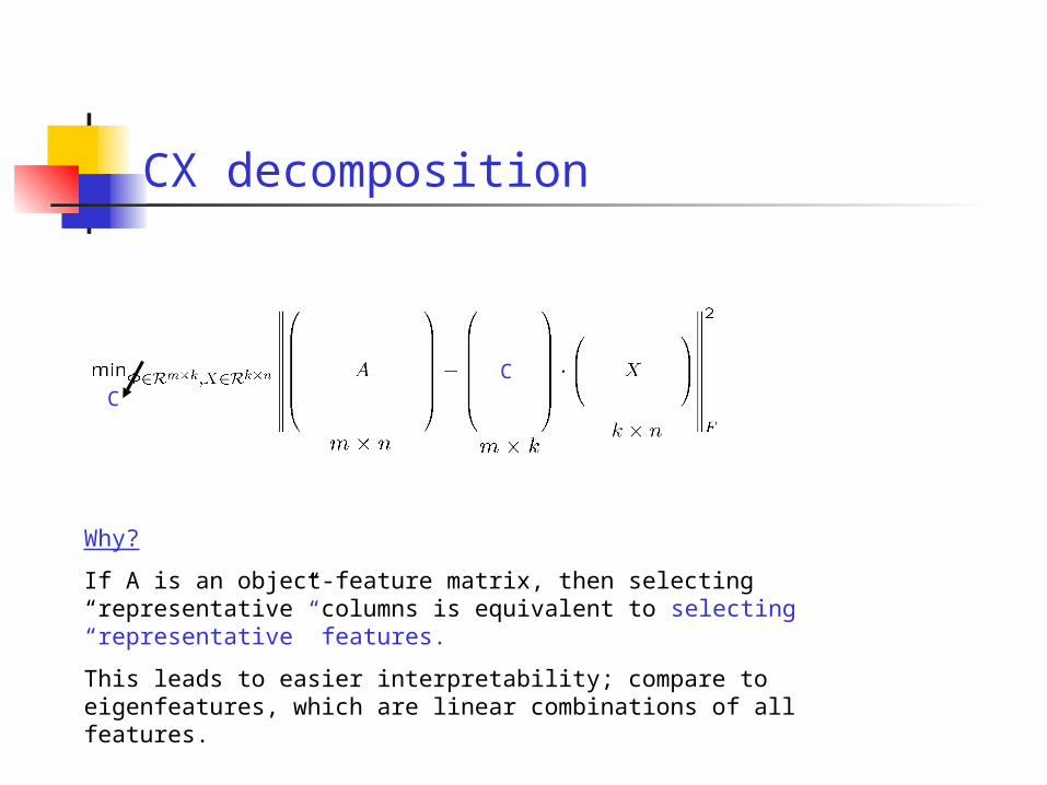
Constrain to contain exactly k columns of A.
Notation: replace by C(olumns).
Easy to prove that optimal X = C+A. (C+ is the Moore-Penrose pseudoinverse of C.)
Also called “interpolative approximation”.(some extra conditions on the elements of X are required…)
CC
CX decomposition
Why?
If A is an object-feature matrix, then selecting “representative” columns is equivalent to selecting “representative” features.
This leads to easier interpretability; compare to eigenfeatures, which are linear combinations of all features.
CC
Column Subset Selection problem (CSS)
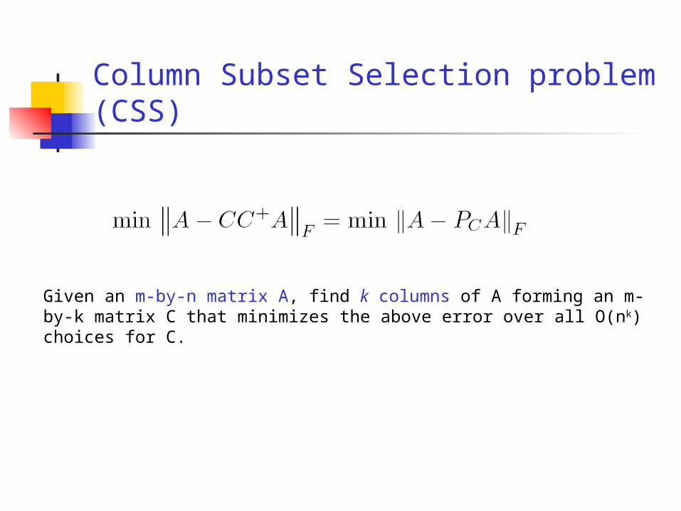
Given an m-by-n matrix A, find k columns of A forming an m-by-k matrix C that minimizes the above error over all O(nk) choices for C.

Column Subset Selection problem (CSS)
Given an m-by-n matrix A, find k columns of A forming an m-by-k matrix C that minimizes the above error over all O(nk) choices for C.
C+: pseudoinverse of C, easily computed via the SVD of C.(If C = U VT, then C+ = V -1 UT.)
PC = CC+ is the projector matrix on the subspace spanned by the columns of C.

Column Subset Selection problem (CSS)
Given an m-by-n matrix A, find k columns of A forming an m-by-k matrix C that minimizes the above error over all O(nk) choices for C.
PC = CC+ is the projector matrix on the subspace spanned by the columns of C.
Complexity of the problem? O(nkmn) trivially works; NP-hard if k grows as a function of n. (NP-hardness in Civril & Magdon-Ismail ’07)

Spectral norm
Given an m-by-n matrix A, find k columns of A forming an m-by-k matrix C such that
is minimized over all O(nk) possible choices for C.
Remarks:
1. PCA is the projection of A on the subspace spanned by the columns of C.
2. The spectral or 2-norm of an m-by-n matrix X is

A lower bound for the CSS problem
For any m-by-k matrix C consisting of at most k columns of A
Remarks:
1. This is also true if we replace the spectral norm by the Frobenius norm.
2. This is a – potentially – weak lower bound.
Ak

Prior work: numerical linear algebra
Numerical Linear Algebra algorithms for CSS
1. Deterministic, typically greedy approaches.
2. Deep connection with the Rank Revealing QR factorization.
3. Strongest results so far (spectral norm): in O(mn2) time
some function p(k,n)

Prior work: numerical linear algebra
Numerical Linear Algebra algorithms for CSS
1. Deterministic, typically greedy approaches.
2. Deep connection with the Rank Revealing QR factorization.
3. Strongest results so far (Frobenius norm): in O(nk) time

Working on p(k,n): 1965 – today
Prior work: theoretical computer science
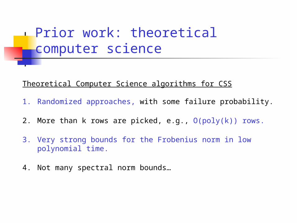
Theoretical Computer Science algorithms for CSS
1. Randomized approaches, with some failure probability.
2. More than k rows are picked, e.g., O(poly(k)) rows.
3. Very strong bounds for the Frobenius norm in low polynomial time.
4. Not many spectral norm bounds…

The strongest Frobenius norm bound
Given an m-by-n matrix A, there exists an O(mn2) algorithm that picks
at most O( k log k / 2 ) columns of A
such that with probability at least 1-10-20

The CX algorithm
CX algorithm
• Compute probabilities pj summing to 1
• Let c = O(k log k / 2)
• For each j = 1,2,…,n, pick the j-th column of A with probability min{1,cpj}
• Let C be the matrix consisting of the chosen columns
(C has – in expectation – at most c columns)
Input: m-by-n matrix A,
0 < < 1, the desired accuracy
Output: C, the matrix consisting of the selected columns

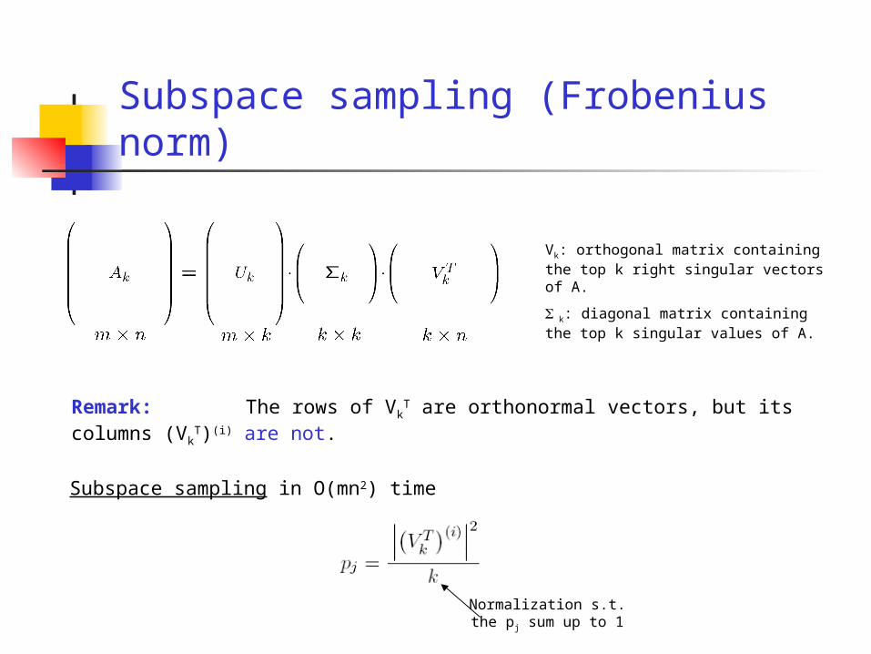
Subspace sampling (Frobenius norm)
Remark: The rows of VkT are orthonormal vectors, but its columns
(VkT)(i) are not.
Vk: orthogonal matrix containing the top k right singular vectors of A.
k: diagonal matrix containing the top k singular values of A.
Subspace sampling (Frobenius norm)
Remark: The rows of VkT are orthonormal vectors, but its columns
(VkT)(i) are not.
Subspace sampling in O(mn2) time
Vk: orthogonal matrix containing the top k right singular vectors of A.
k: diagonal matrix containing the top k singular values of A.
Normalization s.t. the pj sum up to 1

Prior work in TCS
Drineas, Mahoney, and Muthukrishnan 2005
• O(mn2) time, O(k2/2) columns
Drineas, Mahoney, and Muthukrishnan 2006
• O(mn2) time, O(k log k/2) columns
Deshpande and Vempala 2006
• O(mnk2) time and O(k2 log k/2) columns
• They also prove the existence of k columns of A forming a matrix C, such that
• Compare to prior best existence result:

Open problems
Design:
• Faster algorithms (next slide)
• Algorithms that achieve better approximation guarantees (a hybrid approach)

Prior work spanning NLA and TCS
Woolfe, Liberty, Rohklin, and Tygert 2007
(also Martinsson, Rohklin, and Tygert 2006)
• O(mn logk) time, k columns, same spectral norm bounds as prior work
• Beautiful application of the Fast Johnson-Lindenstrauss transform of Ailon-Chazelle

A hybrid approach(Boutsidis, Mahoney, and Drineas ’07)
Given an m-by-n matrix A (assume m ¸ n for simplicity):
• (Randomized phase) Run a randomized algorithm to pick c = O(k logk) columns.
• (Deterministic phase) Run a deterministic algorithm on the above columns* to pick exactly k columns of A and form an m-by-k matrix C. * Not so simple …

Given an m-by-n matrix A (assume m ¸ n for simplicity):
• (Randomized phase) Run a randomized algorithm to pick c = O(k logk) columns.
• (Deterministic phase) Run a deterministic algorithm on the above columns* to pick exactly k columns of A and form an m-by-k matrix C.
Our algorithm runs in O(mn2) and satisfies, with probability at least 1-10-20,
* Not so simple …
A hybrid approach(Boutsidis, Mahoney, and Drineas ’07)
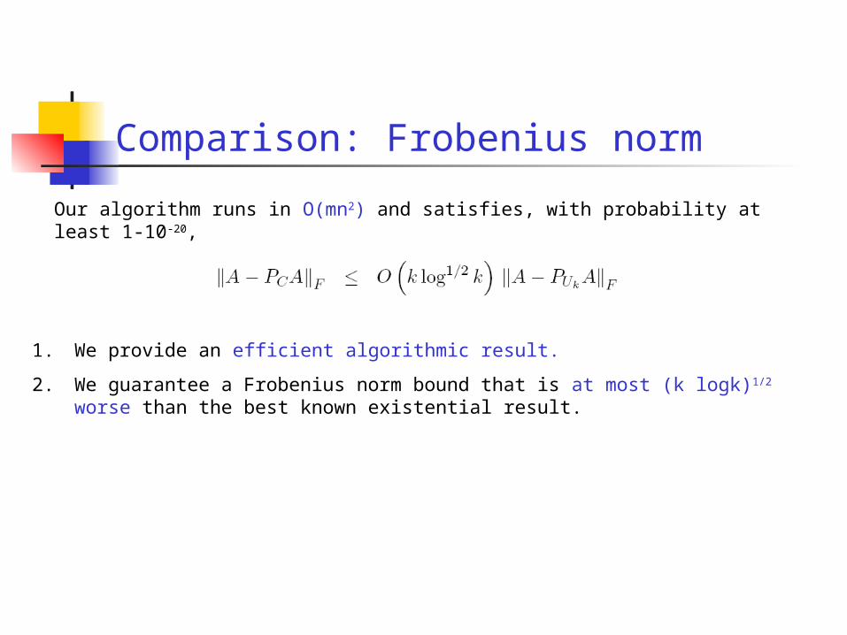
Comparison: Frobenius norm
1. We provide an efficient algorithmic result.
2. We guarantee a Frobenius norm bound that is at most (k logk)1/2 worse than the best known existential result.
Our algorithm runs in O(mn2) and satisfies, with probability at least 1-10-20,

Comparison: spectral norm
1. Our running time is comparable with NLA algorithms for this problem.
2. Our spectral norm bound grows as a function of (n-k)1/4 instead of (n-k)1/2!
3. Do notice that with respect to k our bound is k1/4log1/2k worse than previous work.
4. To the best of our knowledge, our result is the first asymptotic improvement of the work of Gu & Eisenstat 1996.
Our algorithm runs in O(mn2) and satisfies, with probability at least 1-10-20,

Randomized phase: O(k log k) columns
Randomized phase: c = O(k logk)
• Compute probabilities pj summing to 1
• For each j = 1,2,…,n, pick the j-th column of A with probability min{1,cpj}
• Let C be the matrix consisting of the chosen columns
(C has – in expectation – at most c columns)

Subspace sampling
Remark: We need more elaborate subspace sampling probabilities than previous work.
Subspace sampling in O(mn2) time
Vk: orthogonal matrix containing the top k right singular vectors of A.
k: diagonal matrix containing the top k singular values of A.
Normalization s.t. the pj sum up to 1

Deterministic phase: k columns
Deterministic phase
• Let S1 be the set of indices of the columns selected by the randomized phase.
• Let (VkT)S1 denote the set of columns of Vk
T with indices in S1,
(An extra technicality is that the columns of (VkT)S1 must be rescaled …)
• Run a deterministic NLA algorithm on (VkT)S1 to select exactly k columns.
(Any algorithm with p(k,n) = k1/2(n-k)1/2 will do.)
• Let S2 be the set of indices of the selected columns (the cardinality of S2 is exactly k).
• Return AS2 (the columns of A corresponding to indices in S2) as the final output.

Back to SNPs: CHB and JPT
Let A be the 90£2.7 million matrix of the CHB and JPT population in HapMap.
Can we find actual SNPs that capture the information in the top two left singular vectors?

Results
• Essentially as good as the best existing metric (informativeness).
• However, our metric is unsupervised!
(Informativeness is supervised: it essentially identifies SNPs that are correlated with population membership, given such membership information).
• The fact that we can select ancestry informative SNPs in an unsupervised manner based on PCA is novel, and seems interesting.
Number of SNPs
Misclassifications
40 (c = 400) 6
50 (c = 500) 5
60 (c = 600) 3
70 (c = 700) 1
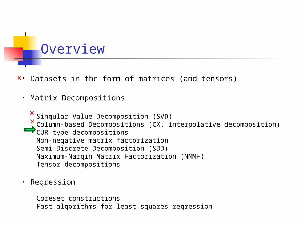
Overview
• Datasets in the form of matrices (and tensors)
• Matrix Decompositions
Singular Value Decomposition (SVD)Column-based Decompositions (CX, interpolative decomposition)CUR-type decompositionsNon-negative matrix factorizationSemi-Discrete Decomposition (SDD)Maximum-Margin Matrix Factorization (MMMF)Tensor decompositions
• Regression
Coreset constructionsFast algorithms for least-squares regression
x
xx

CUR-type decompositions
O(1) columnsO(1) rows
Carefully chosen U
Goal: make (some norm) of A-CUR small.
For any matrix A, we can find C, U and R such that the norm of A – CUR is almost equal to the norm of A-Ak.
This might lead to a better understanding of the data.

Theorem: relative error CUR(Drineas, Mahoney, & Muthukrishnan ’06, ’07)
For any k, O(mn2) time suffices to construct C, U, and R s.t.
holds with probability at least 1-, by picking
O( k log k log(1/) / 2 ) columns, and
O( k log2k log(1/) / 6 ) rows.

From SVD to CUR
Exploit structural properties of CUR to analyze data:
Instead of reifying the Principal Components:
• Use PCA (a.k.a. SVD) to find how many Principal Components are needed to “explain” the data.
• Run CUR and pick columns/rows instead of eigen-columns and eigen-rows!
• Assign meaning to actual columns/rows of the matrix! Much more intuitive! Sparse!
A CUR-type decomposition needs O(min{mn2, m2n}) time.
m objects
n features

CUR decompositions: a summary
G.W. Stewart(Num. Math. ’99, TR ’04 )
C: variant of the QR algorithmR: variant of the QR algorithmU: minimizes ||A-CUR||F
No a priori boundsSolid experimental performance
Goreinov, Tyrtyshnikov, and Zamarashkin
(LAA ’97, Cont. Math. ’01)
C: columns that span max volumeU: W+
R: rows that span max volume
Existential resultError bounds depend on ||W+||2
Spectral norm bounds!
Williams and Seeger(NIPS ’01)
C: uniformly at randomU: W+
R: uniformly at random
Experimental evaluationA is assumed PSDConnections to Nystrom method
Drineas, Kannan, and Mahoney(SODA ’03, ’04)
C: w.r.t. column lengthsU: in linear/constant timeR: w.r.t. row lengths
Randomized algorithmProvable, a priori, boundsExplicit dependency on A – Ak
Drineas, Mahoney, and Muthu(’05, ’06)
C: depends on singular vectors of A. U: (almost) W+
R: depends on singular vectors of C
(1+) approximation to A – Ak
Computable in SVDk(A) time.

Data applications of CUR
CMD factorization(Sun, Xie, Zhang, and Faloutsos ’07, best paper award in SIAM Conference on Data Mining ‘07)
A CUR-type decomposition that avoids duplicate rows/columns that might appear in some earlier versions of CUR-type decomposition.
Many interesting applications to large network datasets, DBLP, etc.; extensions to tensors.
Fast computation of Fourier Integral Operators (Demanet, Candes, and Ying ’06)
Application in seismology imaging data (PBytes of data can be generated…)
The problem boils down to solving integral equations, i.e., matrix equations after discretization.
CUR-type structures appear; uniform sampling seems to work well in practice.

Overview
• Datasets in the form of matrices (and tensors)
• Matrix Decompositions
Singular Value Decomposition (SVD)Column-based Decompositions (CX, interpolative decomposition)CUR-type decompositionsNon-negative matrix factorizationSemi-Discrete Decomposition (SDD)Maximum-Margin Matrix Factorization (MMMF)Tensor decompositions
• Regression
Coreset constructionsFast algorithms for least-squares regression
x
xxx

Decompositions that respect the data
Non-negative matrix factorization
(Lee and Seung ’00)
Assume that the Aij are non-negative for all i,j.
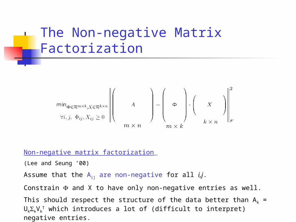
The Non-negative Matrix Factorization
Non-negative matrix factorization
(Lee and Seung ’00)
Assume that the Aij are non-negative for all i,j.
Constrain and X to have only non-negative entries as well.
This should respect the structure of the data better than Ak = UkkVkT which
introduces a lot of (difficult to interpret) negative entries.

The Non-negative Matrix Factorization
It has been extensively applied to:
1. Image mining (Lee and Seung ’00)
2. Enron email collection (Berry and Brown ’05)
3. Other text mining tasks (Berry and Plemmons ’04)
Algorithms for NMF:
1. Multiplicative updage rules (Lee and Seung ’00, Hoyer ’02)
2. Gradient descent (Hoyer ’04, Berry and Plemmons ’04)
3. Alternating least squares (dating back to Paatero ’94)

Algorithmic challenges for NMF
Algorithmic challenges for the NMF:
1. NMF (as stated above) is convex given or X, but not if both are unknown.
2. No unique solution: many matrices and X that minimize the error.
3. Other optimization objectives could be chosen (e.g., spectral norm, etc.)
4. NMF becomes harder if sparsity constraints are included (e.g., X has a small number of non-zeros).
5. For the multiplicative update rules there exists some theory proving that they converge to a fixed point; this might be a local optimum or a saddle point.
6. Little theory is known for the other algorithms.

Overview
• Datasets in the form of matrices (and tensors)
• Matrix Decompositions
Singular Value Decomposition (SVD)Column-based Decompositions (CX, interpolative decomposition)CUR-type decompositionsNon-negative matrix factorizationSemi-Discrete Decomposition (SDD)Maximum-Margin Matrix Factorization (MMMF)Tensor decompositions
• Regression
Coreset constructionsFast algorithms for least-squares regression
x
xxxx

SemiDiscrete Decomposition (SDD)
Xk DkYk
TASDD
Dk: diagonal matrix
Xk, Yk: all entries are in {-1,0,+1}
SDD identifies regions of the matrix that have homogeneous density.

SemiDiscrete Decomposition (SDD)
SDD looks for blocks of similar height towers and similar depth holes: “bump hunting”.
Applications include image compression and text mining.
O’Leary and Peleg ’83, Kolda and O’Leary ’98, ’00, O’Leary and Roth ’06
The figures are from D. Skillkorn’s book on Data Mining with Matrix Decompositions.

Overview
• Datasets in the form of matrices (and tensors)
• Matrix Decompositions
Singular Value Decomposition (SVD)Column-based Decompositions (CX, interpolative decomposition)CUR-type decompositionsNon-negative matrix factorizationSemi-Discrete Decomposition (SDD)Maximum-Margin Matrix Factorization (MMMF)Tensor decompositions
• Regression
Coreset constructionsFast algorithms for least-squares regression
x
xxxxx

Collaborative Filtering and MMMF
User ratings for movies
Goal: predict unrated movies (?)

Collaborative Filtering and MMMF
User ratings for movies
Goal: predict unrated movies (?)
Maximum Margin Matrix Factorization (MMMF)
A novel, semi-definite programming based matrix decomposition that seems to perform very well in real data, including the Netflix challenge.
Srebro, Rennie, and Jaakkola ’04, Rennie and Srebro ’05
Some pictures are from Srebro’s presentation in NIPS ’04.

A linear factor model

A linear factor model
T
User biases for different movie
attributes

All users
T
(Possible) solution to collaborative filtering: fit a rank (exactly) k matrix X to Y.
Fully observed Y X is the best rank k approximation to Y.
Azar, Fiat, Karlin, McSherry, and Saia ’01, Drineas, Kerenidis, and Raghavan ’02

Imputing the missing entries via SVD(Achlioptas and McSherry ’01, ’06)
Reconstruction Algorithm
• Compute the SVD of the matrix filling in the missing entries with zeros.
• Some rescaling prior to computing the SVD is necessary, e.g., multiply by 1/(fraction of observed entries).
• Keep the resulting top k principal components.
Under assumptions on the “quality” of the observed entries, reconstruction accuracy bounds may be proven.
The error bounds scale with the Frobenius norm of the matrix.

A convex formulation
MMMF
• Focus on §1 rankings (for simplicity).
• Fit a prediction matrix X = UVT to the observations.
T

A convex formulation
MMMF
• Focus on §1 rankings (for simplicity).
• Fit a prediction matrix X = UVT to the observations.
Objectives (CONVEX!)
• Minimize the total number of mismatches between the observed data and the predicted data.
• Keep the trace norm of X small.
T

A convex formulation
MMMF
• Focus on §1 rankings (for simplicity).
• Fit a prediction matrix X = UVT to the observations.
Objectives (CONVEX!)
• Minimize the total number of mismatches between the observed data and the predicted data.
• Keep the trace norm of X small.
T

MMMF and SDP
MMMF
This may be formulated as a semi-definite program, and thus may be solved efficiently.
T

Bounding the factor contribution
MMMF
Instead of a hard rank constraint (non-convex), a softer constraint is introduced.
The total number of contributing factors (number of columns/rows in U/VT) is unbounded, but their total contribution is bounded.
T

Overview
• Datasets in the form of matrices (and tensors)
• Matrix Decompositions
Singular Value Decomposition (SVD)Column-based Decompositions (CX, interpolative decomposition)CUR-type decompositionsNon-negative matrix factorizationSemi-Discrete Decomposition (SDD)Maximum-Margin Matrix Factorization (MMMF)Tensor decompositions
• Regression
Coreset constructionsFast algorithms for least-squares regression
x
xxxxxx

Tensors
Tensors appear both in Math and CS.
• Connections to complexity theory (i.e., matrix multiplication complexity)
• Data Set applications (i.e., Independent Component Analysis, higher order statistics, etc.)
Also, many practical applications, e.g., Medical Imaging, Hyperspectral Imaging, video, Psychology, Chemometrics, etc.
However, there does not exist a definition of tensor rank (and associated tensor SVD) with the – nice – properties found in the matrix case.

Tensor rank
A definition of tensor rank
Given a tensor
find the minimum number of rank one tensors into it can be decomposed.
only weak bounds are known tensor rank depends on the underlying ring of scalars computing it is NP-hard successive rank one approxi-imations are no good
agrees with matrices for d=2 related to computing bilinear forms and algebraic complexity theory.
BUT
outer product

Tensors decompositions
Many tensor decompositions “matricize” the tensor
1. PARAFAC, Tucker, Higher-Order SVD, DEDICOM, etc.
2. Most are computed via iterative algorithms (e.g., alternating least squares).
Given create the “unfolded” matrix
“unfold”

Useful links on tensor decompositions
• Workshop on Algorithms for Modern Massive Data Sets (MMDS) ’06
http://www.stanford.edu/group/mmds/
Check the tutorial by Lek-Heng Lim on tensor decompositions.
• Tutorial by Faloutsos, Kolda, and Sun in SIAM Data Mining Conference ’07
• Tammy Kolda’s web page
http://csmr.ca.sandia.gov/~tgkolda/

Overview
• Datasets in the form of matrices (and tensors)
• Matrix Decompositions
Singular Value Decomposition (SVD)Column-based Decompositions (CX, interpolative decomposition)CUR-type decompositionsNon-negative matrix factorizationSemi-Discrete Decomposition (SDD)Maximum-Margin Matrix Factorization (MMMF)Tensor decompositions
• Regression
Coreset constructionsFast algorithms for least-squares regression
x
xxxxxxx
x

Problem definition and motivation
In many applications (e.g., statistical data analysis and scientific computation), one has n observations of the form:
A is an n x d “design matrix” (n >> d):
In matrix-vector notation,
Model y(t) (unknown) as a linear combination of d basis functions:

Least-norm approximation problems
Recall a linear measurement model:
In order to estimate x, solve:

Application: data analysis in science
• First application: Astronomy
Predicting the orbit of the asteroid Ceres (in 1801!).
Gauss (1809) -- see also Legendre (1805) and Adrain (1808).
First application of “least squares optimization” and runs in O(nd2) time!
• Data analysis: Fit parameters of a biological, chemical, economical, physical (astronomical), social, internet, etc. model to experimental data.

Norms of common interest
Least-squares approximation:
Chebyshev or mini-max approximation:
Sum of absolute residuals approximation:
Let y = b and define the residual:

Lp norms and their unit balls
Recall the Lp norm for :
Some inequality relationships include:

Lp regression problems
We are interested in over-constrained Lp regression problems, n >> d.
Typically, there is no x such that Ax = b.
Want to find the “best” x such that Ax ≈ b.
Lp regression problems are convex programs (or better).
There exist poly-time algorithms.
We want to solve them faster.
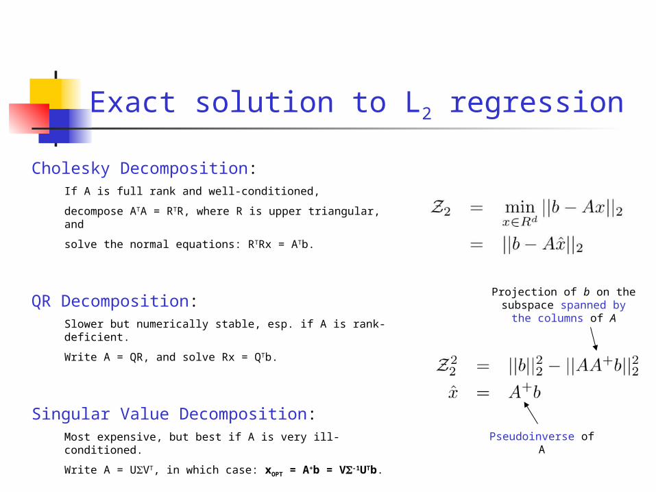
Exact solution to L2 regression
Cholesky Decomposition: If A is full rank and well-conditioned,
decompose ATA = RTR, where R is upper triangular, and
solve the normal equations: RTRx = ATb.
QR Decomposition: Slower but numerically stable, esp. if A is rank-deficient.
Write A = QR, and solve Rx = QTb.
Singular Value Decomposition:Most expensive, but best if A is very ill-conditioned.
Write A = UVT, in which case: xOPT = A+b = V-1UTb.
Complexity is O(nd2) , but constant factors differ.
Projection of b on the subspace spanned by the
columns of A
Pseudoinverse of A

Questions …
Approximation algorithms:
Can we approximately solve Lp regression faster than “exact” methods?
Core-sets (or induced sub-problems):
Can we find a small set of constraints such that solving the Lp regression on those constraints gives an approximation to the original problem?

Randomized algorithms for Lp regression
Alg. 1 p=2 Sampling (core-set)
(1+)-approx
O(nd2) Drineas, Mahoney, and Muthu ’06, ’07
Alg. 2 p=2 Projection (no core-set)
(1+)-approx
O(nd logd) Sarlos ’06 Drineas, Mahoney, Muthu, and Sarlos ’07
Alg. 3 p [1,∞) Sampling (core-set)
(1+)-approx
O(nd5) +o(“exact”)
DasGupta, Drineas, Harb, Kumar, & Mahoney ’07
Note: Clarkson ’05 gets a (1+)-approximation for L1 regression in O*(d3.5/4) time.
He preprocessed [A,b] to make it “well-rounded” or “well-conditioned” and then sampled.

Algorithm 1: Sampling for L2 regression
Algorithm
1. Fix a set of probabilities pi, i=1…n, summing up to 1.
2. Pick the i-th row of A and the i-th element of b with probability
min {1, rpi},
and rescale both by (1/min{1,rpi})1/2.
3. Solve the induced problem.Note: in expectation, at most r rows of A and r elements of b are kept.

sampled “rows” of b
sampled rows of A
scaling to account for
undersampling
Sampling algorithm for L2 regression

Our results for p=2
If the pi satisfy a condition, then with probability at least 1-,
The sampling complexity is
A): condition number of A

Notation
rank of A
U: orthogonal matrix containing the left singular vectors of A.
U(i): i-th row of U

Condition on the probabilities
The condition that the pi must satisfy is, for some (0,1] :
Notes:
• O(nd2) time suffices (to compute probabilities and to construct a core-set).
• Important question:
Is O(nd2) necessary? Can we compute the pi’s, or construct a core-set, faster?
lengths of rows of matrix of left singular vectors of A

The Johnson-Lindenstrauss lemma
Results for J-L:
• Johnson & Lindenstrauss ’84: project to a random subspace
• Frankl & Maehara ’88: random orthogonal matrix
• DasGupta & Gupta ’99: matrix with entries from N(0,1), normalized
• Indyk & Motwani ’98: matrix with entries from N(0,1)
• Achlioptas ’03: matrix with entries in {-1,0,+1}
• Alon ’03: optimal dependency on n, and almost optimal dependency on
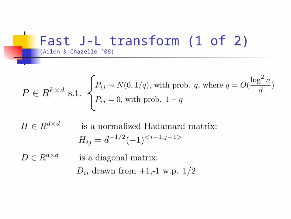
Fast J-L transform (1 of 2)(Ailon & Chazelle ’06)

Multiplication of the vectors by PHD is “fast”, since:
• (Du) is O(d) - since D is diagonal;• (HDu) is O(d logd) – use Fast Fourier Transform algorithms;• (PHDu) is O(poly (logn)) - P has on average O(poly(logn)) non-zeros per row.
Fast J-L transform (2 of 2)(Ailon & Chazelle ’06)

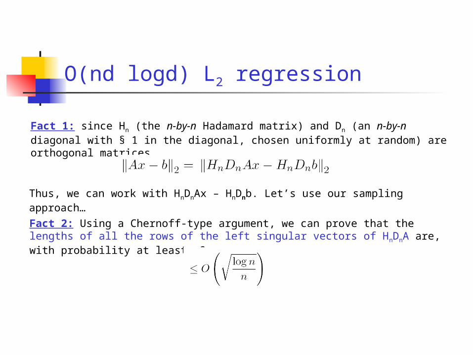
O(nd logd) L2 regression
Fact 1: since Hn (the n-by-n Hadamard matrix) and Dn (an n-by-n diagonal with § 1 in the diagonal, chosen uniformly at random) are orthogonal matrices,
Thus, we can work with HnDnAx – HnDnb. Let’s use our sampling approach…
O(nd logd) L2 regression
Fact 1: since Hn (the n-by-n Hadamard matrix) and Dn (an n-by-n diagonal with § 1 in the diagonal, chosen uniformly at random) are orthogonal matrices,
Fact 2: Using a Chernoff-type argument, we can prove that the lengths of all the rows of the left singular vectors of HnDnA are, with probability at least .9,
Thus, we can work with HnDnAx – HnDnb. Let’s use our sampling approach…

O(nd logd) L2 regression
DONE! We can perform uniform sampling in order to keep r = O(d logd/2) rows of HnDnA; our L2 regression theorem guarantees the accuracy of the approximation.
Running time is O(nd logd), since we can use the fast Hadamard-Walsh transform to multiply Hn and DnA.

Open problem: sparse approximations
Sparse approximations and l2 regression
(Natarajan ’95, Tropp ’04, ’06)
In the sparse approximation problem, we are given a d-by-n matrix A forming a redundant dictionary for Rd and a target vector b 2 Rd and we seek to solve
In words, we seek a sparse, bounded error representation of b in terms of the vectors in the dictionary.
subject to

Open problem: sparse approximations
Sparse approximations and l2 regression
(Natarajan ’95, Tropp ’04, ’06)
In the sparse approximation problem, we are given a d-by-n matrix A forming a redundant dictionary for Rd and a target vector b 2 Rd and we seek to solve
In words, we seek a sparse, bounded error representation of b in terms of the vectors in the dictionary.
This is (sort of) under-constrained least squares regression.
Can we use the aforementioned ideas to get better and/or faster approximation algorithms for the sparse approximation problem?
subject to
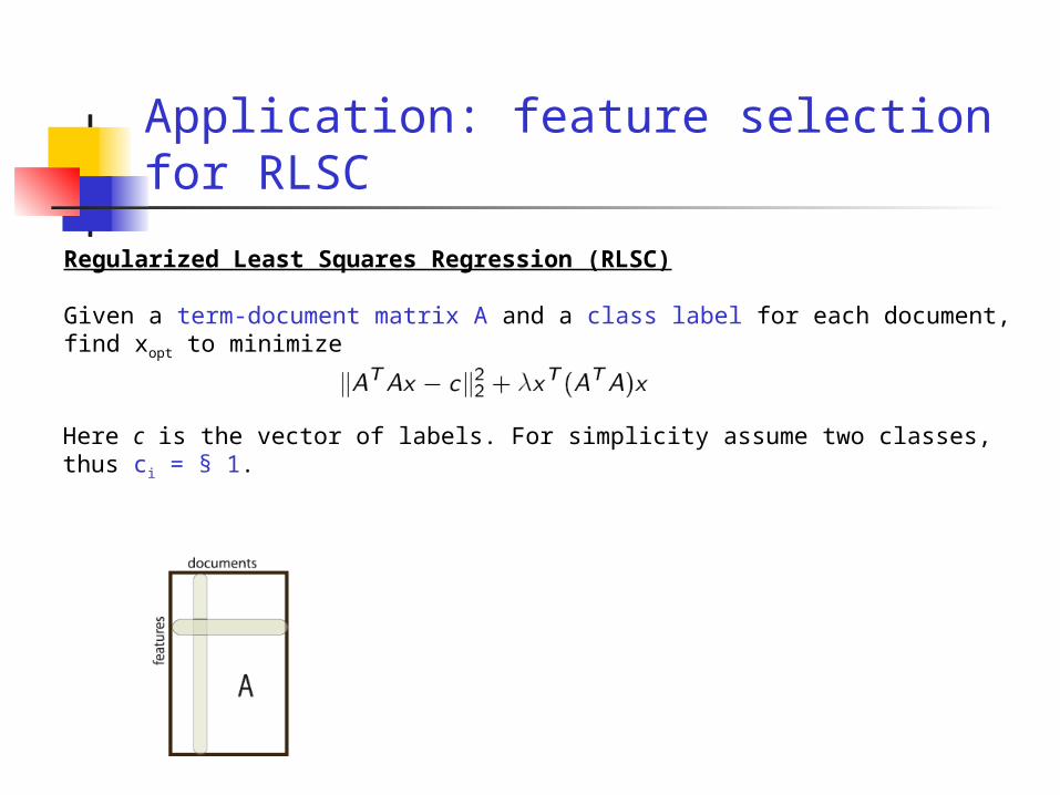
Application: feature selection for RLSC
Regularized Least Squares Regression (RLSC)
Given a term-document matrix A and a class label for each document, find xopt to minimize
Here c is the vector of labels. For simplicity assume two classes, thus ci = § 1.

Application: feature selection for RLSC
Regularized Least Squares Regression (RLSC)
Given a term-document matrix A and a class label for each document, find xopt to minimize
Here c is the vector of labels. For simplicity assume two classes, thus ci = § 1.Given a new document-vector q, its classification is determined by the sign of

Feature selection for RLSC
Feature selection for RLSC
Is it possible to select a small number of actual features (terms) and apply RLSC only on the selected terms without a huge loss in accuracy?
Well studied problem; supervised (they employ the class label vector c) algorithms exist.
We applied our L2 regression sampling scheme to select terms; unsupervised!

A smaller RLSC problem

A smaller RLSC problem

TechTC data from ODP(Gabrilovich and Markovitch ’04)
TechTC data
100 term-document matrices; average size ¼ 20,000 terms and ¼ 150 documents.
In prior work, feature selection was performed using a supervised metric called information gain (IG), an entropic measure of correlation with class labels.
Conclusion of the experiments
Our unsupervised technique had (on average) comparable performance to IG.


Conclusions
Linear Algebraic techniques (e.g., matrix decompositions and regression) are fundamental in data mining and information retrieval.
Randomized algorithms for linear algebra computations contribute novel results and ideas, both from a theoretical as well as an applied perspective.

Conclusions and future directions
Linear Algebraic techniques (e.g., matrix decompositions and regression) are fundamental in data mining and information retrieval.
Randomized algorithms for linear algebra computations contribute novel results and ideas, both from a theoretical as well as an applied perspective.
Important directions
• Faster algorithms
• More accurate algorithms
• Matching lower bounds
• Implementations and widely disseminated software
• Technology transfer to other scientific disciplines