randomized numerical linear algebra (randnla): past, present, and future, cont. to access our web...
TRANSCRIPT

Randomized Numerical Linear Algebra (RandNLA): Past, Present, and Future,
cont.
To access our web pages:
Petros DrineasPetros Drineas11 && Michael W. MahoneyMichael W. Mahoney22
1 1 Department of Computer Science, Rensselaer Polytechnic InstituteDepartment of Computer Science, Rensselaer Polytechnic Institute2 2 Department of Mathematics, Stanford UniversityDepartment of Mathematics, Stanford University
Drineas
Michael Mahoney
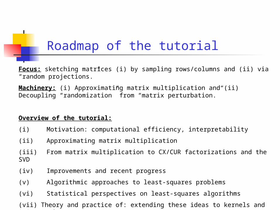
Focus: sketching matrices (i) by sampling rows/columns and (ii) via “random projections.”
Machinery: (i) Approximating matrix multiplication and (ii) Decoupling “randomization” from “matrix perturbation.”
Overview of the tutorial:
(i) Motivation: computational efficiency, interpretability
(ii) Approximating matrix multiplication
(iii) From matrix multiplication to CX/CUR factorizations and the SVD
(iv) Improvements and recent progress
(v) Algorithmic approaches to least-squares problems
(vi) Statistical perspectives on least-squares algorithms
(vii) Theory and practice of: extending these ideas to kernels and SPSD matrices
(viii) Theory and practice of: implementing these ideas in large-scale settings
Roadmap of the tutorial

Why randomized matrix algorithms?
• Faster algorithms: worst-case theory and/or numerical code
• Simpler algorithms: easier to analyze and reason about
• More-interpretable output: useful if analyst time is expensive
• Implicit regularization properties: and more robust output
• Exploit modern computer architectures: by reorganizing steps of alg
• Massive data: matrices that they can be stored only in slow secondary memory devices or even not at all
Already a big success … but why do they work?
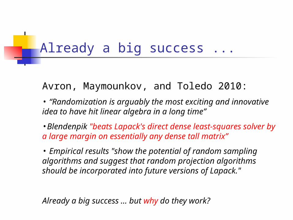
Already a big success ...
Avron, Maymounkov, and Toledo 2010:
• “Randomization is arguably the most exciting and innovative idea to have hit linear algebra in a long time”
•Blendenpik "beats Lapack's direct dense least-squares solver by a large margin on essentially any dense tall matrix”
• Empirical results "show the potential of random sampling algorithms and suggest that random projection algorithms should be incorporated into future versions of Lapack."Already a big success … but why do they work?

Already a big success ...
• Better worse-case theory: for L2 regression, L1 regression, low-rank matrix approximation, column subset selection, Nystrom approximation, etc.
• Implementations “beat” Lapack: for L2 regression on nearly any non-tiny tall dense matrix
• Low-rank implementations “better”: in terms of running time and/or robustness for dense/sparse scientific computing matrices
• Parallel and distributed implementations: exploit modern computer architectures to do computations on up to a tera-byte of data
• Genetics, astronomy, etc.: applications to choose good SNPs, wavelengths, etc. for genotype inference, galaxy identification, etc.
Already a big success … but why do they work?

A typical result: (1+ε)-CX/CUR
Theorem: Let TSVD,k time* be the time to compute an exact or approximate rank-k approximation to the SVD (e.g., with a random projection). Then, given an m-by-n matrix A, there exists** an algorithm that runs in O(TSVD,k) time that picks
at most roughly 3200*** (k/ε****) log (k/ε) columns of A
such that with probability at least 0.9*****
|| A – PCA||F ≤ (1+ε) || A – Ak ||F
*Isn’t that too expensive?
**What is it?
***Isn’t 3200 to big? Why do you need 3200?
****Isn’t 1/ε too bad for ε≅ 10 ?
*****Isn’t 0.1 too large a failure probability?

Why do these algorithms work?
They decouple randomness from vector space structure.
Today, explain this in the context of.• Least squares regression -> CX/CUR approximation
• CSSP -> Random Projections parameterized more flexibly
• Nystrom approximation of SPSD matrices
Permits finer control in applying the randomization.• Much better worst-case theory
• Easier to map to ML and statistical ideas
• Easier to parameterize problems in ways that are more natural to numerical analysts, scientific computers, and software developers
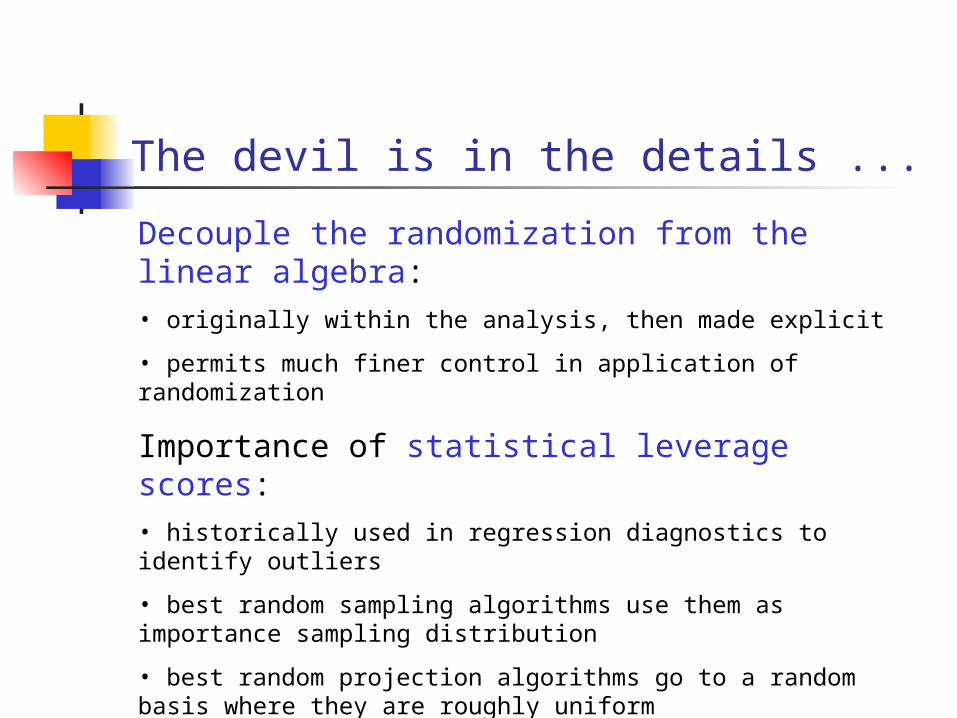
The devil is in the details ...
Decouple the randomization from the linear algebra:• originally within the analysis, then made explicit
• permits much finer control in application of randomization
Importance of statistical leverage scores:• historically used in regression diagnostics to identify outliers
• best random sampling algorithms use them as importance sampling distribution
• best random projection algorithms go to a random basis where they are roughly uniform
Couple with domain expertise—to get best results!

Statistical leverage, coherence, etc.
Definition: Given a “tall” n x d matrix A, i.e., with n > d, let U be any n x d orthogonal basis for span(A), & let the d-vector U(i) be the ith row of U. Then:
• the statistical leverage scores are i = ||U(i)||22 , for i {1,
…,n}
• the coherence is = maxi {1,…,n} i
• the (i,j)-cross-leverage scores are U(i)T U(j) = <U(i) ,U(j)>
Note: There are extension of this to:
• “fat” matrices A, with n, d are large and low-rank parameter k
• L1 and other p-norms
Mahoney and Drineas (2009, PNAS); Drineas, Magdon-Ismail, Mahoney, and Woodruff (2012, ICML)

History of Randomized Matrix Algs
How to “bridge the gap”?• decouple randomization from linear algebra
• importance of statistical leverage scores!
Theoretical origins
• theoretical computer science, convex analysis, etc.
• Johnson-Lindenstrauss
• Additive-error algs
• Good worst-case analysis
• No statistical analysis
Practical applications
• NLA, ML, statistics, data analysis, genetics, etc
• Fast JL transform
• Relative-error algs
• Numerically-stable algs
• Good statistical properties

Applications in: Astronomy
CMB Surveys (pixels) 1990 COBE
1000 2000 Boomerang
10,000 2002 CBI
50,000 2003 WMAP 1
Million 2008 Planck 10
Million
Galaxy Redshift Surveys (obj)• 1986 CfA 3500• 1996 LCRS 23000• 2003 2dF
250000• 2008 SDSS 1000000• 2012 BOSS
2000000• 2012 LAMOST 2500000
Angular Galaxy Surveys (obj)• 1970 Lick
1M• 1990 APM
2M• 2005 SDSS
200M• 2011 PS1
1000M• 2020 LSST
30000M
Time Domain• QUEST• SDSS Extension survey• Dark Energy Camera• Pan-STARRS• LSST…
“The Age of Surveys” – generate petabytes/year …
Szalay (2012, MMDS)

Galaxy properties from galaxy spectra
Continuum Emissions
Spectral Lines
Can we select “informative” frequencies (columns) or images (rows) “objectively”?
4K x 1M SVD Problem: ideal for randomized matrix algorithms
Szalay (2012, MMDS)

Galaxy diversity from PCA
[Average Spectrum]
[Stellar Continuum]
[Finer Continuum Features + Age]
[Age]Balmer series hydrogen lines
[Metallicity] Mg b, Na D, Ca II Triplet
1st
2nd
3rd
4th
5th
PC

Focus: sketching matrices by (i) sampling rows/columns and (ii) via “random projections.”
Machinery: (i) Approximating matrix multiplication and (ii) Decoupling “randomization” from “matrix perturbation.”
Overview of the tutorial:
(i) Motivation (computational efficiency, interpretability)
(ii) Approximating matrix multiplication
(iii) From matrix multiplication to CX/CUR factorizations and the SVD
(iv) Improvements and recent progress
(v) Algorithmic approaches to least-squares problems
(vi) Statistical perspectives on least-squares algorithms
(vii) Theory and practice of: extending these ideas to kernels and SPSD matrices
(viii) Theory and practice of: implementing these ideas in large-scale settings
Roadmap of the tutorial
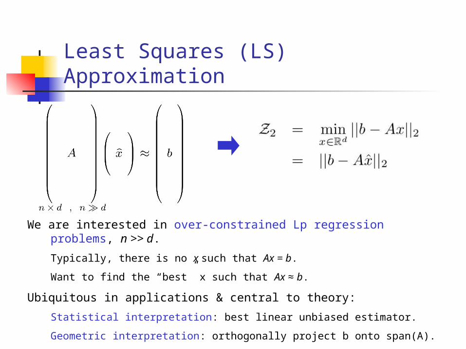
Least Squares (LS) Approximation
We are interested in over-constrained Lp regression problems, n >> d.
Typically, there is no x such that Ax = b.
Want to find the “best” x such that Ax ≈ b.
Ubiquitous in applications & central to theory:
Statistical interpretation: best linear unbiased estimator.
Geometric interpretation: orthogonally project b onto span(A).

Exact solution to LS Approximation
Cholesky Decomposition: If A is full rank and well-conditioned,
decompose ATA = RTR, where R is upper triangular, and
solve the normal equations: RTRx=ATb.
QR Decomposition: Slower but numerically stable, esp. if A is rank-deficient.
Write A=QR, and solve Rx = QTb.
Singular Value Decomposition:Most expensive, but best if A is very ill-conditioned.
Write A=UVT, in which case: xOPT = A+b = V-1kUTb.
Complexity is O(nd2) for all of these, but constant factors differ.
Projection of b on the subspace
spanned by the columns of A
Pseudoinverse of A

Modeling with Least Squares
Assumptions underlying its use:• Relationship between “outcomes” and “predictors is (roughly) linear.
• The error term has mean zero.
• The error term has constant variance.
• The errors are uncorrelated.
• The errors are normally distributed (or we have adequate sample size to rely on large sample theory).
Should always check to make sure these assumptions have not been (too) violated!

Statistical Issues and Regression Diagnostics
Model: b = Ax+ b = response; A(i) = carriers;
= error process s.t.: mean zero, const. varnce, (i.e., E(e)=0
and Var(e)=2I), uncorrelated, normally distributed
xopt = (ATA)-1ATb (what we computed before)
b’ = Hb H = A(ATA)-1AT = “hat” matrix
Hij - measures the leverage or influence exerted on b’i by bj,
regardless of the value of bj (since H depends only on A)
e’ = b-b’ = (I-H)b vector of residuals - note: E(e’)=0, Var(e’)=2(I-H)
Trace(H)=d Diagnostic Rule of Thumb: Investigate if Hii > 2d/n
H=UUT U is from SVD (A=UVT), or any orthogonal matrix for span(A)
Hii = |U(i)|22 leverage scores = row “lengths” of spanning orthogonal
matrix

A “classic” randomized algorithm (1of3)
Over-constrained least squares (n x d matrix A,n >>d)
• Solve:
• Solution:
Randomized Algorithm:
• For all i {1,...,n}, compute
• Randomly sample O(d log(d)/ ) rows/elements fro A/b, using {pi} as importance sampling probabilities.
• Solve the induced subproblem:
Drineas, Mahoney, and Muthukrishnan (2006, SODA & 2008, SIMAX)
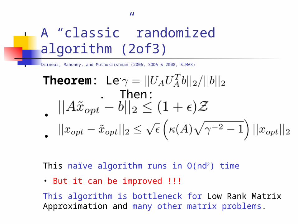
A “classic” randomized algorithm (2of3)
Theorem: Let . Then:
•
•
This naïve algorithm runs in O(nd2) time
• But it can be improved !!!
This algorithm is bottleneck for Low Rank Matrix Approximation and many other matrix problems.
Drineas, Mahoney, and Muthukrishnan (2006, SODA & 2008, SIMAX)

A “classic” randomized algorithm (3of3)
Sufficient condition for relative-error approximation.
For the “preprocessing” matrix X:
• Important: this condition decouples the randomness from the linear algebra.
• Random sampling algorithms with leverage score probabilities and random projections satisfy it!
Drineas, Mahoney, and Muthukrishnan (2006, SODA & 2008, SIMAX)
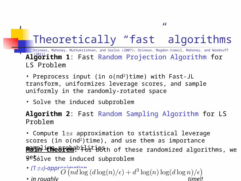
Theoretically “fast” algorithmsDrineas, Mahoney, Muthukrishnan, and Sarlos (2007); Drineas, Magdon-Ismail, Mahoney, and Woodruff (2011)
Main theorem: For both of these randomized algorithms, we get:
• (1)-approximation
• in roughly time!!
Algorithm 1: Fast Random Projection Algorithm for LS Problem
• Preprocess input (in o(nd2)time) with Fast-JL transform, uniformizes leverage scores, and sample uniformly in the randomly-rotated space
• Solve the induced subproblem
Algorithm 2: Fast Random Sampling Algorithm for LS Problem
• Compute 1 approximation to statistical leverage scores (in o(nd2)time), and use them as importance sampling probabilities
• Solve the induced subproblem
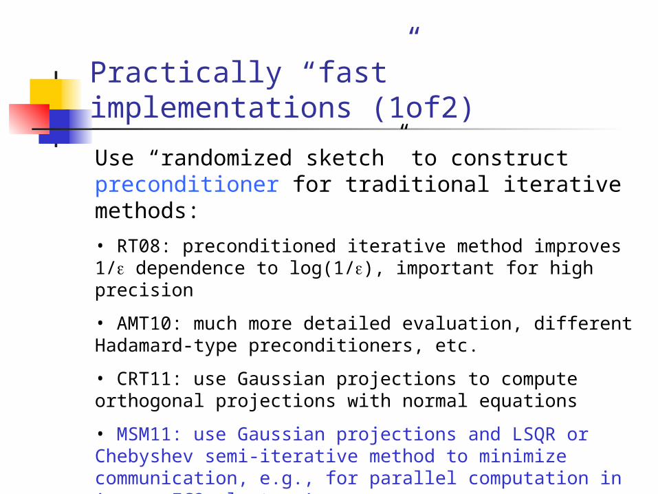
Practically “fast” implementations (1of2)
Use “randomized sketch” to construct preconditioner for traditional iterative methods:
• RT08: preconditioned iterative method improves 1/ dependence to log(1/), important for high precision
• AMT10: much more detailed evaluation, different Hadamard-type preconditioners, etc.
• CRT11: use Gaussian projections to compute orthogonal projections with normal equations
• MSM11: use Gaussian projections and LSQR or Chebyshev semi-iterative method to minimize communication, e.g., for parallel computation in Amazon EC2 clusters!

Practically “fast” implementations (2of2)
Avron, Maymounkov, and Toledo 2010:
• Blendenpik "beats Lapack's direct dense least-squares solver by a large margin on essentially any dense tall matrix”
• Empirical results "show the potential of random sampling algorithms and suggest that random projection algorithms should be incorporated into future versions of Lapack."

Ranking Astronomical Line Indices
(Worthey et al. 94; Trager et al. 98)
Subspace Analysis of Spectra Cutouts:
-Othogonality-Divergence-Commonality
(Yip et al. 2013 subm.)
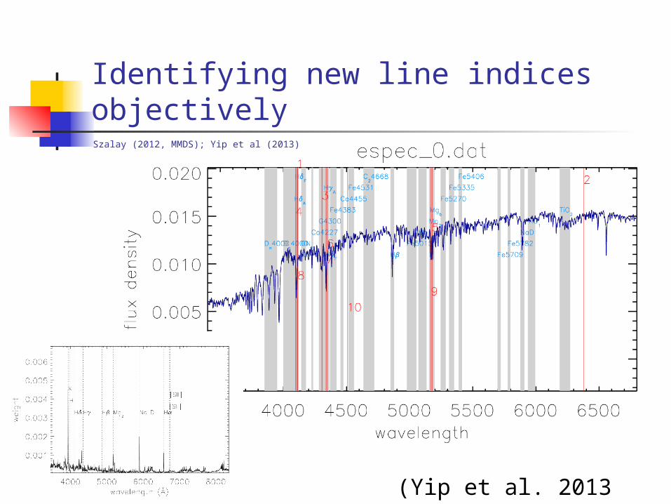
Identifying new line indices objectively
(Yip et al. 2013 subm.)
Szalay (2012, MMDS); Yip et al (2013)

New Spectral Regions (M2;k=5; overselecting 10X; combine if <30A)Szalay (2012, MMDS); Yip et al (2013)
Old Lick indices are “ad hoc”
New indices are “objective”
• Recover atomic lines
• Recover molecular bands
• Recover Lick indices
• Informative regions are orthogonal to each other, in contrast to Lick regions
(Yip et al. 2013 subm.)

Focus: sketching matrices by (i) sampling rows/columns and (ii) via “random projections.”
Machinery: (i) Approximating matrix multiplication and (ii) Decoupling “randomization” from “matrix perturbation.”
Overview of the tutorial:
(i) Motivation (computational efficiency, interpretability)
(ii) Approximating matrix multiplication
(iii) From matrix multiplication to CX/CUR factorizations and the SVD
(iv) Improvements and recent progress
(v) Algorithmic approaches to least-squares problems
(vi) Statistical perspectives on least-squares algorithms
(vii) Theory and practice of: extending these ideas to kernels and SPSD matrices
(viii) Theory and practice of: implementing these ideas in large-scale settings
Roadmap of the tutorial

A statistical perspective on “leveraging”
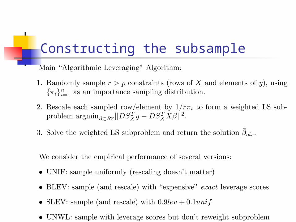
Constructing the subsample

Bias and variance of subsampling estimators (1 of 3)“A statistical perspective on algorithmic leveraging,” Ma, Mahoney, and Yu 2013
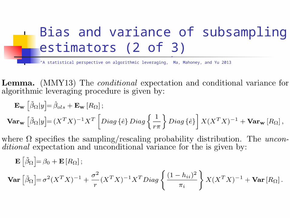
Bias and variance of subsampling estimators (2 of 3)“A statistical perspective on algorithmic leveraging,” Ma, Mahoney, and Yu 2013

Bias and variance of subsampling estimators (3 of 3)“A statistical perspective on algorithmic leveraging,” Ma, Mahoney, and Yu 2013
Consider empirical performance of several versions:
• UNIF: variance scales as n/r
• BLEV: variance scales as p/r but have 1/hii terms in denominator of sandwich expression
• SLEV: variance scales as p/r but 1/hii terms in denominator are moderated since no probabilities are too small
• UNWL: 1/hii terms are not in denominator, but estimates unbiased around βwls/β0
Estimates are unbiased (around βols/β0), but variance depends on sampling probabilities.
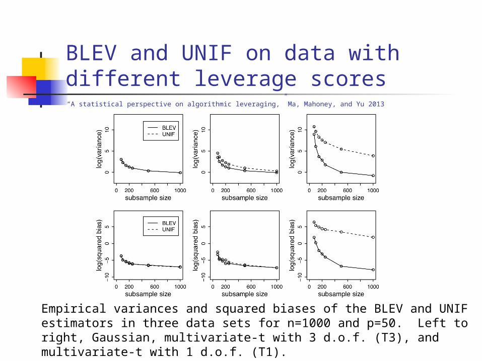
BLEV and UNIF on data with different leverage scores
Empirical variances and squared biases of the BLEV and UNIF estimators in three data sets for n=1000 and p=50. Left to right, Gaussian, multivariate-t with 3 d.o.f. (T3), and multivariate-t with 1 d.o.f. (T1).
“A statistical perspective on algorithmic leveraging,” Ma, Mahoney, and Yu 2013

BLEV and UNIF when rank is lost, 1
Comparison of BLEV and UNIF when rank is lost in the sampling process (n=1000 and p=10).
Left/middle/right panels: T3/T2/T1 data.
Upper panels: Proportion of singular X^TWX, out of 500 trials, for BLEV and UNIF .
Middle panels: Boxplots of ranks of 500 BLEV subsamples.
Lower panels: Boxplots of ranks of 500 UNIF subsamples.
Note the nonstandard scaling of the X axis.

BLEV and UNIF when rank is lost, 2
Comparison of BLEV and UNIF when rank is lost in the sampling process (n=1000 and p=10).
Left/middle/right panels: T3/T2/T1 data.
Upper panels: The logarithm of variances of the estimates.
Middle panels: The logarithm of variances, zoomed-in on the X-axis.
Lower panels: The logarithm of squared bias of the estimates.
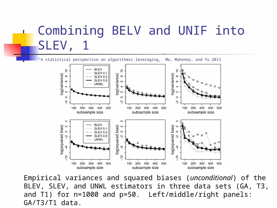
Combining BELV and UNIF into SLEV, 1
Empirical variances and squared biases (unconditional) of the BLEV, SLEV, and UNWL estimators in three data sets (GA, T3, and T1) for n=1000 and p=50. Left/middle/right panels: GA/T3/T1 data.
“A statistical perspective on algorithmic leveraging,” Ma, Mahoney, and Yu 2013
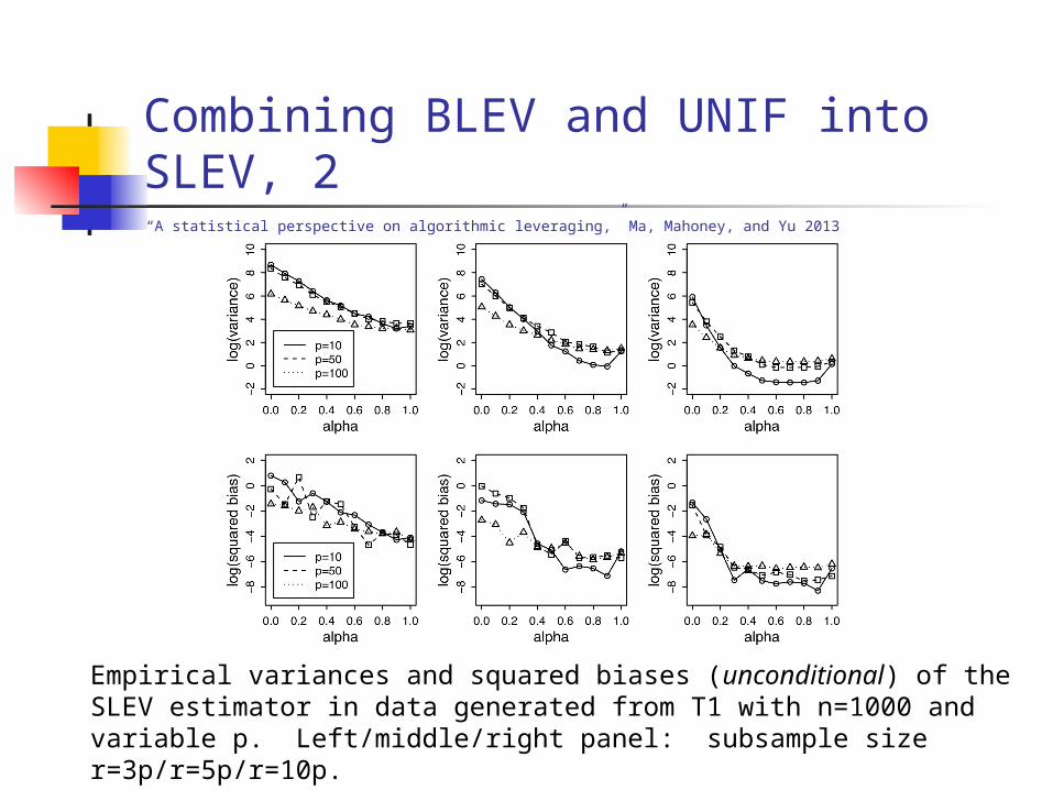
Combining BLEV and UNIF into SLEV, 2
Empirical variances and squared biases (unconditional) of the SLEV estimator in data generated from T1 with n=1000 and variable p. Left/middle/right panel: subsample size r=3p/r=5p/r=10p.
“A statistical perspective on algorithmic leveraging,” Ma, Mahoney, and Yu 2013

Results conditioned on the data
Empirical variances and squared biases (conditional) of the BLEV and UNIF estimators in 3 data sets (GA, T3, and T1) for n=1000 & p=50. Upper/lower panels: Variances/Squared bias. Left/middle/lower panels: GA/T3/T1 data.
“A statistical perspective on algorithmic leveraging,” Ma, Mahoney, and Yu 2013

Focus: sketching matrices by (i) sampling rows/columns and (ii) via “random projections.”
Machinery: (i) Approximating matrix multiplication and (ii) Decoupling “randomization” from “matrix perturbation.”
Overview of the tutorial:
(i) Motivation (computational efficiency, interpretability)
(ii) Approximating matrix multiplication
(iii) From matrix multiplication to CX/CUR factorizations and the SVD
(iv) Improvements and recent progress
(v) Algorithmic approaches to least-squares problems
(vi) Statistical perspectives on least-squares algorithms
(vii) Theory and practice of: extending these ideas to kernels and SPSD matrices
(viii) Theory and practice of: implementing these ideas in large-scale settings
Roadmap of the tutorial

41
Motivation (1 of 2)
Methods to extract linear structure from the data:
• Support Vector Machines (SVMs).
• Gaussian Processes (GPs).
• Singular Value Decomposition (SVD) and the related PCA.
Kernel-based learning methods to extract non-linear structure:
• Choose features to define a (dot product) space F.
• Map the data, X, to F by : XF.
• Do classification, regression, and clustering in F with linear methods.

42
Motivation (2 of 2)
• Use dot products for information about mutual positions.
• Define the kernel or Gram matrix: Gij=kij=((X(i)), (X(j))).
• Algorithms that are expressed in terms of dot products can be given the Gram matrix G instead of the data covariance matrix XTX.
If the Gram matrix G -- Gij=kij=((X(i)), (X(j))) -- is dense but (nearly) low-rank, then calculations of interest still need O(n2) space and O(n3) time:
• matrix inversion in GP prediction,
• quadratic programming problems in SVMs,
• computation of eigendecomposition of G.
Idea: use random sampling/projections to speed up these computations!
43
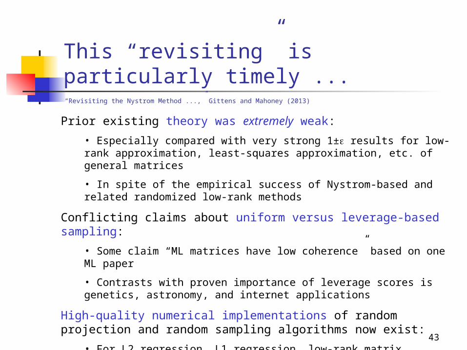
This “revisiting” is particularly timely ...
Prior existing theory was extremely weak:
• Especially compared with very strong 1± results for low-rank approximation, least-squares approximation, etc. of general matrices
• In spite of the empirical success of Nystrom-based and related randomized low-rank methods
Conflicting claims about uniform versus leverage-based sampling:
• Some claim “ML matrices have low coherence” based on one ML paper
• Contrasts with proven importance of leverage scores is genetics, astronomy, and internet applications
High-quality numerical implementations of random projection and random sampling algorithms now exist:
• For L2 regression, L1 regression, low-rank matrix approximation, etc. in RAM, parallel environments, distributed environments, etc.
“Revisiting the Nystrom Method ...,” Gittens and Mahoney (2013)

44
Some basics
Leverage scores:
• Diagonal elements of projection matrix onto the best rank-k space
• Key structural property needed to get 1± approximation of general matrices
Spectral, Frobenius, and Trace norms:
• Matrix norms that equal {∞,2,1}-norm on the vector of singular values
Basic SPSD Sketching Model:

45
Strategy for improved theory
Decouple the randomness from the vector space structure• This used previously with least-squares and low-rank CSSP approximation
This permits much finer control in the application of randomization• Much better worst-case theory
• Easier to map to ML and statistical ideas
• Has led to high-quality numerical implementations of LS and low-rank algorithms
• Much easier to parameterize problems in ways that are more natural to numerical analysts, scientific computers, and software developers
This implicitly looks at the “square root” of the SPSD matrix

46
Main structural resultGittens and Mahoney (2013)

47
Algorithmic applications (1 of 2)
Similar bounds for uniform sampling, except that need to sample proportional to the coherence (the largest leverage score).
Gittens and Mahoney (2013)

48
Algorithmic applications (2 of 2)
Similar bounds for Gaussian-based random projections.
Gittens and Mahoney (2013)

49
Data considered (1 of 2)

50
Data considered (2 of 2)

51
Weakness of previous theory (1 of 2)Drineas and Mahoney (COLT 2005, JMLR 2005):
• If sample (k -4 log(1/)) columns according to diagonal elements of A, then
Kumar, Mohri, and Talwalker (ICML 2009, JMLR 2012):
• If sample ( k log(k/)) columns uniformly, where ≈ coherence and A has exactly rank k, then can reconstruct A, i.e.,
Gittens (arXiv, 2011):
• If sample ( k log(k/)) columns uniformly, where = coherence, then
So weak that these results aren’t even a qualitative guide to practice

52
Weakness of previous theory (2 of 2)
53
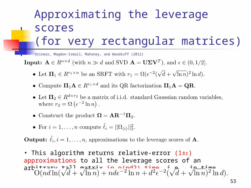
Approximating the leverage scores (for very rectangular matrices)
• This algorithm returns relative-error (1±) approximations to all the leverage scores of an arbitrary tall matrix in o(nd2) time, i.e., in time
Drineas, Magdon-Ismail, Mahoney, and Woodruff (2012)
54
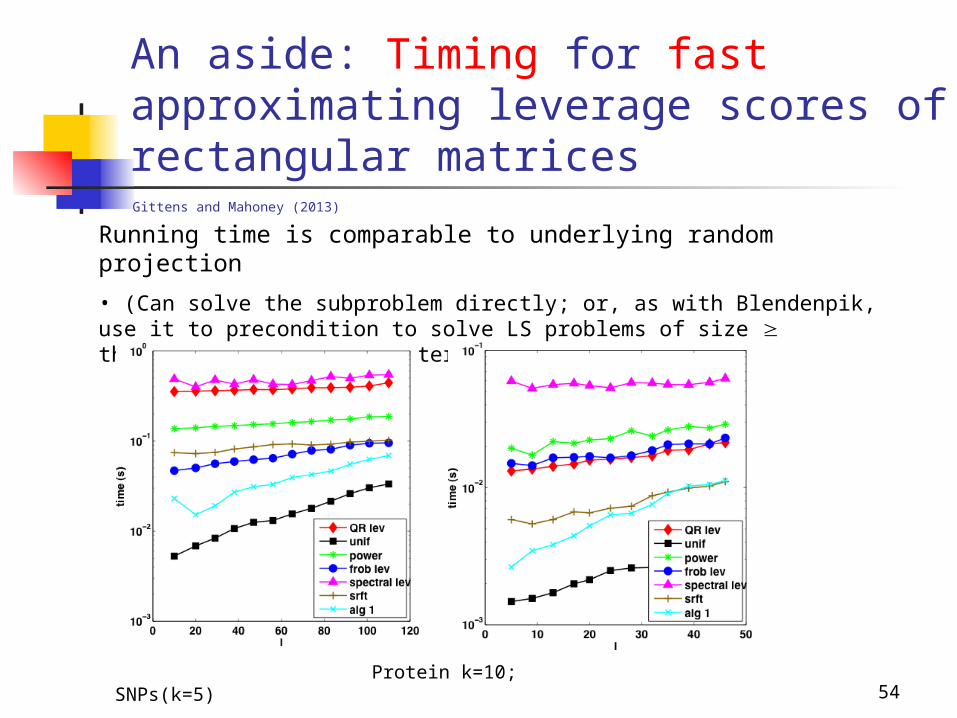
An aside: Timing for fast approximating leverage scores of rectangular matrices
Running time is comparable to underlying random projection
• (Can solve the subproblem directly; or, as with Blendenpik, use it to precondition to solve LS problems of size thousands-by-hundreds faster than LAPACK.)
Protein k=10; SNPs(k=5)
Gittens and Mahoney (2013)
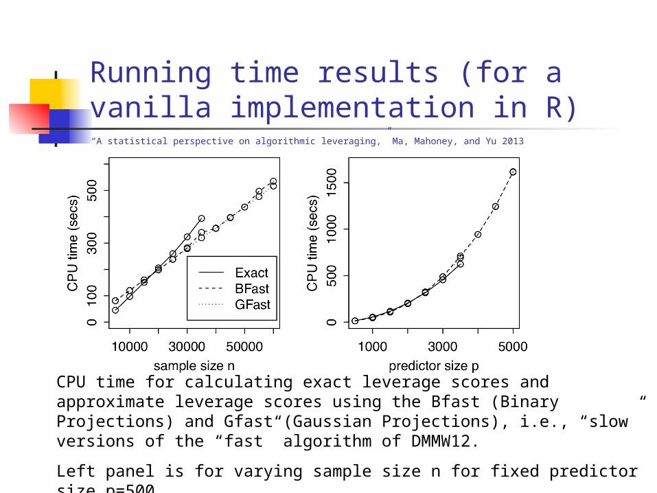
Running time results (for a vanilla implementation in R)“A statistical perspective on algorithmic leveraging,” Ma, Mahoney, and Yu 2013
CPU time for calculating exact leverage scores and approximate leverage scores using the Bfast (Binary Projections) and Gfast (Gaussian Projections), i.e., “slow” versions of the “fast” algorithm of DMMW12.
Left panel is for varying sample size n for fixed predictor size p=500.
Right panel is for varying predictor size p for fixed sample size n=20000.

56
Summary of running time issues
Running time of exact leverage scores: • worse than uniform sampling, SRFT-based, & Gaussian-based projections
Running time of approximate leverage scores: • can be much faster than exact computation• with q=0 iterations, time comparable to SRFT or Gaussian projection time• with q>0 iterations, time depends on details of stopping condition
The leverage scores: • with q=0 iterations, the actual leverage scores are poorly approximated• with q>0 iterations, the actual leverage scores are better approximated• reconstruction quality is often no worse, and is often better, when using approximate leverage scores
On “tall” matrices:• running time is comparable to underlying random projection• can use the coordinate-biased sketch thereby obtained as preconditioner for overconstrained L2 regression, as with Blendenpik or LSRN
Focus: sketching matrices by (i) sampling rows/columns and (ii) via “random projections.”
Machinery: (i) Approximating matrix multiplication and (ii) Decoupling “randomization” from “matrix perturbation.”
Overview of the tutorial:
(i) Motivation (computational efficiency, interpretability)
(ii) Approximating matrix multiplication
(iii) From matrix multiplication to CX/CUR factorizations and the SVD
(iv) Improvements and recent progress
(v) Algorithmic approaches to least-squares problems
(vi) Statistical perspectives on least-squares algorithms
(vii) Theory and practice of: extending these ideas to kernels and SPSD matrices
(viii) Theory and practice of: implementing these ideas in large-scale settings
Roadmap of the tutorial
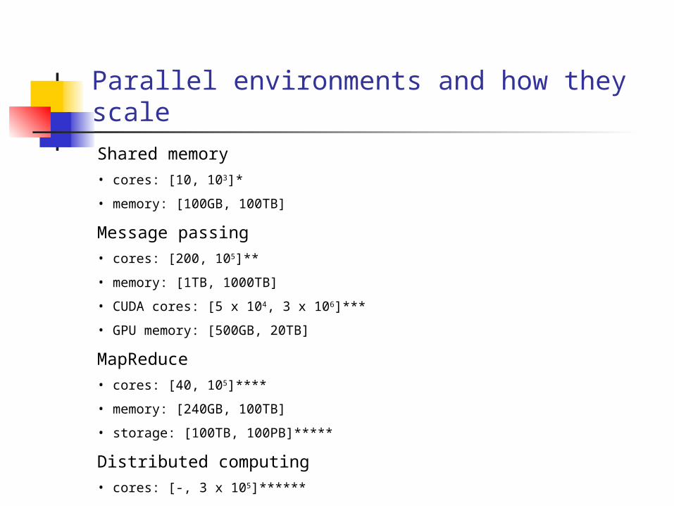
Parallel environments and how they scale
Shared memory• cores: [10, 103]*
• memory: [100GB, 100TB]
Message passing• cores: [200, 105]**
• memory: [1TB, 1000TB]
• CUDA cores: [5 x 10⁴, 3 x 10⁶]***
• GPU memory: [500GB, 20TB]
MapReduce• cores: [40, 105]****
• memory: [240GB, 100TB]
• storage: [100TB, 100PB]*****
Distributed computing• cores: [-, 3 x 10⁵]******

“Traditional” matrix algorithms
For L2 regression:• direct methods: QR, SVD, and normal equation (O(mn2 + n2) time)
• Pros: high precision & implemented in LAPACK• Cons: hard to take advantage of sparsity & hard to implement in parallel environments
• iterative methods: CGLS, LSQR, etc.• Pros: low cost per iteration, easy to implement in some parallel environments, & capable of computing approximate solutions• Cons: hard to predict the number of iterations needed
For L1 regression:• linear programming• interior-point methods (or simplex, ellipsoid? methods)• re-weighted least squares• first-order methods

Two important notions:leverage and conditionStatistical leverage. (Think: eigenvectors & low-precision solutions.)
• The statistical leverage scores of A (assume m>>n) are the diagonal elements of the projection matrix onto the column span of A.• They equal the L2-norm-squared of any orthogonal basis spanning A.• They measure:
• how well-correlated the singular vectors are with the canonical basis• which constraints have largest “influence" on the LS fit• a notion of “coherence” or “outlierness”
• Computing them exactly is as hard as solving the LS problem.
Condition number. (Think: eigenvalues & high-precision solutions.)
• The L2-norm condition number of A is (A) = σmax(A)/σmin(A).• κ(A) bounds the number of iterations
• for ill-conditioned problems (e.g., κ(A) ≅ 106 >> 1), convergence speed is slow.
• Computing κ(A) is generally as hard as solving the LS problem.
These are for the L2-norm. Generalizations exist for the L1-norm.

Meta-algorithm for L2 regression
1: Using the L2 statistical leverage scores of A, construct an importance sampling distribution {pi}i=1,...,m
2: Randomly sample a small number of constraints according to {pi}i,...,m to construct a subproblem.
3: Solve the L2-regression problem on the subproblem.
Naïve implementation: 1 + ε approximation in O(mn2/ε) time. (Ugh.)
“Fast” O(mn log(n)/ε) in RAM if
• Hadamard-based projection and sample uniformly
• Quickly compute approximate leverage scores
“High precision” O(mn log(n)log(1/ε)) in RAM if:
• use the random projection/sampling basis to construct a preconditioner
Question: can we extend these ideas to parallel-distributed environments?
(Drineas, Mahoney, etc., 2006, 2008, etc., starting with SODA 2006; Mahoney FnTML, 2011.)

Meta-algorithm for L1 (& Lp) regression
1: Using the L1 statistical leverage scores of A, construct an importance sampling distribution {pi}i=1,...,m
2: Randomly sample a small number of constraints according to {pi}i,...,m to construct a subproblem.
3: Solve the L1-regression problem on the subproblem.
Naïve implementation: 1 + ε approximation in O(mn5/ε) time. (Ugh.)
“Fast” in RAM if
• we perform a fast “L1 projection” to uniformize them approximately
• we approximate the L1 leverage scores quickly
“High precision” in RAM if:
• we use the random projection/sampling basis to construct an L1 preconditioner
Question: can we extend these ideas to parallel-distributed environments?
(Clakson 2005, DDHKM 2008, Sohler and Woodruff 2011, CDMMMW 2012, Meng and Mahoney 2012.)

LARGE versus large versus large:extending to parallel/distributed environments
Can we extend these ideas to parallel & distributed environments?
• Yes!!!
• Roughly, use the same meta-algorithm, but minimize communication rather than minimize flops
In the remainder, focus on L2 regression.
• Technical issues, especially for iterations, are very different for L2 regression versus L1/quantile regression
• Talk with me later if you care about L1 regression

LSRN: a fast parallel implementation
A parallel iterative solver based on normal random projections
• computes unique min-length solution to minx ||Ax-b||2
• very over-constrained or very under-constrained A
• full-rank or rank-deficient A
• A can be dense, sparse, or a linear operator
• easy to implement using threads or with MPI, and scales well in parallel environments
Meng, Saunders, and Mahoney (2011, arXiv)

LSRN: a fast parallel implementation
Algorithm:
• Generate a n x m matrix with i.i.d. Gaussian entries G
• Let N be R-1 or V -1 from QR or SVD of GA
• Use LSQR or Chebyshev Semi-Iterative (CSI) method to solve the preconditioned problem miny ||ANy-b||2
Things to note:
• Normal random projection: embarassingly parallel
• Bound (A): strong control on number of iterations
• CSI particularly good for parallel environments: doesn’t have vector inner products that need synchronization b/w nodes
Meng, Saunders, and Mahoney (2011, arXiv)
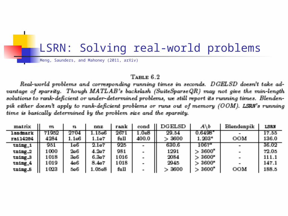
LSRN: Solving real-world problems
Meng, Saunders, and Mahoney (2011, arXiv)
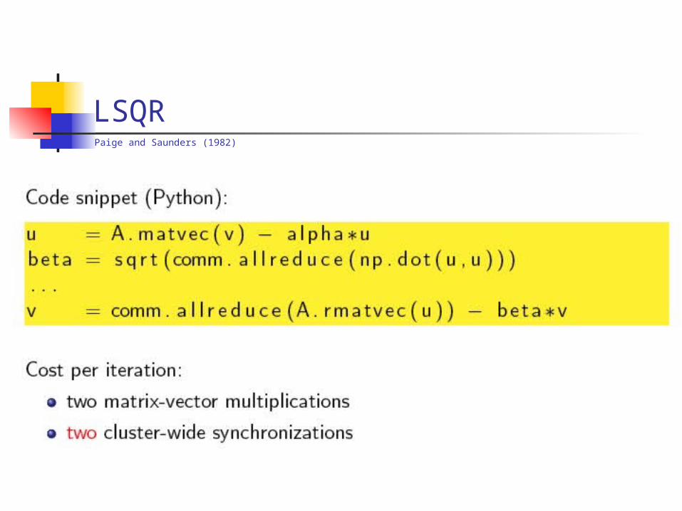
LSQRPaige and Saunders (1982)

Chebyshev semi-iterative (CSI)Golub and Varga (1961)
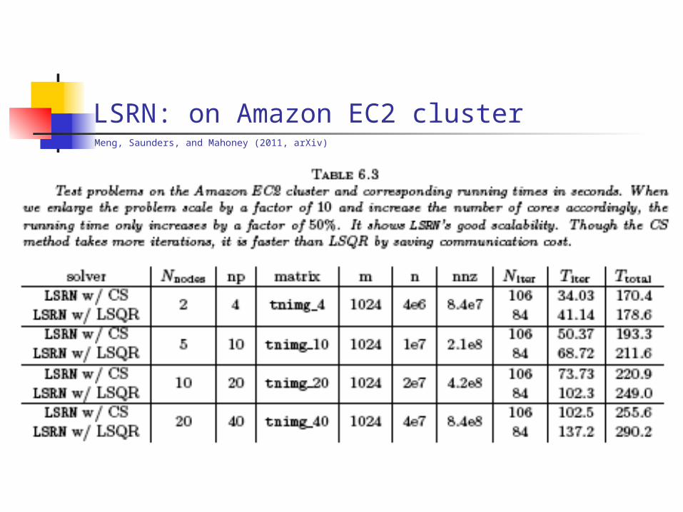
LSRN: on Amazon EC2 cluster
Meng, Saunders, and Mahoney (2011, arXiv)

Additional topics not covered ...
Theory/practice of L1/quantile regression:
• Cauchy transform, ellipsoidal rounding, etc. to get low-precision soln
• couple with randomized interior point cutting plane method to get moderate-precision solutions on a terabyte of data in Hadoop
Theory/practice of “input-sparsity” regression algorithms:
• input-sparsity time matrix multiplication result -> input-sparsity time L2 regression, low-rank approximation, leverage score algorithms
• nearly-input-sparsity time Lp regression algorithms via input-sparsity time low-distortion embeddings
Conclusions to Part IILeast-squares regression:
• faster sampling/projection in theory and implementation
• importance of decoupling randomness from vector space structure
Statistical perspective:
• better practical results without sacrificing worst-case quality
Revisiting the Nystrom method:
• the devil is in the details, if we want to make these algorithms useful in real large-scale systems
Implementing in parallel/distributed environments:
• the same meta-algorithms work, but highlights the limits of theoretically-useful models, and suggests future directions
All of these suggest future directions ...

Conclusions on “RandNLA”
Many many modern massive data sets are well-modeled by matrices:
• but existing algorithms were not designed for them
Randomization is a powerful tool for:
• the design of algorithms with better worst-case guarantees
• the design of algorithms with better statistical properties
• the design of algorithms for large-scale architectures
Great model/proof-of-principle for “bridging the gap”:
• between TCS and NLA and ML
• useful theory and theoretically-fruitful practice arises