Prepared by Dr. V. Valliammal

UNIT II-PART II

Random variable – Discrete Probability distribution –Continuous probability distributions – Expectation –Moment generating function – probability generating function - Probability mass and density functions.

1

Random VariablesRandom variableA real variable (X) whose value is determined by theoutcome of a random experiment is called arandom variable.(e.g) A random experiment consists of two tossesof a coin. Consider the random experiment which isthe number of heads (0, 1 or2)Outcome: HH HT TH TTValue of X: 2 1 1 0

2

Discrete Random Variable

A random variable x which takes a countable number of real values is called a discrete random variable.

(e.g) 1. number of telephone calls per unit time2. marks obtained in a test3. number of printing mistakes in each

page of a book

3

Probability Mass FunctionIf X is a discrete random variable taking atmost acountably infinite number of values x1, x2, .., weassociate a number Pi = P(X = xi) = P(xi), called theprobability mass function of X. The function P(xi)satisfies the following conditions:(i) P(xi) 0 i = 1, 2, …,

(ii) 1)P(x1i

i

4

Continuous Random Variable

A random variable X is said to be continuous if it can take all possible values between certain limits.

(e.g.)1. The length of a time during which a vacuum tube installed is a continuous random variable .

2. number of scratches on a surface, proportion of defective parts among 1000 tested,3. number of transmitted in error.

5

Probability Density FunctionConsider a small interval (x, x+dx) of length dx.The function f(x)dx represents the probability thatX falls in the interval (x, x+dx)i.e., P(x X x+dx) = f(x) dx.The probability function of a continuous randomvariable X is called as probability density functionand it satisfies the following conditions.(i) f(x) 0 x

(ii) 1f(x)dx

6

Distribution FunctionThe distribution function of a random variable X isdenoted as F(X) and is defined as F(x) = P(X x).The function is also called as the cumulativeprobability function.

when X is discrete

when X is continuous

x

xP(x)x)P(XF(x)

x

F(x)dx

7

Properties on Cumulative Distribution

1. If x b, F(a) F(b), where a and b are realquantities.

2. If F is the distribution function of a one-dimensional random variable X, then 0 F(x) 1.

3. If F is the distribution function of a onedimensional random variable X, then F() = 0 andF() = 1.

8

Problems1. If a random variable X takes the values 1, 2, 3, 4such that 2P(X=1)=3P(X=2)=P(X=3)=5P(X=4). Findthe probability distribution of X.Solution:Assume P(X=3) = α By the given equation

For a probability distribution (and mass function) P(x) = 1P(1)+P(2)+P(3)+P(4) =1

5α4)P(X

3α2)P(X

2α1)P(X

9

The probability distribution is given by

61301

30611

532

616)4(;

6130)3(;

6110)2(;

6115)1( XPXPXPXP

616

6130

6110

6115)(

4321

xp

X

10

2. Let X be a continuous random variable having the probability density function

Find the distribution function of x.Solution:

otherwise

xxxf,0

1,2)( 3

21

21

31

1112)()(xx

dxx

dxxfxFxxx

11

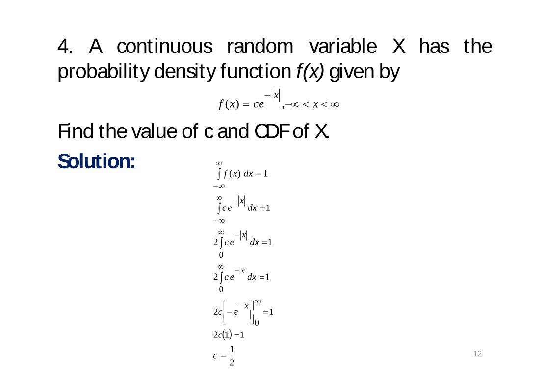
4. A continuous random variable X has theprobability density function f(x) given by

Find the value of c and CDF of X.Solution:

xcexfx

,)(

21

112

12

12

12

1

1)(

0

0

0

c

c

ec

dxec

dxec

dxec

dxxf

x

x

x

x

12

x

xx

x x

xx

x

e

ec

dxec

dxec

dxxfxF

xiCase

21

)(

0)(

x

x

x

xxx

x xx

xx

x

e

ec

ccec

ecec

dxecdxec

dxec

dxxfxF

xiiCase

221

2

)(

0)(

0

00

0

0,221

0,21

)(xe

xexF x

x

13

5. A random variable X has the followingprobability distribution.X: 0 1 2 3 4 5 6 7f(x): 0 k 2k 2k 3k k2 2k2 7k2+kFind (i) the value of k (ii) p(1.5 < X < 4.5 | X >2) and(iii) the smallest value of λ such that p(X≤λ) > 1/2.Solution(i)

1.0101

101,101910

1k 7k2kk3k2k2kk0

1)(

2

222

k

kkk

xP

14

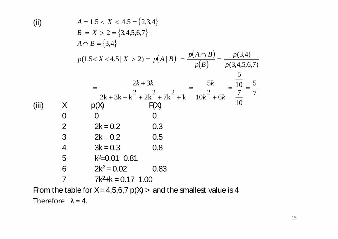
(ii)

(iii) X p(X) F(X)0 0 02 2k = 0.2 0.33 2k = 0.2 0.54 3k = 0.3 0.85 k2=0.01 0.816 2k2 = 0.02 0.837 7k2+k = 0.17 1.00

From the table for X = 4,5,6,7 p(X) > and the smallest value is 4Therefore λ = 4.

)7,6,5,4,3(

)4,3(|)2|5.45.1(

4,37,6,5,4,32

4,3,25.45.1

pp

BpBApBApXXp

BAXB

XA

75

107

105

610

5

k 7k2kk3k2k

322222

kk

kkk

15

Expectation of a Random VariableThe expectation of a random variable X is denotedas E(X). It returns a representative value for aprobability distribution.For a discrete probability distribution

E(X) = x p(x).For a continuous random variable X which

assumes values in (a, b)

b

a

xf(x)dxE(X)

16

Properties on Expectation1. Expectation of a constant is a constant.2. E[aX] = aE(X), where a is a constant.3. E(aX + b) = aE(X) + b, where a and b are

constants.4. |E(X)| E|X|, for any random variable X.5. If X Y, E(X) E(Y).

17

Variance of a Random VariableThe variance of a Random variable X, which isrepresented as V(X) is defined as the expectationof squares of the derivations from the expectedvalue.

V(X) = E(X2) – (E(X))2

Properties On Variance1. Variance of a constant is 0.2. V(aX) = a V(X), where a is a constant.

18

Moments and Other Statistical ConstantsRaw MomentsRaw moments about origin

Raw moments about any arbitrary value A

Central moments

b

a

rr f(x)dxxμ

b

a

rr f(x)dxA)(xμ

b

a

rrr f(x)dxE(X))(XE(X)]E[Xμ

19

Relationship between Raw Moments and CentralMoments

(always)0μ1

2122 μμμ

311233 μ2μμ3μμ

41

2121344 μ3μμ6μμ4μμ

20

Moment Generating Function (M.G.F)

It is a function which automatically generates theraw moments. For a random variable X, themoment generating function is denoted as MX(t)and is derived as MX(t) = E(etX).Reason for the name M.G.F

3!Xt

2!XttX1E

2322

2!XtEE(tx)E(1)

22

)()( txX eEtM

21

Here = coefficient of t in MX(t)

= coefficient of in MX(t)

In general = coefficient of in MX(t).

1μ

2μ2!t 2

rμ 2!t 2

)E(X2!ttE(X)1 2

2

2

2

1 μ2!tμt1

22

Problems1. The p.m.f of a RV X, is given by Find MGF, meanand variance.Solution

....2222

2

21

)(

432

0

0

tttt

x

xt

xx

tx

txtXX

eeee

e

e

xpeeEtM

t

t

t

t

ttttt

ee

ee

eeeee

22

1

12

..2222

12

432

23

Differentiating twice with respect to t

put t = 0 above

222

2

2

2

t

t

t

tttt

Xe

e

e

eeeetM

3

2

4

2

2

24

2

22222

t

tt

t

ttttt

X

e

ee

e

eeeeetM

20)( XMXE

246

6022

2

XEXEVariance

MXE X

24

2. Find MGF of the RV X, whose pdf is given by andhence find the first four central moments.Solution

t

te

dxe

dxee

dxxfeeEtM

xt

xt

xtx

txtXX

0

0

0

25

Expanding in powers of t

Taking the coefficient we get the raw momentsabout origin

...11

1 32

ttt

tttM X

222 2!2

1!1

toftcoefficienXE

toftcoefficienXE

4

44

333

24!4

6!3

toftcoefficienXE

toftcoefficienXE

26

and the central moments are

4442234

41

413

212213144

33223

31

211212133

2222

2111122

1

911412616424444

21113123633

111222

0

CCC

CC

C

27

3. If the MGF of a (discrete) RV X is find thedistribution of X and p ( X = 5 or 6).Solution

By definition

te45

1

...5

45

45

4151

5415

1451

32 ttt

ttX

eee

eetM

...)2()1()0(1

)(

20

pepepe

xpeeEtM

ttt

txtXX

28