1

Continuous random variables

f(x)

x

2

Continuous random variables

A discrete random variable has values that are isolated numbers, e.g.:

Number of boys in a family

number of heads in 10 flips of a coin

A continuous random variable has values over an entire interval, e.g.:

Height of people

All values in the interval [2.2,8.2]

3

Difference between discrete and continuous rv’s

In the random numbers table, every digit 0,1,…,9 has the same probability of 0.1 to be selected.

S={0,1,2,3,4,5,6,7,8,9}

Probability histogram:

0 1 2 3 4 5 6 7 8 9

4

Difference between discrete and continuous rv’s

Now suppose that we want to choose at random a number in [0,1].You can visualize such a random number by thinking of a spinner that turns freely on its axis and slowly comes to stop:

½

¼

0

¾

In this case, the sample space is an interval:

S={all numbers x such that 0≤x≤1}

5

Difference between discrete and continuous rv’s

S={all numbers x such that 0≤x≤1}

We want all possible outcomes to be equally likely.

However

Impossible to assign a probability to each x because there are infinitely many x’s.

½

¼

0

¾

6

Difference between discrete and continuous rv’s

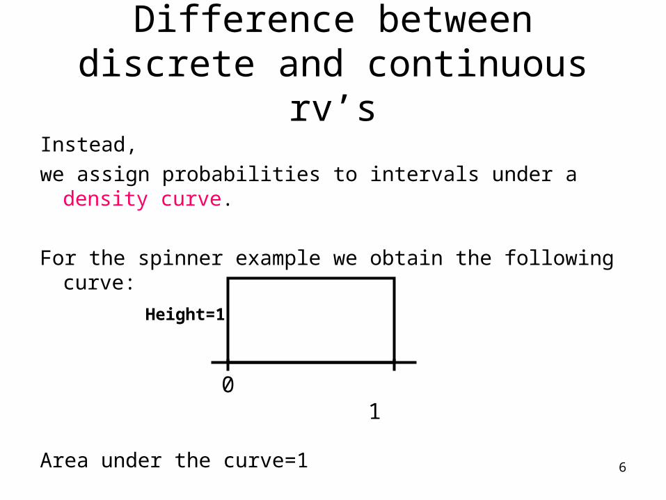
Instead,

we assign probabilities to intervals under a density curve.

For the spinner example we obtain the following curve:

Area under the curve=1

0 1

Height=1

7

Difference between discrete and continuous rv’s

What is the probability of a number between 0.2 and 0.6?

0 .2 .6 1

Area = (.6-.2)1=0.4

=p(.2≤x≤.6)

p(X≥7)=

Height=1

.3

8

Continuous random variable

1. Takes all values in an interval

2. The probability distribution is described by a density curve f(x)

3. f(x)≥0 for all x

4. The probability of any event is the area under the density curve and above the values of X that make up the event

9

Continuous random variable

5. All continuous distributions assign probability zero to every individual outcome

0 .2 1

P(X=.2)=0

Since P(X=.2)=0 P(X>.2)=p(X≥.2)

(this is true only for continuous rv’s)

10

Only intervals of values have positive probability:

0 1.79 .81

P(.79≤X≤.81)=0.02

0 1.799 .801

.7999 .8001

P(.799≤X≤.801)=0.002

P(.7999≤X≤.8001)=0.0002

11

An interval of size zero has a probability of zero:

0 1 .80

P(.8≤X≤.8)=

P(X=8)=0

12

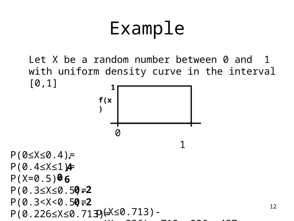
Example

Let X be a random number between 0 and 1 with uniform density curve in the interval [0,1]

0 1

f(x)

1

P(0≤X≤0.4)=P(0.4≤X≤1)=P(X=0.5)=P(0.3≤X≤0.5)=P(0.3<X<0.5)=P(0.226≤X≤0.713)=

.4.6

00.20.2

p(X≤0.713)-p(X≤.226)=.713-.226=.487

13

Example

A random number generator produces numbers from 1 to 3 with a uniform density curve as follows.

1 3

f(x)

1. What is the height of the density curve?

Since the area under the curve is 1, the height must be ½

2. P(1≤X≤3)= P(2≤X≤3)= P(1≤X≤1.8)= P(1.8<X≤2.5)=

1p(X≤3)-p(X≤2)=1-0.5

p(X≤1.8)-p(X≤1)=(0.8)(½)-0=.4p(X≤2.5)-p(X<1.8)=(2.5-1)(½)-(1.8-1)(½)=.75-.4=.35

14

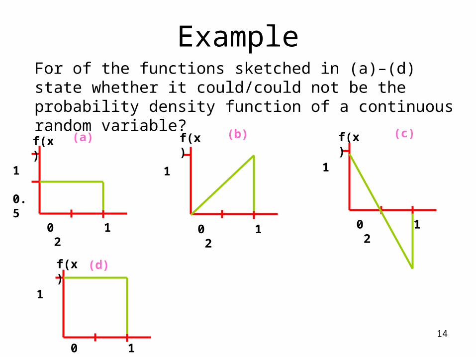
ExampleFor of the functions sketched in (a)–(d) state whether it could/could not be the probability density function of a continuous random variable?

0 1 2

1

0.5

0 1 2

1 1

0 1 2

1

0 1 2

(a) (b) (c)

(d)

f(x) f(x) f(x)

f(x)

15

Example

For the following probability density function, which of the two intervals is assigned a higher probability:

P(0<X<.5) Or P(1.5<X<2) ?

1

0 1 2

f(x)

16

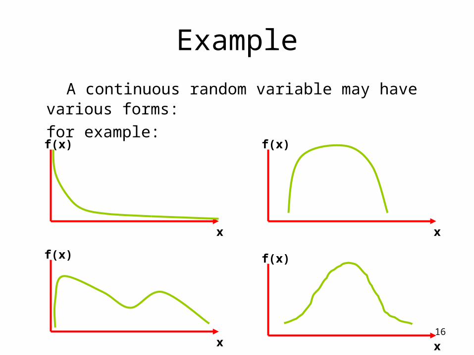
Example

A continuous random variable may have various forms:

for example:

f(x)

x

f(x)

x

f(x)

x

f(x)

x

17

Normal distribution as a continuous distribution

N(μ,σ) is a normal distribution with mean μ and standard deviation σ

If X~N(μ,σ), then

μ

Density curve

N(0,1)~σ

μXZ

18

Normal distribution as a continuous distribution

ExampleScores in a certain exam are distributed normally with Mean 80 and SD 12.

1. What proportion of students receive a score higher than 86?

P(X>86)=

= p(Z>.5) = 1-Ф(.5) = 1-.6915=.3085

30.85% of the students received a score higher than 86

12

8086

12

80Xp

19

2. What is the probability to receive a score that differs from the mean by no more than 10 points?

p(70≤X≤90)=

=

=p(-.833≤Z≤.833)= Ф(.8333)- Ф(-.8333)=.7967-.2033=.5936

8070 90

12

8090

12

80X

12

8070p

20

3. Find the third quarter of the scores (find Q3)

We first find Q3 on the z-scale and then convert it to x-scale.

z0.75=0.675 ( p(Z≤.675)=0.75 )

Q3 = 0.675(12)+80 = 88.1

12

80675.0 3

Q

80 Q3

21

4. The lowest 5% of the scores are below which score?

We first find x on the z-scale and then convert it to x-scale.

z0.05=-1.645 ( p(Z≤-1.645)=0.05 )

x=-1.6-1.645(12)+80 = 60.26

x 80

5%

12

801.645-

x