Lesson 99 -

Continuous Random

Variables

HL Math - Santowski

Consider the following table of heights of palm

trees, measured in mm, divided into intervals of

1000’s of mm,

interval Frequency

(0,1000] 0

(1000,2000] 50

(2000,3000] 250

(3000,4000] 300

(4000,5000] 250

(5000,6000] 100

(6000,7000] 50

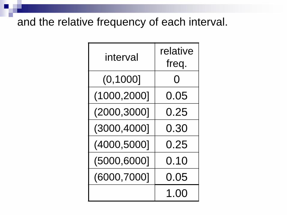
and the relative frequency of each interval.

intervalrelative

freq.

(0,1000] 0

(1000,2000] 0.05

(2000,3000] 0.25

(3000,4000] 0.30

(4000,5000] 0.25

(5000,6000] 0.10

(6000,7000] 0.05

1.00

Graph

interval relative freq.

(0,1000] 0

(1000,2000] 0.05

(2000,3000] 0.25

(3000,4000] 0.30

(4000,5000] 0.25

(5000,6000] 0.10

(6000,7000] 0.05

0 1000 2000 3000 4000 5000 6000 7000

sales

f(x) = p(x)

0

The area of each bar is the frequency of the category.

Tree height

Graph

interval relative freq.

(0,1000] 0

(1000,2000] 0.05

(2000,3000] 0.25

(3000,4000] 0.30

(4000,5000] 0.25

(5000,6000] 0.10

(6000,7000] 0.05

0 1000 2000 3000 4000 5000 6000 7000

sales

f(x) = p(x)

0

Here is the frequency polygon.

Tree height

If we make the intervals 500 mm instead of 1000

mm, the graph would probably look something like

this:

tree height

f(x) = p(x)

The height of the

bars increases and

decreases more

gradually.

If we made the intervals infinitesimally small, the

bars and the frequency polygon would become

smooth, looking something like this:

f(x) = p(x)

Tree height

This what the distribution

of a continuous random

variable looks like.

This curve is denoted f(x)

or p(x) and is called the

probability density

function.

pmf versus pdf

For a discrete random variable, we had a probability mass function (pmf).

The pmf looked like a bunch of spikes, and probabilities were represented by the heights of the spikes.

For a continuous random variable, we have a probability density function (pdf).

The pdf looks like a curve.

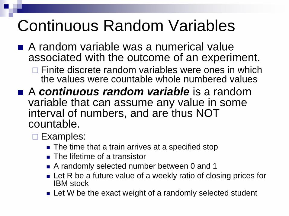
Continuous Random Variables

A random variable was a numerical value associated with the outcome of an experiment. Finite discrete random variables were ones in which

the values were countable whole numbered values

A continuous random variable is a random variable that can assume any value in some interval of numbers, and are thus NOT countable. Examples:

The time that a train arrives at a specified stop

The lifetime of a transistor

A randomly selected number between 0 and 1

Let R be a future value of a weekly ratio of closing prices for IBM stock

Let W be the exact weight of a randomly selected student

1. They are used to describe different types of quantities.

2. We use distinct values for discrete random variables

but continuous real numbers for continuous random

variables.

3. Numbers between the values of discrete random

variable makes no sense, for example, P(0)=0.5, P(1)=0.5,

then P(1.5) has no meaning at all. But that is not true for

continuous random variables.

Difference between discrete and

continuous random variables

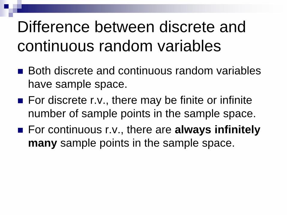
Both discrete and continuous random variables

have sample space.

For discrete r.v., there may be finite or infinite

number of sample points in the sample space.

For continuous r.v., there are always infinitely

many sample points in the sample space.

Difference between discrete and

continuous random variables

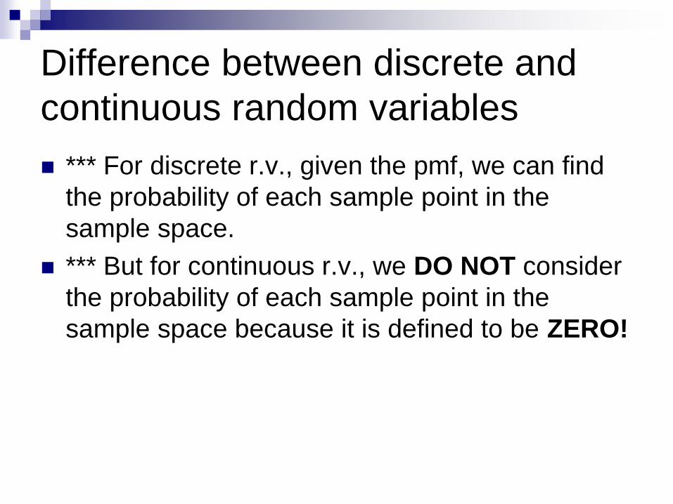
*** For discrete r.v., given the pmf, we can find

the probability of each sample point in the

sample space.

*** But for continuous r.v., we DO NOT consider

the probability of each sample point in the

sample space because it is defined to be ZERO!

Difference between discrete and

continuous random variables

Continuous Random Variables A random variable is said to be continuous if there is a function fX(x)

with the following properties: Domain: all real numbers

Range: fX(x)≥0

The area under the entire curve is 1

Such a function fX(x) is called the probability density function(abbreviated p.d.f.)

The fact that the total area under the curve fX(x) is 1 for all X values of the random variable tells us that all probabilities are expressed in terms of the area under the curve of this function. Example: If X are values on the interval from [a,b], then the P(a≤X≤b) =

area under the graph of fX(x) over the interval [a,b]

A

a b

fX

Continuous Random Variables

Because all probabilities for a continuous

random variable are described in terms of the

area under the p.d.f. function, the P(X=x) = 0.

Why: the area of the p.d.f. for a single value is zero

because the width of the interval is zero!

That is, for any continuous random variable, X,

P(X = a) = 0 for every number a. This DOES NOT

imply that X cannot take on the value a, it simply

means that the probability of that event is 0.

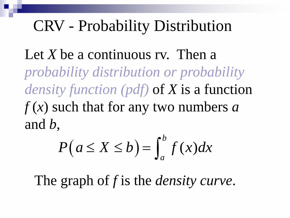
CRV - Probability Distribution

Let X be a continuous rv. Then a

probability distribution or probability

density function (pdf) of X is a function

f (x) such that for any two numbers a

and b,

( )b

aP a X b f x dx

The graph of f is the density curve.

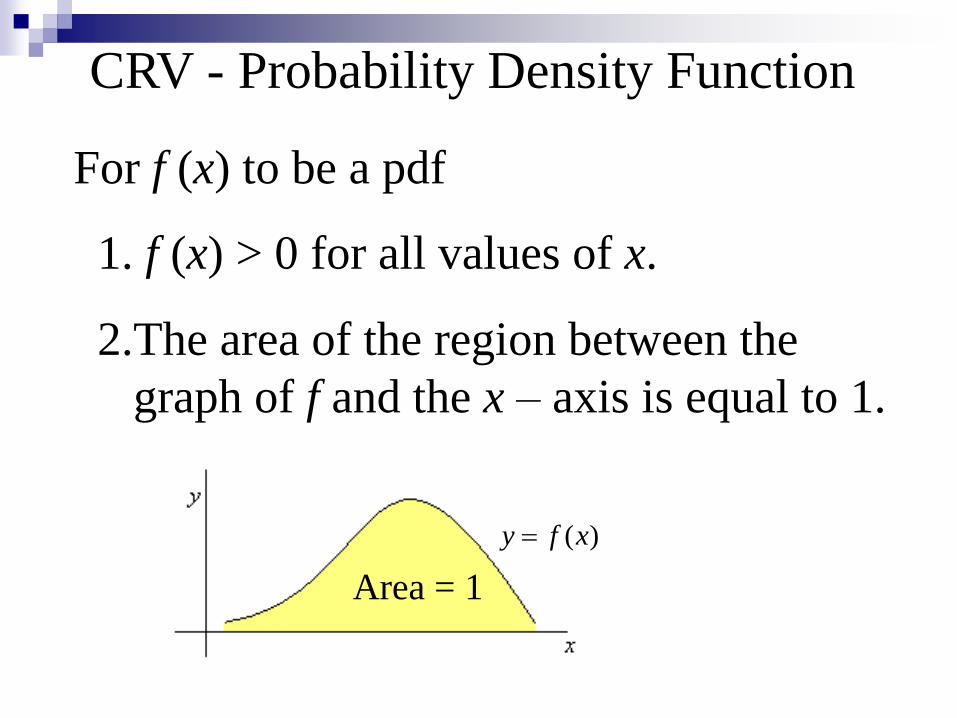
CRV - Probability Density Function

For f (x) to be a pdf

1. f (x) > 0 for all values of x.

2.The area of the region between the

graph of f and the x – axis is equal to 1.

Area = 1

( )y f x

CRV - Probability Density Function

is given by the area of the shaded

region.

( )y f x

ba

( )P a X b

Example

The p.d.f. of T, the weekly CPU time (in

hours) used by an accounting firm, is

given below.

4 if1

40 if)4(

0 if0

)( 2

64

3

t

ttt

t

tfT

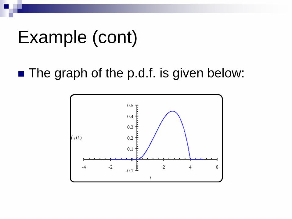
Example (cont)

The graph of the p.d.f. is given below:

-0.1

0

0.1

0.2

0.3

0.4

0.5

-4 -2 0 2 4 6

t

f T (t )

Example (cont)

is equal to the area between the

graph of and the t-axis over the interval.

)21( TP

-0.1

0

0.1

0.2

0.3

0.4

0.5

-4 -2 0 2 4 6

t

f T (t )

Example

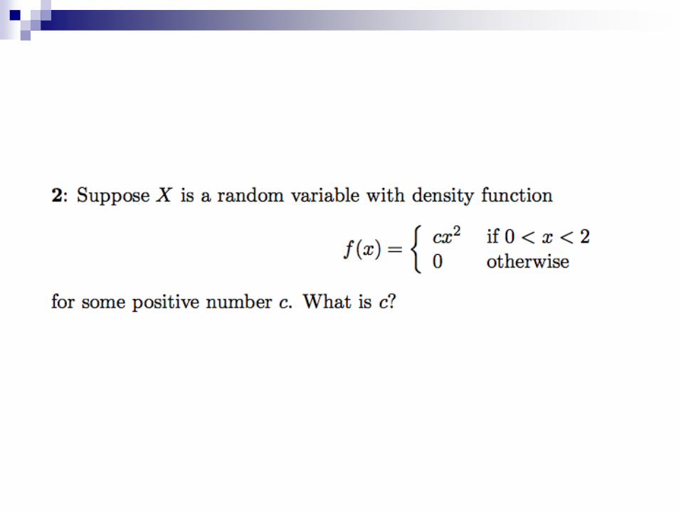
Sketch the following functions and decide whether they are valid pdfs

2 0 5

0 otherwise

x xf x

–1 1 2 3 4 5 6

–4

–3

–2

–1

1

2

3

4

x

y

13

0 3

0 otherwise

x xf x

–1 1 2 3 4

–1

–0.5

0.5

1

1.5

2

x

y

Sketch the following function and decide whether it is a valid pdf

23

2 -1 1

0 otherwise

x xf x

–2 –1 1 2

–2

–1

1

2

x

y

Sketch the following function and decide whether it is a valid pdf

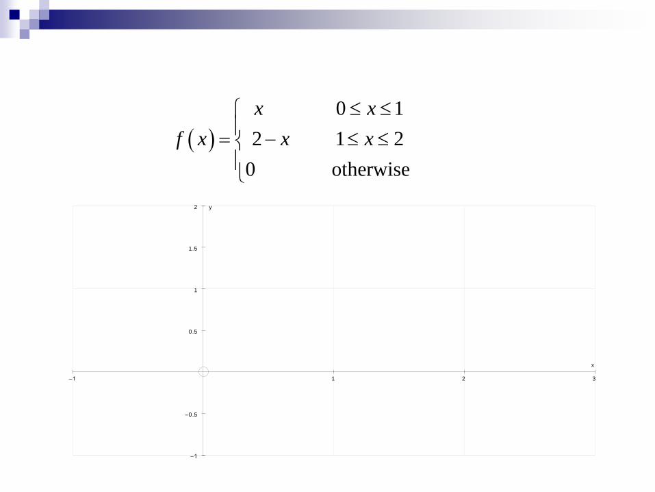
0 1

2 1 2

0 otherwise

x x

f x x x

–1 1 2 3

–1

–0.5

0.5

1

1.5

2

x

y

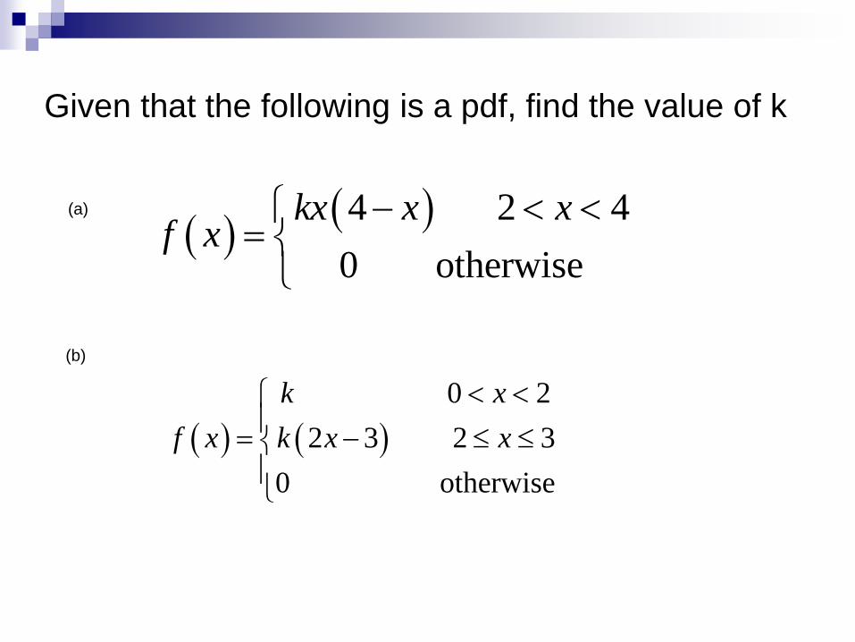
4 2 4

0 otherwise

kx x xf x

0 2

2 3 2 3

0 otherwise

k x

f x k x x

Given that the following is a pdf, find the value of k

(a)

(b)

1

23 3 5

0 otherwise

x xf x

4P x

18

0 4

0 otherwise

x xf x

1 2P x

Example(a)

Find

Find

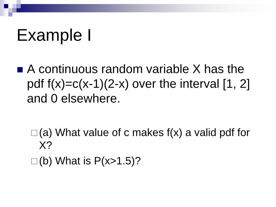
A continuous random variable X has the

pdf f(x)=c(x-1)(2-x) over the interval [1, 2]

and 0 elsewhere.

(a) What value of c makes f(x) a valid pdf for

X?

(b) What is P(x>1.5)?

Example I

Working with CRV Distributions

Median

Mode max. point(s) of f(x)

Mean (expected value)

Variance E(x2)-[E(x)]2 or

m

dxxf )(2

1

dxxfx )(

dxxfx )()( 2

Ex. 1: Mode from Graphs

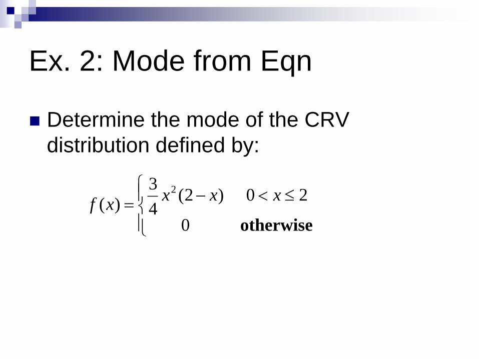
Ex. 2: Mode from Eqn

Determine the mode of the CRV

distribution defined by:

otherwise0

20)2(4

3

)(2 xxx

xf

Ex. 3: Mean & Variance

Determine the mean and variance of the

CRV distribution defined by

otherwise0

31)3)(1(4

3

)(xxx

xf

Ex. 4: Median

Determine the median and lower quartile

of the CRV distribution defined by

otherwise0

21)25(12

1

)(xx

xf

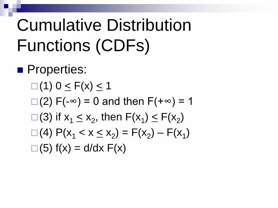
Cumulative Distribution

Functions (CDFs)

Properties:

(1) 0 < F(x) < 1

(2) F(-∞) = 0 and then F(+∞) = 1

(3) if x1 < x2, then F(x1) < F(x2)

(4) P(x1 < x < x2) = F(x2) – F(x1)

(5) f(x) = d/dx F(x)

Ex. 5: Given cdf, work with it ….

A cumulative distribution function is given

by:

(a) Sketch it

(b) find P(x < ¾)

(c) find P(½ < x < ¾)

(d) find P(x > ¼)

11

12

12

10

2

00

)(2

x

xx

xx

x

xF

for

for

for

for

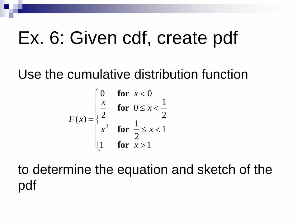
Ex. 6: Given cdf, create pdf

Use the cumulative distribution function

to determine the equation and sketch of the

pdf

11

12

12

10

2

00

)(2

x

xx

xx

x

xF

for

for

for

for

Ex. 7:Given pdf, draw cdf

Given the probability density function of

Draw the corresponding cumulative

probability function

otherwise0

102)(

xxxf