chapter 15 random variables...discrete random variable a discrete random variable x has a countable...
TRANSCRIPT
Chapter 15
Random Variables
click to add subtitles
Objectives:
Define a random variable.
Define a discrete random variable.
Explain what is meant by a probability
distribution or model.
Construct the probability model for a
discrete random variable.
Construct a probability histogram.
Objectives continued,
Expected value
Variance of a random variable
Standard deviation of a random variable
Linear transformations of random
variables
Define a continuous random variable.
Probability distribution for a continuous
random variable.

Random Variables
A random variable is a variable whose value is a numerical outcome of a random phenomenon.
For example: Flip three coins and let Xrepresent the number of heads. X is a random variable.
The sample space S lists the possible values of the random variable X
Random Variable
A random variable assumes a value based
on the outcome of a random event.
We use a capital letter, like X, to denote a
random variable.
A particular value of a random variable will be
denoted with a lower case letter, in this case
x.
Example: P(X = x)
Random Variables
A random variable is a function that
assigns a numerical value to each
simple event in a sample space S.
If these numerical values are only
integers (no fractions or irrational
numbers), it is called a discrete
random variable.
Note that a random variable is
neither random nor a variable - it is a
function with a numerical value, and
it is defined on a sample space.

Random Variables
There are two types of random variables:
Discrete random variables can take one of a
finite number of distinct outcomes.
Example: Number of credit hours
Continuous random variables can take any
numeric value within a range of values.
Example: Cost of books this term

Examples of Random Variables
1. A function whose range is the
number of speeding tickets issued
on a certain stretch of I 95 S.
2. A function whose range is the
number of heads which appear
when 4 dimes are tossed.
3. A function whose range is the
number of passes completed in a
game by a quarterback.
These examples are all discrete
random variables.

Probability Distributions or Model
The simple events in a sample space S could be anything:
heads or tails, marbles picked out of a bag, playing cards.
The point of introducing random variables is to associate
the simple events with numbers, with which we can
calculate.
We transfer the probability assigned to elements or
subsets of the sample space to numbers. This is called
the probability distribution of the random variable X. It is
defined as
p(x) = P(X = x)
Discrete Random Variable
A discrete random variable X has a
countable number of possible values.
For example: Flip three coins and let X
represent the number of heads. X is a
discrete random variable. (In this case, the
random variable X can equal 0, 1, 2, or 3.)
We can use a table to show the probability
distribution of a discrete random variable.
• For example, the number of days it rained in your community during the month of March is an example of a discrete random variable.
• If X is the number of days it rained during the month of March, then the possible values for X are x = 0, 1, 2, 3, …, 31.
Example - Discrete Random
Variable
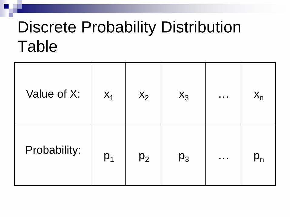
Discrete Probability Distribution
Table
Value of X: x1 x2 x3 … xn
Probability:p1 p2 p3 … pn
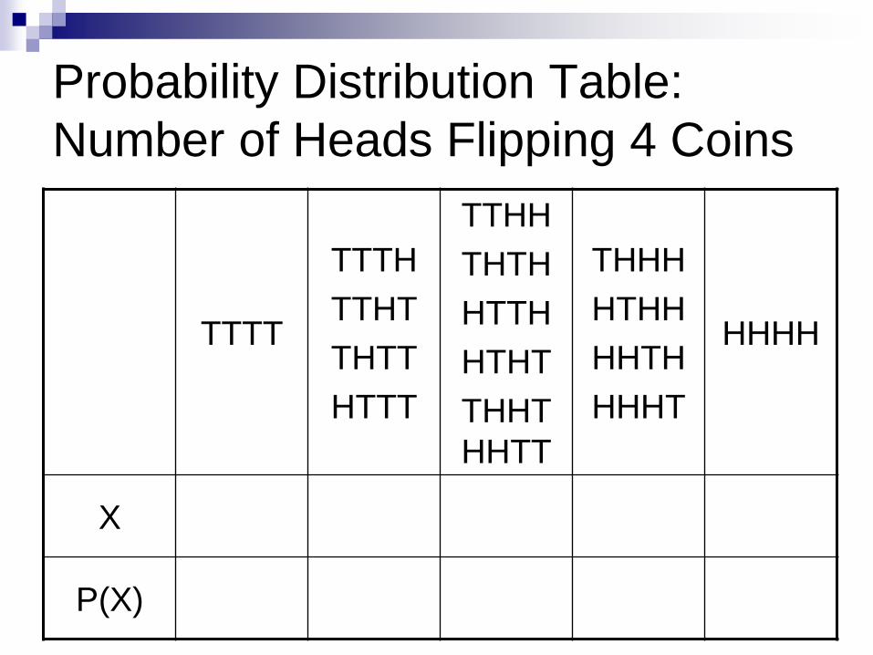
Probability Distribution Table:
Number of Heads Flipping 4 Coins
TTTT
TTTH
TTHT
THTT
HTTT
TTHH
THTH
HTTH
HTHT
THHT
HHTT
THHH
HTHH
HHTH
HHHT
HHHH
X 0 1 2 3 4
P(X) 1/16 4/16 6/16 4/16 1/16
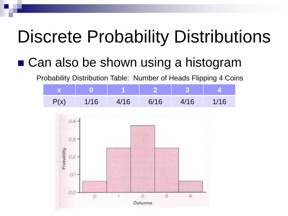
Discrete Probability Distributions
Can also be shown using a histogram
x 0 1 2 3 4
P(x) 1/16 4/16 6/16 4/16 1/16
Probability Distribution Table: Number of Heads Flipping 4 Coins
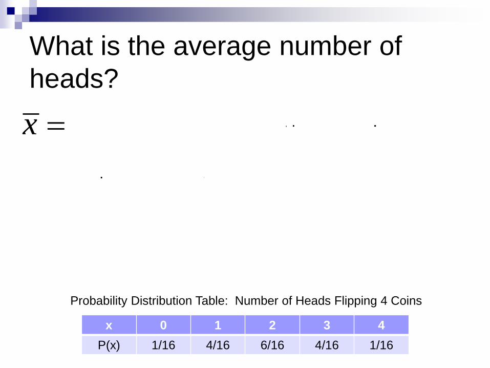
What is the average number of
heads?
61 4 4 116 16 16 16 16
0 4 12 12 416 16 16 16 16
3216
0 1 2 3 4
2
x
Probability Distribution Table: Number of Heads Flipping 4 Coins
x 0 1 2 3 4
P(x) 1/16 4/16 6/16 4/16 1/16
Example - Probability Distributions for
Discrete Random Variables
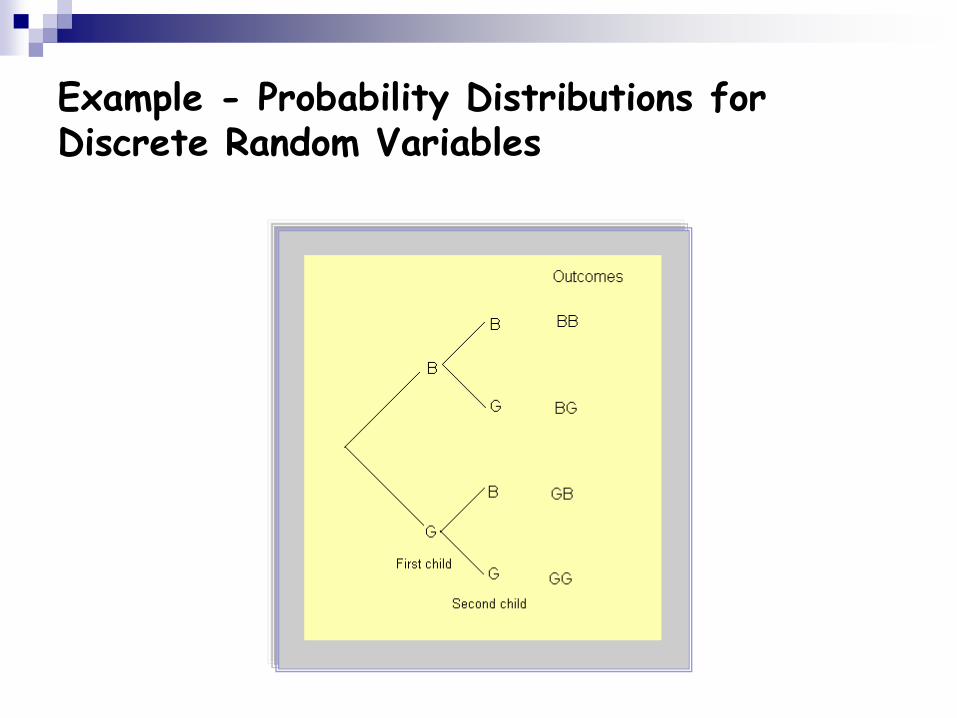
For a two child family, what are the different possible combinations of children?
The sample space was given as S = {BB, BG, GB, GG} and the tree diagram is repeated on the next slide for convenience.
Example - Probability Distributions for Discrete Random Variables
Example - Probability Distributions for Discrete Random Variables
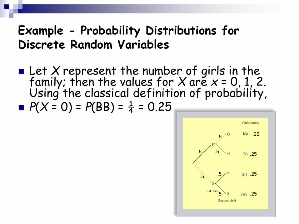
Let X represent the number of girls in the family; then the values for X are x = 0, 1, 2. Using the classical definition of probability,
P(X = 0) = P(BB) = ¼ = 0.25
.5
.5
.5
.5
.5
.5
.25
.25
.25
.25

Example - Probability Distributions for Discrete Random Variables
P(X =1) = P(BG or GB) = P(BG GB) = P(BG) + P(GB) since BG and GB are
mutually exclusive events= ¼ + ¼ = ½ = 0.5
P(X = 2) = P(GG) = ¼ = 0.25
.5
.5
.5
.5
.5
.5
.25
.25
.25
.25
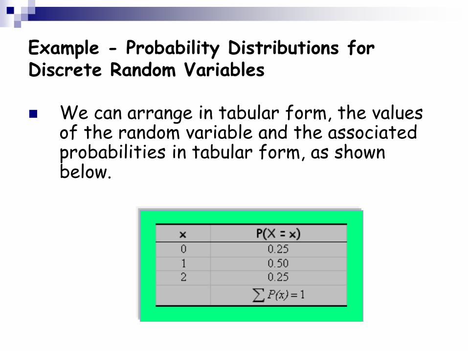
Example - Probability Distributions for Discrete Random Variables
We can arrange in tabular form, the values of the random variable and the associated probabilities in tabular form, as shown below.
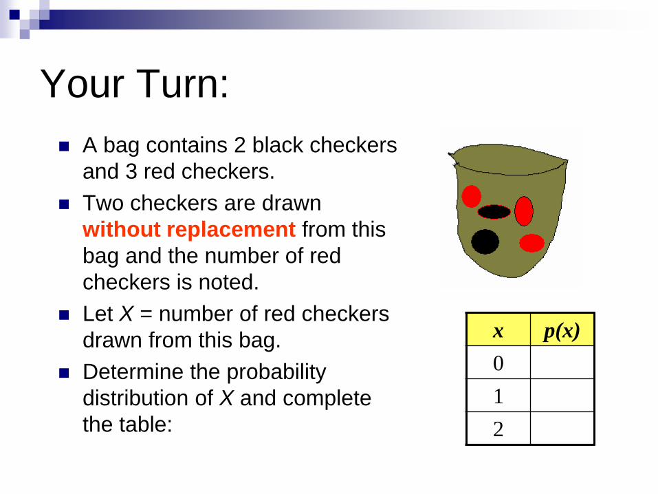
Your Turn:
A bag contains 2 black checkers
and 3 red checkers.
Two checkers are drawn
without replacement from this
bag and the number of red
checkers is noted.
Let X = number of red checkers
drawn from this bag.
Determine the probability
distribution of X and complete
the table:
x p(x)
0
1
2
Continued
x p(x)
0 1/10
1
2
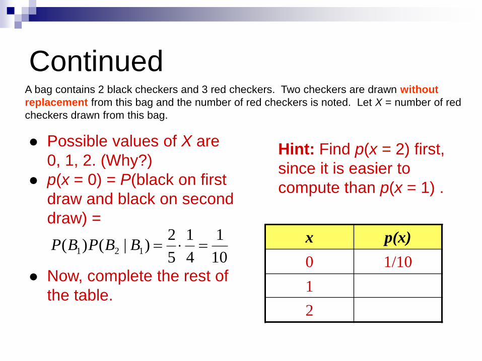
Possible values of X are
0, 1, 2. (Why?)
p(x = 0) = P(black on first
draw and black on second
draw) =
Now, complete the rest of
the table.
Hint: Find p(x = 2) first,
since it is easier to
compute than p(x = 1) .
10
1
4
1
5
2)|()( 121 BBPBP
A bag contains 2 black checkers and 3 red checkers. Two checkers are drawn without
replacement from this bag and the number of red checkers is noted. Let X = number of red
checkers drawn from this bag.

Continued
x p(x)
0 1/10
1 6/10
2 3/10
Possible values of X are
0, 1, 2. (Why?)
p(x = 0) = P(black on first
draw and black on second
draw) =
Now, complete the rest of
the table.
Hint: Find p(x = 2) first,
since it is easier to
compute than p(x = 1) .
10
1
4
1
5
2)|()( 121 BBPBP
A bag contains 2 black checkers and 3 red checkers. Two checkers are drawn without
replacement from this bag and the number of red checkers is noted. Let X = number of red
checkers drawn from this bag.
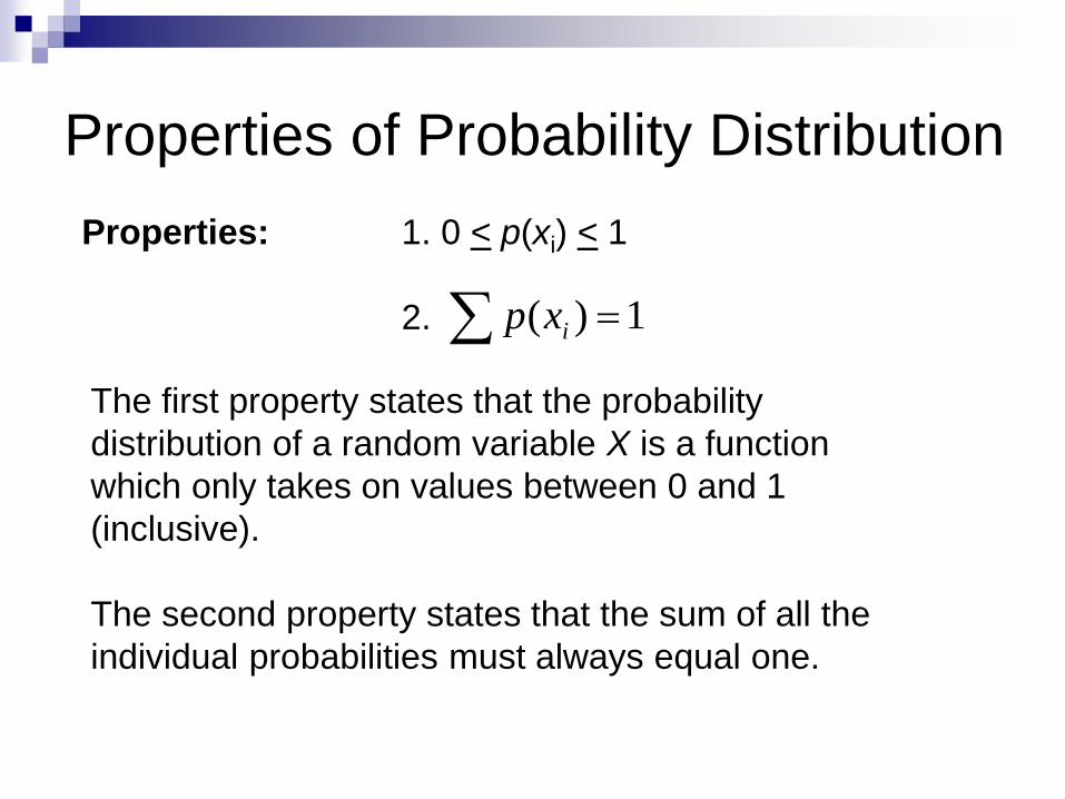
Properties of Probability Distribution
The first property states that the probability
distribution of a random variable X is a function
which only takes on values between 0 and 1
(inclusive).
The second property states that the sum of all the
individual probabilities must always equal one.
Properties: 1. 0 < p(xi) < 1
2. 1)( ixp
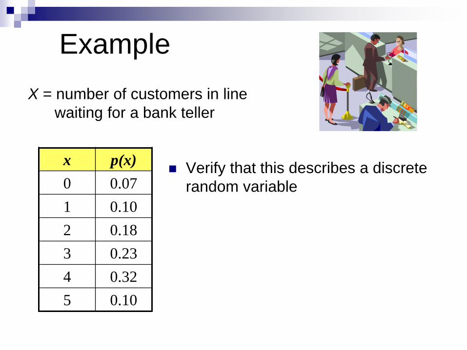
Example
X = number of customers in line
waiting for a bank teller
Verify that this describes a discrete
random variable
x p(x)
0 0.07
1 0.10
2 0.18
3 0.23
4 0.32
5 0.10

Example Solution
X = number of customers in line
waiting for a bank teller
Verify that this describes a discrete
random variable
Solution: Variable X is discrete since
its values are all whole numbers. The
sum of the probabilities is one, and all
probabilities are between 0 and 1
inclusive, so it satisfies the
requirements for a probability
distribution.
x p(x)
0 0.07
1 0.10
2 0.18
3 0.23
4 0.32
5 0.10
Mean / Expected Value
A probability model for a random variable consists of:
The collection of all possible values of a random variable, and
the probabilities that the values occur.
Of particular interest is the value we expect a random variable to take on, notated μ (for population mean) or E(X) for expected value.
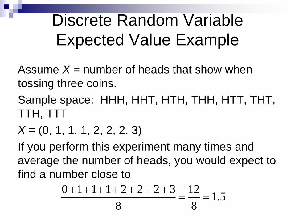
Discrete Random Variable
Expected Value Example
Assume X = number of heads that show when
tossing three coins.
Sample space: HHH, HHT, HTH, THH, HTT, THT,
TTH, TTT
X = (0, 1, 1, 1, 2, 2, 2, 3)
If you perform this experiment many times and
average the number of heads, you would expect to
find a number close to
5.18
12
8
32221110

Expected Value Example (continued)
Notice the outcomes of x = 1 and x = 2 occur three
times each, while the outcomes x = 0 and x = 3
occur once each. We could calculate the average
as
= 1.5
)3(3)2(2)1(1)0(0
8
13
8
32
8
31
8
10
8
323130
pppp
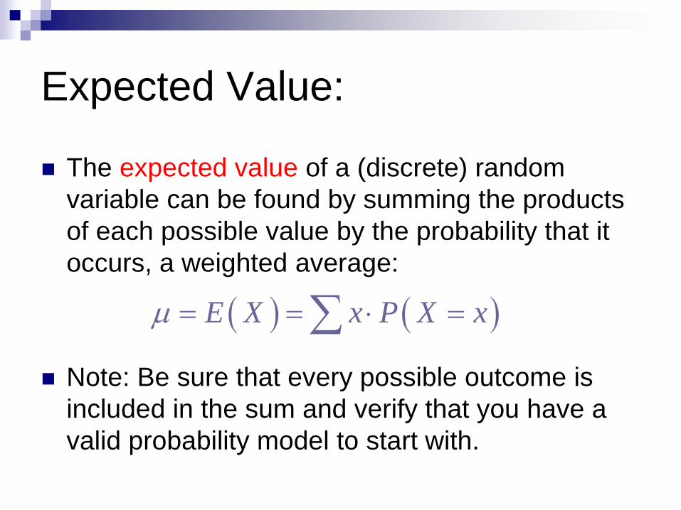
Expected Value:
The expected value of a (discrete) random
variable can be found by summing the products
of each possible value by the probability that it
occurs, a weighted average:
Note: Be sure that every possible outcome is
included in the sum and verify that you have a
valid probability model to start with.
E X x P X x
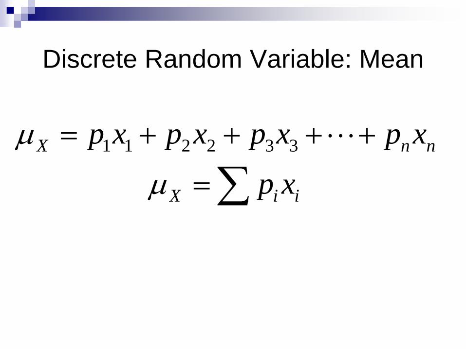
Discrete Random Variable: Mean
1 1 2 2 3 3X n n
X i i
p x p x p x p x
p x
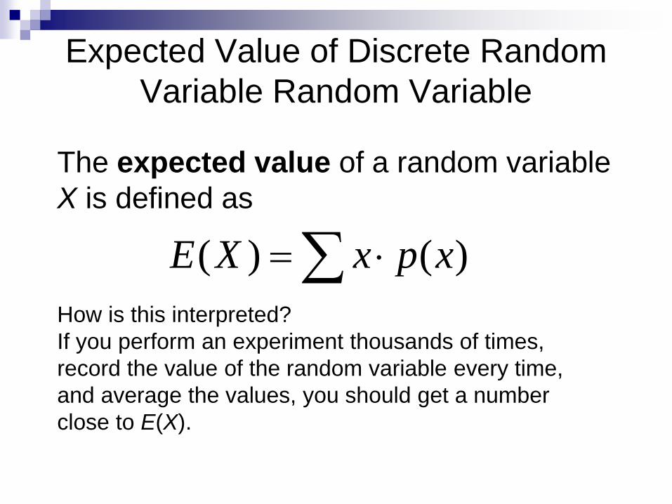
Expected Value of Discrete Random
Variable Random Variable
The expected value of a random variable
X is defined as
)()( xpxXE
How is this interpreted?
If you perform an experiment thousands of times,
record the value of the random variable every time,
and average the values, you should get a number
close to E(X).
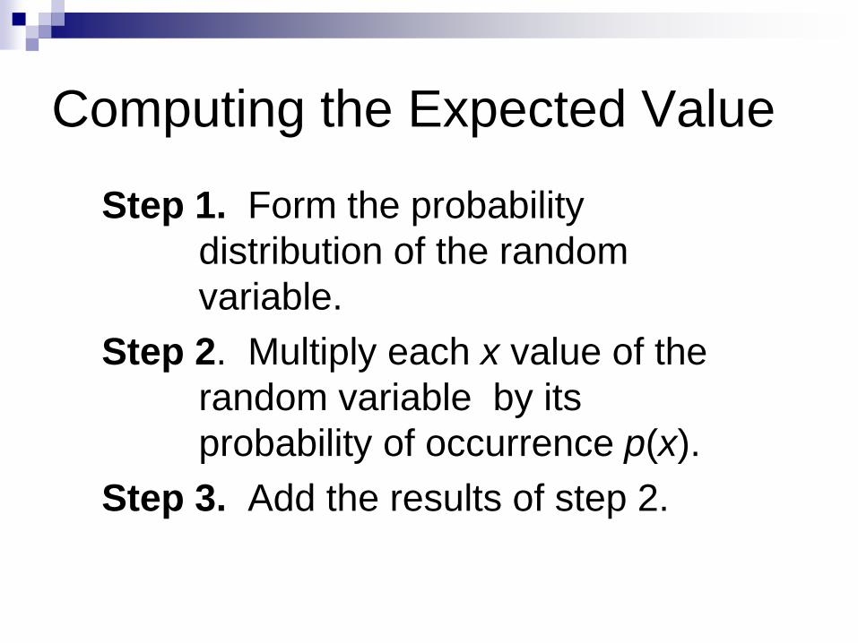
Computing the Expected Value
Step 1. Form the probability
distribution of the random
variable.
Step 2. Multiply each x value of the
random variable by its
probability of occurrence p(x).
Step 3. Add the results of step 2.

Example - Expected Value for a Discrete Random Variable
Example: Find the expected number of girls in a two-child family.
Solution: Let X represent the number of girls in a two-child family.
Use the formula and the information from the probability distribution given on the next slide to compute the expected

Example - Expected Value for a Discrete Random Variable
E(X) = 00.25 + 10.5 + 20.25 = 1. That is, if we sample from a large number of two-
child families, on average, there will be one girl in each family.
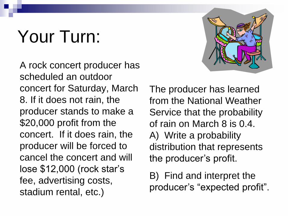
Your Turn:
A rock concert producer has
scheduled an outdoor
concert for Saturday, March
8. If it does not rain, the
producer stands to make a
$20,000 profit from the
concert. If it does rain, the
producer will be forced to
cancel the concert and will
lose $12,000 (rock star’s
fee, advertising costs,
stadium rental, etc.)
The producer has learned
from the National Weather
Service that the probability
of rain on March 8 is 0.4.
A) Write a probability
distribution that represents
the producer’s profit.
B) Find and interpret the
producer’s “expected profit”.

Solution
(A) There are two possibilities: It rains on March 8, or it
doesn’t. Let x represent the amount of money the
producer will make. So, x can either be $20,000 (if it
doesn’t rain) or x = -$12,000 (if it does rain). We can
construct the following table:
x p(x) x ∙ p(x)
rain -12,000 0.4 -4,800
no rain 20,000 0.6 12,000
=7,200
)()( xpxXE

Solution
(B) The expected value is interpreted as a
long-term average. The number $7,200
means that if the producer arranged this
concert many times in identical
circumstances, he would be ahead by
$7,200 per concert on the average. It does
not mean he will make exactly $7,200 on
March 8. He will either lose $12,000 or gain
$20,000.

Statistical Estimation & The Law
of Large Numbers
A SRS should represent the population, so
the sample mean, should be somewhere
near the population mean.
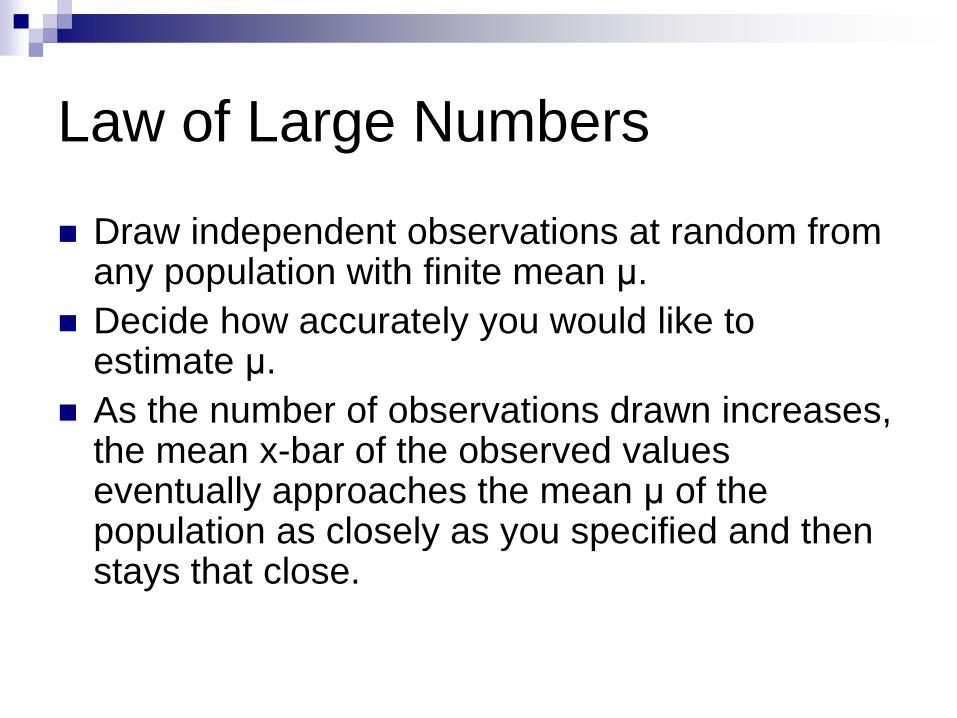
Law of Large Numbers
Draw independent observations at random from any population with finite mean μ.
Decide how accurately you would like to estimate μ.
As the number of observations drawn increases, the mean x-bar of the observed values eventually approaches the mean μ of the population as closely as you specified and then stays that close.


What this means:
The law of large numbers says that the average results
of many independent observations are stable and
predictable (ex; casinos, grocery stores – stock, fast food
restaurants).
Both the rules of probability and the law of large
numbers describe the regular behavior of chance events
in the long run.
How large is a large number?
That depends on the variability of the random outcomes. The
more variable the outcomes, the more trails are needed to
ensure the sample mean is close to the population mean.

Example
The distribution of the heights of all young
women is close to the normal distribution with
mean 64.5 inches and standard deviation 2.5
inches.
What happens if you make larger and larger
samples…
Larger sample size means less variation and the
sample statistics will get closer to the population
parameters 64.5 in and 2.5 in., by the LLN.

Law of Small Numbers or Law of Averages
Most people incorrectly believe in the law
of Small Numbers.
That is, we expect short sequences of
random events to show the kind of
average behavior that in fact appears only
in the long run.
“Runs” of numbers, streaks, hot hand, etc.

A Fair Game
Definition – A game of chance is called fair
if the expected value is zero.
This means that over the long run you will
not win or lose playing the game (you will
brake even).
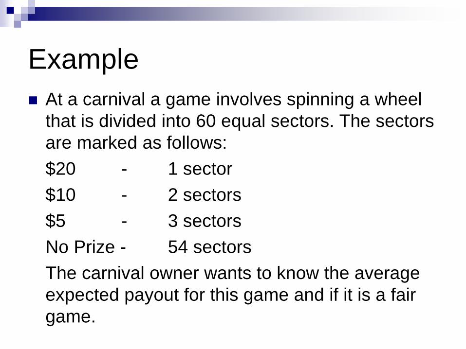
Example
At a carnival a game involves spinning a wheel
that is divided into 60 equal sectors. The sectors
are marked as follows:
$20 - 1 sector
$10 - 2 sectors
$5 - 3 sectors
No Prize - 54 sectors
The carnival owner wants to know the average
expected payout for this game and if it is a fair
game.

Solution
Define the random variable.
Let X = the amount of the payout
Make a probability distribution table.
x $0 $5 $10 $20
P(X=x) 54/60 3/60 2/60 1/60
At a carnival a game involves spinning a wheel that is
divided into 60 equal sectors. The sectors are marked as
follows: $20 - 1 sector
$10 - 2 sectors
$5 - 3 sectors
No Prize - 54 sectors

Find the expected value.
E(x) = $0(54/60) + $5(3/60) + $10(2/60)
+ $20(1/60)
E(x) = $.92
State your conclusion.
In the long run, the carnival owner can
expect a mean payout of about $.92 on
each game played. This is not a fair game.
x $0 $5 $10 $20
P(X=x) 54/60 3/60 2/60 1/60

Example
Refer to the carnival game in the previous
example. Suppose the cost to play the
game is $1. What are a player’s expected
winnings?
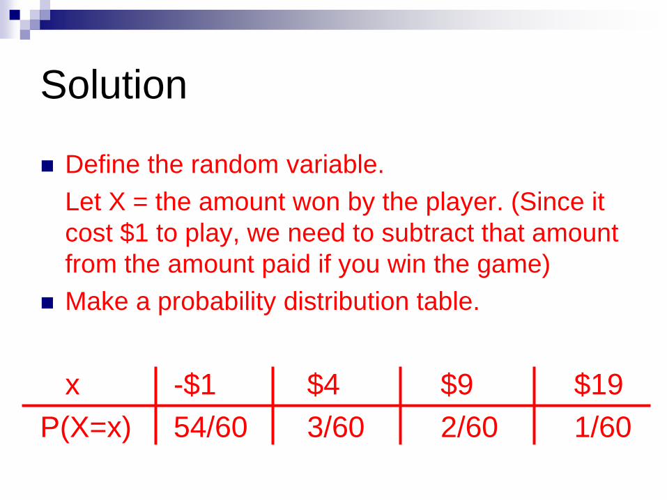
Solution
Define the random variable.
Let X = the amount won by the player. (Since it
cost $1 to play, we need to subtract that amount
from the amount paid if you win the game)
Make a probability distribution table.
x -$1 $4 $9 $19
P(X=x) 54/60 3/60 2/60 1/60

Find the expected value.
E(x) = -$1(54/60) + $4(3/60) + $9(2/60)
+ $19(1/60)
E(x) = -$.08
State your conclusion.
In the long run, the player can expect to
lose about 8 cents for every game he
plays. This is not a fair game.
x -$1 $4 $9 $19
P(X=x) 54/60 3/60 2/60 1/60
Clues for Clarity
When you are asked to calculate the
expected winnings for a game of
chance, don’t forget to take into
account the cost to play the game.

Your Turn:
A game is set up such that you have a 1/5 chance of winning $350 and a 4/5 chance of losing $50. What is your expected gain?
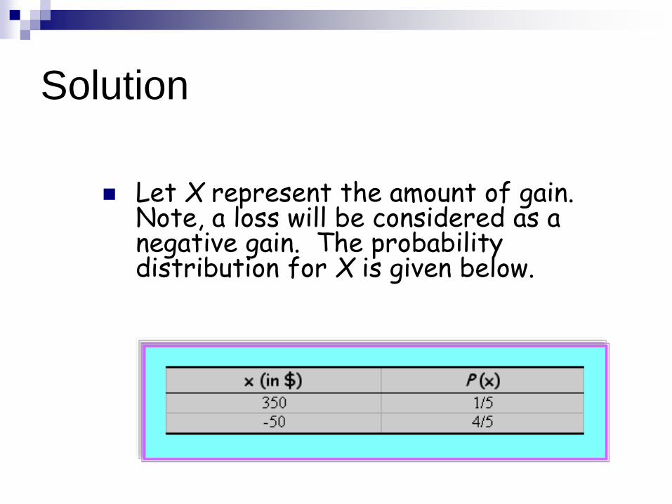
Let X represent the amount of gain. Note, a loss will be considered as a negative gain. The probability distribution for X is given below.
Solution

Solution
Thus, the expected value of the game is E(X) = 3501/5 + (-50)4/5 = $30.
That is, if you play the game a large number of times, on average, you will win $30 per game.
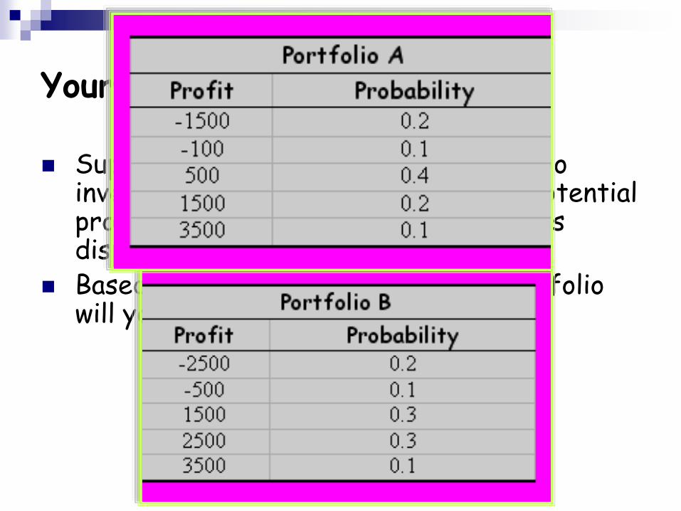
Your Turn:
Suppose you are given the option of two investment portfolios, A and B, with potential profits and the associated probabilities displayed below.
Based on expected profits, which portfolio will you choose?

Solution
Let X represent the profit for portfolio A, and let Y represent the profit for portfolio B. Then,
E(X) = (-1,500)0.2 + (-100)0.1 + 5000.4 + 1,5000.2 + 3,5000.1 = $540
E(Y) = (-2,500)0.2 + (-500)0.1 + 1,5000.3 + 2,5000.3 + 3,5000.1 = $1,000.

Solution
Discussions: Since, E(Y) > E(X), you should invest in portfolio B based on the expected profit.
That is, in the long run, portfolio B will out perform portfolio A.
Thus, under repeated investments in portfolio B, you will, on average, gain $(1,000 – 540) = $460 over portfolio A.
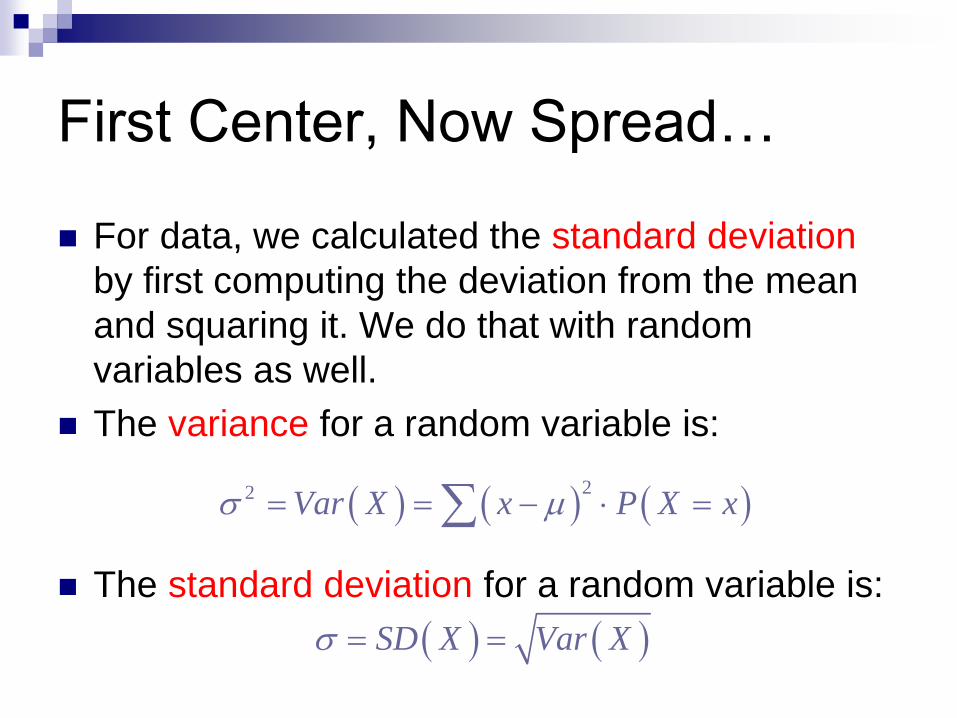
First Center, Now Spread…
For data, we calculated the standard deviation
by first computing the deviation from the mean
and squaring it. We do that with random
variables as well.
The variance for a random variable is:
The standard deviation for a random variable is:
22 Var X x P X x
SD X Var X

Random Variables: Variance
Variance of a discrete random variable is a
weighted (by the probability) average of
the squared deviations (x-μx)2 of the
variable x from its mean μx.
2 2 22
1 1 2 2
22
X x x n n x
X i i x
p x p x p x
p x
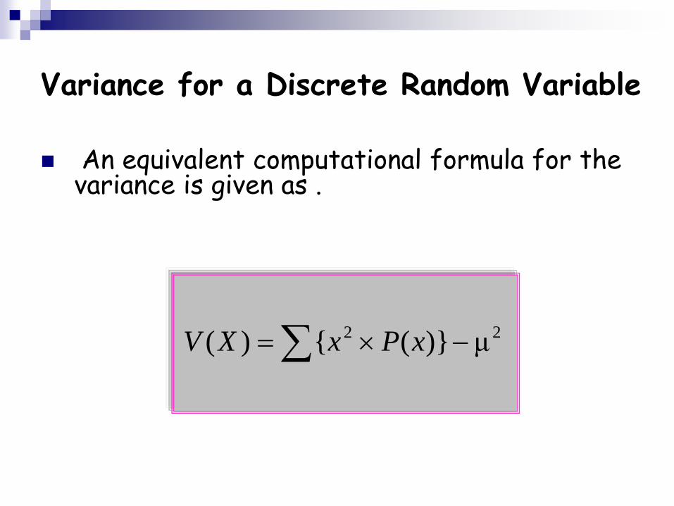
Variance for a Discrete Random Variable
An equivalent computational formula for the variance is given as .
μ)}({)( 22 xPxXV
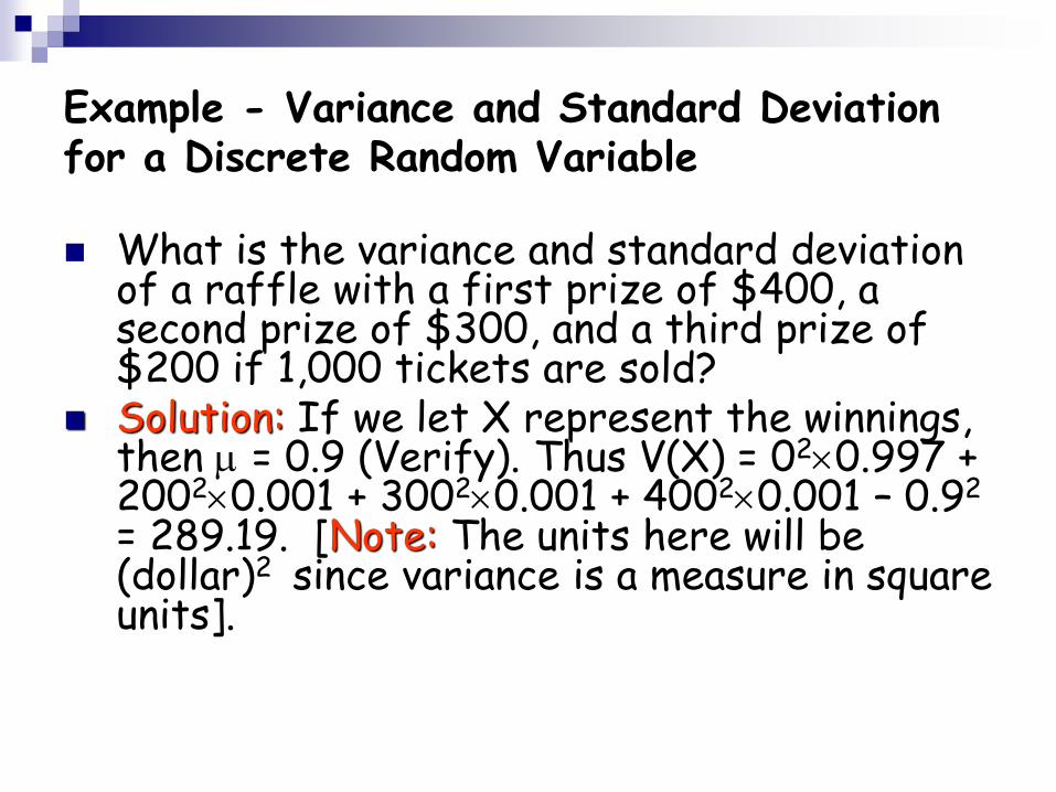
Example - Variance and Standard Deviation for a Discrete Random Variable
What is the variance and standard deviation of a raffle with a first prize of $400, a second prize of $300, and a third prize of $200 if 1,000 tickets are sold?
Solution: If we let X represent the winnings, then = 0.9 (Verify). Thus V(X) = 020.997 + 20020.001 + 30020.001 + 40020.001 – 0.92
= 289.19. [Note: The units here will be (dollar)2 since variance is a measure in square units].
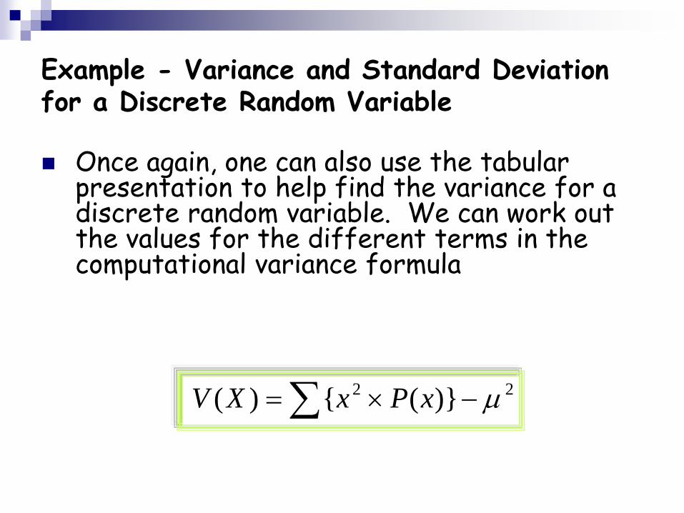
Example - Variance and Standard Deviation for a Discrete Random Variable
Once again, one can also use the tabular presentation to help find the variance for a discrete random variable. We can work out the values for the different terms in the computational variance formula
22 )}({)( xPxXV

Example - Variance and Standard Deviation for a Discrete Random Variable
From the table, V(X) = 290 – 0.92 = 289.19.
)()(
XVXSD SD(X) = 17.01

The total number of cars to be sold next week is
described by the following probability distribution
Determine the expected value and standard deviation
of X, the number of cars sold.
x 0 1 2 3 4
p(x) .05 .15 .35 .25 .20
Your Turn: Car Sales
11.124.1
24.1)20(.)4.24()25(.)4.23()35(.)4.22(
)15(.)4.21()05(.)4.20()()4.2(
40.2)20.0(4)25.0(3)35.0(2)15.0(1)05.0(0)(
222
225
1
22
5
1
X
i
iiX
i
iiX
xpx
xpx

More About Means and Variances
Adding or subtracting a constant from data
shifts the mean but doesn’t change the
variance or standard deviation. The same
is true of random variables.
E(X ± c) = E(X) ± c Var(X ± c) = Var(X)
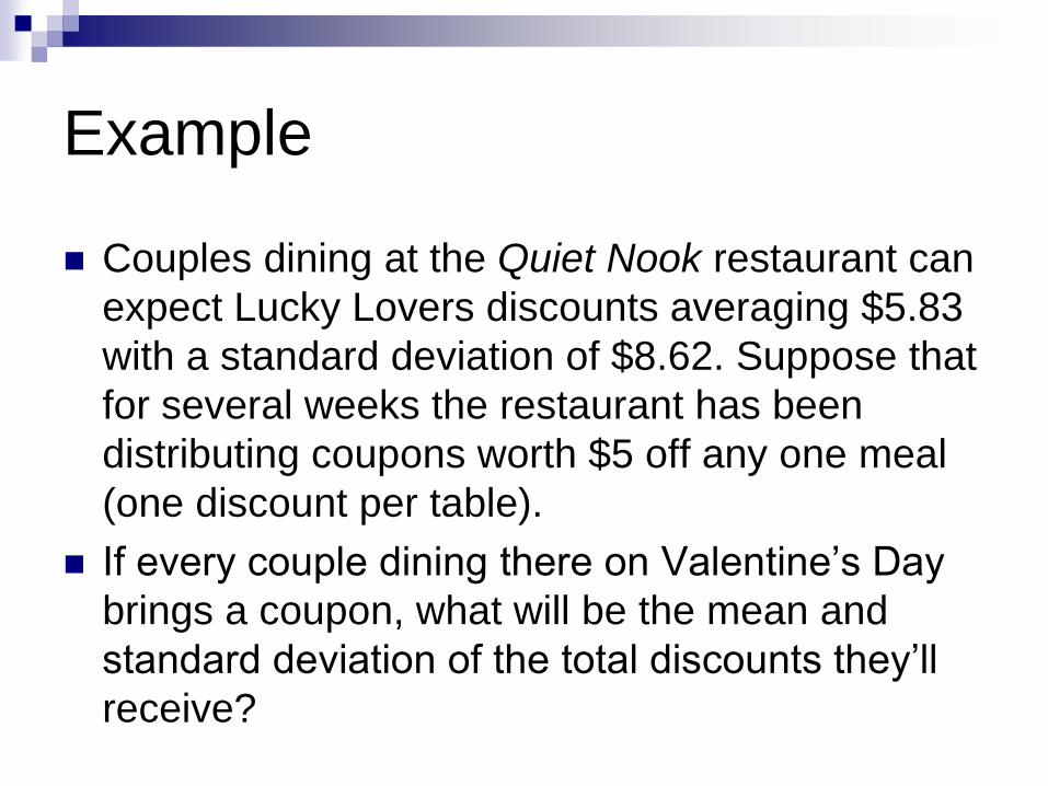
Example
Couples dining at the Quiet Nook restaurant can
expect Lucky Lovers discounts averaging $5.83
with a standard deviation of $8.62. Suppose that
for several weeks the restaurant has been
distributing coupons worth $5 off any one meal
(one discount per table).
If every couple dining there on Valentine’s Day
brings a coupon, what will be the mean and
standard deviation of the total discounts they’ll
receive?

Solution: Couples dining at the Quiet Nook restaurant can expect Lucky
Lovers discounts averaging $5.83 with a standard deviation of $8.62. Suppose that for
several weeks the restaurant has been distributing coupons worth $5 off any one meal
(one discount per table). If every couple dining there on Valentine’s Day brings a coupon,
what will be the mean and standard deviation of the total discounts they’ll receive?
Random variable X = Lucky Lovers Discount, then E(X) = 5.83 and
SD(X) = 8.62 (Var(X) = (8.62)2).
Let the random variable D = total discount (lucky lovers plus the
coupon), then D = X+5.
E(D)
E(D) = E(X+5) = E(X) + 5 = 5.83 + 5 = $10.83
SD(D)
Var(D) = Var(X+5) = Var(X) = (8.62)2
SD(D) = √Var(D) = √(8.62)2 = $8.62
Couples with the coupon can expect total discounts averaging
$10.83 and the standard deviation is still $8.62 (Adding or
subtracting a constant from a random variable, adds or subtracts the
constant from the mean of the random variable, but doesn’t change
the variance or standard deviation.).
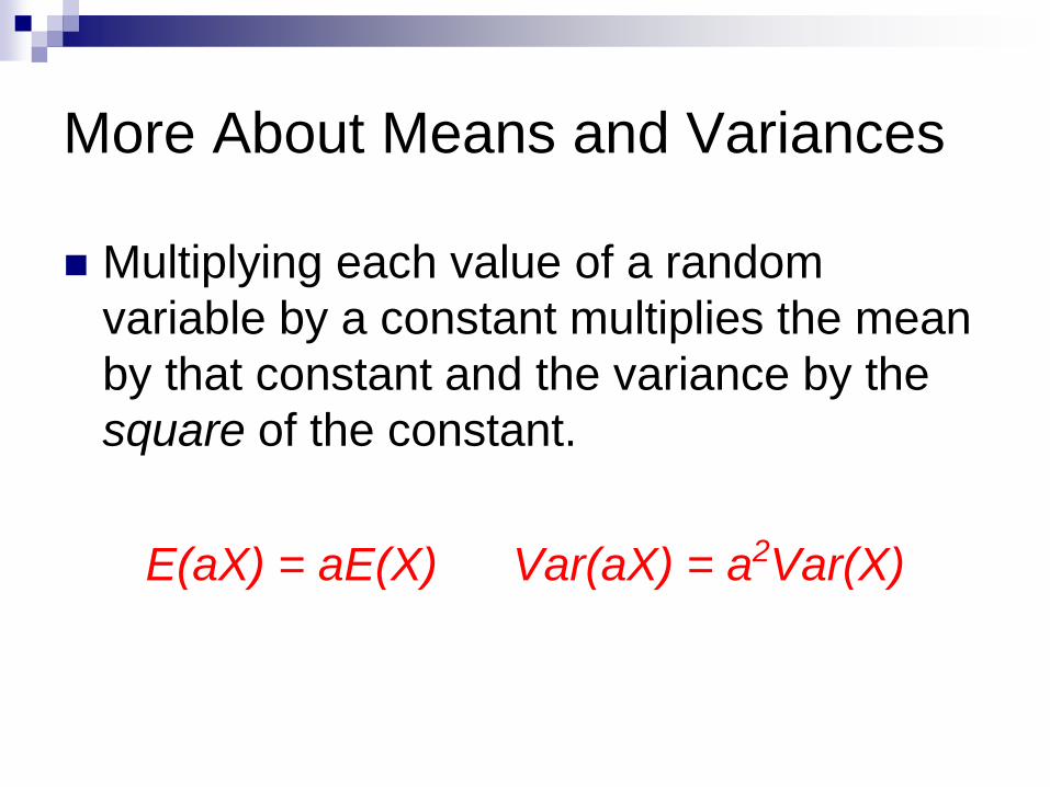
More About Means and Variances
Multiplying each value of a random
variable by a constant multiplies the mean
by that constant and the variance by the
square of the constant.
E(aX) = aE(X) Var(aX) = a2Var(X)

Example
On Valentine’s Day at the Quiet Nook, couples
get a lucky lovers discount averaging $5.83 with
a standard deviation of $8.62. When two couples
dine together on a single check, the resturant
doubles the discount.
What are the mean and standard deviation of
discounts for such foursomes?
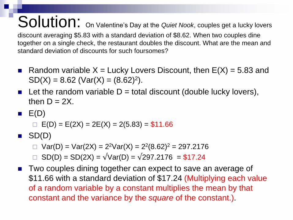
Solution: On Valentine’s Day at the Quiet Nook, couples get a lucky lovers
discount averaging $5.83 with a standard deviation of $8.62. When two couples dine
together on a single check, the restaurant doubles the discount. What are the mean and
standard deviation of discounts for such foursomes?
Random variable X = Lucky Lovers Discount, then E(X) = 5.83 and
SD(X) = 8.62 (Var(X) = (8.62)2).
Let the random variable D = total discount (double lucky lovers),
then D = 2X.
E(D)
E(D) = E(2X) = 2E(X) = 2(5.83) = $11.66
SD(D)
Var(D) = Var(2X) = 22Var(X) = 22(8.62)2 = 297.2176
SD(D) = SD(2X) = √Var(D) = √297.2176 = $17.24
Two couples dining together can expect to save an average of
$11.66 with a standard deviation of $17.24 (Multiplying each value
of a random variable by a constant multiplies the mean by that
constant and the variance by the square of the constant.).

More About Means and Variances
In general,
The mean of the sum of two random variables is the sum of the means.
The mean of the difference of two random variables is the difference of the means.
E(X ± Y) = E(X) ± E(Y)
If the random variables are independent, the variance of their sum or difference is always the sum of the variances.
Var(X ± Y) = Var(X) + Var(Y)
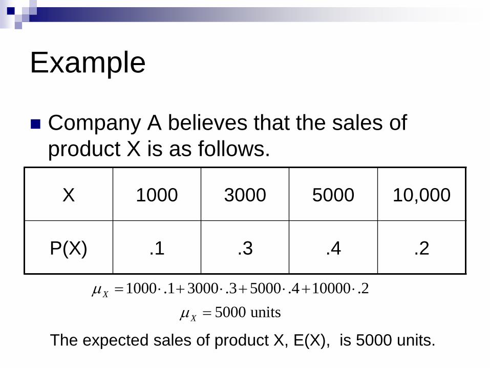
Example
Company A believes that the sales of
product X is as follows.
X 1000 3000 5000 10,000
P(X) .1 .3 .4 .2
1000 .1 3000 .3 5000 .4 10000 .2
5000 units
X
X
The expected sales of product X, E(X), is 5000 units.
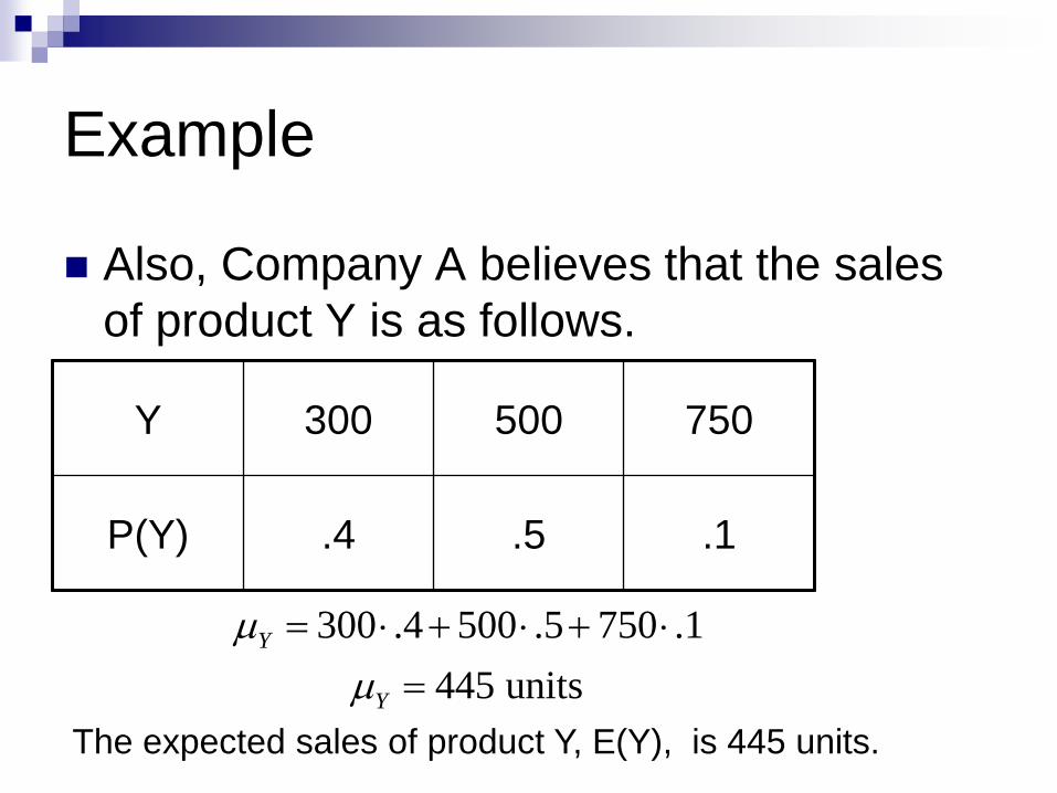
Example
Also, Company A believes that the sales
of product Y is as follows.
Y 300 500 750
P(Y) .4 .5 .1
300 .4 500 .5 750 .1
445 units
Y
Y
The expected sales of product Y, E(Y), is 445 units.
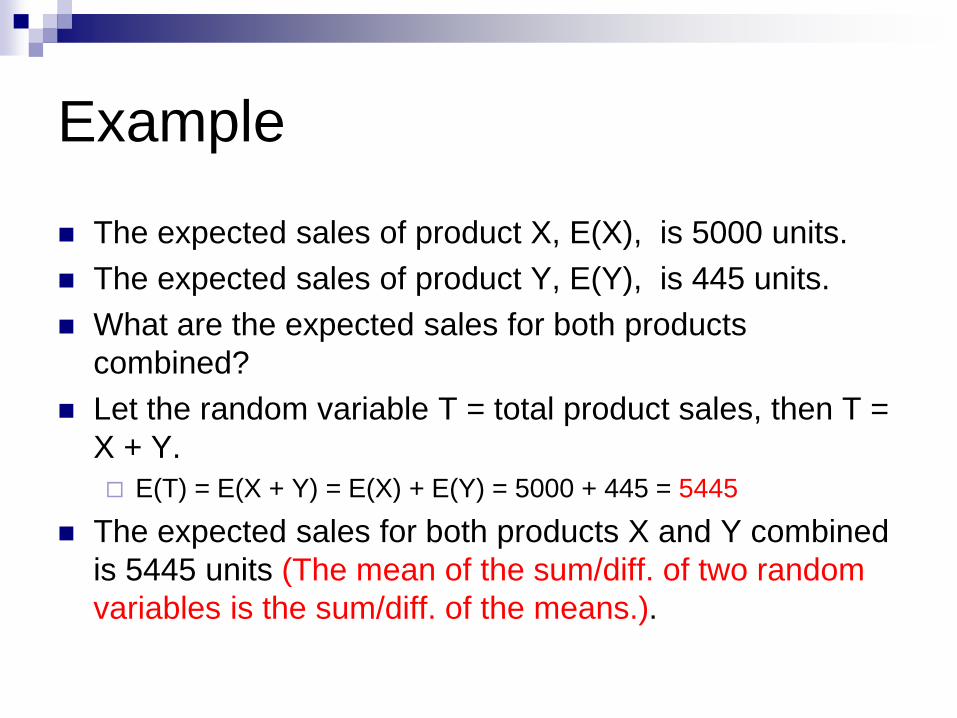
Example
The expected sales of product X, E(X), is 5000 units.
The expected sales of product Y, E(Y), is 445 units.
What are the expected sales for both products
combined?
Let the random variable T = total product sales, then T =
X + Y.
E(T) = E(X + Y) = E(X) + E(Y) = 5000 + 445 = 5445
The expected sales for both products X and Y combined
is 5445 units (The mean of the sum/diff. of two random
variables is the sum/diff. of the means.).

Example
The standard deviation of product X is 2793
units and product Y is 139 units, verify using
your calculator.
What is the difference between the standard
deviations of products X and Y?
Y 300 500 750
P(Y) .4 .5 .1
X 1000 3000 5000 10,000
P(X) .1 .3 .4 .2
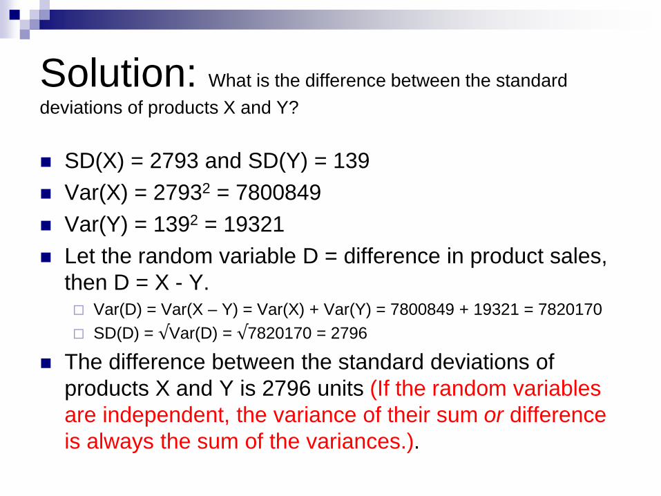
Solution: What is the difference between the standard
deviations of products X and Y?
SD(X) = 2793 and SD(Y) = 139
Var(X) = 27932 = 7800849
Var(Y) = 1392 = 19321
Let the random variable D = difference in product sales,
then D = X - Y. Var(D) = Var(X – Y) = Var(X) + Var(Y) = 7800849 + 19321 = 7820170
SD(D) = √Var(D) = √7820170 = 2796
The difference between the standard deviations of
products X and Y is 2796 units (If the random variables
are independent, the variance of their sum or difference
is always the sum of the variances.).

Continuous Random Variables Random variables that can take on any value in
a range of values are called continuous random variables.
Now, any single value won’t have a probability, but…
Continuous random variables have means (expected values) and variances.
We won’t worry about how to calculate these means and variances in this course, but we can still work with models for continuous random variables when we’re given the parameters.
Continuous Random Variables
Good news: nearly everything we’ve said about
how discrete random variables behave is true of
continuous random variables, as well.
When two independent continuous random
variables have Normal models, so does their
sum or difference.
This fact will let us apply our knowledge of
Normal probabilities to questions about the sum
or difference of independent random variables.

Continuous Random Variable
A continuous random variable X takes
all values in an interval of numbers.
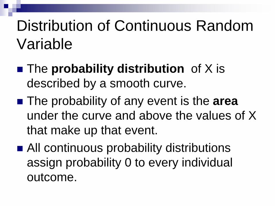
Distribution of Continuous Random
Variable
The probability distribution of X is
described by a smooth curve.
The probability of any event is the area
under the curve and above the values of X
that make up that event.
All continuous probability distributions
assign probability 0 to every individual
outcome.
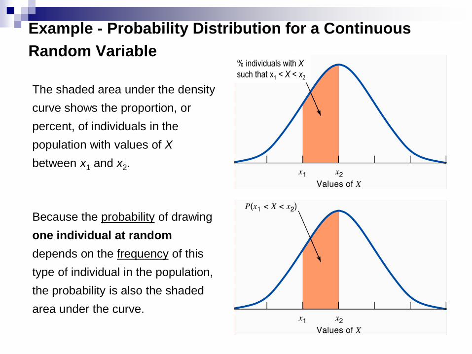
Example - Probability Distribution for a Continuous
Random Variable
Because the probability of drawing
one individual at random
depends on the frequency of this
type of individual in the population,
the probability is also the shaded
area under the curve.
The shaded area under the density
curve shows the proportion, or
percent, of individuals in the
population with values of X
between x1 and x2.
% individuals with X
such that x1 < X < x2

Normal distributions as probability
distributions
Suppose the continuous random variable
X has N(μ,σ) then we can use our normal
distribution tools to calculate
probabilities.
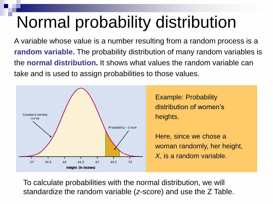
A variable whose value is a number resulting from a random process is a
random variable. The probability distribution of many random variables is
the normal distribution. It shows what values the random variable can
take and is used to assign probabilities to those values.
Example: Probability
distribution of women’s
heights.
Here, since we chose a
woman randomly, her height,
X, is a random variable.
To calculate probabilities with the normal distribution, we will
standardize the random variable (z-score) and use the Z Table.
Normal probability distribution

We standardize normal data by calculating z-scores so that any Normal
curve N(,) can be transformed into the standard Normal curve N(0,1).
Reminder: standardizing N (,)
N(0,1)
→
zy
N(64.5, 2.5)
Standardized height (no units)
( )yz

Previously, we wanted to calculate the proportion of individuals in the population
with a given characteristic.
N (µ, ) = N (64.5, 2.5)
Distribution of women’s heights ≈
Example: What's the proportion
of women with a height between
57" and 72"?
That’s within ± 3 standard
deviations of the mean , thus
that proportion is roughly 99.7%.
Since about 99.7% of all women have heights between 57" and 72", the chance
of picking one woman at random with a height in that range is also about 99.7%.
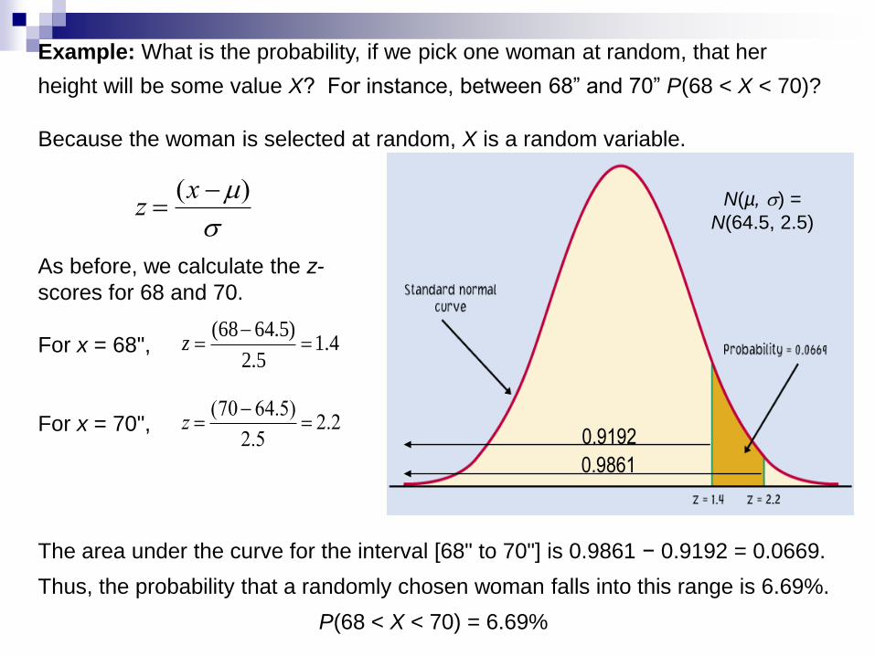
Example: What is the probability, if we pick one woman at random, that her
height will be some value X? For instance, between 68” and 70” P(68 < X < 70)?
Because the woman is selected at random, X is a random variable.
As before, we calculate the z-
scores for 68 and 70.
For x = 68",
For x = 70",
z (x )
4.15.2
)5.6468(
z
z (70 64.5)
2.5 2.2
The area under the curve for the interval [68" to 70"] is 0.9861 − 0.9192 = 0.0669.
Thus, the probability that a randomly chosen woman falls into this range is 6.69%.
P(68 < X < 70) = 6.69%
0.9861
0.9192
N(µ, ) =
N(64.5, 2.5)
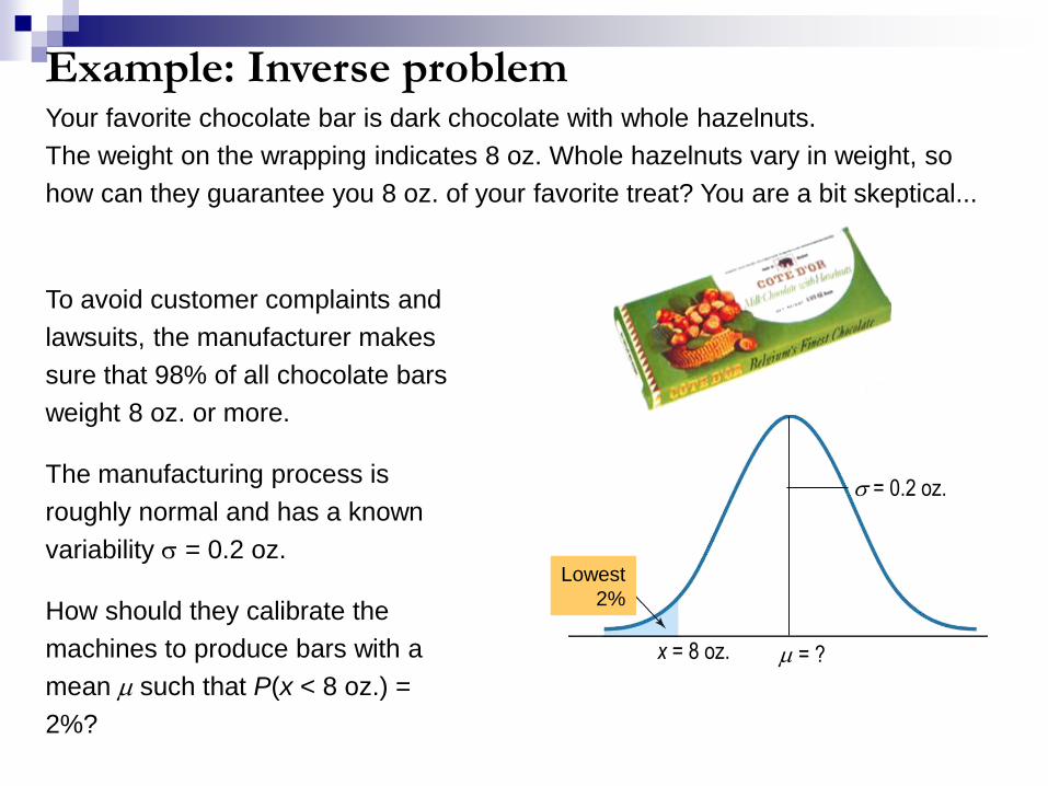
Example: Inverse problemYour favorite chocolate bar is dark chocolate with whole hazelnuts.
The weight on the wrapping indicates 8 oz. Whole hazelnuts vary in weight, so
how can they guarantee you 8 oz. of your favorite treat? You are a bit skeptical...
To avoid customer complaints and
lawsuits, the manufacturer makes
sure that 98% of all chocolate bars
weight 8 oz. or more.
The manufacturing process is
roughly normal and has a known
variability = 0.2 oz.
How should they calibrate the
machines to produce bars with a
mean such that P(x < 8 oz.) =
2%?
= ?x = 8 oz.
Lowest
2%
= 0.2 oz.
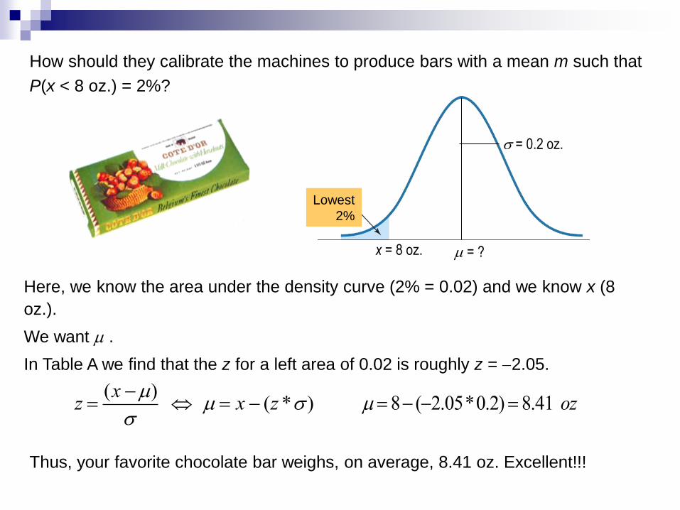
How should they calibrate the machines to produce bars with a mean m such that
P(x < 8 oz.) = 2%?
z (x )
x (z*)
8 (2.05*0.2) 8.41 oz
Here, we know the area under the density curve (2% = 0.02) and we know x (8
oz.).
We want .
In Table A we find that the z for a left area of 0.02 is roughly z = 2.05.
Thus, your favorite chocolate bar weighs, on average, 8.41 oz. Excellent!!!
= ?x = 8 oz.
Lowest
2%
= 0.2 oz.

Slide 16 - 90
What Can Go Wrong?
Probability models are still just models.
Models can be useful, but they are not reality.
Question probabilities as you would data, and think about the assumptions behind your models.
If the model is wrong, so is everything else.
What Can Go Wrong? (cont.)
Don’t assume everything’s Normal.
Watch out for variables that aren’t independent:
You can add expected values for any two random variables, but
you can only add variances of independentrandom variables.
What Can Go Wrong?
Don’t forget: Variances of independent random
variables add. Standard deviations don’t.
Don’t forget: Variances of independent random
variables add, even when you’re looking at the
difference between them.
Don’t forget: Don’t write independent instances
of a random variable with notation that looks like
they are the same variables.
What have we learned?
We know how to work with random variables. We can use a probability model for a discrete random
variable to find its expected value and standard deviation.
The mean of the sum or difference of two random variables, discrete or continuous, is just the sum or difference of their means.
And, for independent random variables, the variance of their sum or difference is always the sum of their variances.
What have we learned?
Normal models are once again special.
Sums or differences of Normally distributed
random variables also follow Normal models.

Assignment
Pg. 383 – 387:#1, 3, 5, 15, 19, 21, 25, 27,
33, 37
Read Ch-17 pg. 388 - 400