rainfall nowcasting by at site stochastic model p.r.a.i.s.e

Hydrol. Earth Syst. Sci., 11, 1341–1351, 2007www.hydrol-earth-syst-sci.net/11/1341/2007/© Author(s) 2007. This work is licensedunder a Creative Commons License.

Hydrology andEarth System

Sciences

Rainfall nowcasting by at site stochastic model P.R.A.I.S.E.

B. Sirangelo, P. Versace, and D. L. De Luca

Dipartimento di Difesa del Suolo, Universita della Calabria – Rende, Italy

Received: 8 January 2007 – Published in Hydrol. Earth Syst. Sci. Discuss.: 29 January 2007Revised: 18 April 2007 – Accepted: 28 April 2007 – Published: 15 May 2007

Abstract. The paper introduces a stochastic model to fore-cast rainfall heights at site: the P.R.A.I.S.E. model (Predic-tion of Rainfall Amount Inside Storm Events). PRAISE isbased on the assumption that the rainfall heightHi+1 ac-cumulated on an interval1t between the instantsi1t and(i+1)1t is correlated with a variableZ(ν)

i , representingantecedent precipitation. The mathematical background is

given by a joined probability densityfHi+1,Z

(ν)i

(hi+1, z

(ν)i

)in which the variables have a mixed nature, that is a finiteprobability in correspondence to the null value and infinites-imal probabilities in correspondence to the positive values.As study area, the Calabria region, in Southern Italy, was se-lected, to test performances of the PRAISE model.

1 Introduction

Rainfall is the main input for all hydrological models suchas, for example, rainfall-runoff models and for forecastinglandslides induced by precipitation. In the last few yearscatastrophic rainfall events have occurred in the Mediter-ranean area, leading to floods, flash floods and shallow land-slides (debris and mud flows). Consequently there is theneed for the implementation of forecasting systems able topredict meteorological conditions leading to disastrous oc-currences. Nowadays, for achieving this goal, meteorolog-ical and stochastic models are used. The former (Chuanget al., 2000; Palmer et al., 2000; Untch et al., 2006) canbe viewed as valid qualitative-quantitative rainfall forecast-ing tools at 24, 48 and 72 h (of course, at these forecastinghorizons an absolute precision is not required, but rather anorder of magnitude) when these phenomena occur on a con-siderable spatial scale. Nevertheless, they cannot yet be re-garded as providers of quantitative rainfall forecasts in the

Correspondence to:D. L. De Luca([email protected])

short term (6–12 h) to be used directly for forecasting sys-tems, since the quantitative forecasting of precipitation, onthe time and space scales of the hydrological phenomena, hasnot yet achieved the degree of precision necessary to avoideither the non-forecasting of exceptional small-scale situa-tions or the issuing of unwarranted alarms. Consequently,in order to perform short term real-time rainfall forecasts forsmall basins (i.e. with size ranging 100–1000 km2), tempo-ral stochastic models appear more competitive. Stochasticprocesses are widely used in hydrological variables forecast-ing (Waymire and Gupta, 1981; Georgakakos and Kavvas,1987; Foufoula-Georgiou and Georgakakos, 1988) and, asregards at-site models, precipitation models can be catego-rized into two broad types: “discrete time-series models” and“point processes models”. Models of the former type, that in-clude AutoRegressive Stochastic Models (Box and Jenkins,1976; Salas et al., 1980; Brockwell and Davis, 1987; Bur-lando et al., 1993; Hipel and McLeod, 1994; Burlando etal., 1996; Toth et al., 2000), describe the rainfall process atdiscrete time steps, are not intermittent and therefore can beapplied for describing the “within storm” rainfall. Modelsof the latter type (Lewis, 1964; Kavvas and Delleur, 1981;Smith and Karr, 1983; Rodriguez-Iturbe et al., 1984, 1987;Rodriguez-Iturbe, 1986; Cowpertwait et al., 1996; Sirangeloand Iiritano, 1997; Calenda and Napolitano, 1999; Montanariand Brath, 1999; Cowpertwait, 2004) are continuous time se-ries models, are intermittent and therefore can simulate inter-storm periods also.

In the present work, a special kind of AutoRegressivemodel, named PRAISE (Prediction of Rainfall Amount In-side Storm Events), is described. It can be considered as asimple and useful tool for at site nowcasting precipitation,especially for applications in rainfall-runoff models, regard-ing small basins, and forecasting landslides, induced by rain-fall, models. The paper is structured in three sections, ex-cluding the introduction: in Sect. 2 the theoretical bases ofthe stochastic model are illustrated; while in Sect. 3 model

Published by Copernicus GmbH on behalf of the European Geosciences Union.

1342 B. Sirangelo et al.: A new stochastic model to nowcast rainfall at site

calibration is shown; finally, Sect. 4 concerns the applicationof the model to the raingauge network of the Calabria region,in Southern Italy, with particular regard to the Cosenza rain-gauge.

2 The PRAISE model

In the PRAISE model, the rainfall heightshn, cumulated overintervals] (n−1) 1t, n1t ], are considered as a realisation ofa weakly stationary stochastic process with discrete param-eter{Hn; n∈I }, whereI indicates the integer numbers. TheHn are non-negative random variables of mixed type, withfinite probability on zero value and infinitesimal probabilityon positive values. In the following the instanti1t=t0 is as-sumed as current time, so that the observed rainfall heightsare with subscripts less or equal toi and the probabilistic pre-diction will be referred to the rainfall heights with subscriptsgreater thani.

The main feature of the approach suggested in thePRAISE model is the identification of a random vari-able Z

(ν)i , a suitable function of theν random variables

Hi, Hi−1, ..., Hi−ν+1, such that its stochastic dependencewith the random variableHi+1 describes the whole correl-ative structure of the process{Hn; n∈I }. Two steps are re-quired to identifyZ(ν)

i :a) the individuation of the process “memory” extensionν;b) the optimal choice of the function depending on the ran-

dom variablesHi, Hi−1, ..., Hi−ν+1 definingZ(ν)i .

After this, the PRAISE model provides the identification

of the joint probability densityfHi+1,Z

(ν)i

(hi+1, z

(ν)i

)and its

utilisation for the real time forecasting of rainfall heights dur-ing a storm event.

2.1 Extension of the “memory”

In the PRAISE model, the linear stochastic dependence be-tween the random variableHi+1 and the generic antecedentrandom variablesHi−j , j=0, 1, 2, ..., is considered negligi-ble when the correspondent sample coefficient of partial au-tocorrelation results less than a fixed value close to zero. Theresults given by this approach are similar to the more rigor-ous and less simple general method, in which the absenceof a linear stochastic dependence should be tested verifyingthat the sample coefficient of partial autocorrelation, betweensuch random variables, exhibits a value inside a confidenceinterval, which does not permit the rejection of the null valuehypothesis for the correspondent theoretical quantity.

In order to determine the extension of the “memory”for the process{Hn; n∈I }, the absence of significant par-tial autocorrelation must be checked for increasing valuesof ν. For each value ofν must be verified the negligibil-ity of all the sample coefficients of partial autocorrelationρHi+1 Hi−ν+1−m·Hi ... Hi−ν+1 characterised by a couple of pri-

mary subscriptsHi+1, Hi−ν; Hi+1, Hi−ν−1; ... and by sec-ondary subscriptsHi, Hi−1, ... , Hi−v+1.

Pratically, evaluation ofρHi+1 Hi−ν+1−m·Hi ... Hi−ν+1 must beperformed using the sample coefficients of partial autocor-relationrHi+1Hi−ν+1−m·Hi ...Hi−ν+1, m=1, 2, ..., obtained by anobserved sampleh1, h2, ... , hN of rainfall heights cumu-lated over time intervals of duration1t , after estimation ofautocorrelationρk by sample autocorrelation coefficientsrk(Kendall and Stuart, 1969); for the hypothesis of weakly sta-tionary process, autocorrelation depends only on lagk.

Finally, to estimate the extension of the “memory”, a sim-ple way can be obtained introducing the sample maximumabsolute scattering:

χr (ν) = max1≤m<∞

∣∣ rHi+1Hi−ν+1−m·Hi ... Hi−ν+1

∣∣ m=1, 2, ... (1)

The extension of the process “memory” can be assumedequal to the minimum value ofν for whichχr (ν) results lessthan a fixed critical valueχr,cr .

2.2 Structure of the random variableZ(ν)i

The criterion adopted in the PRAISE model to define a func-tional dependence between the random variableZ

(ν)i and

the random variablesHi, Hi−1, ..., Hi−ν+1 is the maximi-sation of the coefficient of linear correlationρ

Hi+1,Z(ν)i

be-

tween the sameZ(ν)i and the random variableHi+1. This

choice allows, once identified the joint probability den-

sity fHi+1,Z

(ν)i

(hi+1, z

(ν)i

), the best prediction of rainfall

heightsHi+1 during a storm event. If a functional relation-ship Z

(ν)i =f01 ( Hi, Hi−1, ... , Hi−ν+1) satisfies the crite-

rion here adopted, then all the functions:

fab ( Hi, Hi−1, ... , Hi−ν+1)

= a + b f01 ( Hi, Hi−1, ... , Hi−ν+1) (2)

with a and b generic constants, satisfy the same criterion.In other words, the criterion of maximisation of the coeffi-cient of linear correlation betweenZ(ν)

i andHi+1 identifies a“class of functions”, defined by Eq. (2), with all the membersequivalent for the purposes of the suggested model.

As regards the analytical form of the relationship linkingZ

(ν)i to Hi, Hi−1, ... , Hi−ν+1, the more suitable choice is,

clearly, the linear function:

Z(ν)i = β +

ν−1∑j=0

α′

jHi−j (3)

In this condition, in fact, the coefficients of the linear re-lationship that maximisesρ

Hi+1,Z(ν)i

are simply the coef-

ficients of the linear partial regression amongHi+1 andHi, Hi−1, ..., Hi−ν+1:

E(Hi+1 | H ′

i , H ′

i−1, ..., H ′

i−ν+1

)= µH +

ν−1∑j=0

α′

jH′

i−j (4)

Hydrol. Earth Syst. Sci., 11, 1341–1351, 2007 www.hydrol-earth-syst-sci.net/11/1341/2007/

B. Sirangelo et al.: A new stochastic model to nowcast rainfall at site 1343

where E (.) is the expected value operator,µH =E (Hn),constant value for everyn because of the hypoth-esis of weakly stationary stochastic process, andH ′

i =Hi−µH , H ′

i−1=Hi−1−µH , H ′

i−ν+1=Hi−ν+1−µH .Theα′

j coefficients are evaluated as:

α′

j = −λ(ν+1)1(j+2)

/λ

(ν+1)11 (5)

whereλ(ν+1)1(j+2) e λ

(ν+1)11 are the cofactors of the Laurent ma-

trix:

[3(ν+1)

]=

1 ρ1 ρ2 ... ρν

ρ1 1 ρ1 ... ρν−1ρ2 ρ1 1 ... ρν−2... ... ... ... ...

ρν ρν−1 ρν−2 ... 1

(6)

These coefficients can be readily evaluated utilising again anobserved sampleh1, h2, ... , hN of rainfall heights cumu-lated over time intervals of duration1t . However, it shouldbe highlighted that, as a consequence of the non-negativecharacter of the involved random variables, the coefficientsα′

j must satisfy the conditionsα′

j≥0 for j=0, 1, ... , ν−1.Moreover, the coefficientsα′

j identify, among all the possi-ble linear combinations ofHi, Hi−1, ..., Hi−ν+1 variables,the one which maximizes the linear correlation coefficientwith Hi+1.

Then, definition ofZ(ν)i variable is very simple: letZ(ν)

∗i

be a variable defined as:

Z(ν)∗i = µH +

ν−1∑j=0

α′

jH′

i−j (7a)

it can be noted that it is equal to the conditional expectedvalue E

(Hi+1 | H ′

i , H ′

i−1, ..., H ′

i−ν+1

); rewriting Eq. (7a)

utilising Hi, Hi−1, ..., Hi−ν+1:

Z(ν)∗i =

ν−1∑j=0

α′

jHi−j +

(1 −

ν−1∑j=0

α′

j

)µH (7b)

and introducing the standardised coefficients:

αj = α′

j

/ν−1∑κ=0

α′κ (8)

for which the conditions 0<αj≤1, for j=0, 1, ... , ν−1, andν−1∑j=0

αj=1 are respected,Z(ν)∗i can be expressed as:

Z(ν)∗i =

ν−1∑k=0

α′

k

ν−1∑j=0

αjHi−j +

(1 −

ν−1∑j=0

α′

j

)µH (9)

DefiningZ(ν)i as:

Z(ν)i =

ν−1∑j=0

αjHi−j (10)

it is simple to verify thatZ(ν)∗i andZ

(ν)i variables are con-

nected by a linear transformation, identifying a class of func-tion, defined by Eq. (2). Consequently the correlation coeffi-cientρ

Hi+1, Z(ν)i

is equal toρHi+1, Z

(ν)∗i

.

Equation (10) shows that the random variableZ(ν)i can be

regarded as a weighted average of theν antecedent rainfallheights with weights expressed by the coefficientsαj .

2.3 Joint probability densityfHi+1,Z

(ν)i

(hi+1, z

(ν)i

)Keeping in mind the character of random variable of mixedtype for Hi+1 and, therefore, forZ(ν)

i , the joint probability

densityfHi+1,Z

(ν)i

(hi+1, z

(ν)i

)must be written in the form:

fHi+1,Z

(ν)i

(hi+1, z

(ν)i

)= p·,·δ (hi+1) δ

(z(ν)i

)+p+,·f

(+,·)Hi+1,0

(hi+1) δ(z(ν)i

)+p·,+f

(·,+)

0,Z(ν)i

(z(ν)i

)δ (hi+1)

+p+,+f(+,+)

Hi+1,Z(ν)i

(hi+1, z

(ν)i

)(11)

where δ (.) is Dirac’s delta function,p·,·, p+,·, p·,+ and

p+,+ indicate, respectively, Pr[Hi+1=0 ∩ Z

(ν)i =0

],

Pr[Hi+1>0 ∩ Z

(ν)i =0

], Pr

[Hi+1=0 ∩ Z

(ν)i >0

]and Pr

[Hi+1>0 ∩ Z

(ν)i >0

], with, obviously,

p·,·+p+,·+p·,++p+,+=1, and:

f(+,+)

Hi+1,Z(ν)i

(hi+1, z

(ν)i

)· dhi+1dz

(ν)i =

Pr[hi+1 ≤ Hi+1 < hi+1 + dhi+1 ∩

z(ν)i ≤ Z

(ν)i < z

(ν)i + dz

(ν)i | Hi+1 > 0 ∩ Z

(ν)i > 0

](12)

f(+,·)Hi+1,0

(hi+1) · dhi+1 =

Pr[hi+1 ≤ Hi+1 < hi+1 +dhi+1| Hi+1>0 ∩ Z

(ν)i =0

](13)

f(·,+)

0,Z(ν)i

(z(ν)i

)·dz

(ν)i =

Pr[z(ν)i ≤Z

(ν)i <z

(ν)i +dz

(ν)i

∣∣∣Hi+1 = 0 ∩ Z(ν)i > 0

](14)

A suitable mathematical form forf (+,+)

Hi+1,Z(ν)i

(hi+1, z

(ν)i

)may

be achieved considering the standardised bivariate probabil-ity density of Moran and Downton (Kotz et al., 2000):

fX,Y (x, y) = θ exp[−θ (x + y)] I0

[2√

θ (θ − 1) xy]

x > 0, y > 0; θ ≥ 1 (15)

www.hydrol-earth-syst-sci.net/11/1341/2007/ Hydrol. Earth Syst. Sci., 11, 1341–1351, 2007


whereI0 (u) is the modified Bessel functionI of zero order(Abramowitz and Stegun, 1970).

An important peculiarity of this distribution is the capacityto reproduce any positive correlative structure betweenX andY variables; they will be independent forθ=1 and connectedin deterministic way forθ→+∞.

Applying a double power transformation:

x = αh,z (hi+1)βh,z hi+1 > 0; αh,z > 0, βh,z > 0 (16)

y = γh,z

(z(ν)i

)δh,z z

(ν)i > 0; γh,z > 0, δh,z > 0 (17)

and rewritingθ asθh,z, the bivariate probability density soobtained, that can be called Weibull-Bessel, is given by:

f(+,+)

Hi+1,Z(ν)i

(hi+1, z

(ν)i

)= θh,z αh,zβh,z (hi+1)

βh,z−1 γh,zδh,z

(z(ν)i

)δh,z−1×

exp

{−θh,z

[αh,z (hi+1)

βh,z + γh,z

(z(ν)i

)δh,z]}

×

I0

[2

√θh,z

(θh,z − 1

)αh,z (hi+1)

βh,z γh,z

(z(ν)i

)δh,z

](18)

where hi+1>0, z(ν)i >0; αh,z>0, βh,z>0, γh,z>0, δh,z>0,

θh,z≥1. As can be simply verified, the marginal probabilitydensities of the Eq. (18) are Weibull densities with parame-ters αh,z, βh,z andγh,z, δh,z. Consequently, moments of thedistribution are immediate, as regards means and variances:

µ(+,+)Hi+1

= E(Hi+1| Hi+1 > 0 ∩ Z

(ν)i > 0

)=

0(1 + 1

/βh,z

)α

1/βh,z

h,z

(19)

(σ 2

Hi+1

)(+,+)

= var(Hi+1| Hi+1 > 0 ∩ Z

(ν)i > 0

)(20)

=1

α2/βh,z

h,z

[0(1+2

/βh,z

)−02 (1+1

/βh,z

)]

µ(+,+)

Z(ν)i

= E(Z

(ν)i

∣∣∣Hi+1 > 0 ∩ Z(ν)i > 0

)=

0(1 + 1

/δh,z

)γ

1/δh,z

h,z

(21)

(σ 2

Z(ν)i

)(+,+)

= var(Z

(ν)i

∣∣∣Hi+1 > 0 ∩ Z(ν)i > 0

)(22)

=1

γ2/δh,z

h,z

[0(1+2

/δh,z

)−02 (1+1

/δh,z

)]

Moreover, it can be proved that the coefficient of linear cor-relation between the random variablesHi+1 andZ

(ν)i , dis-

tributed according to the Eq. (18), is:

ρ(+,+)

Hi+1,Z(ν)i

=2F1

(−1/βh,z , −1

/δh,z; 1 ; 1−1

/θh,z

)−1√[

0(1+2/βh,z)

02(1+1/βh,z)

−1]

·

[0(1+2

/δh,z)

02(1+1/δh,z)

−1] (23)

where 0 (u) is the complete gamma function and2F1 (a, b; c; u) is the hypergeometric function (Abramowitzand Stegun, 1970). It must be pointed out how higher valuesof θh,z parameter give higher values ofρ

(+,+)

Hi+1,Z(ν)i

.

As regards the couple of probability densities

f(+,·)Hi+1,0

(hi+1) and f(·,+)

0, Z(ν)i

(z(ν)i

), the PRAISE model,

in the form here employed, assumes again Weibull densitieswith parameters, respectively,αh,·, βh,· andγ·,z, δ·,z:

f(+,·)Hi+1,0

(hi+1) = αh,·βh,· (hi+1)βh,·−1 exp

[−αh,· (hi+1)

βh,·]

hi+1 > 0; αh,· > 0, βh,· > 0 (24)

f(·,+)

0,Z(ν)i

(z(ν)i

)= γ·,zδ·,z

(z(ν)i

)δ·,z−1exp

[−γ·,z

(z(ν)i

)δ·,z]

z(ν)i > 0; γ·,z > 0, δ·,z > 0 (25)

3 Parameter estimation

The parameter estimation for the bivariate probability density

fHi+1,Z

(ν)i

(hi+1, z

(ν)i

)can be made on the basis of a sample

h1, h2, ... , hN of rainfall heights cumulated over time in-tervals of duration1t . First of all, starting from the sampleh1, h2, ... , hN and using the Eq. (10), a “sample” ofZ(ν)

can be calculated, namelyz(ν)1 , z

(ν)2 , ..., z

(ν)N . The probabili-

ties p·,·, p+,·, p·,+ andp+,+, could be then estimated (ac-cording to the maximum likelihood method) by the frequen-ciesN (·,·)

/N , N (+,·)

/N , N (·,+)

/N andN (+,+)

/N of the

eventsHi+1=0 ∩ Z(ν)i =0, Hi+1>0 ∩ Z

(ν)i =0, Hi+1=0 ∩

Z(ν)i >0 and Hi+1>0 ∩ Z

(ν)i >0 evaluated on the basis of

the bivariate sampleh1, z(ν)1 ; h2, z

(ν)2 ; ...; hN , z

(ν)N . Accord-

ing to the method of moments, the parametersαh,·, βh,· andγ·,z, δ·,z could be estimated fitting means and standard devi-ationsm(+,·)

Hi+1, s

(+,·)Hi+1

andm(·,+)

Z(ν)i

, s(·,+)

Z(ν)i

of the bivariate sample

h1, z(ν)1 ; h2, z

(ν)2 ; ...; hN , z

(ν)N restricted, respectively, by the

conditions,hj>0, z(ν)j =0 andhj=0, z

(ν)j >0:

βh,· = βh,· : 0(1 + 2

/βh,·

)/02 (1 + 1

/βh,·

)= 1 +

(s2Hi+1

) (+,·)/(

m(+,·)Hi+1

)2(26)

αh,· =

[0(1 + 1

/βh,·

)/m

(+,·)Hi+1

] βh,·

(27)



(a)

(b)

Fig. 1. (a) Location of the Calabria region, in the Southern Italy;(b) Telemetering Raingauge Network.

δ·,z = δ·,z : 0(1 + 2

/δ·,z

)/02 (1 + 1

/δ·,z

)= 1 +

(s2Z

(ν)i

) (·,+)/(

m(·,+)

Z(ν)i

)2

(28)

γ·,z =

[0(1 + 1

/δ·,z

)/m

(·,+)

Z(ν)i

]δ·,z

(29)

Similarly, the parameters of the Weibull-Bessel den-sity, αh,z, βh,z, γh,z, δh,z and θh,z could be esti-mated fitting the marginal means and standard devia-tions m

(+,+)Hi+1

, s(+,+)Hi+1

and m(+,+)

Z(ν)i

, s(+,+)

Z(ν)i

, and the coeffi-

cient of linear correlationr(+,+)

Hi+1,Z(ν)i

of the bivariate sam-

ple h1, z(ν)1 ; h2, z

(ν)2 ; ...; hN , z

(ν)N restricted by the condition

hj>0, z(ν)j >0:

βh,z = βh,z : 0(1 + 2

/βh,z

)/02 (1 + 1

/βh,z

)

Fig. 2. Sample autocorrelograms referred to the Cosenza Rain-gauge.

= 1 +

(s2Hi+1

)(+,+)/(

m(+,+)Hi+1

)2(30)

αh,z =

[0(1 + 1

/βh,z

)/m

(+,+)Hi+1

] βh,z

(31)

δh,z = δh,z : 0(1 + 2

/δh,z

)/02 (1 + 1

/δh,z

)= 1 +

(s2Z

(ν)i

)(+,+)/(

m(+,+)

Z(ν)i

)2

(32)

γh,z =

[0(1 + 1

/δh,z

)/m

(+,+)

Z(ν)i

] δh,z

(33)

θh,z = θh,z : 2F1

(−

1

βh,z

, −1

δh,z

; 1 ; 1 −1

θh,z

)

= 1 + r(+,+)

Hi+1,Z(ν)i

s(+,+)Hi+1

m(+,+)Hi+1

s(+,+)

Z(ν)i

m(+,+)

Z(ν)i

(34)

Equations (26), (28), (30), (32), (34) must be solved by nu-merical method (Press et al., 1988).

4 Application

Model calibration was performed using the hourly rainheights database of the tele-metering raingauge network ofthe “Dipartimento per la Protezione Civile – Centro Fun-zionale MeteoIdrologico della Regione Calabria”. The rain-gauge network, located in the Calabria region, Southern Italy,is made up of 104 stations (Fig. 1). Approximately, 14 mil-lion hourly rainfalls form the database, of which about 7%



(a)

(b)

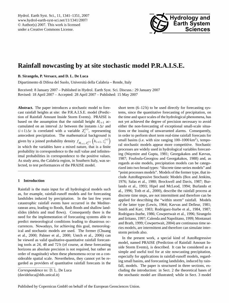
Fig. 3. (a)Mapping ofθh,z parameter;(b) Digital Elevation Modelof the Calabria region.

are rainy. In order to respect the hypothesis of stationaryprocess, only the data measured during the “rainy season”,1 October–31 May has been used (De Luca, 2005). In thisperiod, correlation structure, mean and variance of the sam-ple appear significantly homogeneous. In particular, consid-ering hourly rain measurements of Cosenza raingauge, cov-ering a period of about 15 years, and subdividing the yearinto three subperiods of four months (1 October–31 January;1 February–31 May; 1 June–30 September), sample meansand variances of the variable H are shown in Table 1, and

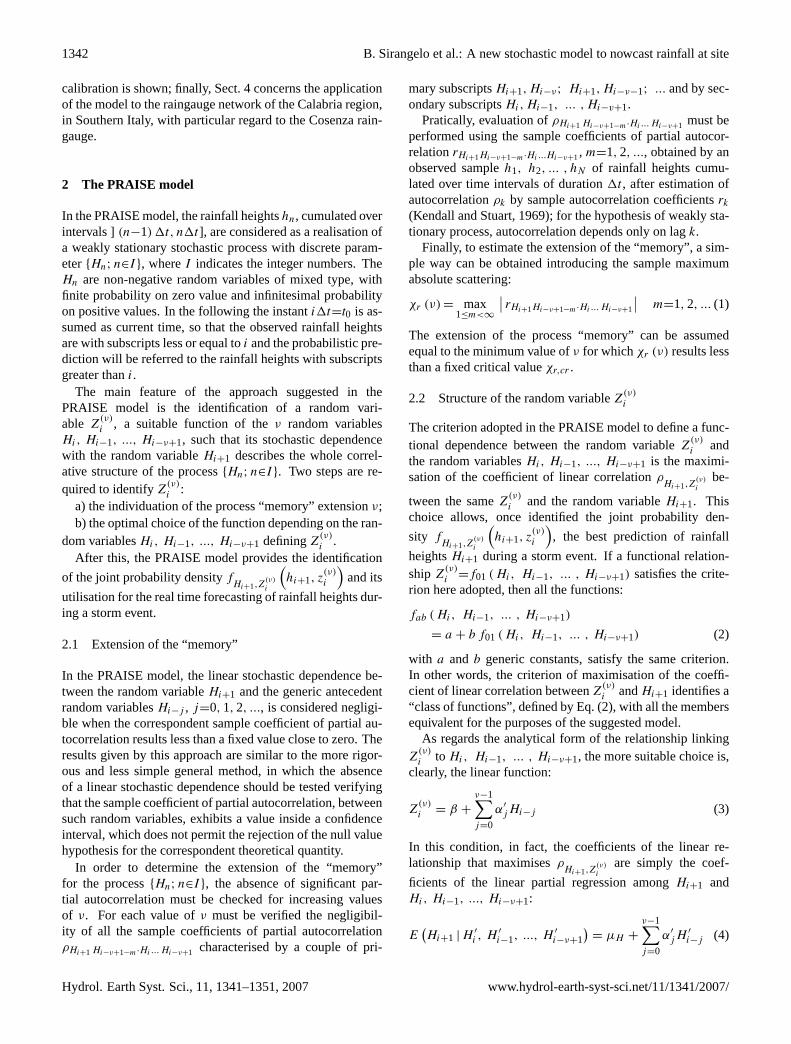
Fig. 4. Memory extension (rainy season) referred to the CosenzaRaingauge.

Table 1. Cosenza raingauge: sample means and variances for threesubperiods of the year.

Season SubPeriod samplemean(mm)

samplevariance(mm2)

Rainy season1 Oct–31 Jan 0.14 0.091

1 Feb–31 May 0.12 0.084

Dry season 1 June–30 Sep 0.04 0.026

sample autocorrelograms are reported in Fig. 2. It appearsplausible to consider as stationary the period comprising thefirst two subperiods. It must be highlighted that, because ofthe sample size, stationarity analysis based on a further sub-division into more subperiods appears unsuitable because ofthe greater uncertainty of moments evaluation.

The model parameters have been estimated for every rain-gauge. Subsequently, each parameter was mapped on thespatial regional domain by using a spline technique. The ex-tension of the “memory”, determined by the technique de-scribed in the Sect. 2.1 fixingχr,cr=0.025, has been foundequal toν=8 for all the tele-metering raingauges. An exam-ple of parameter mapping, referred toθh,z is represented inFig. 3a, that shows greater values, and consequently highervalues ofρ(+,+)

Hi+1,Z(ν)i

correlation, located in the part of region

characterized by greater altitude, as depicted by the compar-ison with the Digital Elevation Model of the Calabria region(Fig. 3b).

In Fig. 4 memory extension, referred to the rainy seasonof the Cosenza raingauge, is depicted.



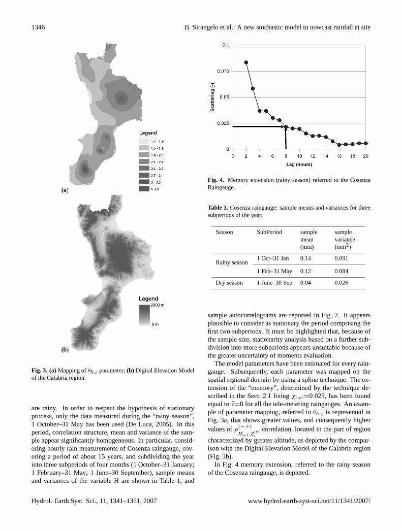
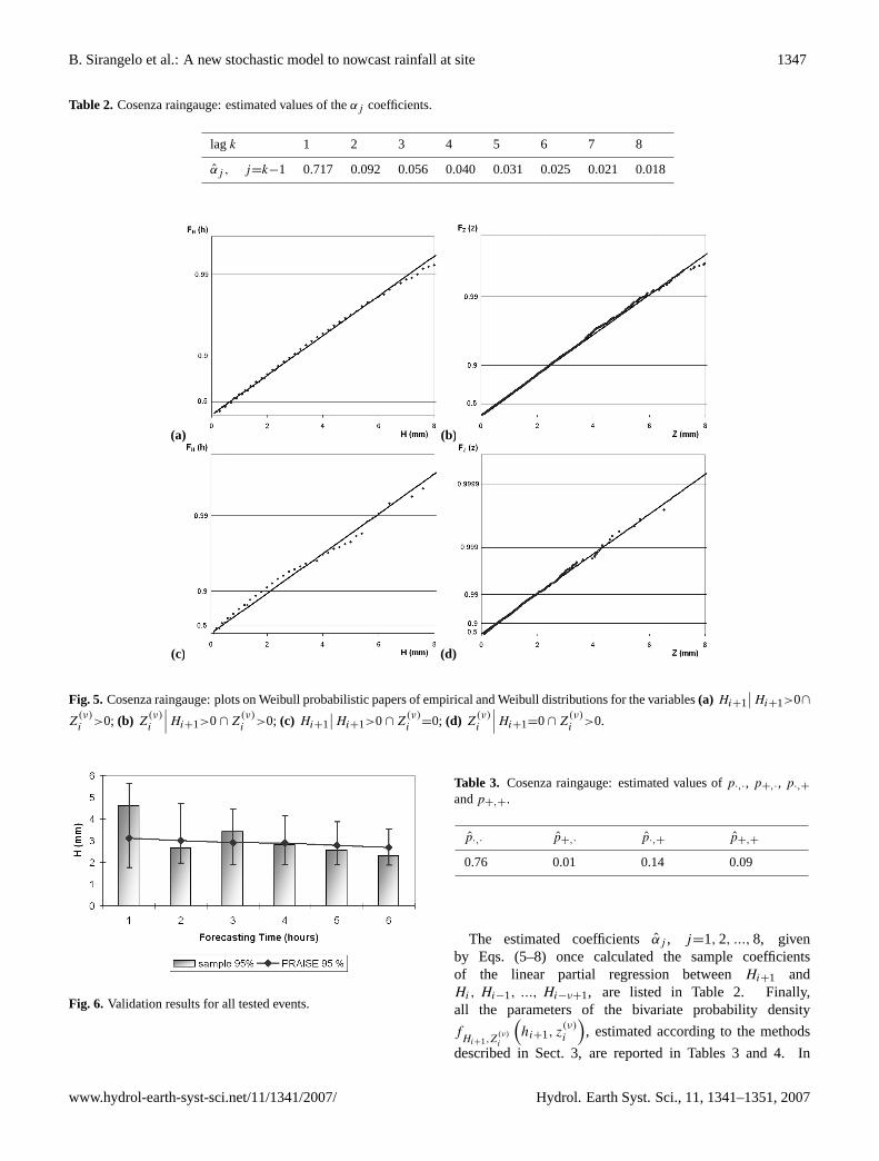
Table 2. Cosenza raingauge: estimated values of theαj coefficients.

lagk 1 2 3 4 5 6 7 8

αj , j=k−1 0.717 0.092 0.056 0.040 0.031 0.025 0.021 0.018

(a) (b)

(c) (d)

Fig. 5. Cosenza raingauge: plots on Weibull probabilistic papers of empirical and Weibull distributions for the variables(a) Hi+1∣∣Hi+1>0∩

Z(ν)i

>0; (b) Z(ν)i

∣∣∣Hi+1>0 ∩ Z(ν)i

>0; (c) Hi+1∣∣Hi+1>0 ∩ Z

(ν)i

=0; (d) Z(ν)i

∣∣∣Hi+1=0 ∩ Z(ν)i

>0.

Fig. 6. Validation results for all tested events.

Table 3. Cosenza raingauge: estimated values ofp·,·, p+,·, p·,+

andp+,+.

p·,· p+,· p·,+ p+,+

0.76 0.01 0.14 0.09

The estimated coefficientsαj , j=1, 2, ..., 8, givenby Eqs. (5–8) once calculated the sample coefficientsof the linear partial regression betweenHi+1 andHi, Hi−1, ..., Hi−ν+1, are listed in Table 2. Finally,all the parameters of the bivariate probability density

fHi+1,Z

(ν)i

(hi+1, z

(ν)i

), estimated according to the methods

described in Sect. 3, are reported in Tables 3 and 4. In



(a) (b)

(c)

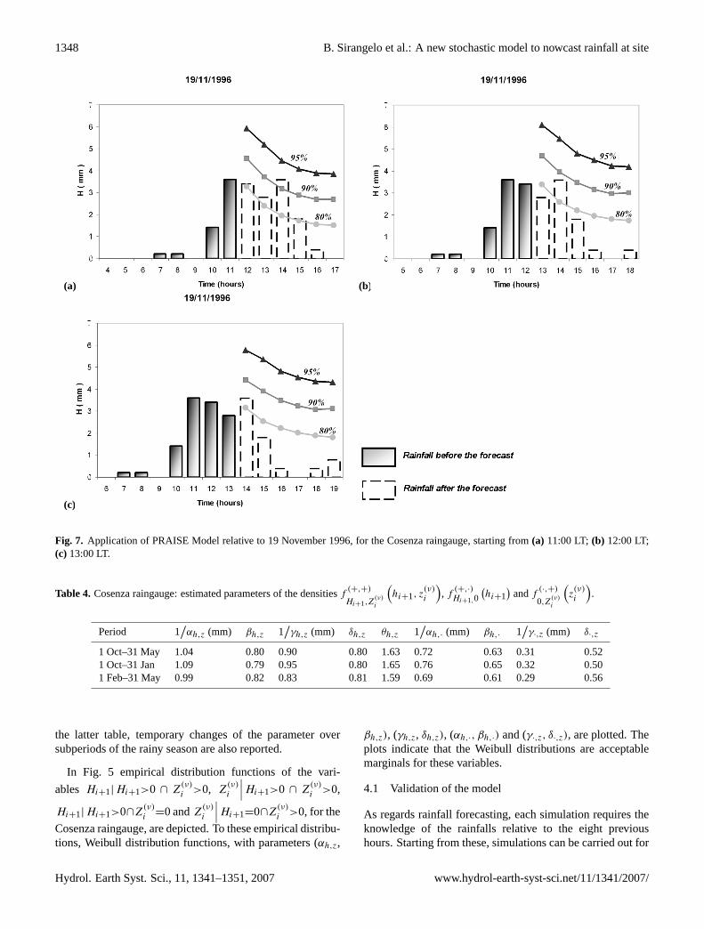
Fig. 7. Application of PRAISE Model relative to 19 November 1996, for the Cosenza raingauge, starting from(a) 11:00 LT; (b) 12:00 LT;(c) 13:00 LT.

Table 4. Cosenza raingauge: estimated parameters of the densitiesf(+,+)

Hi+1,Z(ν)i

(hi+1, z

(ν)i

), f

(+,·)Hi+1,0

(hi+1

)andf

(·,+)

0,Z(ν)i

(z(ν)i

).

Period 1/αh,z (mm) βh,z 1

/γh,z (mm) δh,z θh,z 1

/αh,· (mm) βh,· 1

/γ·,z (mm) δ·,z

1 Oct–31 May 1.04 0.80 0.90 0.80 1.63 0.72 0.63 0.31 0.521 Oct–31 Jan 1.09 0.79 0.95 0.80 1.65 0.76 0.65 0.32 0.501 Feb–31 May 0.99 0.82 0.83 0.81 1.59 0.69 0.61 0.29 0.56

the latter table, temporary changes of the parameter oversubperiods of the rainy season are also reported.

In Fig. 5 empirical distribution functions of the vari-

ables Hi+1| Hi+1>0 ∩ Z(ν)i >0, Z

(ν)i

∣∣∣Hi+1>0 ∩ Z(ν)i >0,

Hi+1| Hi+1>0∩Z(ν)i =0 andZ

(ν)i

∣∣∣Hi+1=0∩Z(ν)i >0, for the

Cosenza raingauge, are depicted. To these empirical distribu-tions, Weibull distribution functions, with parameters (αh,z,

βh,z), (γh,z, δh,z), (αh,·, βh,·) and (γ·,z, δ·,z), are plotted. Theplots indicate that the Weibull distributions are acceptablemarginals for these variables.

4.1 Validation of the model

As regards rainfall forecasting, each simulation requires theknowledge of the rainfalls relative to the eight previoushours. Starting from these, simulations can be carried out for



(a) (b)

(c)

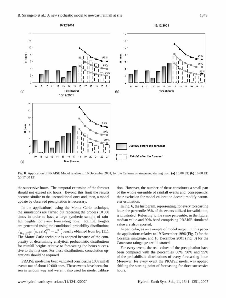
Fig. 8. Application of PRAISE Model relative to 16 December 2001, for the Catanzaro raingauge, starting from(a) 15:00 LT;(b) 16:00 LT;(c) 17:00 LT.

the successive hours. The temporal extension of the forecastshould not exceed six hours. Beyond this limit the resultsbecome similar to the unconditional ones and, then, a modelupdate by observed precipitation is necessary.

In the applications, using the Monte Carlo technique,the simulations are carried out repeating the process 10 000times in order to have a large synthetic sample of rain-fall heights for every forecasting hour. Rainfall heightsare generated using the conditional probability distributions

fHi+1| Z

(ν)i

(hi+1|Z

(ν)i = z

(ν)i

), easily obtained from Eq. (11).

The Monte Carlo technique is adopted because of the com-plexity of determining analytical probabilistic distributionsfor rainfall heights relative to forecasting the hours succes-sive to the first one. For these distributions, convolution op-erations should be required.

PRAISE model has been validated considering 100 rainfallevents out of about 10 000 ones. These events have been cho-sen in random way and weren’t also used for model calibra-

tion. However, the number of these constitutes a small partof the whole ensemble of rainfall events and, consequently,their exclusion for model calibration doesn’t modify param-eter estimation.

In Fig. 6, the histogram, representing, for every forecastinghour, the percentile 95% of the events utilized for validation,is illustrated. Referring to the same percentile, in the figure,median value and 90% band comprising PRAISE simulatedvalue are also reported.

In particular, as an example of model output, in this paperthe applications relative to 19 November 1996 (Fig. 7) for theCosenza raingauge, and 16 December 2001 (Fig. 8) for theCatanzaro raingauge are illustrated.

For every event, the real values of the precipitation havebeen compared with the percentiles 80%, 90% and 95%of the probabilistic distributions of every forecasting hour.Moreover, for every event the PRAISE model was appliedshifting the starting point of forecasting for three successivehours.



The Figs. 7–8 show that rainfall heights of the real eventfall between percentiles 80% and 90%. These results indi-cate the capability of the model to identify, for the forecasthours, statistical confidence limits containing the real rainfallheights.

5 Conclusions

This paper presents a new stochastic model named PRAISEto forecast rainfall heights at site. The mathematical back-ground is characterized by a bivariate probability distribu-tion, referred to the random variablesHi+1 andZ

(ν)i , repre-

senting rainfall in a generic site and antecedent precipitationin the same site.

The peculiarity of PRAISE is the availability of the prob-abilistic distributions of rainfall heights for the forecastinghours, conditioned by the values of observed precipitation.

PRAISE was applied to all the telemetering raingauges ofthe Calabria region, in Southern Italy; the calibration modelshows that the hourly rainfall series present a constant valueof memoryν equal to 8 h, for every raingauge of the Calabrianetwork. Moreover, analysingθh,z parameter mapping, itmust be pointed out how higher values ofρ

(+,+)

Hi+1,Z(ν)i

correla-

tion are located in the part of region characterized by greateraltitude.

The examples of validation, presented here, regarding theCosenza and Catanzaro raingauges, indicate the capabilityof the model to identify, for the forecasting hours, statisticalconfidence limits containing the real rainfall heights. ThePRAISE model therefore can be considered a very useful andsimple tool for forecasting precipitation and consequently,using rainfall-runoff models or hydro-geotechnical models,floods or landslides, in planning and managing a warningsystem.

Edited by: A. Gelfan

References

Abramowitz, M. and Stegun, I. A.: Handbook of mathematicalfunctions, Dover, New York, NY, 1970.

Box, G. E. P. and Jenkins, G. M.: Time series analysis: forecastingand control, Holden-Day, S.Francisco, 1976.

Brockwell, P. J. and Davis, R. A.: Time Series. Theory and Meth-ods, Springer Verlag, New York, NY, 1987.

Burlando, P., Rosso, R., Cadavid, L. G., and Salas, J. D.: Forecast-ing of short-term rainfall using ARMA models, J. Hydrol., 144,193–211, 1993.

Burlando, P., Montanari, A., and Ranzi, R.: Forecasting of stormrainfall by combined use of radar, rain gages and linear models,Atmos. Res., 42, 199–216, 1996.

Calenda, G. and Napolitano, F.: Parameter estimation of Neyman-Scott processes for temporal point rainfall simulation, J. Hydrol.,225, 45–66, 1999.

Chuang, Hui-Ya, and Sousounis, P. J.: A technique for generat-ing idealized initial and boundary conditions for the PSU-NCARModel MM5, Mon. Wea. Rev., 128, 2875–2882, 2000.

Cowpertwait, P. S. P., O’Connell, P. E., Metcalfe, A. V., and Mawds-ley, J. A.: Stochastic point process modelling of rainfall. I. Singlesite fitting and validation, J. Hydrol., 175, 17–46, 1996.

Cowpertwait, P. S. P.: Mixed rectangular pulses models of rainfall,Hydrol. Earth Syst. Sci., 8, 993–1000, 2004,http://www.hydrol-earth-syst-sci.net/8/993/2004/.

De Luca, D. L.: Metodi di previsione dei campi di pioggia. Tesi diDottorato di Ricerca, Universita della Calabria, Italy, 2005.

Foufoula-Georgiou, E. and Georgakakos, K. P.: Recent advances inspace-time precipitation modelling and forecasting, Recent Ad-vances in the Modelling of Hydrologic Systems, NATO ASI Ser.,1988.

Georgakakos, K. P. and Kavvas, M. L.: Precipitation analysis, mod-eling and prediction in hydrology, Rev. Geophys., 25(2), 163–178, 1987.

Hipel, K. W. and McLeod, A. I.: Time series Modeling of WaterResources and Environmental Systems, Elsevier Science, 1994.

Kavvas, M. L. and Delleur, J. W.: A stochastic cluster model ofdaily rainfall sequences, Water Resour. Res., 17(4), 1151–1160,1981.

Kendall, M. G. and Stuart, A.: The advanced Theory of Statistics,Griffin, London, 1969.

Kotz, S., Balakrishanan, N., and Johnson, N. L.: Continuous Mul-tivariate Distributions – Models And Applications, Wiley, NewYork, NY, 2000.

Lewis, P. A. W.: Stochastic Point Processes, Wiley, New York, NY,1964.

Montanari, A. and Brath, A.: Maximum likelihood estimation forthe seasonal Neyman-Scott rectangular pulses model for rainfall,Proc. of the EGS Plinius Conference, 297–309, Maratea, Italy,1999.

Palmer, T. N., Brankovic, C., Buizza, R., Chessa, P., Ferranti, L.,Hoskins, B. J., and Simmons, A. J.: A review of predictabilityand ECMWF forecast performance, with emphasis on Europe,ECMWF Research Department Technical Memorandum n. 326,ECMWF, Shinfield Park, Reading RG2-9AX, UK, 2000.

Press, W. H., Flannery, B. P., Teukolsky, S. A., and Vetterling, W. T.:Numerical Recipes in C. The art of scientific computing, Cam-brige University Press, 1988.

Rodriguez-Iturbe, I., Gupta, V. K., and Waymire, E.: Scale con-sideration in modelling of temporal rainfall, Water Resour. Res.,20(11), 1611–1619, 1984.

Rodriguez-Iturbe, I.: Scale of fluctuation of rainfall models, WaterResour. Res., 22(9), 15S–37S, 1986.

Rodriguez-Iturbe, I., Cox, D. R., and Isham, V.: Some models forrainfall based on stochastic point processes, Proc. Royal Soc.London, A, 410, 269–288, 1987.

Salas, J. D., Delleur, J. W., Yevjevich, V., and Lane, W. L.: Appliedmodelling of hydrologic time series, Water Resources Publica-tions, Littleton, CO, 1980.

Sirangelo, B. and Iiritano, G.: Some aspects of the rainfall analysisthrough stochastic models, Excerpta, 11, 223–258, 1997.

Smith, J. A. and Karr, A. F.: A point process model of summerseason rainfall occurrences, Water Resour. Res., 19(1), 95–103,1983.

Toth, E., Brath, A., and Montanari, A.: Comparison of short-term


http://www.hydrol-earth-syst-sci.net/8/993/2004/


rainfall prediction models for real-time flood forecasting, J. Hy-drol., 239(1), 132–147, 2000.

Untch, A., Miller, M., Hortal, M., Buizza, R., and Janssen, P.: To-wards a global meso-scale model: the high-resolution systemTL799L91 & TL399L62 EPS, Newsletter n. 108, ECMWF, Shin-field Park, Reading RG2-9A, UK, 2006.

Waymire, E. and Gupta, V. K.: The mathematical structure of rain-fall representations, 1. A review of the stochastic rainfall models,Water Resour. Res., 17(5), 1261–1272, 1981.


rainfall nowcasting by at site stochastic model p.r.a.i.s.e

Documents