THRESHOLD MODELS FOR RAINFALL AND CONVECTION:

DETERMINISTIC VERSUS STOCHASTIC TRIGGERS ∗

SCOTT HOTTOVY†, SAMUEL N. STECHMANN†‡

Abstract. This paper investigates stochastic models whose dynamics switch depending on thestate/regime of the system. Such models have been called “hybrid switching diffusions” and exhibit“sliding dynamics” with noise. Here the aim is an application to models of rainfall, convection, andwater vapor, where two states/regimes are considered: precipitation and non-precipitation. Regimechanges are modeled with a “trigger function,” and four trigger models are considered: deterministictriggers (i.e. Heaviside function) or stochastic triggers (finite-state Markov jump process), with eithera single threshold for regime transitions or two distinct thresholds (allowing for hysteresis). Thesetriggers are idealizations of those used in convective parameterizations of global climate models, andthey are investigated here in a model for a single atmospheric column. Two types of results arepresented here. First, exact statistics are presented for all four models, and a comparison indicateshow the trigger choice influences rainfall statistics. For example, it is shown that the average rainfallis identical for all four triggers, whereas extreme rainfall events are more likely with the stochastictrigger. Second, the stochastic triggers are shown to converge to the deterministic triggers in the limitof fast transition rates. The convergence is shown using formal asymptotics on the Master-Fokker-Planck equations, where the limit is an interesting Fokker-Planck system with Dirac delta couplingterms. Furthermore, the convergence is proved in the mean-square sense for pathwise solutions.

Key words. Moist atmospheric convection, Sliding Dynamics, Hybrid Switching Diffusions,Convective Parameterization

AMS subject classifications. 00A69, 60J70, 86A10

1. Introduction. This paper is related to stochastic models that exhibit slidingdynamics with noise [29, 28] and hybrid switching diffusions [36]. In particular here,these types of stochastic models arise in the context of an atmospheric science problem:What is the best way to model the onset and demise of atmospheric convection and/orrainfall?

The mathematical form of the model is

dq = Sσ dt+Dσ dW, (1.1)

where q ∈ R is a scalar. The drift Sσ and diffusion Dσ coefficients are constantand have a form that switches when the discrete process σt switches its value. Forsimplicity, σt will be a two-state process that takes the value 0 or 1. Furthermore, thedynamics of σt will take one of two forms. In one case, the value of σt switches whenqt reaches a fixed threshold (which will be labeled qc or qnp),–i.e., σt = H(qt − qc).We refer to this type of trigger as a “deterministic trigger.” This is similar to thesliding dynamics with noise discussed in [29, 28], except here the diffusion Dσ is state-dependent, and two thresholds, qc and qnp, are used in a way that allows hysteresis.In the second case, σt is a Markov jump process whose transition rates depend on qt.Specifically, the transition rates have a form that allows a transition to occur when qtcrosses the fixed threshold qc, but the transition occurs stochastically at some randomvalue of q > qc. We call this a “stochastic trigger.” The two different types of triggerswith one or two thresholds gives four different models. We call the models with astochastic trigger with one or two thresholds S1 and S2, respectively. Similarly, themodels with a deterministic trigger are referred to as D1 and D2. See Figure 1.1

1

Time [hrs]

Moi

stur

e [m

m]

Example of the (S1) process

Switch to wet stateat random time

Switch to dry stateat random time

qc

Time [hrs]

Moi

stur

e [m

m]

Example of the (D1) process

In dry state

In wet state

↓

Switch to dry

↑Switch to wet

qc

Time [hrs]

Moi

stur

e [m

m]

Example of the (S2) process

Switch to wet stateat random time

Switch to dry stateat random time

No change in dynamics

qnp

qc

Time [hrs]

Moi

stur

e [m

m]

Example of the (D2) process

In wet state

In dry state

No change in dynamics

↓Switch to dry

↑Switch to wet

qnp

qc

Fig. 1.1. An example of the four different models used in this study. For all models, theswitch to the wet state (grey line) occurs when the threshold qc is reached from below. For the 1threshold models (left), the switch to the dry state (black line) occurs when the threshold qc is reachedfrom above. For the 2 threshold models (right), on the other hand, the switch to dry state occurswhen a different threshold qnp is reached from above. These switches occur deterministically (top,D) or stochastically (bottom, S). For the deterministic trigger models (top panels), the switch fromone state to the other occurs immediately when the threshold is reached. For the stochastic triggermodels (bottom panels), on the other hand, the switch from one state to the other does not occurimmediately when the threshold is reached; instead, there is a stochastic delay in the switching, andthe switching occurs at a random value of q beyond the threshold.

for sample trajectories of each model. In this way, the “stochastic trigger” σt processshould converge to the “deterministic trigger” σt process as the transition rate λ tendsto infinity. One of the main objectives of this paper is to investigate this convergenceand to explore the statistics of qt and σt in each of the two cases.

From an atmospheric science point of view, these are idealized stochastic modelsfor rainfall. The variable qt represents the amount of water vapor in an atmosphericcolumn, which extends vertically above an area of roughly 10 km × 10 km—perhapseven 100 km × 100 km. Within such an atmospheric column, clouds and rainfall willoccasionally develop, and the development can occur so rapidly that it appears to be“triggered.” To describe the trigger mathematically, one simple approach is to use anindicator function σt that equals 1 when the column is raining and 0 when there isno rain.

The problem of modeling the trigger σt is important for both general circulationmodels [2, 16, 33] and for hydrological models of rainfall [3, 10, 26, 5, 27, 1]. TheD1 model is an idealization of parameterizations of convection in general circulationsmodels and idealized atmospheric models [2, 22, 17, 8, 30]. In the models consideredhere, two thresholds (qc and qnp) will be used [32] instead of the single threshold qc,

†Department of Mathematics, University of Wisconsin–Madison‡Department of Atmospheric and Oceanic Sciences, University of Wisconsin–Madison∗The research of S.N.S. is partially supported by the ONR Young Investigator Program through

grant ONR N00014- 12-1-074, and S.H. is supported as a postdoctoral research associate on thisgrant.

2

and the two cases will be compared and contrasted. The motivation for introducing asecond threshold qnp comes from Figure 6 of [21]; this figure shows that more than halfof all rainfall occurs below qc; hence it may be most realistic to use a second thresholdqnp for the shutdown of rainfall. Stochastic trigger models with smoothed versionsof Heaviside functions have been studied previously [18, 19, 31]. This alternative isperhaps more realistic than the use of a Heaviside function, since there is likely nounique, fixed threshold value qc that demarcates the transition from raining to non-raining for every rain event; nevertheless, the simplicity of the Heaviside function isappealing.

The motivation for the present investigation is threefold.

First, in general circulation models of the atmosphere, the trigger is a key elementof the convective parameterization, and it can have significant effects on the realismof tropical convection, convectively coupled waves, and the Madden–Julian Oscilla-tion [16, 14]. While “deterministic triggers” are traditionally used [2, 22, 17, 8, 30],“stochastic triggers” have been proposed and advanced to improve the simulated vari-ability of tropical convection and waves [18, 13, 19, 12, 7]. The models of the presentpaper can be thought of as idealized versions of realistic stochastic triggers. As such,their value is that they offer exactly solvable statistics for ease of comparison of thetwo types of triggers; and they allow for proofs of convergence with the rate of conver-gence with respect to the transition rate. This also provides mathematically rigorousguidance for how the two types of triggers are different.

Second, this paper provides a better understanding of models for a new perspec-tive on precipitation and water vapor observations [24, 21, 23]. The observed statis-tics have shown a similarity with critical phenomena and other statistical physicsparadigms. To better understand the physical processes underlying these statistics,Stechmann and Neelin [31] designed and analyzed a model of the form (1.1), and theyshowed that the model reproduces many of the observed statistics. Subsequently,Stechmann and Neelin [32] introduced a simpler version of the model that uses deter-ministic triggers instead of stochastic triggers. The model with deterministic triggersis advantageous because its exact statistics are easily accessible; however, this sim-plification comes at the expense of slightly less realistic statistics. Hence, for futurestudies, an important question is: how closely related are the models with determin-istic and stochastic triggers? Can the approximation error be quantified? Also alongthese lines, exact statistics are presented here for a case with stochastic triggers; thiscase involves a simpler parameter regime than in [31], and some of the formulas canbe prohibitively complex compared to the deterministic-trigger model of [32].

Third, the model is an example of hybrid switching diffusions and random dy-namical systems with sliding dynamics not studied before. The models, S1 and S2,are examples of switching diffusion systems with discontinuous transition functionsdefined in equation (2.2), which differs from the examples in [36]. The D1 and D2models are examples of dynamical systems that undergo sliding dynamics with state–dependent noise. Furthermore, the D2 model has a manifold qnp ≤ q ≤ qc where thedynamics of the system depend on the state of σt. That is, the state of σt can not bederived from the moisture value of qnp ≤ qt ≤ qc alone.

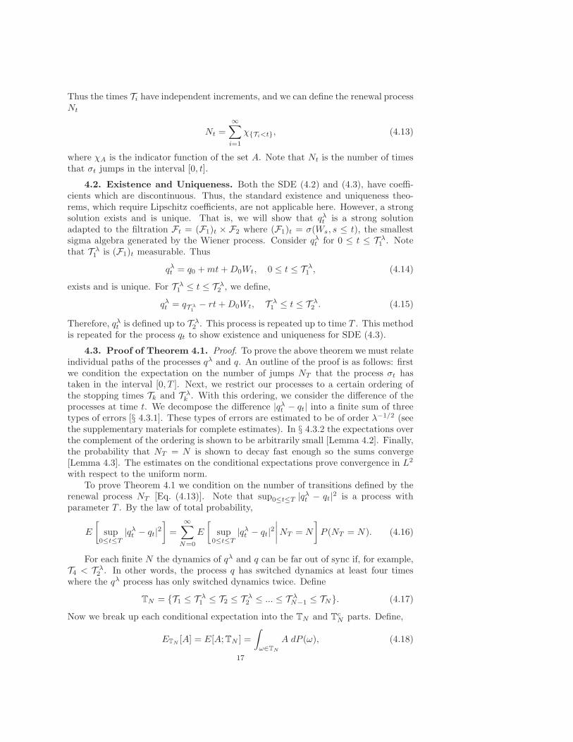
In this paper, we prove that the hybrid switching diffusion model S2 convergesto deterministic trigger model D2 as the transition rate tends to infinity. To do so,we use the Fokker-Planck equation to derive the first and second moments of thejumping time, i.e. the time it takes the λ–process to jump once it reaches the criticalthreshold. The first and second moments are of order λ−1/2 which ultimately controls

3

the L2 convergence.The models here are mathematically tractable idealizations of the atmosphere,

and they neglect or simplify many aspects of atmospheric physics and dynamics. Amore complete description would require other variables besides just water vapor (e.g.,temperature) and would require knowledge of the water vapor q(z, t) at each height zabove the Earth’s surface z = 0, rather than just the column-averaged water vapor qtthat is considered here. Also, a more complete description would partition rainfall intostratiform and deep convective components [12, 7, 11, 20]. Despite the simplicity ofthe models here, they contain the important ingredients of thresholds and stochasticforcing which are mainstays in both complex and idealized models alike.

The outline of the paper is as follows: In § 2, we give a more detailed explanationof the models S1,S2,D1, and D2. In § 3 we study numerous properties of the model.First we derive the Fokker–Planck equation for D2 using an asymptotic expansion ofthe S2 Fokker-Planck equation [§ 3.2]. Then we find the exact stationary solutionsfor the four models [§ 3.3], and use them to study conditional and marginal statistics[§ 3.4]. We compare the mean event sizes for S2 and D2 in § 3.5. In § 4, we provethe main theorem of the paper [Theorem 4.1], that the S2 process converges, in L2,to the D2 process as λ tends to infinity.

2. Model Description. In this section we introduce a simple stochastic equa-tion to model water vapor for a single atmospheric column. The column water vaporat time t, denoted qt is defined by the stochastic different equation (SDE),

dqλt =

mdt+D0dWt σλt = 0

−rdt+D1dWt σλt = 1,

(2.1)

with m > 0 for moistening and r > 0 for rain rates, D1 > D0 > 0 are the noisecoefficients, and the initial condition qλ0 = q0, σ

λ0 = 0. The dynamics of σλ

t ∈ 0, 1are as follows: when σλ

t = 0 the probability that σλ transitions to 1 is governedby an exponential random variable with the transition rate r01(qt). Similarly, whenσλt = 1 the transition rate is r10(qt). That is, when σt = 0, the probability that the

process transitions to the rain state after a short amount of time, σt+∆t = 1, is givenapproximately by r01(qt)∆t, and similarly for the transition from 1 to 0. The valuesq = qc and q = qnp = qc − qǫ, for qǫ relatively small compared to qc, play a criticalrole in the transition to and from convection.

There are many possible physically realistic choices for the rate function rij(q).For example, in [31] the rate function is a hyperbolic tangent function. Another choicewould be to set r01(q) = 0 for q < qc and r01(q) = 1 once q = qc. Thus, the processswitches dynamics after an exponential random time. SDE, in which a smooth ratefunction for the switching process is used, are studied in [36]. In this paper, we usethe rate functions

r01(q) = λH(q − qc)r10(q) = λH(qnp − q).

(2.2)

The above rate function is studied in this paper because exact formulas are derived,such as the stationary density [Sec. 3.3] and the jumping time distribution — i.e.when qt = qc or qnp, the time it takes to switch dynamics.

The solution qt of SDE (2.1) is a Brownian motion with positive (σ = 0) ornegative (σ = 1) drift. Once the process switches dynamics, the process is still aBrownian motion with drift. Thus, (qt, σt) is a Markov process, and despite thediscontinuity of the coefficients of SDE (2.1) there exists a unique solution (see § 4).

4

We call the above model, the stochastic model with two thresholds (qc and qnp)or S2. Three other models that are closely related to the above are considered in thispaper, S1, D1, and D2. The stochastic model with one threshold (qc), called S1, isinterpreted as the above model with qnp = qc − qǫ → qc as qǫ → 0. The transitionrates for these two models are diagrammed in Figure 2.1. The two deterministicmodels, with one threshold and two (D1 and D2) are interpreted in the same way asthe stochastic, except that the process σ switches dynamics immediately when hittingthe threshold. This can be interpreted as having an infinite transition rate.

Moisture q [mm]

r 01(q

) [h

r−1 ]

Transition Rates for S1

qc

0

λa)

Moisture q [mm]

r 10(q

) [h

r−1 ]

qc

0

λb)

Moisture q [mm]

r 01(q

) [h

r−1 ]

Transition Rates for S2

qnp

qc

0

λc)

Moisture q [mm]

r 10(q

) [h

r−1 ]

qnp

qc

0

λd)

Fig. 2.1. The transition rates for the S1 and S2 models are shown above. The one thresholdmodel S1 is plotted on the left. The two threshold model S2 is plotted on the right.

Later in the paper [§ 4], these models are shown to be approximations to one an-other when a certain limit is taken. I.e. the one threshold models are approximationsto the corresponding two threshold models for qǫ ≪ 1, and the deterministic modelsare approximations to the stochastic models for λ ≫ 1. The convergence is mappedout in Figure 2.2, and is discussed in Section 4. Note that the jumping time usedin this paper is longer than an exponential random time as soon as the threshold isreached and the hyperbolic tangent rate function used in [31]. Thus proving that theabove model converges to D2, implies many other models (e.g. the model in [31])converge as well.

Fig. 2.2. A figure describing the convergence of the separate models. The arrows “→” implyconvergence in L2, and “⇒” are weak convergence (or in distribution), see § 4.

5

3. Properties of the Models. In this section, we derive the Fokker-Planckequations for the models D1 and D2. This includes giving a heuristic derivationof the Fokker-Planck equation for D2 [§ 3.2] in the limit as λ → ∞. With theseequations we solve for exact statistics of the models. The statistics that we studyhere, for the four different models, are the stationary probability density function[§ 3.3], conditioned statistics computed from the stationary density [§ 3.4], and theevent duration [§ 3.5]. These statistics are exactly solvable for the four models.

3.1. The Fokker-Planck Equation for S2. To study the stationary densityof the models described in § 2, we use the Fokker-Planck (or Kolmogorov forward)equation for the SDE of the corresponding model. The addition of a continuous timediscrete valued process σt adds another term to the classic Fokker-Planck equation.For example, consider the process (qt, σt) governed by SDE (2.1) with the S2 type oftrigger. Then σ has a q-dependent generator, such that for a suitable function φ(q),

Q(q)φ(q) =

(

−λH(q − qc) λH(q − qc)λH(qnp − q) −λH(qnp − q)

)(

φ0(q)φ1(q)

)

. (3.1)

Given the SDE for the process qt, the joint generator for (q, σ) is

L(q,σ)f(q) =

(

L0f0(q) 00 L1f1(q)

)

+Q(q)f(q), (3.2)

where Li is the generator of SDE (2.1) with σ = i, i = 0, 1 [9, 36]. The Fokker-Planck equation is the adjoint of the generator L(q,σ) above. It is a coupled PDE withsolutions ρ0(q, t), ρ1(q, t). In a slight abuse of terminology, we refer to these solutionsas “densities” of the dry (ρ0) and wet (ρ1) states, respectively. However, ρ0 and ρ1do not integrate to one. They arise naturally from the joint density, ρ(q, σ, t), bypartitioning the density into σ = 0 and σ = 1, i.e.

ρ(q, σ, t) = δσ0ρ(q, 0, t) + δσ1ρ(q, 1, t) = ρ0(q, t) + ρ1(q, t). (3.3)

In the case for S2 the Fokker-Planck equation is

∂

∂t

(

ρ0(q, t)ρ1(q, t)

)

=− ∂

∂q

(

m 00 −r

)(

ρ0(q, t)ρ1(q, t)

)

+1

2

∂2

∂q2

(

D20 00 D2

1

)(

ρ0(q, t)ρ1(q, t)

)

(3.4)

+λ

(

−H(q − qc) H(qnp − q)H(q − qc) −H(qnp − q)

)(

ρ0(q, t)ρ1(q, t)

)

.

The total probability of the system is conserved, where the state of the system ischaracterized by the column water vapor q ∈ R and the precipitation indicator σ ∈0, 1. Thus we have the condition

1∑

σ=0

∫ ∞

−∞

ρ(q, σ, t) dq =

∫ ∞

−∞

ρ0(q, t) + ρ1(q, t) dq = 1, (3.5)

for all t ∈ [0,∞).

The Fokker-Planck equation for S1 can easily be recovered from the formula aboveby taking qnp = qc.

6

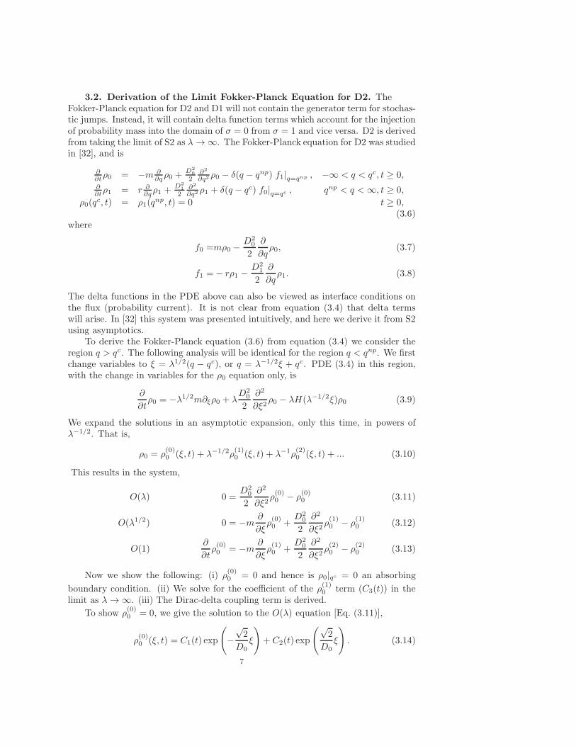
3.2. Derivation of the Limit Fokker-Planck Equation for D2. TheFokker-Planck equation for D2 and D1 will not contain the generator term for stochas-tic jumps. Instead, it will contain delta function terms which account for the injectionof probability mass into the domain of σ = 0 from σ = 1 and vice versa. D2 is derivedfrom taking the limit of S2 as λ → ∞. The Fokker-Planck equation for D2 was studiedin [32], and is

∂∂tρ0 = −m ∂

∂qρ0 +D2

0

2∂2

∂q2 ρ0 − δ(q − qnp) f1|q=qnp , −∞ < q < qc, t ≥ 0,∂∂tρ1 = r ∂

∂qρ1 +D2

1

2∂2

∂q2 ρ1 + δ(q − qc) f0|q=qc , qnp < q < ∞, t ≥ 0,

ρ0(qc, t) = ρ1(q

np, t) = 0 t ≥ 0,(3.6)

where

f0 =mρ0 −D2

0

2

∂

∂qρ0, (3.7)

f1 =− rρ1 −D2

1

2

∂

∂qρ1. (3.8)

The delta functions in the PDE above can also be viewed as interface conditions onthe flux (probability current). It is not clear from equation (3.4) that delta termswill arise. In [32] this system was presented intuitively, and here we derive it from S2using asymptotics.

To derive the Fokker-Planck equation (3.6) from equation (3.4) we consider theregion q > qc. The following analysis will be identical for the region q < qnp. We firstchange variables to ξ = λ1/2(q − qc), or q = λ−1/2ξ + qc. PDE (3.4) in this region,with the change in variables for the ρ0 equation only, is

∂

∂tρ0 = −λ1/2m∂ξρ0 + λ

D20

2

∂2

∂ξ2ρ0 − λH(λ−1/2ξ)ρ0 (3.9)

We expand the solutions in an asymptotic expansion, only this time, in powers ofλ−1/2. That is,

ρ0 = ρ(0)0 (ξ, t) + λ−1/2ρ

(1)0 (ξ, t) + λ−1ρ

(2)0 (ξ, t) + ... (3.10)

This results in the system,

O(λ) 0 =D2

0

2

∂2

∂ξ2ρ(0)0 − ρ

(0)0 (3.11)

O(λ1/2) 0 = −m∂

∂ξρ(0)0 +

D20

2

∂2

∂ξ2ρ(1)0 − ρ

(1)0 (3.12)

O(1)∂

∂tρ(0)0 = −m

∂

∂ξρ(1)0 +

D20

2

∂2

∂ξ2ρ(2)0 − ρ

(2)0 (3.13)

Now we show the following: (i) ρ(0)0 = 0 and hence is ρ0|qc = 0 an absorbing

boundary condition. (ii) We solve for the coefficient of the ρ(1)0 term (C3(t)) in the

limit as λ → ∞. (iii) The Dirac-delta coupling term is derived.

To show ρ(0)0 = 0, we give the solution to the O(λ) equation [Eq. (3.11)],

ρ(0)0 (ξ, t) = C1(t) exp

(

−√2

D0ξ

)

+ C2(t) exp

(√2

D0ξ

)

. (3.14)

7

The solution ρ(0)0 is assumed to be a density and hence integrable on (qc,∞), thus

C2(t) = 0. Furthermore we assume ρ0(q, t) and ∂∂qρ0(q, t) are continuous on R and

the limit as λ → ∞ must exist everywhere. Note that,

limλ→∞

∂

∂qρ0(q, t)|q=qc = lim

λ→∞−C1(t)λ

1/2

√2

D0+

∂

∂ξρ(1)0 (ξ, t)

∣

∣

∣

∣

ξ=0

+ ... (3.15)

which does not exist. Thus C1(t) = 0 and ρ(0)0 = 0. The solution to the order λ1/2

equation [Eq. (3.12)] with the integrability condition is

ρ(1)0 = C3(t) exp

(

−√2

D0ξ

)

. (3.16)

By continuity of the probability density,

ρ0((qc)−, t) = λ−1/2ρ

(1)0 (0+, t) + ... (3.17)

Because the right hand side of the above equation decays in λ then for the limit asλ → ∞, ρ0(q

c, t) → 0 for all t ≥ 0, which implies the absorbing boundary conditionfor PDE (3.6). By continuity of the derivative at qc,

∂

∂qρ0((q

c)−, t) =∂

∂ξρ(1)0 (0+, t) + λ−1ρ

(2)0 (0+, t) + ... (3.18)

=− C3(t)

√2

D0+ ... (3.19)

In the limit as λ → ∞, the above equation, when multiplied by the appropriateconstant, is a balance of fluxes at qc. Therefore,

C3(t) =

√2

D0f0

∣

∣

∣

∣

∣

qc

, (3.20)

where the flux f0 is defined as

f0(q, t) = −mρ0(q, t)−D2

0

2

∂

∂qρ0(q, t). (3.21)

Next we show the λρ0 ≈ λ1/2ρ(1)0 term converges to a delta function in the sense

of distributions. Let φ(q) be a test function on R. Recall the definition of ξ, thus wehave

∫ ∞

0

C3(t) exp

(

−√2

D0ξ

)

φ(ξλ−1/2 + qc) dξ (3.22)

=

∫ ∞

qcλ1/2C3(t) exp

(

−λ1/2

√2

D0(q − qc)

)

φ(q) dq.

Integration by parts yields,∫ ∞

qcλ1/2C3(t) exp

(

−λ1/2

√2

D0(q − qc)

)

φ(q) dq = −φ(qc)D0√2C3(t) (3.23)

+

∫ ∞

qcC3(t)

D0√2φ′(q) exp

(

−λ−1/2D0√2(q − qc)

)

dq

→C3(t)D0√2φ(qc), (3.24)

8

as λ → ∞. Thus, using equation (3.20) for C3(t),

λH(q − qc)ρ0 ≈ λ1/2ρ(1)0 → δ(q − qc)f0|q=qc , as λ → ∞. (3.25)

Along with a similar argument for the interval −∞ ≤ q ≤ qnp, we recover equa-tion (3.6) in a limit of equation (3.4) as λ → ∞.

3.2.1. Deriving the D1 Fokker-Planck equation from D2. Given equa-tion (3.6) for D2, we derive the Fokker-Planck equation for D1. To do so, we takeqnp = qc − qǫ and take the limit as qǫ → 0. The non-trivial part of this limit lies withthe interface conditions imposed by the delta functions. That is, if we integrate eachequation over their respective domains, we get the single condition,

f0(qc) = f1(q

np). (3.26)

Because of the absorbing boundary conditions, equation (3.26) is written in terms ofρ0 and ρ1 as

D20

2

∂

∂qρ0(q

c) =D2

1

2

∂

∂qρ1(q

np). (3.27)

In the limit as qǫ → 0, the above equation is a condition that must be satisfied. Thus,the Fokker-Planck equation for D1 is

∂∂tρ0 = −m ∂

∂qρ0 +D2

0

2∂2

∂q2 ρ0, q < qc

∂∂tρ1 = r ∂

∂qρ1 +D2

1

2∂2

∂q2 ρ1, q > qc

D20

2∂∂qρ0(q

c) =D2

1

2∂∂qρ1(q

c)

1 =∫∞

−∞ρ0(q, t) + ρ1(q, t) dq

(3.28)

The above system does not require ρ = ρ0+ρ1 to be continuous. In fact, for D0 6= D1,ρ is discontinuous at q = qc. This is seen in the stationary density of D1 [Eq. (3.39)].

3.3. Stationary Density. In this section we compute the stationary densitiesfor the four models using the stationary Fokker-Planck equations. We begin by findingthe stationary densities for the S2 model, denoted ρλ0 (q), ρ

λ1 (q) respectively. For S2

the stationary Fokker-Planck equation is

(

00

)

=− ∂

∂q

(

m 00 −r

)(

ρλ0 (q)ρλ1 (q)

)

+1

2

∂2

∂q2

(

D20 00 D2

1

)(

ρλ0 (q)ρλ1 (q)

)

(3.29)

+λ

(

−H(q − qc) H(qnp − q)H(q − qc) −H(qnp − q)

)(

ρλ0 (q)ρλ1 (q)

)

. (3.30)

The above equation is solved by considering the solution on the intervals

(−∞, qnp], [qnp, qc], [qc,∞) separately, then using continuity of ρ0, ρ1 and their deriva-tives.

For the stationary density of S2 define,

rλ =−r +

√

r2 + 2D21λ

D21

, and mλ =m−

√

m2 + 2D20λ

D20

. (3.31)

9

The stationary density on the different intervals is,

ρ1(q) =2rm

(m+ r)(

qǫ + mλ−rλ

rλmλ

)

(2r +D21r

λ)er

λ(q−qnp), q < qnp,

(3.32)

ρ1(q) =

m

1− e− 2r(q−qnp)

D21

(r +m)(

qǫ + mλ−rλ

rλmλ

) +r2me

2r(q−qnp)

D21

λ(m+ r)(

qǫ + mλ−rλ

rλmλ

)

D21

, qnp ≤ q ≤ qc,

(3.33)

ρ1(q) =rmem

λ(q−qc)

(m+ r)(2r +D21m

λ)(

qǫ + mλ−rλ

rλmλ

) (3.34)

+

m

[

rλD1

2r+D1rλ− mλD1

2r+D1mλ e− 2rb

D21

]

e−

2r(q−qc )

D21

(m+ r)(

qǫ + mλ−rλ

rλmλ

) , q ≥ qc,

and the stationary density for ρ0 is expressed by a similar formula.The stationary density for S1 is found by taking the above formula, substituting

qnp = qc − qǫ and taking the limit as qǫ → 0. The resulting density is

ρ1(q) =2mrmλrλ

(m+ r)(mλ − rλ)(2r +D21r

λ)er

λ(q−qc), for q < qc, (3.35)

ρ1(q) =2mrmλrλ

(m+ r)(2r +D21m

λ)(mλ − rλ)er

λ(q−qc) (3.36)

+2mrmλrλD2

1

(m+ r)(2r +D21m,λ )(2r +D2

1rλ)

e− 2r

D21(q−qc)

, for q > qc,

and similarly for ρ0.The stationary densities for D2, ρ0(q), ρ1(q), were given analytically in [32] as

ρ1(q) =1

qǫm

r +m

1− exp

(

− 2r

D21

(q − qnp)

)

, for qnp ≤ q ≤ qc,

(3.37)

ρ1(q) =1

qǫm

r +m

[

1− exp

(

2r

D21

qǫ)]

exp

(

− 2r

D21

(q − qc)

)

, for q > qc,

(3.38)

and similarly for ρ0.The stationary density for D1 by taking qǫ → 0, results in

ρ0(q) =2rm

D20(r +m)

exp

(

2m

D20

(q − qc)

)

, for q < qc, (3.39)

ρ1(q) =2rm

D21(r +m)

exp

(

− 2r

D21

(q − qc)

)

, for q > qc. (3.40)

Note that the density ρ = ρ0 + ρ1 is discontinuous for D0 6= D1.The densities are plotted in Figure 3.1, and they can be compared with observed

densities [24, 21]. All four models capture the main observed features such as a peak

10

density just below the threshold qc and an exponential tail above the threshold qc.The D1 and D2 models have a slightly unrealistic lack of smoothness near qc; however,these model densities are quite similar to the S1 and S2 densities for the value λ−1 =0.4h, which is roughly the value suggested by [31]. Furthermore, the mathematicalsimplicity of the D1 and D2 models is advantageous for analytical studies.

0 50 1000

0.05

0.1

Moisture q [mm]

Sta

tiona

ry p

df

Stationary pdf for D1

ρ0

ρ1

0 50 1000

0.05

0.1

Moisture q [mm]

Sta

tiona

ry p

df

Stationary pdf for S1

0 50 1000

0.05

0.1

Moisture q [mm]

Sta

tiona

ry p

df

Stationary pdf for D2

0 50 1000

0.05

0.1

Moisture q [mm]

Sta

tiona

ry p

df

Stationary pdf for S2

Fig. 3.1. Plots for the densities of D1, D2 and S1, S2 with λ−1 = 0.4h. The dry state (σ = 0)is in black and the wet state (σ = 1) in gray.

3.4. Conditional and Marginal Statistics. In this section we use the station-ary densities calculated above to compute statistics studied in [21]. The stationarydensities will be denoted ρ0(q), ρ1(q) for the dry and wet states respectively. Thesame formulas will be used for all four models (S1,S2,D1,D2).

3.4.1. Conditional Mean and Variance of Precipitation. The conditionalmean precipitation is defined as the conditional expectation of σ given a moisturevalue q. That is,

E[rσ|q] = rρ1(q)

ρ0(q) + ρ1(q). (3.41)

40 50 60 70 80 900

r

Moisture q [mm]

[mm

/h]

Cond. Mean Precip. S1 and D1

40 50 60 70 80 900

r

Moisture q [mm]

[mm

/h]

Cond. Mean Precip. S2 and D2

Fig. 3.2. The mean precipitation is plotted for the deterministic trigger (black lines) andstochastic trigger (gray lines) for λ−1 = 4, 0.4, 0.04 hours with one threshold (left) and two thresholds(right).

The conditional precipitation variance is defined as the conditional variance of σgiven a moisture value q. That is,

E[(rσ)2|q]− E[rσ|q]2 =r2ρ1(q)

ρ0(q) + ρ1(q)−(

rρ1(q)

ρ0(q) + ρ1(q)

)2

. (3.42)

11

The conditional mean precipitation is plotted in Figure 3.2 and the conditionalprecipitation variance is plotted in the supplemental materials. They can be comparedwith observed statistics [24, 21]. The two stochastic trigger models (S1,S2) havesimilar features, such as a smooth pick up near qc for the mean precipitation anda spike near qc for the variance, for both one and two thresholds. The D1 modelhas a Heaviside function for mean precipitation and the variance is zero. When twothresholds are introduced, the D2 model has more realistic features, such as a rapidpick up at qc for mean precipitation and a spike in the variance. Both of the statisticsfor S1 and S2 converge to the statistics of D1 and D2 as λ increases.

3.4.2. Average Rainfall. The average rainfall is the fraction of time that thestationary process is in state σ = 1. It is defined as,

E[rσ] =

∫ ∞

−∞

rρ1(q) dq. (3.43)

For all four models it is

E[rσ] =r2

m+ r. (3.44)

This means that the average rainfall is invariant in the choice of trigger and threshold.Furthermore, the average rainfall does not change when the transition rate betweenthe dry and wet states are different for stochastic triggers—i.e. when r01 = λH(q−qc)and r10 = µH(qnp − q) with µ 6= λ. One explanation is that while the times ofthe rain events will depend on the choice of trigger (stochastic/deterministic) andthresholds (one or two), these differences will average out in the stationary state.This explanation implies that average rainfall would be preserved under changes tothe rate function (i.e. other than a Heaviside function). Further calculations areneeded to verify this claim.

The resulting average rainfall variance is

E[(rσ)2]− E[rσ]2 =r2

m+ r

(

1− r2

m+ r

)

=r2(m+ r − r2)

(m+ r)2(3.45)

which is also the same for all four models and independent of λ for S1 and S2.

3.5. Event Size and Event Duration. The event size statistic is defined asthe total amount of precipitation to fall, in mm, during a precipitation event. For themodels studied here, the event size is proportional to the event duration, which canbe solved for exactly.

The event duration probability density for D2 was studied in [32]. The eventduration probability density for this case is the first passage probability density forBrownian motion with drift to hit qc− qǫ, the drift and diffusion coefficients are givenby SDE (2.1). The event duration density for the wet state, ρ1t is reproduced here,

ρ1t =qǫ

√

2πD21

exp

rqǫ

D21

exp

−(qǫ)2

2D21t

exp

−r2t

2D21

t−3/2, (3.46)

and a similar equation holds for ρ0t.The event duration for S2 is much more complicated. Without loss of generality,

let the initial condition q0 < qc and σ0 = 0. Consider the qλ process which has justswitched dynamics, for the kth time with k odd, from σ = 0 to σ = 1, at time t0. This

12

is pictured in Figure 3.3. The event time of σ = 1 is the sum of two random timeswhich we will call τλk and τJk . The first time, τλk , is the first passage time from therandom point in space qλt0 where the process switches dynamics to when the processfirst hits the critical threshold qnp. Then the process switches dynamics after a timeτJk , which we will call the jumping time.

2.83 3.9053.93

6365

← →τJ

Time [hrs]

Moi

stur

e [m

m]

Realization of one wet event for S2

2.83 3.9053.930

1

Time [hrs]

σ tλ

Fig. 3.3. A realization of the S2 process through one wet event starting at t = t0 and endingwhen σλ

t = 1 for t > t0. The plot on the right is σλt through the same times.

3.5.1. Jumping time τJk and position. To study the characteristics of thejumping time τJk for k even (i.e. σ = 0), we consider the process qλ with initialcondition qλ0 = qc. When the process switches dynamics, we freeze it at the jumpingpoint. Thus we consider the system

∂∂tρ

J0 (q, t) = −m ∂

∂qρJ0 (q, t) +

D20

2∂∂q

2ρJ0 (q, t)− λH(q − qc)ρJ0 (q, t)

∂∂tρ

J1 (q, t) = λH(q − qc)ρJ0 (q, t)

ρJ0 (q, 0) = δ(q − qc)ρJ1 (q, 0) = 0.

(3.47)

This problem was studied in [25] (see §3.5.3) in the absence of drift. Here we computethe moments of the jumping time for a process with drift. The equation above issolved using Laplace Transforms (see supplementary materials). The exact form ofthe jumping time density, denoted ρτJ

k(t) is

ρτJk(t) =

d

dtL−1

2

(m+√

m2 + 2D20s)(−m+

√

m2 + 2D20(λ+ s))

, (3.48)

where L−1 is the inverse Laplace transform. The mean and second moment are

E[τJk ] =D2

0

m

1

(−m+√

m2 + 2D20λ)

, (3.49)

and

E[(τJk )2] =

D40(2D

20λ−m(−3m+

√

m2 + 2λD20))

m3√

m2 + 2λD20(m−

√

m2 + 2D20λ)

2. (3.50)

The corresponding equations for k odd (σ = 1) are similar. Note that the secondmoment is order λ−1/2. This fact is important for the convergence proof in § 4.

Furthermore, we recover an analytic expression for the density of the jumpingposition. That is, the density for the random position where the process qλ switched

13

dynamics. By integrating the equation for ρ1, in equation (3.47), in time, we see that

limt→∞

ρJ1 (q, t) =λH(q − qc)

∫ ∞

0

ρJ0 (q, t) dt = λH(q − qc)LρJ0 (s = 0) (3.51)

=2λH(q − qc)

D20(m+

√

m2 + 2D20λ)

e

m−

√m2+2D2

0λ

D20

(q−qc), (3.52)

and similarly for σ = 1. This density is plotted in Figure 3.4 for various values of λ.The densities all have exponential decay away from qc and approaches δ(q − qc) asλ → ∞. This gives the S1 and S2 models the property of delayed onset and demiseof convection. Thus the event duration will be longer, on average, than the models ofD1 and D2 respectively.

50 60 70 800

0.5

Moisture q [mm]

pdf

Starting moisture value for σ = 1, for S2 and S1

Fig. 3.4. The density of where the processes S1 and S2 start their rain events for λ−1 =4, 0.4, 0.04, 0.004h. Note that as λ increases, the densities are converging to delta functions at qc.

3.5.2. First passage time τλk . Given the distribution of points where the pro-cess begins the event, we can calculate the pdf of the first passage time τλk . The firstand second moments of τλk are found using the Laplace transform (see supplementarymaterials) and are

E[τλk ] =qǫ

m+

D20

(−r +√

r2 + 2D21λ)

(3.53)

and

E[(τλk )2] =

4D41λ

2

(rλ+)3(−rλ−)

[

D20q

ǫ

m3+

(qǫ)2

m2

]

(3.54)

+D2

1

m3(rλ+)3(−rλ−)

(

λ(2D41m+ 2rqǫ(rλ+)(D

20 − qǫm) +D2

1(D20(r

λ+) + 2qǫ(rλ+)m))

)

where

rλ± =−r ±

√

r2 + 2D21λ

D21

, (3.55)

for k even (σ = 0) and similarly for k odd.

14

3.6. Mean and second moment of event size. The mean event size for theqλ process is

E[τλk + τJk ] =qǫ

m+

D20

(−r +√

r2 + 2D21λ)

+D2

0

m

1

(−m+√

m2 + 2D20λ)

. (3.56)

and similarly for the σ = 1 case. The above equation is the sum of the mean eventtime of the D2 process (qǫ/m) and order λ−1/2 terms.

Because of the Markov property of (qλt , σλt ) the times τλk and τJk are independent.

Therefore, the second moment of the event size is

E[(τλk )2 + 2τλk τ

Jk + (τJk )

2] = E[τ2k ] + 2E[τλk ]E[τJk ] + E[(τJk )2]. (3.57)

Again, this is the sum of the second moment of the event time of the D2 process andan order λ−1/2 term.

4. Convergence Theorem. In this section we rigorously prove that the S2model solution converges to the D2 model solution as λ → ∞ in L2 of the underlyingprobability space.

Theorem 4.1. Let (qλt , σλt ) be the solution of SDE (4.2) with initial conditions

(q0, σ0) constant for every λ and let (qt, σt) be the solution to SDE (4.3) with the sameinitial condition (q0, σ0). Then

limλ→∞

E

[

sup0≤t≤T

|qλt − qt|2]

= 0. (4.1)

The other modes of convergence pictured in Figure 2.2 are not proved rigorouslyin this paper, but can be proved either using the strategy of the proof below, or byusing well established methods from weak convergence. The proof of Theorem 4.1takes a path-wise strategy and will highlight where error (between D2 and S2) isintroduced in the model, and the decay rate of this error in λ.

In § 4.1 we define the probability space as well as random times where the pro-cesses switch dynamics. In § 4.2 we argue that there exists a strong unique solution tothe SDE (2.1) for λ < ∞ and the limiting process D2. In § 4.3 we prove the theoremof L2 convergence of S2 to D2. In § 4.4 we outline how to prove the other modes ofconvergence pictured in Figure 2.2. Some estimates and proofs of lemmas used in theproof of Theorem 4.1 are provided explicitly in the supplementary materials.

4.1. Definitions and Notation. Define the joint Markov process (qλt , σλt ) for

S2 by the SDE,

dqλt =

m dt+D0 dWt for σλt = 0

−r dt+D1 dWt for σλt = 1,

(4.2)

where σλt ∈ 0, 1 is a continuous time process defined by the generator in equa-

tion (3.1). Define the joint Markov Process (qt, σt) for D2 by the SDE:

dqt =

m dt+D0 dWt for σt = 0−r dt+D1 dWt for σt = 1.

(4.3)

and σt ∈ 0, 1 is defined in the following manner: If σ0 = 0, then the processswitches to one at the time when qt1 = qnp (i.e. σt1 = 1). The process will switch

15

back to zero at the time when qt2 = qnp (σt2 = 0), and the algorithm is repeated.For the remainder of this paper, with out loss of generality, we have initial conditionsqλ0 = q0 < qc and σλ

0 = σ0 = 0. Note that equations (4.2) and (4.3) differ only in σλt

vs σt.The processes (qλt , σ

λt ) and (qt, σt) are defined on the same probability space and

driven by the same standard Wiener process Wt. The probability space is constructedfrom two separate spaces. One, we call (Ω1,F1, P1) which defines the Wiener processWt. The other probability triple, (Ω2,F2, P2), which is independent of (Ω1,F1, P1),defines the exponential random variables which provide the stochastic jumping timesof σλ

t . The joint probability space is then (Ω,F , P ) = (Ω1 × Ω2,F1 ×F2, P1 × P2).Define the stopping times Tn, T λ

n as the times where σt and σλt switch values.

That is, given the initial condition q0 < qc, σ0 = 0,

T1 = inft > 0 : σt = 1, T2 = inft > T1 : σt = 0, T3 = inft > T2 : σt = 1, ...(4.4)

or

Tk = inft > Tk−1 : σt = σk, (4.5)

where T0 = 0 and

σk =

0 for k even1 for k odd.

(4.6)

We similarly define T λn for the process qλ.

The first passage stopping time, denoted τ(x, q), is defined as

τ(x, q) = infs > 0 : qs = x+ q, q0 = q, (4.7)

and similarly

τλ(x, q) = infs > 0 : qλs = x+ q, qλ0 = q. (4.8)

Recall the jumping time τJk , from § 3.5.1, is the time it takes the qλ process to jumpdynamics once it has reached a threshold. I.e., let

tk = infs > T λk−1 : qλs = qk, (4.9)

be the time at which the qλ process reaches one of the thresholds

qk =

qnp, for k evenqc, for k odd.

(4.10)

We define the stopping time

τJk = infs > tk : σλs = σk. (4.11)

The values of qt and qλt at those times are shown in the table below [Table 4.1].The process σt is related to a renewal process. Note that we can write

Tk =

0 k = 0,τ(qc − q0, q0) k = 1,

τ(qc − q0, q0) +∑k

j=1 τ((−1)jqǫ, qj), k = 2, 3, ...(4.12)

16

Thus the times Ti have independent increments, and we can define the renewal processNt

Nt =∞∑

i=1

χTi<t, (4.13)

where χA is the indicator function of the set A. Note that Nt is the number of timesthat σt jumps in the interval [0, t].

4.2. Existence and Uniqueness. Both the SDE (4.2) and (4.3), have coeffi-cients which are discontinuous. Thus, the standard existence and uniqueness theo-rems, which require Lipschitz coefficients, are not applicable here. However, a strongsolution exists and is unique. That is, we will show that qλt is a strong solutionadapted to the filtration Ft = (F1)t × F2 where (F1)t = σ(Ws, s ≤ t), the smallestsigma algebra generated by the Wiener process. Consider qλt for 0 ≤ t ≤ T λ

1 . Notethat T λ

1 is (F1)t measurable. Thus

qλt = q0 +mt+D0Wt, 0 ≤ t ≤ T λ1 , (4.14)

exists and is unique. For T λ1 ≤ t ≤ T λ

2 , we define,

qλt = qT λ1− rt+D0Wt, T λ

1 ≤ t ≤ T λ2 . (4.15)

Therefore, qλt is defined up to T λ2 . This process is repeated up to time T . This method

is repeated for the process qt to show existence and uniqueness for SDE (4.3).

4.3. Proof of Theorem 4.1. Proof. To prove the above theorem we must relateindividual paths of the processes qλ and q. An outline of the proof is as follows: firstwe condition the expectation on the number of jumps NT that the process σt hastaken in the interval [0, T ]. Next, we restrict our processes to a certain ordering ofthe stopping times Tk and T λ

k . With this ordering, we consider the difference of theprocesses at time t. We decompose the difference |qλt − qt| into a finite sum of threetypes of errors [§ 4.3.1]. These types of errors are estimated to be of order λ−1/2 (seethe supplementary materials for complete estimates). In § 4.3.2 the expectations overthe complement of the ordering is shown to be arbitrarily small [Lemma 4.2]. Finally,the probability that NT = N is shown to decay fast enough so the sums converge[Lemma 4.3]. The estimates on the conditional expectations prove convergence in L2

with respect to the uniform norm.To prove Theorem 4.1 we condition on the number of transitions defined by the

renewal process NT [Eq. (4.13)]. Note that sup0≤t≤T |qλt − qt|2 is a process withparameter T . By the law of total probability,

E

[

sup0≤t≤T

|qλt − qt|2]

=∞∑

N=0

E

[

sup0≤t≤T

|qλt − qt|2∣

∣

∣

∣

NT = N

]

P (NT = N). (4.16)

For each finite N the dynamics of qλ and q can be far out of sync if, for example,T4 < T λ

2 . In other words, the process q has switched dynamics at least four timeswhere the qλ process has only switched dynamics twice. Define

TN = T1 ≤ T λ1 ≤ T2 ≤ T λ

2 ≤ ... ≤ T λN−1 ≤ TN. (4.17)

Now we break up each conditional expectation into the TN and TcN parts. Define,

ETN[A] = E[A;TN ] =

∫

ω∈TN

A dP (ω), (4.18)

17

and

ETcN[A] = E[A;Tc

N ]. (4.19)

We can write

E

[

sup0≤t≤T

|qλt − qt|2∣

∣

∣

∣

NT = N

]

=ETN

[

sup0≤t≤T

|qλt − qt|2∣

∣

∣

∣

NT = N

]

(4.20)

+ETcN

[

sup0≤t≤T

|qλt − qt|2∣

∣

∣

∣

NT = N

]

.

We first consider the expectation on the sets TN , then we will show the probabilityof Tc

N is small [§ 4.3.2].

4.3.1. Three different types of errors. We first consider the expectation onTN and condition on NT = N . The error will be split into three terms. That is, giventhe ordering TN ,

qλt − qt =

Nt∑

k=1

ξk +

Nt−1∑

k=1

ζk + Et. (4.21)

The first type, ξk is due to the lag in the jumping time to switch dynamics. We definethis error as,

ξk =(−1)k−1

(

∫ T λk

T λk−τJ

k

(m+ r) ds+

∫ T λk

T λk−τJ

k

(D0 −D1) dWs)

)

(4.22)

=(−1)k+1(m+ r)τJk + (−1)k−1(D0 −D1)(

WT λk−WT λ

k−τJ

k

)

.

The second error, which is compounding, accrues when qt hits a threshold, switchesdynamics, then qλt must reach the threshold. We define this as

ζk =(−1)kτλ

(−1)k

k∑

j=1

ξj +

k−1∑

j=1

ζj

, qk+1 + (−1)k−1

k∑

j=1

ξj +

k−1∑

j=1

ζj

(m+ r)

(4.23)

+(−1)k(D0 −D1)(

WTk+τλ((−1)k(∑

kj=1 ξj+

∑k−1j=1 ζj),qk+1+(−1)k−1(

∑kj=1 ξj+

∑k−1j=1 ζj))

−WTk

)

,

where qk = qc for k odd and qnp for k even. The third error, is the last term wherethe process ends

Et = (−1)Nt−1

(

∫ t

TNt

(m+ r) ds+

∫ t

TNt

(D0 −D1) dWs

)

. (4.24)

Note that this term, in some cases, will be zero (i.e. if T λN < T ).

To highlight the role of the stopping times and errors, a table of the variousstopping times and their ordering is given in Table 4.1. The stopping times areordered with respect to TN . The error between the models at T λ

1 (where the λ

18

Stopping Times τ qτ στ qλτ σλτ

0 q0 σ0 = 0 qλ0 σλ0 = 0

T1 qc 1 qc 0

T λ1 = T1 + τJ1 – 1 – 1

T2 qnp 0 – 1T2 + τλ(−ξ1, q

np + ξ1) – 0 qnp 1

T λ2 = T2 + τλ(−ξ1, q

np + ξ1) + τJ2 – 0 – 0T3 qc 1 – 0

T3 + τλ(ξ1 + ζ1 + ξ2, qc − (ξ1 + ζ1 + ξ2)) – 1 qc 0

T λ3 – 1 – 1...

......

......

Table 4.1

A table of the stopping times defined in Section 4.1. The places with a “–” denote randomvalues. Note that we have assumed the ordering TN .

process jumps), denoted ξ1, remains constant until the qt process reaches qnp. Thisis where the second type of error accrues, ζ1, until the λ process reaches qnp.

We provide some explicit examples of ζk for clarity.

ζ1 =− (m+ r)τλ(−ξ1, qnp + ξ1)− (D0 −D1)(WT1+τλ(−ξ1,qnp+ξ1) −WT1) (4.25)

ζ2 =(m+ r)τλ(ξ1 + ζ1 + ξ2, qc − (ξ1 + ζ1 + ξ2)) (4.26)

+(D0 −D1)(WT2+τλ2 (ξ1+ζ1+ξ2,qc−(ξ1+ζ1+ξ2)) −WT2).

Now we square equation (4.21) and using the Cauchy-Schwartz inequality we have

|qλt − qt|2 ≤ 9N2t

Nt∑

k=1

ξ2k + 9(Nt − 1)2Nt−1∑

k=1

ζ2k + 9E2t . (4.27)

The sup0≤t≤T Nt = NT . Thus the supremum over 0 ≤ t ≤ T of both sides of theabove equation is

sup0≤t≤T

|qλt − qt|2 ≤ 9N2T

NT∑

k=1

ξ2k + 9(NT − 1)2NT−1∑

k=1

ζ2k + 9 sup0≤t≤T

E2t . (4.28)

The conditional expectation is

ETN

[

sup0≤t≤T

|qλt − qT |2∣

∣

∣

∣

NT = N

]

≤9N2N∑

k=1

ETN[ξ2k] + 9(N − 1)2

N−1∑

k=1

ETN[ζ2k ]

(4.29)

+9ETN

[

sup0≤t≤T

E2t

]

.

We first calculate the expectation of ζk. To do so, consider Brownian motion withdrift µ and diffusion coefficient D2, i.e. µτ +DWτ = x, W0 = 0, and x having the

19

same sign as µ. The first and second moments of the first passage time, τ(x, q), are

E[τ(x, q)] =|x||µ| (4.30)

E[τ(x, q)2] =x2

µ2+

D2|x||µ|3 = E[τ(x, q)]2 +

D2

|µ|3 |x|. (4.31)

Using the fact that the expected first passage time is linear in x, an estimate ofETN

[ζ2k ] is,

ETN[ζ2k ] ≤4(m+ r)2

1

c2k

ETN

k∑

j=1

ξj +

k−1∑

j=1

ζj

2

(4.32)

+4(m+ r)2D2

k

c3kETN

∣

∣

∣

∣

∣

∣

k∑

j=1

ξj +

k−1∑

j=1

ζj

∣

∣

∣

∣

∣

∣

+4(D1 −D0)2 1

ckETN

∣

∣

∣

∣

∣

∣

k∑

j=1

ξj +

k−1∑

j=1

ζj

∣

∣

∣

∣

∣

∣

,

where

Dk =

D0, for k even,D1, for k odd.

(4.33)

Thus the second moment of ζk is estimated by the first and second moments of thesums of ξj and ζj . To prove that the second moment of ζk converges to zero as λ → ∞we show that these moments are of order O(λ−1/2). In order to show ζk is O(λ−1/2)we define the first moment recursively (see the supplementary materials). To provethe theorem, we also bound the second moment of ET . Combining these estimates ofE[ζ2k ], E[ξ2k], and E[E2

T ] results in

ETN

[

|qλt − qt|2|NT = N]

≤ 4N2N∑

i=1

E[ξ2i ]+4(N − 1)2N−1∑

i=1

E[ζ2i ]+ET = O(N6λ−1/2).

(4.34)

4.3.2. Complement of TN . Now we show that the expectation over TcN is

small. No matter the ordering of the stopping times, the biggest the error can be isif |σs − σλ

s | = 1 for all s ∈ [0, t]. Thus by Doob’s maximal inequality,

ETcN

[

sup0≤t≤T

|qλt − qt|2∣

∣

∣

∣

NT = N

]

≤ ETcN

[

sup0≤t≤T

t2(r +m)2∣

∣

∣

∣

NT = N

]

+ETcN

[

sup0≤t≤T

(D1 −D0)2|Wt −W0|2|NT = N

]

≤T 2(r +m)2ETcN[1|NT = N ] + T (D1 −D0)

2ETcN[1|NT = N ] (4.35)

≤(

T 2(r +m)2 + T (D1 −D0)2)

P (TcN ). (4.36)

Now we show that the probability of TcN converges to zero as λ → ∞.

20

Lemma 4.2. Let T < ∞, and let N be the finite, random number of times thatthe process q switches dynamics. For all ǫ > 0, there exists some ΛN ∈ R such thatfor all λ ≥ ΛN ,

P (TcN ) < ǫ. (4.37)

See the supplementary materials for the proof.Using inequalities (4.34), and (4.36), for all ǫ > 0 we have

E

[

sup0≤t≤T

|qλt − qt|2]

=

∞∑

N=0

(

ETN

[

sup0≤t≤T

|qλt − qt|2∣

∣

∣

∣

NT = N

]

(4.38)

+ ET cN

[

sup0≤t≤T

|qλt − qt|2∣

∣

∣

∣

NT = N

])

P (NT = N)

≤C∞∑

N=0

(

N6λ−1/2 + ǫ)

P (NT = N) (4.39)

Because NT is a renewal process with finite mean and second moment,

∞∑

N=0

ǫP (NT = N) = CT ǫ. (4.40)

However the terms in the sum of the right hand size of inequality (4.39) are of orderN6P (NT = N). We now prove a lemma about the decay properties of P (NT = N)for large N .

Lemma 4.3. Let NT be the renewal process defined in equation (4.13) at timeT < ∞. Then there exists some N0 and constants a > 0 and C > 0 depending on N0,such that for all N > N0

P (NT = N) ≤ Ce−aN . (4.41)

See the supplemental materials for the proof.With this lemma, the sum in inequality (4.39) is finite, and

∞∑

N=0

N6λ−1/2P (NT = N) ≤ Cλ−1/2. (4.42)

Therefore,

E

[

sup0≤t≤T

|qλt − qt|2]

≤C

∞∑

N=0

(

N6λ−1/2 + ǫ)

P (NT = N) (4.43)

≤C(λ−1/2 + ǫ), (4.44)

and ǫ > 0 is arbitrarily small. Therefore

limλ→∞

E

[

sup0≤t≤T

|qλt − qt|2]

= 0. (4.45)

21

While Theorem 4.1 describes the mean error, one might also investigate fluctu-ations in the error about the mean. In terms of equation (4.21), the error is a sumof random variables. The first sum, with the ξi, are independent and identically dis-tributed random variables with finite mean and second moment. Therefore, a centrallimit type theorem can be proved for the first sum, and the error grows like N . Forthe second sum, the random variable ζi are not independent or identically distributed.However, the second moment of ζk, is finite and it grows like k2. Thus, if a strongerproperty of ζk can be proven, i.e. Markov or Martingale, then a central limit typetheorem will hold for the second sum (see [15] § 2.6).

4.4. Convergence of other models. The other convergence theorems of themodels (pictured in Figure 2.2), can be proved using a similar argument as above(S2 → S1) or by weak convergence proofs that are well developed. That is, showingthe generators of the process, defined in equation (3.2), converge to the limitingprocess’ generator. For example, the argument in § 3.2 can be made rigorous. Foran example and outline of such a proof see [6] Chapter 6, and [4] for a completetreatment.

5. Conclusion. Four models were investigated for the initiation and terminationof rainfall events. In the trigger for the events, the models use the water vapor q inan atmospheric column. Two triggers were considered (deterministic vs. stochastic),and two threshold scenarios were considered (a single threshold vs. two distinctthresholds). These cases are motivated by triggers used in or proposed for use in theconvective parameterizations of global climate models.

The results presented here were of two types: exact statistics and convergenceresults. For example, it was shown that the average rainfall was identical for all fourtriggers. However, with a stochastic trigger, a larger mean and variance for durationof rainfall coupled with a larger initial column water vapor and delayed demise ofthe rain event imply extreme rainfall events are more likely than with deterministictriggers. Furthermore, the exact statistics were utilized in a rigorous proof of pathwiseconvergence in a mean-square sense: the stochastic triggers converge to deterministictriggers in the limit of fast transition rates. The proof also shows the error betweenthe stochastic and deterministic trigger as a sum random variables which characterizesthe fluctuations about the mean. Besides this rigorous pathwise proof, convergence ofthe generators was also demonstrated using formal asymptotics. In this latter case,the asymptotic limit is an interesting Fokker-Planck system with Dirac delta couplingterms.

The models presented here are examples of hybrid switching diffusions (stochas-tic trigger) and random dynamical systems exhibiting sliding dynamics (deterministictrigger). As examples within these classes of dynamics, the models here exhibit sev-eral interesting features. With a deterministic trigger, the model is of the class ofrandom dynamical systems with sliding dynamics and state-dependent noise. Whenone threshold is used the stationary probability density function has a discontinuityat qc. For two thresholds, the system allows for hysteresis and the paths qt and qλtare not Markovian. The stochastic trigger model is an example of a hybrid switchingdiffusion. The models presented here use a transition function rij(q) which has ajump at qc or qnp.

Generalizations of the present models would be necessary to make them fittingfor global climate models. For instance, the full vertical structure would be needed asqt(z), rather than the column-averaged water vapor qt. Also, a more complex trigger

22

could use not only water vapor but also temperature, convective available potentialenergy (CAPE), convective inhibition (CIN), etc.

The idealized triggers here illustrate two ways to extend existing convective pa-rameterizations. First, distinct thresholds could be used for the initiation and termi-nation of events. Here these were labeled qc and qnp, and they introduced an elementof hysteresis. Moreover, they introduce a realistic element of uncertainty; specifically,given an atmospheric state q in the range qnp < q < qc, it is uncertain whether it isprecipitating or not. Second, a stochastic trigger could be used to delay the onset ofprecipitation events and allow the build-up of a high humidity environment. Such adelayed onset has sometimes led to improved simulations of tropical convection andthe Madden–Julian Oscillation, although it is typically achieved through modificationsof the convective entrainment rate [35, 16, 34].

When replacing a deterministic trigger with a stochastic trigger, the single–column results here suggest an improved realism of some detailed event statisticswhile still maintaining the same value of climatological mean rainfall. Such a resultwould be desirable for global climate models, since modifying the convective parame-terization can sometimes improve convective variability while adversely affecting theclimatological mean state, or vice versa.

REFERENCES

[1] P. Bernardara, C. De Michele, and R. Rosso, A simple model of rain in time: An alternat-ing renewal process of wet and dry states with a fractional (non-Gaussian) rain intensity,Atmos. Res., 84 (2007), pp. 291–301.

[2] A. K. Betts and M. J. Miller, A new convective adjustment scheme. Part II: Single columntests using GATE wave, BOMEX, ATEX and arctic airmass data sets, Q. J. Roy. Met.Soc., 112 (1986), pp. 693–709.

[3] D. R. Cox, Renewal theory, Methuen, London, 1962.[4] S. N. Ethier and T. G. Kurtz, Markov processes, Wiley Series in Probability and Mathe-

matical Statistics: Probability and Mathematical Statistics, John Wiley & Sons Inc., NewYork, 1986. Characterization and convergence.

[5] E. Foufoula-Georgiou and D. P. Lettenmaier, A markov renewal model for rainfall oc-currences, Water Resour. Res., 23 (1987), pp. 875–884.

[6] J.P. Fouque, J. Garnier, G. Papanicolaou, and K. Sølna, Wave propagation and time re-versal in randomly layered media, vol. 56 of Stochastic Modelling and Applied Probability,Springer, New York, 2007.

[7] Y. Frenkel, A. J. Majda, and B. Khouider, Stochastic and deterministic multicloud param-eterizations for tropical convection, Clim. Dyn., 41 (2013), pp. 1527–1551.

[8] D. M. W. Frierson, A. J. Majda, and O. M. Pauluis, Large scale dynamics of precipitationfronts in the tropical atmosphere: a novel relaxation limit, Commun. Math. Sci., 2 (2004),pp. 591–626.

[9] C. W. Gardiner, Handbook of stochastic methods for physics, chemistry and the naturalsciences, vol. 13 of Springer Series in Synergetics, Springer-Verlag, Berlin, third ed., 2004.

[10] J. R. Green, A model for rainfall occurrence, J. Roy. Statist. Soc. Ser. B, 26 (1964), pp. 345–353.

[11] R. A. Houze, Jr., Observed structure of mesoscale convective systems and implications forlarge-scale heating, Q. J. Roy. Met. Soc., 115 (1989), pp. 425–461.

[12] B. Khouider, J. A. Biello, and A. J. Majda, A stochastic multicloud model for tropicalconvection, Comm. Math. Sci., 8 (2010), pp. 187–216.

[13] B. Khouider, A. J. Majda, and M. A. Katsoulakis, Coarse-grained stochastic models fortropical convection and climate, Proc. Natl. Acad. Sci. USA, 100 (2003), pp. 11941–11946.

[14] B. Khouider, A. J. Majda, and S. N. Stechmann, Climate science in the tropics: waves,vortices and PDEs, Nonlinearity, 26 (2013), pp. R1–R68.

[15] T. Komorowski, C. Landim, and S. Olla, Fluctuations in Markov processes, vol. 345 ofGrundlehren der Mathematischen Wissenschaften [Fundamental Principles of Mathemati-cal Sciences], Springer, Heidelberg, 2012. Time symmetry and martingale approximation.

23

[16] J.L. Lin, M.I. Lee, D. Kim, I.S. Kang, and D.M.W. Frierson, The impacts of convectiveparameterization and moisture triggering on AGCM-simulated convectively coupled equa-torial waves, Journal of Climate, 21 (2008), pp. 883–909.

[17] J.W.B. Lin and J.D. Neelin, Influence of a stochastic moist convective parameterization ontropical climate variability, Geophys. Res. Lett., 27 (2000), pp. 3691–3694.

[18] A.J. Majda and B. Khouider, Stochastic and mesoscopic models for tropical convection, Proc.Natl. Acad. Sci. USA, 99 (2002), pp. 1123–1128.

[19] A. J. Majda and S. N. Stechmann, Stochastic models for convective momentum transport,Proc. Natl. Acad. Sci., 105 (2008), pp. 17614–17619.

[20] M. W. Moncrieff and C. Liu, Representing convective organization in prediction models bya hybrid strategy, J. Atmos. Sci., 63 (2006), pp. 3404–3420.

[21] J. D. Neelin, O. Peters, and K. Hales, The transition to strong convection, J. Atmos. Sci.,66 (2009), pp. 2367–2384.

[22] J. D. Neelin and N. Zeng, A quasi-equilibrium tropical circulation model—formulation, J.Atmos. Sci., 57 (2000), pp. 1741–1766.

[23] O. Peters, A. Deluca, A. Corral, J. D. Neelin, and C. E. Holloway, Universality of rainevent size distributions, J. Stat. Mech., 2010 (2010), p. P11030.

[24] O. Peters and J. D. Neelin, Critical phenomena in atmospheric precipitation, NaturePhysics, 2 (2006), pp. 393–396.

[25] S. Redner, A Guide to First-Passage Processes, Cambridge University Press, Cambridge,2001.

[26] J. Roldan and D. A. Woolhiser, Stochastic daily precipitation models: 1. A comparison ofoccurrence processes, Water Resour. Res., 18 (1982), pp. 1451–1459.

[27] F. Schmitt, S. Vannitsem, and A. Barbosa, Modeling of rainfall time series using two-staterenewal processes and multifractals, J. Geophys. Res., 103 (1998), pp. 23181–23193.

[28] D. J. W. Simpson and R. Kuske, The positive occupation time of brownian motion withtwo-valued drift and asymptotic dynamics of sliding motion with noise, ArXiv e-prints,(2012).

[29] , Stochastically perturbed sliding motion in piecewise-smooth systems, ArXiv e-prints,(2012).

[30] S. N. Stechmann and A. J. Majda, The structure of precipitation fronts for finite relaxationtime, Theor. Comp. Fluid Dyn., 20 (2006), pp. 377–404.

[31] S. N. Stechmann and J. D. Neelin, A stochastic model for the transition to strong convection,J. Atmos. Sci., (2011), pp. 2955–2970.

[32] , First-passage-time prototypes for precipitation statistics, Journal of the AtmosphericSciences, (2014).

[33] E. Suhas and G. J. Zhang, Evaluation of trigger functions for convective parameterizationschemes using observations, J. Climate, (2014), p. accepted.

[34] K. Thayer-Calder and D.A. Randall, The role of convective moistening in the Madden-Julian oscillation, J. Atmos. Sci., 66 (2009), pp. 3297–3312.

[35] T. Tokioka, K. Yamazaki, A. Kitoh, and T. Ose, The equatorial 30–60 day oscillation andthe Arakawa–Schubert penetrative cumulus parameterization, J. Meteor. Soc. Japan, 66(1988), pp. 883–901.

[36] G. George Yin and Chao Zhu, Hybrid switching diffusions, vol. 63 of Stochastic Modellingand Applied Probability, Springer, New York, 2010. Properties and applications.

24