stochastic modeling of rainfall processes - mcgill...
TRANSCRIPT

Stochastic Modeling of Rainfall Processes:
. . . . . . . . . . . . . . . . . .
A Markov Chain – Mixed Exponential Model for
Rainfalls in Different Climatic Conditions
.
.
.
.
.
.
.
.
.
.
.
.
Submitted By:
Arshad Hussain
Department of Civil Engineering and Applied Mechanics
McGill University, Montreal
Final Submission: February 2008
. . . . . . . . . . . . . . . . . . A Thesis submitted to the Graduate and Postdoctoral Studies office in partial fulfillment of
requirements of the degree of Master of Engineering. © Arshad Hussain. 2008.

Preface
. . . . . . . . . . . . . . . . . .
I was lucky to have walked into the Civil Engineering department just over two years ago and
to have met Professor Van-Thanh-Van Nguyen. Over the next two years, I was lucky to
have had him as a supervisor, a teacher and a friend who allowed me to explore different
opportunities in research and academia, and develop a clearer idea of my own goals. I must
also thank him for the French translation of my abstract for this thesis.
During my Master’s program at McGill, I was lucky for the friendships I developed in
MD391, in particular, with Annie, Joe, Nabil and Usman. I was luckier to have had constant
encouragement from Dr. Syllie, who along with Professor Nguyen, will keep me thinking of
a PhD.
I have always been lucky for having the inspirational parents and the brother (who wouldn’t
care for a mention here) that I do, and I would be happy now to have exhausted all my luck
for all the support I have gotten from Steph over the years.
Thank you to all who brought me all my luck.
. . . . . . . . . . . . . . . . . .
i

Abstract
. . . . . . . . . . . . . . . . . .
Watershed models simulating the physical process of runoff usually require daily or sub-daily
rainfall time series data as input. However, even when rainfall records are available, they
contain only limited and finite information regarding the historical rainfall pattern to
adequately assess the response and reliability of a water resource system. This study is
therefore concerned with the development of a stochastic rainfall model that can reliably
generate many sequences of synthetic rainfall time series’ that have similar properties to
those of the observed data.
The ‘MCME’ model developed is based on a combination of the rainfall occurrence
(described using a Markov Chain process) and the distribution of rainfall amounts on wet
days (represented by the Mixed-Exponential probability function). Various optimization
methods were tested to best calibrate the model’s parameters and the model was then applied
to daily rainfall data from 3 different regions across the globe (Dorval, Quebec, Sooke
Reservoir in British Columbia and Roxas City in the Philippines) to assess the accuracy and
suitability of the model for daily rainfall simulation. The feasibility of the MCME model was
also assessed using hourly rainfall data available at Dorval Airport in Quebec (Canada).
In general, it was found that the proposed MCME model was able to adequately describe
various statistical and physical properties of the daily and hourly rainfall processes
considered. In addition, an innovative approach was proposed to combine the estimation of
daily annual maximum precipitations (AMPs) by the MCME with those by the downscaled
Global Circulation Models (GCMs). The combined model was found to able to provide
AMP estimates that were comparable to the observed values at a local site. In particular, the
suggested linkage between the MCME and downscaled-GCM outputs would be useful for
various climate change impact studies involving rainfall extremes.
. . . . . . . . . . . . . . . . . .
ii

Résumé
. . . . . . . . . . . . . . . . . .
La précipitation est souvent considérée comme la composante d’entrée principale pour les
modèles de simulation de ruissellement. Toutefois, même si les donnés de précipitation sont
disponibles, ces données ne contiennent qu’une quantité d’information limitée concernant la
variabilité de précipitation dans le passé. La présente étude a alors pour objet d’élaborer un
modèle stochastique de précipitation qui est capable de générer plusieurs séries synthétiques
de précipitation ayant les mêmes propriétés statistiques et physiques que les données
historiques.
Le modèle MCME proposé dans cette étude consiste ā une combinaison de la composante
d’apparition de pluie (représentée par la chaîne de Markov) et la composante de répartition
de quantité de précipitation (représentée par la loi exponentielle mixte). L’évaluation de la
faisabilité et de la précision de ce modèle a été effectuée en utilisant les données de
précipitations journalières disponibles en trois sites situés dans trois régions différentes du
monde et en utilisant plusieurs méthodes de calibration par les techniques d’optimisation
locale et globale. La faisabilité du modèle MCME a été également évaluée avec les données
de précipitation horaire disponibles ā l’aéroport de Dorval au Québec (Canada).
En général on a trouvé que le modèle MCME est capable de décrire adéquatement diverses
propriétés statistiques et physiques des processus de précipitations journalier et horaire
considérés. En plus, une approche innovatrice a été suggérée pour combiner l’estimation des
précipitations annuelles maximales par le modèles MCME avec celles fournies par la mise en
échelle des modèles de circulation globale (GCM). On a trouvé que les modèles combinés
sont capable du calculer les précipitations annuelles maximales qui sont comparables aux
valeurs observées en un site donné. En particulier la connection entre le modèle MCME et
les outputs de GCM serait très utile pour toutes les études des effets du changement
climatique concernant les précipitations extrêmes.
. . . . . . . . . . . . . . . . . .
iii

Table of Contents
. . . . . . . . . . . . . . . . . .
Preface i
Abstract ii
Résumé iii
Table of Contents iv
List of Figures vi
List of Tables ix
1. Introduction 1
1.1 Context 1
1.2 Research Objectives 2
1.3 Study Sites 2
2. Literature Review 4
2.1 Stochastic Rainfall Models 4
2.1.1 Cluster Models 4
2.1.2 Occurrence-Amount Models 5
2.2 Stochastic Weather Generators 8
2.2.1 Applications 9
2.2.2 Existing Programs 10
2.3 Further Advances in Rainfall Modeling 12
3. Methodology 14
3.1 Data Description 14
3.1.1 Historical Data Acquisition 14
3.1.2 Observed Data Analysis 15
3.2 The Markov Chain-Mixed Exponential Model 17
3.2.1 The Occurrence Process 17
3.2.2 The Rainfall Amount 18
3.2.3 Parameter Optimization Techniques 21
3.2.4 Seasonal Variability of Parameters 27
3.3. Simulation: A Rainfall Generator in MATLAB 28
3.3.1 Daily Scale 29
iv

3.3.2 Hourly Scale 31
3.4 Assessment of the MCME Model 31
3.4.1 Statistical Properties 32
3.4.2 Physical Properties 33
3.5 Linking to the GCM 34
3.5.1 Calibration of AMP Curves 34
3.5.2 Validation of AMP Curves 35
4. Results and Discussion 37
4.1 Comparison of Mixed-Exponential Parameter Estimation Methods 37
4.2 Performance of the Daily MCME Model 42
4.2.1 Fitting of Mixed-Exponential Distribution to Observed Data 42
4.2.2 Fourier Series Fit to Parameter Sets 51
4.2.3 Simulation Verification 57
4.2.4 Properties of Simulation and Observed Series 70
4.3 Performance of Hourly MCME Model 83
4.3.1 Fitting of Mixed-Exponential Distribution to Observed Data 83
4.3.2 Fourier Series Fit to Parameter Sets 86
4.3.3 Simulation Verification 88
4.3.4 Properties of Simulated and Observed Rainfall Series 91
4.4 Annual Maximum Precipitation Analysis 100
4.4.1 Calibration of Combined Models 100
4.4.2 Validation of Combined Models 103
5. Conclusions and Recommendations 106
5.1 Conclusions 106
5.2 Recommendations for Future Work 107
6. References 110
. . . . . . . . . . . . . . . . . .
v

List of Figures
. . . . . . . . . . . . . . . . . .
Figure 1-1: Locations of Data Sites 3 Figure 2-1: Markov Chain based Weather Generator 11 Figure 2-2: Spell Length based Weather Generator 11 Figure 3-1: Monthly Comparison of Mean Daily Rainfall at 3 Sites of Interest 15 Figure 3-2: Frequency Histogram of Rainfall Depth on Wet Days (Dorval Airport) 15 Figure 3-3: Frequency Histogram of Rainfall Depth on Wet Days (Sooke Reservoir) 16 Figure 3-4: Frequency Histogram of Rainfall Depth on Wet Days (Roxas City) 16 Figure 3-5: Flow Chart of MCME Rainfall Generator in MATLAB 31 Figure 3-6: Characteristics of a Boxplot 33 Figure 4-1: PDF fits through Various Techniques 41 Figure 4-2: Daily Rainfall Distribution Fits using Monthly Parameters (Dorval Airport) 44 Figure 4-3: Daily Rainfall Distribution Fits using Monthly Parameters (Sooke Reservoir) 45 Figure 4-4: Daily Rainfall Distribution Fits using Monthly Parameters (Roxas City) 46 Figure 4-5: Exceedance Probabilities for Daily Rainfall (Dorval Airport) 48 Figure 4-6: Exceedance Probabilities for Daily Rainfall (Sooke Reservoir) 49 Figure 4-7: Exceedance Probabilities for Daily Rainfall (Roxas City) 50 Figure 4-8: Monthly Transitional Probabilities and Fourier Series Fits (Dorval Airport) 52 Figure 4-9: Monthly Transitional Probabilities and Fourier Series Fits (Sooke Reservoir) 52 Figure 4-10: Monthly Transitional Probabilities and Fourier Series Fits (Roxas City) 53 Figure 4-11: Monthly Mixed-Exponential Parameters and Fourier Series Fits (Dorval) 54 Figure 4-12: Monthly Mixed-Exponential Parameters and Fourier Series Fits (Sooke) 55 Figure 4-13: Monthly Mixed-Exponential Parameters and Fourier Series Fits (Roxas) 56 Figure 4-14: Simulated Rainfall and Observed Cumulative Distribution (Dorval Airport) 58 Figure 4-15: Simulated Rainfall and Observed Cumulative Distribution (Sooke Res.) 59 Figure 4-16: Simulated Rainfall and Observed Cumulative Distribution (Roxas City) 60 Figure 4-17: Comparison between Simulated and Empirical p00 (Dorval Airport) 62 Figure 4-18: Comparison between Simulated and Empirical p10 (Dorval Airport) 62 Figure 4-19: Comparison between Simulated and Empirical p00 (Sooke Res.) 63 Figure 4-20: Comparison between Simulated and Empirical p10 (Sooke Res.) 63 Figure 4-21: Comparison between Simulated and Empirical p00 (Roxas City) 64 Figure 4-22: Comparison between Simulated and Empirical p10 (Roxas City) 64 Figure 4-23: Comparison between Simulated and Empirical p (Dorval Airport) 66
vi

Figure 4-24: Comparison between Simulated and Empirical µ1 (Dorval Airport) 66 Figure 4-25: Comparison between Simulated and Empirical µ2 (Dorval Airport) 67 Figure 4-26: Comparison between Simulated and Empirical p (Sooke Res.) 67 Figure 4-27: Comparison between Simulated and Empirical µ1 (Sooke Res.) 68 Figure 4-28: Comparison between Simulated and Empirical µ2 (Sooke Res.) 68 Figure 4-29: Comparison between Simulated and Empirical p (Roxas City) 69 Figure 4-30: Comparison between Simulated and Empirical µ1 (Roxas City) 69 Figure 4-31: Comparison between Simulated and Empirical µ2 (Roxas City) 70 Figure 4-32: Monthly Means of Daily Rainfalls for Dorval Airport 71 Figure 4-33: Monthly Std Deviations of Daily Rainfalls for Dorval Airport 71 Figure 4-34: Monthly Means of Daily Rainfalls for Sooke Reservoir 72 Figure 4-35: Monthly Std Deviations of Daily Rainfalls for Sooke Reservoir 72 Figure 4-36: Monthly Means of Daily Rainfalls for Roxas City 73 Figure 4-37: Monthly Std Deviations of Daily Rainfalls for Roxas City 73 Figure 4-38: Winter Indices (Dorval Airport) 76 Figure 4-39: Spring Indices (Dorval Airport) 76 Figure 4-40: Summer Indices (Dorval Airport) 77 Figure 4-41: Autumn Indices (Dorval Airport) 77 Figure 4-42: Winter Indices (Sooke Reservoir) 78 Figure 4-43: Spring Indices (Sooke Reservoir) 78 Figure 4-44: Summer Indices (Sooke Reservoir) 79 Figure 4-45: Autumn Indices (Sooke Reservoir) 79 Figure 4-46: Indices for December to February (Roxas City) 80 Figure 4-47: Indices for March to May (Roxas City) 80 Figure 4-48: Indices for June to August (Roxas City) 81 Figure 4-49: Indices for September to November (Roxas City) 81 Figure 4-50: Hourly Rainfall Distribution Fits using Monthly Parameters 84 Figure 4-51: Exceedance Probability for Hourly Rainfall 85 Figure 4-52: Monthly Transitional Probabilities and Fourier Fits for Hrly Rainfall 86 Figure 4-53: Monthly Mixed-Exponential Parameters and Fourier Fits for Hrly Rainfall 87 Figure 4-54: Comparison between Simulated and Empirical Hourly p00 88 Figure 4-55: Comparison between Simulated and Empirical Hourly p10 89 Figure 4-56: Comparison between Simulated and Empirical Hourly p 89 Figure 4-57: Comparison between Simulated and Empirical Hourly µ1 90 Figure 4-58: Comparison between Simulated and Empirical Hourly µ2 90 Figure 4-59: Monthly Means of Hourly Rainfalls 92
vii

Figure 4-60: Monthly Standard Deviations of Hourly Rainfalls 92 Figure 4-61: Monthly Means of Lumped Daily Rainfalls 93 Figure 4-62: Monthly Std Deviations of Lumped Daily Rainfalls 93 Figure 4-63: Winter Indices (Hourly) 95 Figure 4-64: Spring Indices (Hourly) 95 Figure 4-65: Summer Indices (Hourly) 96 Figure 4-66: Autumn Indices (Hourly) 96 Figure 4-67: Winter Indices (Daily) 97 Figure 4-68: Spring Indices (Daily) 97 Figure 4-69: Summer Indices (Daily) 98 Figure 4-70: Summer Indices (Daily) 98 Figure 4-71: MCME - Ranked AMP Boxplots vs Observed Series (1961-1980) 101 Figure 4-72: CGCM - Ranked AMP Boxplots vs Observed Series (1961-1980) 101 Figure 4-73: HadCM3 - Ranked AMP Boxplots vs Observed Series (1961-1980) 101 Figure 4-74: Calibration of AMP Frequency Curves with HadCM3 (1961-1980) 102 Figure 4-75: Calibration of AMP Frequency Curves with CGCM (1961-1980) 102 Figure 4-76: MCME - Ranked AMP Boxplots vs Observed Series (1981-1990) 104 Figure 4-77: CGCM - Ranked AMP Boxplots vs Observed Series (1981-1990) 104 Figure 4-78: HadCM3 - Ranked AMP Boxplots vs Observed Series (1981-1990) 104 Figure 4-79: Calibration of AMP Frequency Curves with HadCM3 (1981-1990) 105 Figure 4-80: Calibration of AMP Frequency Curves with CGCM (1981-1990) 105
. . . . . . . . . . . . . . . . . .
viii

ix
List of Tables
. . . . . . . . . . . . . . . . . .
Table 2-1: Rainfall Modeling Components of Various Weather Generators 12 Table 3-1: DSC Initialization Settings 24 Table 3-2: SCE Initialization Settings 27 Table 3-3: Seasonal Indices of the Physical Properties of Rainfall 33 Table 4-1: Estimated Parameters through the Method of Moments 37 Table 4-2: Estimated Parameters using Iterative Optimization 38 Table 4-3: Estimated Parameters using DSC Optimization 39 Table 4-4: Estimated Parameters using SCE Optimization 40 Table 4-5: Error Analysis of Mixed-Exponential Fits to Observed Data 43 Table 4-6: Numerical Comparison of Daily Median Statistical Properties 74 Table 4-7: Numerical Comparison of Median Seasonal Indices (Dorval Airport) 82 Table 4-8: Numerical Comparison of Median Seasonal Indices (Sooke Reservoir) 82 Table 4-9: Numerical Comparison of Median Seasonal Indices (Roxas City) 83 Table 4-10: Numerical Comparison of Statistical Properties (Hourly and Lumped Daily) 94 Table 4-11: Numerical Comparison of Seasonal Indices (Hourly and Lumped Daily) 99 Table 4-12: Error Analysis of Simulated and Observed AMP Series 103
. . . . . . . . . . . . . . . . . .

1. Introduction
. . . . . . . . . . . . . . . . . .
1.1 Context
Climate variables, in particular, rainfall occurrence and intensity have important impacts on
human and physical environments. Periods of dry weather with no rainfall can have major
consequences on water supply affecting groundwater levels and plant and crop production,
while excessive rainfall may cause flooding often at a great cost to human, economic, and
environmental systems. Therefore, knowledge of the frequency of occurrence and intensity
of rainfall events is essential for planning, design and management of various water resources
systems.
For instance, in the management of urban and rural water systems, important hydrological
processes such as runoff, infiltration and erosion are usually determined using watershed
simulation models which require daily rainfall data as input. Rainfall data is also required in
the analysis of pollutant migration through water flow systems. However, existing historical
records of rainfall are often insufficient in length or inadequate in their completeness and
spatial coverage to provide reliable simulation results. Therefore, stochastic simulations of
rainfall or stochastic rainfall generators have been widely used to generate many sequences of
synthetic rainfall time series that could accurately describe the physical and statistical
properties of the observed rainfall process at a given location.
A more recent issue of concern has been climate change and its effects on the environment.
Therefore, there is an urgent need for predicting the variability of rainfall for future periods
for different climate change scenarios in order to provide necessary information for high
quality climate-related impact studies.
Although there are a few existing stochastic models, such as WGEN (Richardson et al.,
1984), ClimGEN (Campbell, 1990), STARDEX project (Haylock and Goodess, 2004) and
others (Semenov and Barrow, 1997) that could provide synthetic rainfall time series data,
they are often complex and specific to data locations, sensitive to available data structure (ie.
1

missing data) and restrictive to user needs. In addition, most available stochastic rainfall
models were limited to producing rainfall time series at the daily scale and were not able to
provide rainfall sequences at shorter time scales for many hydrologic applications in urban
watershed. Furthermore, there are also few conclusive methods that could connect Global
Circulation Model (GCM) outputs to stochastic rainfall model parameters.
1.2 Research Objectives
In view of the above-mentioned needs and issues, the present study aims at the following
main objectives:
To develop a stochastic rainfall model that could provide reliable simulations of daily
rainfall series at a given location;
To assess the performance of the proposed model and its applicability using historical
data from different climatic conditions;
To investigate and develop a stochastic rainfall model for rainfall processes at the hourly
scale;
To develop an approach for linking GCM outputs to the local stochastic rainfall model
for assessing the impacts of climate change on the distribution of annual maximum
rainfalls.
1.3 Study Sites
Three locations in largely different climatic conditions were considered for the modeling of
daily rainfall. Daily rainfall data was acquired from Dorval Airport in Montreal, Quebec in
Canada, Sooke Reservoir in Victoria, British Columbia in Canada and Roxas City in Capiz,
the Philippines. Their locations are shown on Figure 1-1.
The Montreal region has a humid continental climate with four distinct seasons. June to
mid-August spans the summer months with abundant rainfall and thunderstorm activity. A
considerably long winter period lasts from mid-November to mid-March with large amounts
of snowfall. Annual rainfall amounts to an average of 897 mm.
2

DORVAL
SOOKE DAM
ROXAS CITY
Figure 1-1: Locations of Data Sites (Source: Google Maps)
The climate of the Sooke Reservoir in the Victoria region is mild and moist. The summer
months are warm and dry, while the mild winter months are typically free from sub-freezing
temperatures. Monthly rainfall during the months of June, July and August for the area has
average between 14.0 mm to 20.7 mm of rain, with an annual precipitation of around 1500
mm.
Roxas City, Capiz belongs to the third type of climate where seasonal changes are not
pronounced, with a largely tropical monsoon climate where rainfall is evenly distributed
throughout the year. It is relatively dry, however, from November to April and wet during
the months of May to October (i.e., monsoon season). The average monthly rainfall is 48.9
mm while the average annual rainfall is 2029 mm.
Since most previous applications of the type of model developed in this study were applied
using data from temperate climate regions, it was expected that the model developed in this
study could be better assessed using data from the three sites mentioned above.
. . . . . . . . . . . . . . . . . .
3

2. Literature Review
. . . . . . . . . . . . . . . . . .
2.1 Stochastic Rainfall Models
The modeling of rainfall has a long history in literature, with significant advances being made
over the years in the statistical methods and techniques used and the subsequent accuracies
achieved. Waymire and Gupta (1981), Stern and Coe (1984) reviewed many models, with a
large majority being based on empirically derived models with ‘fitted’ parameters (referred to
here as the Occurrence-Amount Model). Le Cam (1961), Kavvas and Delleur (1981) however,
looked at models built upon representing meteorological ideas through point cluster
processes (the Cluster Model).
2.1.1 Cluster Models
Two of the most recognized cluster-based models used in the stochastic modeling of rainfall
are the Neyman-Scott Rectangular Pulses (NSRP) model (Kavvas and Delleur, 1981) and the
Bartlett-Lewis Rectangular Pulses (BLRP) model (Rodriguez-Iturbe et al., 1987). These
models represent rainfall sequences in time and rainfall fields in space where both the
occurrence and the depth processes are combined and parameter estimation is performed
from the hourly and the integrated rainfall data.
Originally developed for the spatial distribution of galaxies, Kavvas and Delleur (1981) used
the Neyman-Scott model for rainfall simulation. In the NSRP model, storms arrive in a
Poisson process consisting of discs representing rain cells, with centers distributed over an
area according to a spatial Poisson process. Rodriguez-Iturbe et al. (1987) and Cowpertwait
et al. (1995) use five parameters which are related to the number of rain cells, rain cell
durations, intensities, inter-arrival times of storms, and waiting times from the origin to the
rain cell origins.
The BLRP model has been described in great detail by Rodriguez-Iturbe et al. (1987), Khaliq
et al. (1996) and others. In the six-parameter BLRP model, the number of cells is
4

geometrically distributed whereas in the NSRP model any other convenient form for this
distribution can also be assumed.
The major advantage of cluster models is in their capability to describe rainfall amounts in
shorter time-scales. However, they also tend to overestimate the probability of dry periods
for large scales for which modifications have been suggested (Entekhabi et al., 1989). Studies
by Han (2001) also show that the NSRP model does not provide as good a fit to rainfall
amounts as an occurrence-amount model. The estimation of parameters is also a sensitive
and difficult task that requires optimization procedures with well-defined initial and
boundary values.
2.1.2 Occurrence-Amount Models
Models of this kind are capable of simulating daily rainfall records of any length, based on
simulating occurrences and rainfall amounts separately. Parameter estimates are needed for
transitional probabilities for occurrences and fitting parameters through a frequency
distribution for rainfall amounts. The research work presented in this thesis is based on this
approach.
2.1.2.1 Modeling of Occurrences
Initially, studies on describing the distribution of dry or wet spell lengths had been done by
Lawrence (1954). Gabriel and Neumann (1962) are thought to be the first to use a first
order two-state stationary Markov Chain to describe the occurrence of daily rainfall,
assuming that the probability of rainfall on any day depends only on weather the previous the
previous day was dry or wet. Haan et al. (1976) proposed a stochastic model for simulating
daily rainfall where the two states of ‘dry’ or ‘wet’ are described by estimating transitional
probabilities from historical data for each month of the year. Dumont and Boyce (1974
further modified the model for non-stationarity by fitting separate chains to different periods
of the year, while Woolhiser and Pegram (1978) fitted continuous curves to the transitional
probabilities.
5

The appropriate order of Markov Chain to be used in occurrence modeling has also
generated substantial work in literature. Rascko et al. (1991) found a first order Markov
Chain to produce too few long spells for certain climates. Jones and Thornton (1997), Wilks
(1999) have suggested higher order chains, thereby increasing the Markov model’s memory
or dependence beyond simply the previous day and further into the past. Gates and Tong
(1976) proposed the use of the Akaike’s Information Criterion (AIC) as a procedure for
estimating the order of a Markov Chain. Using the AIC, Chin (1977) found that the order of
conditional dependence of daily rainfall occurrences depends on the season and geographical
location, and that the common practice of assuming a first order relation is not always
applicable, especially during the winter months. In more recent developments, Gregory et al.
(1993) found that a first-order, multi-state model may be better than a higher order, two-state
model. They suggested that a model containing a continuum of states as opposed to discrete
sets would be best.
Another alternative approach to modeling the rainfall occurrences is through the use of spell-
length models, where observed relative frequencies of dry or wet day spells are fitted to a
probability distribution. This ‘alternating renewal process’ (Buishand, 1977; Roldan and
Woolhiser, 1982; Rascko et al., 1991) allows for a new spell of opposite type of random
length to be generated once a spell of consecutive dry or wet days have ended.
2.1.2.2 Modeling of Rainfall Amounts
Given the occurrence of a rainfall event, the knowledge of the distribution of rainfall is
essential for modeling daily rainfall sequences. There are mainly two approaches in
estimating the rainfall depth on wet days. Katz (1977) and Buishand (1977) consider the
rainfall sequence as a chain-dependent process where rainfall amounts, although
independent, and its distribution function depend on the state of the previous day (ie. dry or
wet). The more widely adopted method however assumes successive day rainfall amounts
are independent and a theoretical distribution can be fitted to rainfall amounts (Todorovic
and Woolhiser, 1975).
6

There is a considerable amount of literature on the statistical distribution of rainfall amounts
for different length periods. Good fits have been achieved in the monthly and yearly time
scales for rainfall distributions using gamma, Gaussian, logarithmic normal and normal
distributions (Kotz and Neumann, 1963; Delleur and Kavvas, 1978; Srikanthan and
McMahon, 1982). However, distributions on the daily or lower scales have greater variability
resulting in highly skewed distributions, thereby limiting the number of applicable
distribution functions (Nguyen and Rouselle, 1982; Woolhiser and Roldan, 1982).
There appears to be no single distribution that was generally accepted for describing rainfall
amount distributions over a wide range of regions and time scales. Richardson (1981) used
the one-parameter exponential model, due to its simplicity, as a first approximation of daily
rainfall distribution. However, other investigations of the two-parameter gamma distribution
showed a generally improved fit to the observed data than the exponential (Ison et al., 1971;
Katz, 1977; Buishand, 1977). The three-parameter kappa distribution (Mielke, 1973) was
found to be in similar agreement to the gamma. A two-parameter Weibull has also been used
for modeling daily rainfall due to its similarities to the gamma-family distribution. A three-
parameter mixed-exponential distribution (a mixture of two one-parameter exponential
distributions) was, however, found to best represent rainfall amounts in many U.S. stations
(Woolhiser and Roldan, 1982) and particularly, for locations in Quebec, Canada (Nguyen and
Mayabi, 1990), which is the prime focus area of this thesis. In addition to providing better
fits (Foufoula-Georgiou and Guttorp 1987; Wilks 1998) and a better representation of
precipitation extremes (Wilks, 1999) than more conventional choices such as the gamma
distribution, use of this distribution also improves the spatial coherency of precipitation
simulated at a network of locations (Wilks 1998).
The accurate estimation of parameters of the above mentioned distributions is largely based
on the method of maximum likelihood (ML) or the method of moments. Greenwood and
Durand (1960) presented an iterative method for approximations of the ML estimators for
the gamma distribution function, while Rider (1961) provided initial parameter solutions for
the mixed-exponential function through the method of moments. Nguyen and Mayabi
(1990) suggested a faster convergence to the optimal parameter set by solving seven
likelihood functions with incremental initial guesses for 2 of the parameters within a
7

reasonable bound. All iterative convergence methods for the ML estimates were found to be
computationally exhaustive and often provided local optimum solutions. The method of
moments, though simple, is seen to often give statistically inefficient parameter estimates for
asymmetric distributions. It should be noted that robust global optimization methods used
in the calibration of watersheds such as, the Shuffled Complex Evolution (SCE) method
(Duan et al., 1994) and the Direct Search Complex (DSC) algorithm (Nelder and Mead,
1965) have not yet been commonly applied to parameter estimation of probability
distributions using the ML method. However, with the recent advance of computing
capability these global optimization methods could provide more robust and more reliable
parameter estimates.
2.1.2.3 Modeling of Seasonal Variations
Several investigators have used the Fourier series to describe the periodic seasonal
fluctuations of parameters estimated in stochastic models of precipitation. Seasonal variation
in occurrence parameters for the Markov Chain model was first studied by Feyernherm and
Bark (1967) and Fitzpatrick and Krishnan (1967), while Ison et al. (1971) used least squares
estimates of Fourier coefficients to examine the variability of gamma distribution parameters.
Woolhiser and Pegram (1978) further used maximum likelihood estimates of the Fourier
coefficients to describe the seasonal variability in parameters from a two-state Markov Chain
model for occurrence and from a mixed-exponential distribution for rainfall amount.
2.2 Stochastic Weather Generators
Stochastic weather generators were developed to produce synthetic daily time series of
climate variables including precipitation, temperature and solar radiation (Richardson, 1981;
Richardson and Wright, 1984; Rascko et al., 1991), where the underlying assumption is that
the synthetic time series is statistically identical to that of the observed series. Of specific
interest to the research work presented in this thesis is the precipitation component of these
different generators which are modeled using the various techniques outlined in the previous
sections of this chapter.
8

2.2.1 Applications
There can be three major applications for a weather generator (WG) as outlined by many
including Wilks and Wilby (1999) and Semenov et al. (1998):
2.2.1.1 Risk Assessment: Modeling of Weather Systems
Risk assessment in hydrological and agricultural applications requires prolonged lengths of
data which are not available from observational records. This is because a good estimation
of the probability of extreme events using short length observed data is not often possible.
Mearns et al. (1984) used long synthetic weather series to examine the impact of severe
droughts on crop behavior, while Favis-Mortlock et al. (1997) studies long-term rates of soil
erosion. Semenov and Porter (1995) also studied the sensitivity of various systems to
climatic variability by adjusting the parameters that govern the generators simulations.
2.2.1.2 Missing Data: Spatial Interpolation and Temporal Downscaling
Weather generators have also been used to simulate data series for regions where no data is
available. Hutchison (1995) used thin-plate smoothing to spatially interpolate the parameters
between sites while Richardson and Wright (1984) and Hanson et al. (1994) interpolated
parameters using smooth contour plots.
In the case where monthly or seasonal data is available and daily data is missing Wilks (1992)
suggested identifying the relationships between the daily parameters in terms of the monthly
or seasonal statistics. Hershfield (1970) and Geng et al (1986) found empirical linear
relationships of parameters (transitional probabilities, as well as gamma distribution
parameters) between time-scales in different climates around the world, which were valid
over only the calibrated data range (Hutchison, 1995).
2.2.1.3 Climate Change: Downscaling
The third area of application is a more recent development arising from the need of studying
climate change effects on the environment. The output from Global Circulation Models
(GCMs) provides information on anticipating climate variables with the evolution of climate
9

on Earth under various conditions (eg. increased concentration of greenhouse gases in the
atmosphere). However, GCM data is given at a very coarse spatial resolution (~50,000 km2
or more) and are inapplicable to local scale applications. To deal with this issue, dynamical
downscaling methods, i.e., Regional Climate Models (RCM) nested by a GCM over a
limited region of the globe have been used (Giorgi and Mearns, 1999), as have statistical
downscaling means through weather typing approaches (Wilby et al., 2002a). Regression-
based downscaling methods are also employed to relate large-scale climate predictors from
the GCM to local scale predictands (eg. Wilby et al., 1997, 2002a, 2004; Kilsby et al., 1998).
The use of stochastic weather generators in the construction of multiple ‘scenarios’ of
climate change was suggested by Wilks (1992), where these weather generators would be able
to simulate indefinite lengths of the altered climate. This would be particularly important in
assessing impact and risk models since large series of future climatic data is clearly not
available. Parameters for the generator could be ‘downscaled’ from the GCM to the local
scale by finding parameter relationships at different spatial scales (Dubrovsky, 1997; Wilks,
1992, Semenov and Barrow, 1997).
2.2.2 Existing Programs
At the present time there are several known software packages that are available for use for
stochastic weather generation. Some common ‘Richardson-type’ (see Figure 2-1) WGs are
USCLIMATE, WGEN, CLIMGEN, CLIGEN, while a ‘serial-approach’ (see Figure 2-2)
WG is LARS-WG.
10

Figure 2-1: Markov Chain based Weather Generator (Wilks and Wilby, 1999)
Figure 2-2: Spell Length based Weather Generator (Wilks and Wilby, 1999)
There is significant literature on the application of WGEN (Soltani et al., 2003; Zhang et al.,
2004) and LARS-WG (Nguyen et al., 2005; Semenov et al., 1998) over various climatic
conditions in North America, Europe and Asia that show that both generators simulate daily
statistics of the observed data series well but the generators also have difficulty in
reproducing annual variability in monthly means and simulating the distribution of frost and
hot spells. LARS-WG matched observed data better when compared to a large number of
data sites due to its semi-empirical distribution. However, a greater number of parameters
are needed for the LARS-WG. GEM is another improved generator with the basic internal
11

structure of the USCLIMATE and WGEN however it also preserves serial and cross-
element correlations (Johnson et al., 2000). Table 1-1 briefly outlines the rainfall modeling
structure of some of the available WGs in use. Other WGs available include SIMMETEO
(Geng, 1988), Met&Roll (Dubrovsky, 1997), and CLIMAK (Danusa, 2002).
Model Occurrences Amounts Reference
2-parameter gamma
distribution. Monthly transition probabilities
of a 1st-order Markov Chain Richardson and Wright (1984) WGEN
Threshold: 0 mm
Lengths of alternate wet and
dry spells generated from a
semi-empirical distribution
fitted to observed series
Semi-empirical distribution Rascko et al. (1991) LARS-WG
Threshold: 0 mm Semenov & Barlow (1997)
3-parameter mixed-
exponential distribution Hanson et al. (1994) Monthly transition probabilities
of a 1st-order Markov Chain USCLIMATE
Johnson et al. (2000) Threshold: 25 mm
Monthly transition probabilities
of a 1st-order Markov Chain
2-parameter skewed normal
distribution
Nicks & Gander (1994) CLIGEN
Arnold and Elliot (1996)
Monthly transition probabilities
of a 1st-order Markov Chain
2-parameter Weibull
distribution Campbell (1990) CLIMGEN
Table 2-1: Rainfall Modeling Components of Various Weather Generators
2.3 Further Advances in Rainfall Modeling
Other advances made in the modeling of rainfall include the use of spectral theory (Waymire
et al., 1984). Elsner and Tsonis (1993) studied the concept of entropy in assessing the
complexity and predictability of rainfall records. Gyasi-Agyei et al. (1997) described a hybrid
point rainfall model, while another stochastic rainfall model is the diffusion model
Pavlopoulos and Kedem (1992).
In addition, existing stochastic weather models may be adapted for simultaneous simulations
at multiple locations instead of a single-site model. A multivariate normal distribution has
been used to describe multisite precipitation by Hutchison (1995). Another approach used is
to explicitly simulate spatially distributed phenomena at multiple sites (Waymire et al., 1984;
Cox and Isham, 1988). Many non-parametric approaches involving ‘resampling’ for
12

stochastic simulation have been also suggested, thereby eliminating the assumption of a
theoretical probability distribution. The complex procedures of the resampling from the
precipitation series while capturing time correlations have been described by Young (1994)
Lall et al. (1996), and Rajagopalan et al. (1997).
. . . . . . . . . . . . . . . . . .
13

3. Methodology
. . . . . . . . . . . . . . . . . .
3.1 Data Description
3.1.1 Historical Data Acquisition
The daily rainfall meteorological data from the Dorval Airport in Montreal, Quebec were
provided by Environment Canada for an uninterrupted 30-year record for the period of 1961
to 1990. Daily total rainfall was recorded in millimeters, and the measurements were within a
precision of one-tenth of a millimeter. Hourly data for the Dorval station was also available
from March 1943 to July, 1992 with large sections of missing data particularly in the early
part of the record (pre 1960s). After 1960, there were also missing hourly data scattered
sparsely through days.
Daily rainfall records from the Sooke Reservoir in Victoria, British Columbia were acquired
from Professor Mohammad Dore, Brock University. A lengthy record of 88 years spanning
from January 1916 to December, 2004 was available for analysis.
Daily rainfall data from the Roxas City rain gage station, Capiz in the Philippines were
extracted from meteorological records spanning from January, 1950 to December, 1990, with
measurements given in millimeters. Partial data for the year of 1962 and the complete set for
1963 were unavailable.
Although different lengths of records and regions with various climate conditions were
available, the study in this research was foremost concerned on the rainfall modeling of
Dorval Airport, Montreal. Therefore, the available 30 year daily data was first used. The
same 30 year period of 1961 to 1990 was then extracted and used from the Sooke Reservoir
and Roxas City record series to compare and assess the model’s performance. Rainfall
recorded during the winter months in Dorval Airport is the equivalent to snow-melt
amounts.
14

3.1.2 Observed Data Analysis
Figure 3-1 shows the daily mean rainfall amount for all three climate stations studied in this
research and how they vary monthly, while Figures 3-2 to 3-4 shows the empirical
distribution of rainfall amounts on wet days (rainfall > 0 mm) for the 30 year period (1961-
90).
Figure 3-1: Monthly Comparison of Mean Daily Rainfall at 3 Sites of Interest
Figure 3-2: Frequency Histogram of Daily Rainfall Depth on Wet Days (Dorval Airport)
15

Figure 3-3: Frequency Histogram of Daily Rainfall Depth on Wet Days (Sooke Reservoir)
Figure 3-4: Frequency Histogram of Daily Rainfall Depth on Wet Days (Roxas City)
Figure 3-1 shows that compared to Dorval Airport, there is a greater seasonal variability in
the mean daily rainfall amounts for Sooke Reservoir and Roxas City. Figures 3-2 to 3-4 also
show that there are higher occurrences of daily rainfall amounts exceeding 33 mm in Sooke
Reservoir and Roxas City.
16

3.2 The Markov Chain-Mixed Exponential Model
The proposed rainfall modeling scheme, referred hereafter as the Markov Chain-Mixed
Exponential (MCME) model, is a ‘Richardson-type’ model consisting of two components: (i)
the first component based on the Markov chain to describe the occurrences of rainy days,
and (ii) the second component using the mixed-exponential distribution to represent the
distribution of daily rainfall amounts. Once the parameters of these two components are
determined a random number generation process is used to simulate daily rainfall conditions
according to the MCME model of rainfall.
3.2.1 The Occurrence Process
The use of the Markov chain for the modeling of daily rainfall occurrences has been
suggested by many previous studies (Chin, 1977; Roldan and Woolhiser, 1982). The
observed rainfall data series is treated simply as a series of two states: dry or wet; modelled as
either a 0 or 1 respectively with a first order Markov Chain explaining the dependence
between wet and dry days on successive days. Let be the random variable representing
the occurrence or non-occurrence of precipitation on day of year
nX ,τ
n τ :
wetis day ifdry is day if
10
, nn
X n⎩⎨⎧
=τ (1)
Hence, the transition probabilities of the first-order Markov chain are defined as follows:
{ } 1for | 1,,, >=== − niXjXPp nnnij ττ (2)
and
{ } | 365),1(1,1, iXjXPpij === −ττ (3)
where, i and j can be 0 (dry) or 1 (wet).
17

3.2.1.1 Estimating Transition Probability Parameters
The maximum likelihood method can be used to estimate these transition probabilities by
computing the observed number of transitions aij,k from state (i=0 or 1) on day (n-1) to state
(j=0 or 1) on day n in period k across the entire length of record where 0 represents a dry day
and 1 represents a wet day (Woolhiser and Pergram, 1978). For the purposes of this
research, the year is taken into k = 12 monthly periods:
kk
kk aa
ap
,01,00
,00,00 += (4)
kk
kk aa
ap
,11,10
,10,10 += (5)
The unconditional probability of being wet on day n can be approximated by:
nn
nn pp
pXP
,00,10
,00
1]1[
}1{−+
−≈= (6)
3.2.2 The Rainfall Amount
The mathematical objective in describing rainfall amounts is to incorporate all amounts of
rainfall on wet days and fit the empirical observed frequency distribution to a theoretical
probability density function.
The mixed-exponential model was found to be the most accurate for describing the
distribution of daily rainfall amounts as compared to other popular candidate distributions
such as simple exponential, gamma, and Weibull (Roldan and Woolhiser, 1982; Han, 2001)
according to the Akaike Information Criterion and Maximum Likelihood Function Values.
The distribution of daily precipitation amounts were described by the mixed-exponential as
follows:
18

21
21
' 1)( μμ
μμ
xx
epepxf−−
−+= (7)
For 210,10,0 μμ <<<<> px , in which is the probability density function, )(xf 1 , μp ,
and 2μ 1μ 2μ are the parameters. and are thought to explain a small and large mean
respectively of two exponential distributions which are combined by a weighting factor, p, to
form the mixed-exponential distribution.
The parameters of the mixed-exponential function were estimated through the method of
moments and the method of maximum likelihood as outlined further in the sections below.
3.2.2.1 Estimation of Parameters through the Method of Moments
These parameters of the mixed-exponential were computed using the method of non-central
moments where the three non-central moments are defined as:
(8)
32
31
33
22
21
22
211
)1(66)(
)1(22)(
)1()(
μμ
μμ
μμ
ppXEM
ppXEM
ppXEM
−+==
−+==
−+==
(9)
(10)
The sample moments of Mi (where i = 1,2,3) can be expressed as:
∑=
==n
iixn
xM1
11ˆ (11)
∑=
=n
iixn
M1
22
1 (12)
∑=
=n
iixn
M1
33
1 (13)
19

Everitt and Hand (1981) and Rider (1961) showed that the population and sample means can
be computed and solved for the mixed-exponential parameters:
)ˆˆ/()ˆ(ˆ 2121 μμμ −−= Mp (14)
21
22
11
1 )4(21
2ˆ αα
αμ +−= (15)
21
22
11
2 )4(21
2ˆ αα
αμ ++= (16)
where,
)2/()6/2/(
22
1
3211 MM
MMM−
−=α (17)
)2/()6/2/(
22
1
3211 MM
MMM−
−=α (18)
This solution is feasible only provided that the sequence 1/M1, 2M1/M2, 6M2/2M3 is
decreasing or increasing to satisfy the conditions 2μ 2μ, >0. Otherwise, the parameters
estimated may give negative or complex number solutions.
3.2.2.2 Estimation of Parameters through the Method of Maximum Likelihood
The method of maximum likelihood is another method by which to estimate parameters for
any distribution function. The likelihood function for the mixed-exponential is:
∏=
=n
ij pxfpxL
1212,1 ),,|(),|( μμμμ (19)
For simplicity for solving, the log-likelihood function is defined to be:
∑=
−−
⎥⎥⎦
⎤
⎢⎢⎣
⎡ −+==
n
j
xx jj
epepLI1 21
21)1(loglog μμ
μμ (20)
20

Further simplified,
∑ ∑= =
−
⎥⎥⎦
⎤
⎢⎢⎣
⎡==
n
j i
x
i
i i
j
ep
LI1
2
1loglog μ
μ (21)
where, p1=p and p2=(1-p).
3.2.3 Parameter Optimization Techniques
Optimal solutions to maximizing the log-likelihood function can be found using various
methods. The following three optimizing methods were used:
3.2.3.1 Iterative Optimization
Everitt and Hand (1981) found the following solutions for the estimating the parameters to
the log likelihood equation (Eq. 21):
∑=
=n
jjxiPn
p1
)|(ˆ1ˆ (22)
j
n
jj
ii xxiP
pn ∑=
=1
)|(ˆˆ1μ (23)
where,
⎟⎟⎠
⎞⎜⎜⎝
⎛ −⎟⎟⎠
⎞⎜⎜⎝
⎛ −
⎟⎟⎠
⎞⎜⎜⎝
⎛ −
+
=21
1
2
2
1
1
1
1
)|1(ˆμμ
μ
μμ
μjj
j
xx
x
j
epep
ep
xP (24)
⎟⎟⎠
⎞⎜⎜⎝
⎛ −⎟⎟⎠
⎞⎜⎜⎝
⎛ −
⎟⎟⎠
⎞⎜⎜⎝
⎛ −
+
=21
2
2
2
1
1
2
2
)|2(ˆμμ
μ
μμ
μjj
j
xx
x
j
epep
ep
xP (25)
21

These iterative equations were solved for the optimal solution using a method suggested by
Nguyen and Mayabi (1990) which provides a fast convergence rate. Seven initial estimates of
the three parameters were chosen by ranging p from 0.2 to 0.8 at intervals of 0.1. µ1 was set
to range from 0.2 to 0.8 at intervals of 0.1 . is the mean the rainfall amounts of all
wet days. The corresponding µ2 was calculated using the given p and µ1:
x x x x
(26) )1(
)/ˆ( 12 p
px−
−=
μμ
The iteration providing the highest value out of the seven likelihood functions was taken to
be the optimal solution to estimating the parameters.
3.2.3.2 Nelder Mead Direct Search Complex (DSC) Algorithm
The DSC algorithm was developed by Nelder and Mead (1965), which minimizes a function
of n variables and allows bounds and limits to be imposed upon the estimated solutions.
This DSC method uses a geometric simplex shape which directs its vertices to the minimum.
Since the likelihood function in question is to be optimally maximized, the DSC algorithm
simply minimizes the negative of the log likelihood function (Eq. 21). The simplex method
incorporates operations to rescale the simplex based on the local behavior of the function.
Starting with an ‘initial guess’ for the n variables, the algorithm creates 2n points x1, x2, … x2n
at which the function value is evaluated. Simplex reflections are expanded in the same
direction if the reflected value is good, however a poor value results in a contraction. If the
function value at the contracted point is worse yet, the simplex is shrunk keeping the best
point.
At each iteration step, the worst point xj with the largest function value is replaced with a
reflection point, xk:
)( jk xccx −+= α (27)
22

where,
∑≠−
=n
jiixn
c2
121 (28)
and α>0 is a positive reflection coefficient. The algorithm then tests f(xk) for the newly created
point xk. If f(xk) < f(xi) (for all i), then an expansion point, xe is created:
)( cxcx ke −+= β (29)
where, c is as defined above in Eq. 27 and β>1 is a positive expansion coefficient. If,
however, the new point, xk is worse, that is f f(xk) > f(xi) (for all i), then a contraction point, xc is
created:
)( cxcx jc −+= γ (30)
where, γ is the contraction coefficient with γ>0. If the contraction point is still the worst, then
the complex is shrunk by replacing the worst point, xj and retaining the best point, xq. The
new shrunk point is, xs:
)( qjs xxx −+= δδ (31)
where, δ is the shrink coefficient with a value greater than 0. The value of xs is then set to xj.
If the value of any of the generated points is beyond the stated bounds of the parameters, the
point is reset to the bound itself. The iterations resume once again, starting at the expansion
step until the function value reaches one of the two stopping criterion stated below (Eq. 32
and 33) with a stated tolerance, ε.
|)|1( bestworstbest fff +≤− ε (32)
23

ε≤−∑ ∑= =
22
1
2
1))(
21)((
n
i
n
jji xf
nxf (33)
This algorithm was applied to optimizing the log likelihood function of the mixed-
exponential, using a modified DSC function in MATLAB with the following settings:
DSC Settings Values
ε, tolerance level 0.001
max # of iterations 15000
Simplex Coefficients Values
α, reflection 1
β, expansion 2
γ, contraction 0.5
δ, shrink 0.5
Parameter Bounds Range
p, weight 0 to 1
µ1, small mean 0 to 15
µ2, large mean 15 to 100
Initial Guesses Values
p, weight
µ1, small mean Output from Iterative Optimization
(Sec. 3.2.3.1)
µ2, large mean
Table 3-1: DSC Initialization Settings
3.2.3.3. Shuffled Complex Evolution (SCE) Algorithm
This global optimization technique developed by Duan et al. (1992) was found to be able to
provide more accurate and more robust results than the local optimization procedures
(Peyron and Nguyen, 2004) and was applied to minimize the negative of the log-likelihood
function. Where the regular simplex search operates independently, the SCE differs by
sharing information among different groups of point to find a global optimum.
24

The algorithm takes as input an initial guess and an upper and lower bound for each
estimated parameter. The SCE method samples a population of points randomly from the
given feasible space which are in turn split into several ‘communities’ or complexes. Each
community of points undergo ‘evolution’ based on statistical ‘reproduction’ that uses the
simplex shape to search for the optimal answer. Communities are also mixed at different
points to share information. The complete process is described in greater detail below:
1. The algorithm samples s points (x1, x2, … xs) in the feasible space for which the function
values f(xi) are evaluated.
2. The s points are sorted according to increasing function value in an array D.
3. D is partitioned into p complexes of arrays A1, A2, … Ap where p>1, each complex
containing m points with m>1.
4. Each complex A is then evolved using the competitive complex evolution algorithm:
i) A trapezoidal probability distribution is applied to each Ak (k = 1,2…p):
)1()1(2
+−+
=mm
imiρ (34)
ii) q number of points referred to as ‘parents’ are selected from Ak according to
distribution above and stored in B along with their corresponding function values.
iii) Locations of Ak which are used to create B are stored in L, where L and B are
sorted such that the q points are in increasing function value.
iv) The worst parent point uq from B is used to create a new point or an ‘offspring’
through a reflection step:
qugr −= 2 (35)
25

where,
∑−
=−=
1
111 q
jjuq
g (36)
v) If the point r provides a function value fr < fq, then uq is replaced by r. Otherwise, a
contraction step is performed:
2/)( qugc += (37)
vi) If the point c provides a function value fc < fq, then uq is replaced by c. If not, a
new point z is randomly generated in the feasible space in a mutation step. uq is then
replaces by uz. If after the reflection step, r is not in the feasible space the mutation step
is performed.
vi) Steps iv) to vi) are then repeated a user specified α times to create more offspring.
vii) All new offspring in B are then re-stored in Ak in their parents’ original locations
and Ak is sorted in increasing function value and steps 4 i) to vi) is repeated a user
specified β times.
6. All new Ak are then shuffled back into D and sorted in increasing function value. A
convergence criterion similar to the DSC method is checked. If the criterion is not met, the
algorithm reiterates from the partitioning step.
The SCE and CCE functions written in MATLAB by Duan et al. (1992) were modified for
the use of estimating the minimum of the negative log-likelihood function (Eq. 21). It also
allowed for the range of the lower bound µ2 to be updated and replaced after each complex
evolution step with the best estimate for µ1 such that µ2 > µ1. User-specified parameters are
tabulated below in Table 3-2. The default values for the mutation coefficients are built into
the function created by Duan et al. (1992).
26

SCE Settings Values
# of evolutionary steps 10
max # of iterations 10000
# of complexes 3
% stopping criterion 0.01
Parameter Bounds Range
p, weight 0 to 1
µ1, small mean 0 to 30
µ2, large mean Updated µ1 to 100
Initial Guesses Values
p, weight 0.5
µ1, small mean 6
µ2, large mean 12
Table 3-2: SCE Initialization Settings
3.2.4 Seasonal Variability of Parameters
As outlined in the methods above, five parameters (two describing the transitional
probabilities and three explaining the mixed-exponential distribution) can be found for 12
sets of monthly data. Each parameter set is then fitted to a finite Fourier series (Woolhiser
and Pegram, 1978), where the parameters change periodically through the 12 months of the
year, which is the case with weather processes.
The parameter set for the rainfall process for each month τ can be written as:
{ )(),(),(),(),()( 2110 }τμτμττττ pppv oo= (38)
The parametric monthly Fourier series representation of the parameters for τ = 1, 2… w,
where w = 12, can be written as:
∑=
⎥⎦⎤
⎢⎣⎡ ++=
h
jjj w
jBwjAuv
1)2sin()2cos(ˆ τπτπ
ττ (39)
27

Here, h is the maximum number of harmonics needed to specify the variation of parameter
concerned, it is however set to a constant h = 5 for the purposes of this research based on
the research of Han (2001). Thus, a maximum of 2h + 1 coefficients are needed to describe
each parameter , which makes for a parsimonious estimation. Furthermore, is defined
as the sample estimate of the unknown population periodic parameter where:
τuτv
τv
∑=
=w
uw
u1
1ˆτ
ττ (40)
The coefficients of the Fourier series in [Eq. 39] are determined through maximum
likelihood estimates as follows, for all j = 1, 2 … h harmonics specified:
)2cos(21 w
juw
Aw
jτπ
ττ∑
=
= (41)
)2sin(21 w
juw
Bw
jτπ
ττ∑
=
= (42)
An alternate polar form of the Fourier series was also considered, however not applied to the
final model.
∑=
⎥⎦⎤
⎢⎣⎡ ++=
h
jjj w
jCuv1
)2cos(ˆ θτπττ (43)
3.3. Simulation: A Rainfall Generator in MATLAB
MATLAB functions were developed to create a software package in order to simulate daily
rainfall using the MCME model for any time series of data. The stochastic model was
created such that the occurrence and amounts on any given day would be random, however
the overall simulated time series would preserve observed occurrence patterns and rainfall
amount distributions. The daily model was later adapted for the hourly scale.
28

3.3.1 Daily Scale
The daily rainfall simulations were achieved using the following methods as shown through
the flow diagram of the programming functionality and MCME modeling in Figure 3-5:
At the initial calibration stage, an observed series of data is input into the package, after
which it is separated into monthly segments which are then fed into functions which extract
monthly transitional probabilities using an empirical count of the states of consecutive days
[Eqn. 4 and 5] and mixed-exponential parameters using the SCE algorithm.
The calculated monthly parameters are in turn fed into the simulation stage, where the user is
prompted to initialize the process by entering the length of synthetic time series data that is
required and specifying the state of the previous day (ie. wet or dry). The simulation is then
allowed to run.
1. For any given day, a uniform random number, u between 0 and 1 is generated.
2. The parameter set of the month to which the simulated day belongs to is extracted.
i) If the preceding day is dry and u < p00 , then the current day is to said to be dry and
the process restarts at step 1. However, if u > p00, the day is said to be wet and a
rainfall amount is then required to be generated.
ii) If the preceding day is wet and u < p10 , then the current day is to said to be dry
and the process restarts at step 1. However, if u > p10, the day is said to be wet and a
rainfall amount is then required to be generated.
3. If step 2 determined a wet day, another uniform random number, u is generated. A
theoretical cumulative density function (CDF) (Eq. 44) of the rainfall amounts is constructed
using the estimated mixed-exponential parameters:
)1)(1()1()( 21 μμXX
epepXF−−
−−+−= (44)
29

For the given u, the Newton-Raphson approximation method is employed to approximate the
solution for the amount, X. The following function is solved using an initial approximation
for Xnew = µ1 or µ2:
uXFY −= )( (45)
A new approximation for Xnew is found using,
'YYXX oldnew −= (46)
21
21
' 1 μμ
μμ
oldold XX
epepY−−
−+= (47)
These iterations are continued until following stopping criterion [Eqn. 48] is achieved and
the daily estimated rainfall amount is estimated to be Xnew.
001.0≤− oldnew XX (48)
Once the rainfall amount of the current simulated day is determined, the current day is set to
the preceding day and the simulation process is restarted at step 1 until the user specified
time frame is fulfilled.
30

Figure 3-5: Flow Chart of MCME Rainfall Generator in MATLAB
3.3.2 Hourly Scale
The hourly simulation model was adjusted in its data intake functions where every day
contained twenty four values for occurrences and amounts. Successive hourly data was then
treated similarly to daily data where all the hourly data are separated into monthly data sets
and twelve sets of five monthly parameters are derived for the hourly rainfall MCME model.
The same algorithm as stated above for the daily process was then used to describe
successive day states and rainfall amounts. The data handling and random number
generation procedure was much more computationally intensive for generating rainfall series
at the hourly scale at the daily scale.
3.4 Assessment of the MCME Model
The application of the different optimization techniques in estimating the mixed-exponential
parameters were first evaluated by using data from Dorval Airport for the period of 1961-
31

1990. The different techniques were then evaluated graphically (frequency distribution
curves, exceedance probability curves) and through quantitative analysis of the log-likelihood
function value.
The MCME stochastic rainfall generator was then calibrated with daily data from 1961-1980
from each of the stations in Dorval Airport, Sooke Reservoir and Roxas City. The mixed-
exponential fit was compared with observed monthly distributions for each location. Based
on the calibration, 100 simulations were generated. The effectiveness of the Newton-
Raphson technique of extracting a rainfall amount from the CDF curve was also shown
graphically.
For each simulation output, a set of statistical and physical criteria, described in the sections
below, were used for the evaluation of the MCME model in its ability to preserve observed
characteristics of rainfalls. Both graphical and numerical comparisons were used in this
evaluation.
3.4.1 Statistical Properties
Statistical properties of 100 synthetic daily time series produced by each model were analyzed
graphically using box plots for monthly comparisons of the 100 simulated series with the
observed. Two parameters of the rainfall time-series were examined via box-plot
representation: (1) Mean and (2) Standard Deviation. In addition, the ability of the MCME
model in describing the distribution of annual maximum precipitations (AMPs) (see section
3.5.1) was also carried out.
Figure 3-6 explains in greater detail the characteristics of a boxplot to describe the accuracy,
robustness and variability of an estimation of a given parameter from the generated rainfall
series.
32

Figure 3-6: Characteristics of a Boxplot
3.4.2 Physical Properties
Table 3-3 presents the six indices that have been selected for evaluating the performance of
the MCME model in the description of the physical properties of the underlying rainfall
process (Gachon et al., 2005). Prcp1 and SDII indices are related to the occurrence and
intensity of precipitation, respectively, whereas the other three indices involve the
precipitation extremes. CDD is related to the occurrence of dry days; R3days, Prec90p and
R90N are linked to the intensity of extreme rainfalls. The 90th percentile index (Prec90p) is
defined using Cunnane’s plotting position formula (Cunnane, 1978).
Rainfall
Property Index Definitions Units
Frequency Prcp1 Percentage of wet days
(Threshold: 0 mm) %
Intensity SDII
Sum Daily Intensity Index: Sum of
daily rainfall divided by # of wet
days
mm/wet day
CDD Consecutive dry days (0 mm) days
R3Days Maximum 3-day total rain mm
Prec90p 90th percentile of rainy amount mm Extremes
R90N % of days rainfall exceeds the 90th
percentile %
Table 3-3: Seasonal Indices of the Physical Properties of Rainfall
≤1.5 IQR
IQR
X75, 75th Percentile
X25, 25th Percentile
X50, Median
33

These physical characteristics of the rainfall series are computed on a seasonal basis where
the seasons are characterized as follows:
Winter – December, January, February
Spring – March, April, May
Summer – June, July, August
Autumn – September, October, November
Similarly, the hourly model was applied to hourly data from Dorval Airport (1961-1980) and
the same assessment was carried out. To test the applicability of the hourly model in daily
situations, the hourly simulations were aggregated or ‘lumped’ to form daily simulations and
compared to the observed daily series. The same statistical and physical properties were
assessed for these outputs as well.
3.5 Linking to the GCM
Design rainfall amounts are considered to be the maximum amount of precipitation for a
given duration and for a given return period. Frequency analysis of annual maximum
precipitation (AMP) series at a daily scale can be used to provide design rainfall for the one-
day duration.
Climate variable data of the A2 scenario from the Canadian CGCM and the Hadley Center’s
HadCM3 models were used to statistically downscale to the daily local rainfalls at Dorval
Airport using the Statistical DownScaling Model (SDSM) (Wilby et al., 2002a). The 100
simulations from the downscaled-CGCM and HadCM3 of daily rainfall data was acquired for
the period of 1961 to 1990 and used in the frequency analysis of AMPs in comparison with
the frequency analysis of observed AMPs and MCME-estimated AMPs.
3.5.1 Calibration of AMP Curves
For calibration purposes, the maximum daily rainfall within each year was extracted from the
daily rainfall series for the first twenty-year (1961-1980) period. These AMPs were ranked in
34

descending order in order to compute the empirical probability, pi for each rank, i using
Cunnane’s plotting position formula:
2.04.0
+−
=nipi (49)
in which, i = 1, 2, … n and n = 20. The AMP values were then plotted against their return
periods, Ti:
ii pT 1
= (50)
For the MCME, CGCM and HadCM3 simulation outputs, there were 100 sets of 20 ranked
AMP values. The mean AMP value for each rank was then computed for each model. Thus,
four AMP frequency curves were derived using the observed annual maximum rainfall data,
the mean-MCME, mean-downscaled-CGCM and mean-downscaled-HadCM3 AMPs. In
addition, combined AMP models based on the weighted linear combination of the mean-
MCME and mean-downscaled-GCM models (both CGCM and HadCM3) were found using
the least square method:
22
20
11 )..( obs
iGCMdownscaledmean
iMCMEmean
ii
AMPAMPwAMPwMinZ −+= −−−
=∑ (51)
where, 1 > w1 > 0 and 1 > w2 > 0 are the estimated weighting factors subject to,
121 =+ ww (52)
3.5.2 Validation of AMP Curves
In order to test the predictive ability of the combined weighted models, which were
calibrated using data from 1961 to 1980, the second portion of the simulated data from 1981
to 1990 was used to calculate AMPs:
35

GCMdownscaledmeani
MCMEmeani
i
combinedi AMPwAMPwAMP −−−
=
+= ∑ .. 2
10
11 (53)
where, w1 and w2 were the calibrated values from the previous step. As compared to the
available observed AMP values for the 1981-1990 validation period the combined models
were expected to provide more accurate results than those given by the uncorrected mean-
MCME, mean-downscaled-CGCM and mean-downscaled-HadCM3 AMP models. Aside
from the graphical plots, the following numerical procedures were used to further assess the
accuracy of these models:
Mean Absolute Error (MAE):
∑=
−=n
i
obsi
simi AMPAMP
nMAE
1
1 (54)
Root Mean Squared Error (RMSE):
( )∑=
−=n
i
obsi
simi AMPAMP
nRMSE
1
21 (55)
. . . . . . . . . . . . . . . . . .
36

4. Results and Discussion
. . . . . . . . . . . . . . . . . .
4.1 Comparison of Mixed-Exponential Parameter Estimation Methods
The distribution of rainfall amounts on wet days was assumed to be best described by the
three parameter mixed-exponential function. To determine the best method for the
estimation of parameters, four methods were compared with each provided slightly different
results when applied to monthly data from Dorval Airport for the period of 1961-1990.
When directly solving for the three parameters using the Method of Non-Central Moments,
the monthly parameters estimated in table 4-1 show mathematical inconsistencies for six out
of the twelve months (shaded areas). Although, these estimated parameters could provide
some ‘good’ fits to the empirical wet day distribution (Figure 4-1), some computed
parameters (shaded areas in Table 4-1) do not make any physical sense as they are either
negative or complex numbers. This numerical inconsistency is generally due to the data
series structure which can vary from month to month and is dependent on how complete a
data series is. Therefore, due to the inability of the method to restrict parameter values
within a ‘reasonable’ range, optimization techniques to maximize the log-likelihood function
were explored.
Method of Moments Month p µ1 µ2
1 0.205 2.414 6.558
2 0.000 -547.500 6.100
3 0.011 -4.558 7.232
4 Failed
5 -0.325 3.317 5.734
6 0.933 8.014 15.588
7 0.061 0.217 9.387
8 0.056 1.673 10.259
9 0.687 6.944 16.570
10 1.000 7.260 103.250
11 -0.037 0.327 7.524
12 0.000 -23.124 7.095 Table 4-1: Estimated Parameters through the Method of Moments
37

Tables 4-2 to 4-4 show monthly parameter estimates calculated using three different
optimization techniques. At first glance, it appears that all three techniques provide
estimates which are in close to exact agreement to each other (in terms of parameter value, as
well as log-likelihood function value) and also provide similar curve fits (Figure 4-1).
However, both the Iterative Optimization and Nelder-Mead techniques were
computationally exhaustive and sensitive to initial parameter ‘guesses’. The Iterative
Optimization required multiple initial guesses which provided several locally optimized
parameter sets of which the chosen set was taken to be the one with the highest log-
likelihood value. This assumption of global optimization cannot be tested for every data set
and, therefore, a more ‘robust’ technique is required that could work in any simulation
process for any data location.
Iterative Optimization (Nguyen and Mayabi, 1990) Month p µ1 µ2 logL(p, µ1, µ2)
1 0.65 4.25 8.39 -873.25
2 0.13 4.59 6.33 -749.80
3 0.41 5.28 8.40 -823.01
4 0.10 7.72 7.72 -867.62
5 0.11 6.52 6.52 -885.48
6 0.87 7.68 14.34 -898.26
7 0.39 5.70 10.85 -914.37
8 0.36 6.87 11.43 -996.72
9 0.82 7.62 20.43 -843.82
10 0.99 7.07 23.14 -912.46
11 0.11 7.78 7.79 -1077.60
12 0.24 6.04 7.42 -1041.40 Table 4-2: Parameters using Iterative Optimization of the Maximum Likelihood Function
Although, the Nelder-Mead technique is a local optimization technique, it requires an initial
parameter guess set. The method itself converges to a solution at a faster rate than the
iterative optimization. It was found that the final optimized parameter set is sensitive to the
initial guess and in order to minimize this sensitivity a ‘good’ initial guess is needed. The
estimates from the iterative optimization or the method of moments were used for this
purpose. However, this two-step optimization procedure is computationally more
complicated and expensive. Additionally, in the month October (Table 4-3) the Nelder-
Mead optimization failed to converge to an optimal parameter solution for the given
algorithm settings.
38

Direct Search Complex (Nelder-Mead)
Month p µ1 µ2 logL(p, µ1, µ2)
1 0.65 4.26 8.42 -873.25
2 0.12 4.56 6.32 -749.80
3 0.43 5.31 8.44 -823.01
4 0.58 7.72 7.72 -867.62
5 0.66 6.52 6.52 -885.48
6 0.88 7.70 14.57 -898.26
7 0.40 5.72 10.87 -914.37
8 0.35 6.81 11.38 -996.72
9 0.82 7.62 20.48 -843.82
10 Failed
11 0.57 7.79 7.79 -1077.60
12 0.19 5.92 7.36 -1041.40 Table 4-3: Estimated Parameters using DSC Optimization of the Maximum Likelihood Function
The Shuffled Complex Evolution algorithm provided the most efficient convergence to the
global optimal solution of parameters. As Table 4-4 shows, the parameters for all twelve
months were estimated without any failure or numerical inconsistency. The advantage of
using the SCE over the other methods is listed below:
The SCE was computationally the most efficient in converging to an optimal solution
regardless of the data series size;
The SCE was not sensitive to the initial guess and provided the optimal global solution
irrespective of the initial guess;
The SCE allowed for imposing initial bounds upon the estimated parameters to ensure
the optimal solution would be within a reasonable parameter space.
Since the MCME simulation model was created to generate synthetic daily rainfall series for
any location and data series, the method that produced the most robust estimates with the
most certainty was to be considered in the final model. Thus, the best method, given its
advantages stated above, was found to be the Shuffled Complex Evolution method.
An additional advantage of the SCE over the other methods is in its flexibility to manipulate
the likelihood function within the algorithm with or without constraints. These constraints
can be introduced under different climate scenarios where the mixed-exponential parameters
can be forced to follow certain relationships. For instance, the weighted sum µ1 and µ2 can
39

40
be equated to a monthly mean rainfall amount for a given scenario where the daily values are
not known in the future. This has the potential to allow for the incorporation of climate
change information in the model.
Shuffled Complex Evolution (Duan, 1992)
Month p µ1 µ2 logL(p, µ1, µ2)
1 0.65 4.26 8.42 -873.25
2 0.79 6.08 6.16 -749.81
3 0.43 5.31 8.45 -823.01
4 0.87 7.72 7.73 -867.62
5 0.79 6.52 6.55 -885.48
6 0.88 7.70 14.59 -898.26
7 0.40 5.72 10.88 -914.37
8 0.35 6.82 11.37 -996.72
9 0.82 7.62 20.47 -843.82
10 0.90 6.84 11.04 -912.66
11 0.63 7.75 7.83 -1077.60
12 0.47 6.58 7.52 -1041.40 Table 4-4: Estimated Parameters using SCE Optimization of the Maximum Likelihood Function
Figure 4-1 shows the mixed-exponential function fit to the observed monthly rainfall
distributions using the different methods. The numbering of the graphs represents the
respective distribution on the months from January (i.e., Graph 1) to December (i.e., Graph
2).

Figure 4-1: PDF fits through Various Techniques
41

4.2 Performance of the Daily MCME Model in Different Climate
Conditions
Monthly parameters for rainfall distribution (amount) and occurrences were estimated using
the SCE method and Markov Chain process for daily rainfall series from Dorval Airport,
Sooke Reservoir and Roxas City for period of 1961-1980. Following Fourier series fitting of
each variable for seasonal variability throughout the year, simulations for synthetic time series
were conducted for the 20 year period using the calibrated parameter sets. The comparative
results of the MCME model’s performance in the three data locations are described in the
sections below.
4.2.1 Fitting of Mixed-Exponential Distribution to Observed Data
To assess the descriptive ability of the mixed-exponential distribution, relative frequency
curves and exceedance probability curves were used.
4.2.1.1 Relative Frequency Curves
Figures 4-2 to 4-4 shows the monthly relative frequency histograms with the theoretically
derived mixed-exponential curve. The relative frequency of rainfall shows the empirical
probability of rainfall between a 6 mm rainfall range. The theoretical probabilities were then
compared at nine 6 mm intervals from 0 to 54 mm of rainfall at each location. Although a
larger range could be used for comparison, the 6 mm intervals were taken to be adequate for
the purposes of error analysis.
Table 4-5 lists the Mean Absolute Errors (MAE) and the Root Mean Square Errors (RMSE)
associated with the theoretical and observed fits obtained for each month of each location.
In general, it can be seen a very good fit between the theoretical mixed-exponential function
and the observed relative frequency can be achieved with an average RMSE of less than
0.018. Although the mixed-exponential fits well the data for all locations for all twelve
months, it can be seen that the data from the Philippines fits the mixed-exponential function
the best out of the three locations followed by Dorval Airport and finally, Sooke Reservoir.
42

Dorval Airport Sooke Reservoir Roxas City
Month MAE RMSE MAE RMSE MAE RMSE
1 1.042E-02 1.533E-02 9.077E-03 1.107E-02 9.235E-03 1.545E-02
2 9.730E-03 1.385E-02 1.193E-02 1.432E-02 3.650E-03 4.796E-03
3 1.958E-02 2.734E-02 7.296E-03 9.649E-03 2.133E-02 3.135E-02
4 1.417E-02 2.029E-02 2.432E-02 3.820E-02 1.550E-02 1.739E-02
5 9.132E-03 1.287E-02 1.823E-02 2.859E-02 1.010E-02 1.471E-02
6 1.189E-02 1.815E-02 1.278E-02 1.678E-02 1.156E-02 1.672E-02
7 9.809E-03 1.377E-02 1.272E-01 2.020E-02 1.280E-02 1.490E-02
8 8.306E-03 9.643E-03 8.484E-03 1.228E-02 9.265E-03 1.176E-02
9 1.526E-02 1.979E-02 1.504E-02 1.963E-02 7.066E-03 8.775E-03
10 1.020E-02 1.380E-02 7.670E-03 9.434E-03 1.012E-02 1.331E-02
11 1.303E-02 1.851E-02 1.551E-02 2.043E-02 6.801E-03 8.839E-03
12 1.274E-02 1.682E-02 1.198E-02 1.567E-02 7.498E-03 8.731E-03
Average 1.202E-02 1.668E-02 1.300E-02 1.802E-02 1.041E-02 1.389E-02Table 4-5: Error Analysis of Mixed-Exponential Fits to Observed Data
For Roxas City, the months of November, December and February have the best fit. The
best months represented for Dorval Airport was May, July and August, while out of the
twelve months January, August and October provided the best fit. Figures 4-2 to 4-4 further
illustrate the ‘goodness’ of fit with the bars representing the observed frequency histograms
and the lines plotting the theoretically derived function curve.
43

Figure 4-2: Daily Rainfall Distribution Fits using Monthly Parameters (Dorval Airport)
44

Figure 4-3: Daily Rainfall Distribution Fits using Monthly Parameters (Sooke Reservoir)
45

Figure 4-4: Daily Rainfall Distribution Fits using Monthly Parameters (Roxas City)
46

4.2.1.2 Exceedance Probability Curves
The exceedance probability of monthly rainfall plotted on a semi-log scale provides another
qualitative tool to assess the performance of the mixed-exponential distribution. The
exceedance probability is defined as the probability of a rainfall amount occurring that is
greater than that of a given rainfall amount. Thus, the probability of rainfall exceeding a low
amount (<1mm) would be high, whereas the probability of exceeding rainfall events above
50 mm is a more unlikely event.
The observed probabilities are plotted in large dots while the theoretical values are connected
with the dashed line. The semi-log scale helps to determine the mixed-exponential nature of
the data if it exists at all. The rainfall distribution of a particular month would follow an
exponential function if the observed probability follows a straight line. However, it can be
seen that for all months in Roxas City and all months, excluding February and November, in
Sooke Reservoir the exceedance probability curves contain at least two slopes which indicate
a mixed-exponential distribution. The break in slopes points to the physical evidence
concerning the presence of at least two different types of storm rainfall (convective and non-
convective) and further supports the use of the mixed-exponential.
The probability curves from Dorval however do not all portray an obvious mixed-
exponential nature apart from the months of March, September. Some data points in certain
months in Sooke Reservoir also seem to plateau. This is perhaps due to the lack of observed
data for higher rainfall amounts in the plotted range. Overall, the use of the mixed-
exponential function can be seen to be very appropriate in all three regions due to its
flexibility in capturing the mixture of storm types, as well as a single exponential pattern.
47

Figure 4-5: Exceedance Probabilities for Daily Rainfall (Dorval Airport)
48
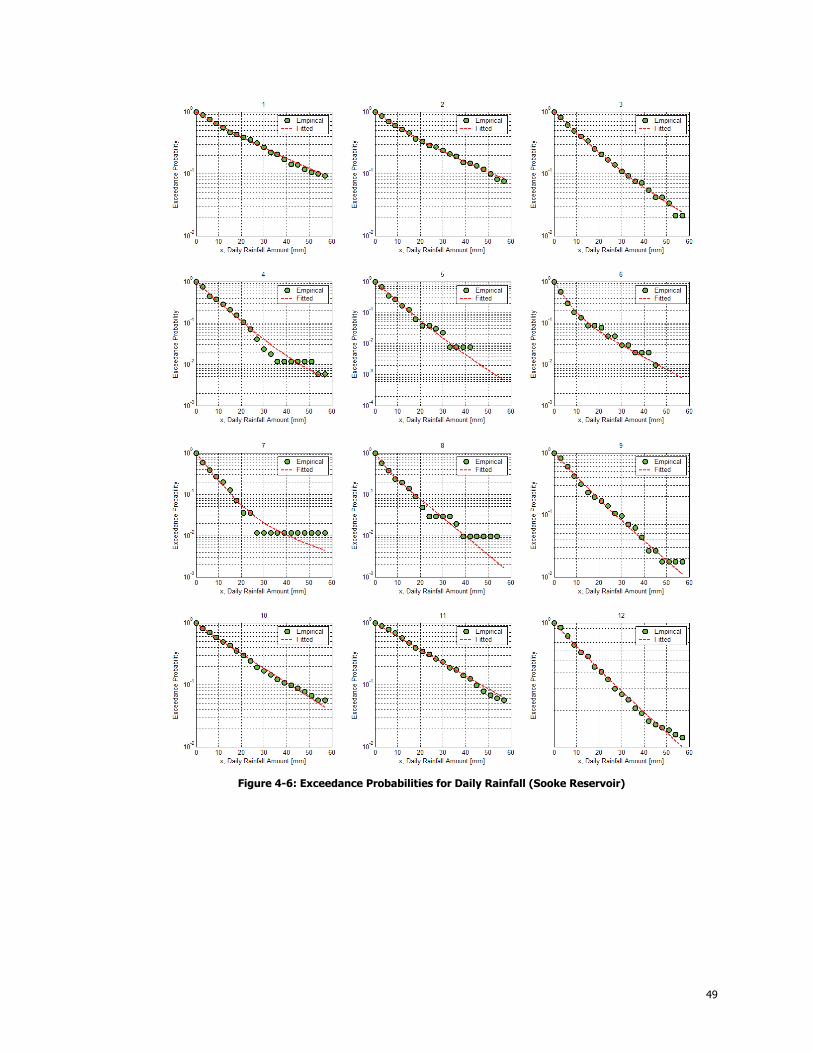
Figure 4-6: Exceedance Probabilities for Daily Rainfall (Sooke Reservoir)
49

Figure 4-7: Exceedance Probabilities for Daily Rainfall (Roxas City)
50

4.2.2 Fourier Series Fit to Parameter Sets
Two Markov Chain transitional probabilities (p00 and p10) and three mixed-exponential
parameters (p, µ1 and µ2) were generated for each month at each location. Thus, a total of
sixty parameters were needed to describe the rainfall process. Seasonal variability of each
parameter through the twelve months of the year was then represented by using maximum
likelihood estimates of the periodic parameters using five harmonics (Han, 2001). This
Fourier series fit is compared to the non-fitted transitional probabilities (Section 4.2.2.1) and
mixed-exponential parameters (Section 4.2.2.2).
As can be seen in Figures 4-8 to 4-10, the Fourier fits for all transitional probabilities are in
very close agreement. However, the parameter µ1 for Dorval (Figure 4-11), Sooke Dam
(Figure 4-12) and Roxas City (Figure 4-12) is not as well represented. Similarly, the Fourier
fit for p at Sooke Dam varies with the original estimate. This perhaps implies that lower
rainfall amounts may not be as well predicted.
An improvement of fit may be suggested by maximizing the variance explained using a
higher number of harmonics than the five used in this analysis for each parameter at each
location. This would however increase the total number of parameters needed to be
estimated (see Section 3.2.3). The use of five harmonics for all five parameters lowers the
total number of parameters needed in the model from sixty to fifty-five. According to Han
(2001), five harmonics were sufficient in explaining over 90% of the variance of monthly
parameters at Dorval.
The number of harmonics may of course be reduced and increased according to each
parameter set at each location to create a more parsimonious model but this was beyond the
scope of creating a general MCME model suited to various data from various locations. An
algorithm optimizing for the number of harmonics needed to explain maximum variance of
parameters from any location can always be incorporated in the model in future studies.
51

4.2.2.1 Transitional Probabilities
Figure 4-8: Monthly Transitional Probabilities and Fourier Series Fits (Dorval Airport)
Figure 4-9: Monthly Transitional Probabilities and Fourier Series Fits (Sooke Reservoir)
52

Figure 4-10: Monthly Transitional Probabilities and Fourier Series Fits (Roxas City)
53

4.2.2.2 Mixed-Exponential Parameters
Figure 4-11: Monthly Mixed-Exponential Parameters and Fourier Series Fits (Dorval Airport)
54

Figure 4-12: Monthly Mixed-Exponential Parameters and Fourier Series Fits (Sooke Reservoir)
55

Figure 4-13: Monthly Mixed-Exponential Parameters and Fourier Series Fits (Roxas City)
56

4.2.3 Simulation Verification
Following the calibration of rainfall amounts using Fourier fits of the mixed-exponential
Section 4.2.3.1 verifies the simulated daily rainfall amount. Sections 4.2.3.2 and 4.2.3.3 then
compares the simulated parameters from 100 simulations to the calibrated parameters
4.2.3.1 Generating Rainfall Amount from the CDF
Using the Fourier series parameters for the mixed-exponential cumulative density function
(CDF), for every wet day a random number between 0 to 1 was generated and the Newton-
Raphson algorithm was used to extract the rainfall amount.
To verify that this technique accurately derived the correct rainfall amount from the CDF,
the daily simulated amount (small trace dots) was plotted against the observed cumulative
probability (large dots) of rainfall (Figures 4-14 to 4-16). The simulated large dots were
expected to follow the empirical probability curve, which is indeed confirmed for all month
at all three locations.
For the months of January to March, November and December in Sooke Dam, it can be
seen that the simulated values are often higher than the empirical values. This is due to the
lack of observed rainfall amounts within the plotted rainfall range.
57

Figure 4-14: Simulated Rainfall and Observed Cumulative Distribution (Dorval Airport)
58

Figure 4-15: Simulated Rainfall and Observed Cumulative Distribution (Sooke Reservoir)
59

Figure 4-16: Simulated Rainfall and Observed Cumulative Distribution (Roxas City)
60

4.2.3.2 Simulated Transitional Probabilities
The boxplots in Figures 4-17 to 4-22 represent the spread of the transitional probabilities
computed from the 100 sets of monthly simulated data. Those are compared to the
empirical transition probabilities (represented by the dots connected by the dashed line).
It is apparent that the simulated transitional probabilities are well preserved and comparable
to the empirical values for all three locations. The median value of each boxplot is well
matched to the empirical value. The spread around the median in the boxplots represents
the variability that exists in 100 simulations over 20 years. The seasonal variability can also
be seen in general trend of the monthly boxplots for the whole year. Thus, it can be seen
that the simulation of daily rainfall occurrences is comparable to that of the observed
patterns.
A further investigation of the transitional probabilities at Dorval Airport shows that a day is
more likely to be dry if the previous day was dry in the months of April and October.
Similarly, there is a higher probability of rain on a given day in June, October and November
if the previous day was also rainy. There is also a clear periodic trend in these parameters.
At Sooke Dam, the likelihood of a dry day following another dry day increases from the
month of January till July, after which is declines to its lowest value in December. The
transitional probability of p10 also supports the fact that the winter months of November to
February contain the most rainy days in the year.
Figures 4-21 and 4-22 show the month of April as the driest month in Roxas City. This is
implied because the likelihood of a day being dry is the highest during this month, regardless
of the status of the previous day. The months of July to December seem to contain the
largest number of wet days due to their relatively low values of the transitional parameters.
Further analysis of the occurrence properties of simulated and observed data are provided in
Section 4.2.4.
61

Figure 4-17: Comparison between Simulated (Boxplots) and Empirical (o-- -o) p00 (Dorval Air.)
Figure 4-18: Comparison between Simulated and Empirical p10 (Dorval Air.)
62

Figure 4-19: Comparison between Simulated and Empirical p00 (Sooke Res.)
Figure 4-20: Comparison between Simulated and Empirical p10 (Sooke Res.)
63

Figure 4-21: Comparison between Simulated and Empirical p00 (Roxas City)
Figure 4-22: Comparison between Simulated and Empirical p10 (Roxas City)
64

4.2.3.3 Simulated Mixed-Exponential Parameters
When comparing simulated mixed-exponential parameters to the empirical (observed) values,
it can be seen that the simulated weighting parameters p for Dorval Airport (Figure 4-23), in
particular, varies greatly from the empirical values. In fact, for a majority of the months the
range of simulated values is very large, often spanning the entire feasible space (0 to 1) for
the parameter. For many cases (March, April, June, July, October and November) even the
middle 50% of simulated values in the boxplots do not match the empirical value. This is
also true for the simulation of the lower mean parameter µ1 (Figure 4-24) in the same
months. The simulated boxplots for the higher mean parameter µ2 (Figure 4-25), however
contain the empirical values and follows a similar trend.
In contrast, the median of the simulated boxplots and the empirical parameter values for
Sooke Reservoir and Roxas City show close agreement in value as well as the trend. There is
also a noticeable seasonal periodic variation in all parameters for these two locations. In
addition, there appears to be a higher distribution of rainfall with high means from the
months of June to November in Roxas City, while Sooke Reservoir the rainfall distribution
largely consists of a lower mean distribution.
The wide differences in simulated and empirical values for the mixed-exponential for Dorval
Airport and some months in Sooke Reservoir can be explained mainly due to the fact that
unlike the transitional probabilities which are estimated by the corresponding empirical
probabilities, the mixed-exponential parameters are estimated by the maximum likelihood
method. This procedure does not aim to preserve the specific observed mixed-exponential
parameters, but merely aims to find any parameter set that globally maximizes the likelihood
of matching the mixed-exponential function to the empirical distribution. Therefore, it is
expected that the generated rainfall series would provide a good match between the
simulated mixed-exponential function and the empirical distribution of rainfall amounts
rather than preserve the exact value of each mixed-exponential parameter independently.
65

Figure 4-23: Comparison between Simulated (Boxplots) and Empirical (o - - o) p (Dorval Airport)
Figure 4-24: Comparison between Simulated and Empirical µ1 (Dorval Airport)
66

Figure 4-25: Comparison between Simulated and Empirical µ2 (Dorval Airport)
Figure 4-26: Comparison between Simulated and Empirical p (Sooke Res.)
67

Figure 4-27: Comparison between Simulated and Empirical µ1 (Sooke Res.)
Figure 4-28: Comparison between Simulated and Empirical µ2 (Sooke Res.)
68

Figure 4-29: Comparison between Simulated and Empirical p (Roxas City)
Figure 4-30: Comparison between Simulated and Empirical µ1 (Roxas City)
69

Figure 4-31: Comparison between Simulated and Empirical µ2 (Roxas City)
4.2.4 Properties of Simulation and Observed Series
The statistical and physical properties of 100 simulations and the observed rainfall series
were compared, as described in the following:
4.2.4.1 Statistical Properties
Figures 4-32 to 4-37 show daily means and standard deviations of observed and simulated
rainfall series for each month at all three locations. The observed boxplot contains 20 values
for each year in the observed data period. Each monthly simulation boxplot contains 20
values for each year in the simulated period (twenty years) for every one of the 100
simulations, adding to a total of 2000 values in the boxplot.
A qualitative inspection of the boxplots shows that the medians of the means and standard
deviations of the simulations are comparable to the observed statistical characteristics. The
spread (middle 50%) of these characteristics are also very similar. Table 4-6 provides
quantitative percentage error difference between simulated and observed medians.
Although, it can be seen that most errors are less than 10% for all locations, the differences
in the months of January to April at Roxas City are very high (i.e. up to 400%). This is
mainly due to the observed data gaps during those months at that location.
70

Figure 4-32: Monthly Means of Daily Rainfalls (mm) for Dorval Airport
1 – Observed, 2 - Simulated
Figure 4-33: Monthly Std Deviations of Daily Rainfalls (mm) for Dorval Airport
1 – Observed, 2 - Simulated
71

Figure 4-34: Monthly Means of Daily Rainfalls (mm) for Sooke Reservoir
1 – Observed, 2 - Simulated
Figure 4-35: Monthly Std Deviations of Daily Rainfalls (mm) for Sooke Reservoir
1 – Observed, 2 - Simulated
72

Figure 4-36: Monthly Means of Daily Rainfalls (mm) for Roxas City
1 – Observed, 2 - Simulated
Figure 4-37: Monthly Std Deviations of Daily Rainfalls (mm) for Roxas City
1 – Observed, 2 - Simulated
73

74
Mean (mm) Standard Deviation (mm) Dorval obs sim 1 diff (%) obs sim 1 diff (%)
January 1.97 1.89 -3.91 3.63 3.96 9.01
February 1.58 1.76 11.59 3.92 3.87 -1.43
March 2.31 1.95 -15.68 5.69 4.50 -20.85
April 2.24 2.56 14.22 5.50 5.74 4.40
May 1.75 1.99 13.62 3.77 4.31 14.40
June 2.78 2.39 -14.04 5.68 5.27 -7.10
July 2.38 2.52 6.19 5.83 5.39 -7.54
August 2.91 3.06 5.16 6.84 6.62 -3.21
September 2.84 3.08 8.61 6.72 6.97 3.71
October 2.20 2.49 13.00 4.82 5.45 12.94
November 2.66 2.36 -11.28 5.20 4.61 -11.31
December 2.72 2.65 -2.50 4.82 5.12 6.12
MAE(%) 9.98 8.50
Mean (mm) Standard Deviation (mm) Sooke Reservoir obs sim 1 diff (%) obs sim 1 diff (%)
January 7.61 9.22 21.24 14.63 18.64 27.39
February 8.01 7.15 -10.71 14.88 14.68 -1.40
March 5.94 5.17 -12.98 9.97 10.68 7.20
April 2.52 2.73 8.31 5.34 6.29 17.62
May 1.31 1.11 -14.76 3.73 3.00 -19.58
June 1.09 1.00 -7.52 2.97 3.04 2.27
July 0.71 0.73 3.22 2.70 2.37 -12.20
August 0.74 1.03 38.39 2.97 3.28 10.57
September 2.17 1.88 -13.34 5.45 5.47 0.45
October 5.27 4.87 -7.61 11.88 11.29 -4.93
November 7.53 8.60 14.26 13.67 15.57 13.94
December 10.77 10.51 -2.49 18.18 18.84 3.68
MAE(%) 12.90 10.10
Mean (mm) Standard Deviation (mm) Roxas City obs sim 1 diff (%) obs sim 1 diff (%)
January 3.43 5.13 49.62 4.6139 10.18 120.64
February 1.26 3.15 151.02 3.6957 6.4549 74.66
March 0.97 3.34 244.50 2.2951 6.2897 174.05
April 0.54 2.96 442.92 2.1579 8.3857 288.60
May 3.48 5.51 58.11 7.8402 11.282 43.90
June 8.79 12.05 37.12 13.706 18.999 38.62
July 9.37 9.35 -0.18 11.732 13.2 12.51
August 7.60 9.28 22.09 12.49 15.022 20.27
September 8.74 8.59 -1.71 12.122 12.773 5.37
October 10.68 13.03 21.94 13.432 19.966 48.65
November 9.33 11.21 20.22 16.149 20.093 24.42
December 6.47 7.37 13.82 7.9988 11.38 42.27
MAE(%) 88.60 74.50 1 Simulated values correspond to mean of 100 simulations
Table 4-6: Numerical Comparison of Daily Median Statistical Properties

4.2.4.2 Physical Properties of Rainfall Series
Figures 4-38 to 4-49 show seasonal precipitation indices of the observed and simulated time
series at each location. In general, good agreements between observed and simulated
physical indices were found. Tables 4-7, 4-8 and 4-9 summarize the results in terms of the
percentage differences between median observed and simulated values (mean over the 100
simulated series).
Among the three locations, the seasonal properties from Dorval are best preserved with the
average percentage difference being less than 6% for any season. However, the differences
for the consecutive dry days during winter and spring are somewhat higher, 8.3% and 12.5%,
for these seasons, respectively. The errors for maximum 3-day rainfall total during summer
and autumn were 9.6% and 20.3%.
For Sooke Reservoir, the worst simulated property was the maximum 3-day rainfall total,
with differences exceeding 25% and 86% in winter and summer. All other seasonal indices
were well within 10% of the original median values.
Percentage of wet days for all four seasons during winter, spring, summer and autumn are
poorly simulated with median differences exceeding 52%, 110%, 39% and 42% respectively
for Roxas City. This could be largely due to the data missing for an entire year of the
calibrated observed series and some further data gaps within some months.
Overall, most simulated seasonal physical characteristic of rainfall are well preserved in the
MCME simulations. The best property simulated was the simple daily intensity index and
the 90th percentile of rainfall amounts at below 5% across the board.
75

Figure 4-38: Winter Indices (Dorval Airport): 1 – Observed, 2 - Simulated
Figure 4-39: Spring Indices (Dorval Airport): 1 - Observed, 2 - Simulated
76

Figure 4-40: Summer Indices (Dorval Airport): 1 – Observed, 2 - Simulated
Figure 4-41: Autumn Indices (Dorval Airport): 1 – Observed, 2 - Simulated
77

Figure 4-42: Winter Indices (Sooke Reservoir): 1 – Observed, 2 - Simulated
Figure 4-43: Spring Indices (Sooke Reservoir): 1 – Observed, 2 - Simulated
78

Figure 4-44: Summer Indices (Sooke Reservoir): 1 - Observed | 2 - Simulated
Figure 4-45: Autumn Indices (Sooke Reservoir): 1 – Observed, 2 - Simulated
79

Figure 4-46: Indices for December to February (Roxas City): 1 – Observed, 2 - Simulated
Figure 4-47: Indices for March to May (Roxas City): 1 – Observed, 2 - Simulated
80

Figure 4-48: Indices for June to August (Roxas City): 1 – Observed, 2 - Simulated
Figure 4-49: Indices for September to November (Roxas City): 1 – Observed, 2 - Simulated
81

Winter Spring Dorval obs sim 1 sim 1 diff (%) obs diff (%)
Prcp1 (%) 36.67 35.56 -3.03 28.80 30.43 5.66
SDII (mm) 6.03 6.15 2.02 7.62 7.43 -2.55
CDD (days) 8.00 9.00 12.50 12.00 11.00 -8.33
R3Days (mm) 29.50 27.82 -5.69 31.60 31.98 1.20
Prec90p (mm) 14.95 14.59 -2.41 17.84 17.41 -2.41
R90N (%) 9.09 10.00 10.00 10.00 9.76 -2.44
MAE (%) 5.94 3.77
Summer Autumn Dorval obs sim 1 sim 1 diff (%) obs diff (%)
Prcp1 (%) 32.07 31.52 -1.71 32.42 32.97 1.70
SDII (mm) 8.75 8.54 -2.34 7.95 8.29 4.34
CDD (days) 9.50 10.00 5.26 11.00 11.00 0.00
R3Days (mm) 37.85 34.21 -9.62 30.75 36.99 20.29
Prec90p (mm) 22.00 20.80 -5.45 18.48 19.32 4.55
R90N (%) 9.60 9.76 1.61 10.00 9.67 -3.33
MAE(%) 4.33 5.70 1 Simulated values correspond to mean of 100 simulations
Table 4-7: Numerical Comparison of Median Seasonal Indices (Dorval Airport)
Winter Spring Sooke Res. obs sim 1 sim 1 diff (%) obs diff (%)
Prcp1 (%) 41.11 40.00 -2.70 29.35 29.35 0.00
SDII (mm) 21.26 23.32 9.73 10.33 10.64 3.06
CDD (days) 11.00 10.00 -9.09 12.00 14.00 16.67
R3Days (mm) 106.70 134.13 25.71 51.35 58.54 13.99
Prec90p (mm) 52.24 55.68 6.58 22.35 25.46 13.88
R90N (%) 9.38 9.76 4.06 9.55 9.68 1.38
MAE (%) 9.65 8.16
Summer Autumn Sooke Res. obs sim 1 sim 1 diff (%) obs diff (%)
Prcp1 (%) 12.50 15.22 21.74 30.22 30.77 1.82
SDII (mm) 7.22 6.66 -7.63 18.12 16.98 -6.28
CDD (days) 27.00 22.00 -18.52 13.00 13.00 0.00
R3Days (mm) 11.10 20.68 86.31 97.40 93.18 -4.34
Prec90p (mm) 17.08 16.83 -1.44 39.39 41.44 5.19
R90N (%) 9.09 9.53 4.78 10.34 10.00 -3.26
MAE(%) 23.40 3.48 1 Simulated values correspond to mean of 100 simulations
Table 4-8: Numerical Comparison of Median Seasonal Indices (Sooke Reservoir)
82

December to February March to May Roxas City obs sim 1 sim 1 diff (%) obs diff (%)
Prcp1 (%) 44.44 67.78 52.50 21.20 44.57 110.25
SDII (mm) 7.62 8.06 5.79 8.92 9.36 4.93
CDD (days) 5.50 5.00 -9.09 11.00 10.00 -9.09
R3Days (mm) 63.70 84.82 33.16 34.90 74.47 113.38
Prec90p (mm) 18.32 19.82 8.24 28.74 26.53 -7.69
R90N (%) 10.20 10.00 -1.97 9.09 9.80 7.84
MAE (%) 18.46 42.20
June to August September to November Roxas City obs sim 1 sim 1 diff (%) obs diff (%)
Prcp1 (%) 53.80 75.00 39.39 53.85 76.92 42.86
SDII (mm) 13.08 13.84 5.83 14.65 14.68 0.21
CDD (days) 4.50 4.00 -11.11 4.00 3.00 -25.00
R3Days (mm) 93.40 126.42 35.35 122.95 145.73 18.53
Prec90p (mm) 37.31 37.61 0.81 37.62 39.12 3.99
R90N (%) 9.57 9.88 3.21 9.90 10.00 0.99
MAE(%) 15.95 15.26 1 Simulated values correspond to mean of 100 simulations
Table 4-9: Numerical Comparison of Median Seasonal Indices (Roxas City)
4.3 Performance of Hourly MCME Model
To assess the feasibility of the MCME model for hourly rainfall simulations, a modified
hourly MCME model was created and its performance assessed using hourly data from
Dorval Airport for the calibrated period from 1961-1980.
4.3.1 Fitting of Mixed-Exponential Distribution to Observed Data
Figure 4-50 shows the hourly distribution of rainfalls at increments of 0.6 mm from 0 to 5.1
mm. Although the fitted mixed-exponential curve fit most observed relative frequency
points well, the lowest interval from 0 to 0.3 mm is slightly underestimated.
The exceedance probability curves in Figure 4-51 provide evidence of multiple slopes,
especially in the months of January and May to November, further supporting the use of
mixed-exponentials in describing the distribution of hourly rainfall in the region.
83

Figure 4-50: Hourly Rainfall Distribution Fits using Monthly Parameters (x0.1 mm)
84

Figure 4-51: Exceedance Probability for Hourly Rainfall (x0.1 mm)
85

4.3.2 Fourier Series Fit to Parameter Sets
The Fourier fits (Figures 4-52 to 4-53) for the transitional probabilities and mixed-
exponential parameters are very close to originally derived parameters showing seasonal
variations as well. These hourly curve fits are in better agreement than that for the daily
parameters (especially, µ1 and µ2 parameters).
Figure 4-52: Monthly Transitional Probabilities and Fourier Series Fits for Hourly Rainfall
86

Figure 4-53: Monthly Mixed-Exponential Parameters and Fourier Series Fits for Hourly Rainfall
87

4.3.3 Simulation Verification
All computed parameters for the hourly MCME model fall within the simulated boxplots
and are in agreement to the median observed values. The probability of a dry hour following
dry hour is, as expected, very high (Figure 4-54). The highest chance for a wet hour
occurring following a dry hour, albeit very low still, is from May to October, whereas, a dry
hour following a wet hour is more likely in the months of June through to August. Similarly,
the probability of a dry hour following a wet hour is during the month of July (Figure 4-55).
These rainfall occurrence characteristics were well described by the MCME model.
As for the daily model, the simulated mixed-exponential parameters in the hourly model do
not always match the empirical values (Figures 4-56 to 4-58). The simulated middle 50% of
the boxplots for the weighted parameter p do not contain the calibrated value for February,
April and December, however, the other two mean parameters are well represented by the
simulations. There is also a clear seasonal periodic variation in the lower and higher means,
with the lower means staying hovering around 0.1 mm throughout the year.
Figure 4-54: Comparison between Simulated (Boxplots) and Empirical (o - - o) Hourly p00
88

Figure 4-55: Comparison between Simulated and Empirical Hourly p10
Figure 4-56: Comparison between Simulated and Empirical Hourly p
89

Figure 4-57: Comparison between Simulated and Empirical Hourly µ1
Figure 4-58: Comparison between Simulated and Empirical Hourly µ2
90

4.3.4 Properties of Simulated and Observed Rainfall Series
Figures 4-59 and 4-60 show the boxplots for the hourly means and standard deviations of
hourly rainfall for each month at Dorval Airport. Table 4-10 shows that percent difference
between all the simulated and observed medians are, on average, 18%. The differences
between simulated and observed means and standard deviations, however, are at their largest
between the months of May to July with differences exceeding 20%.
A further analysis was conducted to see whether the hourly rainfall data could be aggregated
or ‘lumped’ to form a daily rainfall equivalent. The simulated statistical and physical
properties of the daily rainfalls were then compared to the observed daily data from the same
period. Figures 4-61 and 4-62 show that the simulated lumped median values for the daily
mean and standard deviations are underestimated at an average of 32% and 38% difference,
respectively.
When comparing the physical properties of the hourly simulations (Figures 4-63 to 4-66), it
can be seen that the maximum number of consecutive dry hours (CDH) and maximum 8-
hour total rainfall (R8H) are underestimated at more than 25% for all four seasons. The
percentage of wet hours (Prcp1%) is the best simulated seasonal property, while the hourly
intensity index (equivalent to the daily SDII) shows less than 8% difference during spring,
summer and autumn (Table 4-11). In the comparison of lumped daily rainfall properties
(Figures 4-67 to 4-70), however, Prcp1% is worst captured by the lumped simulations when
compared to daily rainfall. Apart from the winter season, the median value of Prcp1% is
overestimated at a difference larger than 50% of the observed. The total 3-day total rainfall
(R3Days) is the only property that was simulated to less than 10% difference of the observed
value.
In summary, the MCME model could describe reasonably well the statistical and physical
properties of hourly rainfall series when its parameters were estimated using data at the same
hourly scale. However, this model was found not to be able to capture accurately the
properties of rainfall series for the daily scale from the ‘lumped’ hourly information. This
inconsistency should be investigated further using hourly rainfall data from other regions.
91

Figure 4-59: Monthly Means of Hourly Rainfalls (x 0.1 mm) 1 – Observed, 2 – Simulated
Figure 4-60: Monthly Standard Deviations of Hourly Rainfalls (x 0.1 mm)
1 – Observed, 2 – Simulated
92

Figure 4-61: Monthly Means of Lumped Daily Rainfalls (mm)
1 - Observed Daily, 2 – Lumped Daily
Figure 4-62: Monthly Std Deviations of Lumped Daily Rainfalls (mm)
1 - Observed Daily, 2 –Lumped Daily
93

Mean (0.1 x mm) Standard Dev (0.1 x mm) Hourly obs sim 1 sim 1 diff (%) obs diff (%)
January 0.19 0.29 49.64 1.60 2.83 76.60
February 0.19 0.16 -14.62 1.26 1.65 31.28
March 0.45 0.44 -3.00 3.07 3.05 -0.55
April 0.78 0.78 0.12 3.95 3.87 -2.11
May 0.68 0.86 25.15 3.67 4.38 19.45
June 1.16 0.90 -21.97 7.22 5.63 -22.07
July 1.01 1.21 19.93 7.15 8.63 20.66
August 1.28 1.17 -8.81 8.89 7.98 -10.21
September 1.09 1.38 27.16 7.27 8.57 17.83
October 1.02 0.89 -12.48 4.59 4.14 -9.68
November 0.80 0.90 12.34 4.16 4.38 5.05
December 0.39 0.32 -17.57 2.77 2.50 -9.75
MAE(%) 17.73 18.77
Mean (mm) Standard Deviation (mm) Lumped Daily obs sim 1 sim 1 diff (%) obs diff (%)
January 1.97 0.69 -64.80 3.63 2.10 -42.15
February 1.58 0.38 -75.75 3.92 1.18 -70.03
March 2.31 1.06 -54.14 5.69 2.37 -58.33
April 2.24 1.86 -16.74 5.50 3.01 -45.19
May 1.75 2.06 17.67 3.77 3.10 -17.75
June 2.78 2.16 -22.07 5.68 3.63 -35.98
July 2.38 2.91 22.46 5.83 5.26 -9.76
August 2.91 2.81 -3.25 6.84 4.86 -28.98
September 2.84 3.32 17.07 6.72 5.67 -15.69
October 2.20 2.14 -2.62 4.82 3.06 -36.66
November 2.66 2.17 -18.54 5.20 3.38 -34.95
December 2.72 0.78 -71.37 4.82 2.01 -58.28
MAE(%) 32.21 37.81 1 Simulated values correspond to mean of 100 simulations
Table 4-10: Numerical Comparison of Statistical Properties (Hourly and Lumped Daily)
94

Figure 4-63: Winter Indices (Hourly): 1 – Observed, 2 - Simulated
Figure 4-64: Spring Indices (Hourly): 1 – Observed, 2 – Simulated
95

Figure 4-65: Summer Indices (Hourly): 1 – Observed, 2 – Simulated
Figure 4-66: Autumn Indices (Hourly): 1 – Observed, 2 – Simulated
96

Figure 4-67: Winter Indices (Daily): 1 - Observed Daily, 2 – Lumped Daily
Figure 4-68: Spring Indices (Daily): 1 - Observed Daily, 2 – Lumped Daily
97
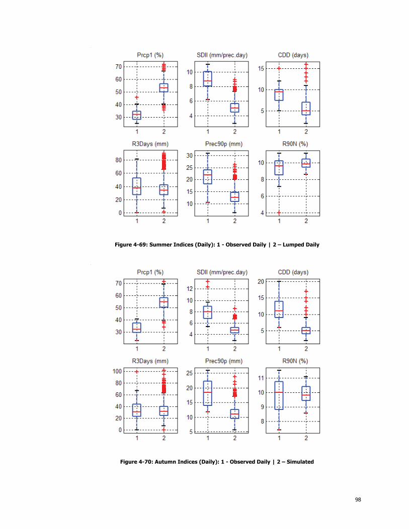
Figure 4-69: Summer Indices (Daily): 1 - Observed Daily | 2 – Lumped Daily
Figure 4-70: Autumn Indices (Daily): 1 - Observed Daily | 2 – Simulated
98

Winter Spring Hourly obs sim 1 sim 1 diff (%) obs diff (%)
Prcp (%) 2.45 2.43 -1.10 6.05 6.52 7.86
SDII (0.1xmm) 10.05 11.30 12.49 10.96 10.76 -1.87
CDH (hrs) 581.00 413.00 -28.92 325.00 211.50 -34.92
R8Hr (0.1xmm) 166.00 110.09 -33.68 186.00 118.66 -36.20
Prec90p (0.1xmm) 23.40 26.10 11.54 25.00 24.69 -1.24
R90N (%) 9.62 10.00 4.00 9.03 9.95 10.27
MAE (%) 15.29 15.40
Summer Autumn Hourly obs sim 1 sim 1 diff (%) obs diff (%)
Prcp% (%) 6.32 6.43 1.79 8.06 8.26 2.56
SDII (x0.1mm) 17.57 17.40 -1.00 11.96 12.86 7.52
CDH (hrs) 206.50 150.00 -27.36 257.50 148.00 -42.52
R8Hr (x0.1mm) 203.50 151.21 -25.70 205.50 143.12 -30.36
Pr90p (x0.1mm) 44.72 41.30 -7.66 24.78 28.42 14.70
R90N (%) 9.94 9.98 0.39 9.67 10.00 3.45
MAE(%) 10.65 16.85
Winter Spring Lumped Daily obs sim 1 sim 1 diff (%) obs diff (%)
Prcp (%) 36.67 18.64 -49.15 28.80 44.57 54.72
SDII (mm) 6.03 3.63 -39.72 7.62 3.81 -50.01
CDD (days) 8.00 16.00 100.00 12.00 8.00 -33.33
R3Days (mm) 29.50 11.98 -59.40 31.60 21.19 -32.96
Prec90p (mm) 14.95 8.64 -42.20 17.84 8.70 -51.20
R90N (%) 9.09 10.00 10.00 10.00 9.90 -0.98
MAE (%) 50.08 37.20
Summer Autumn Lumped Daily obs sim 1 sim 1 diff (%) obs diff (%)
Prcp% (%) 32.07 53.26 66.10 32.42 54.95 69.49
SDII (mm) 8.75 5.06 -42.13 7.95 4.70 -40.89
CDD (days) 9.50 5.00 -47.37 11.00 5.00 -54.55
R3Days (mm) 37.85 34.39 -9.15 30.75 31.23 1.54
Prec90p (mm) 22.00 12.70 -42.30 18.48 11.02 -40.37
R90N (%) 9.60 9.80 2.12 10.00 9.80 -1.96
MAE(%) 34.86 34.80 1 Simulated values correspond to mean of 100 simulations
Table 4-11: Numerical Comparison of Seasonal Indices (Hourly and Lumped Daily)
99

4.4 Annual Maximum Precipitation Analysis
The annual maximum precipitation (AMP) analysis was conducted on data from Dorval
Airport only since there were data gaps in the data from Roxas City. The methodology of
linking the MCME to the GCM-downscaled models outlined in Section 3.5 was applied to
data from Dorval Airport for the period of 1961-1980 for calibration and 1981-1990 for
validation.
4.4.1 Calibration of Combined Models
Figures 4-71 to 4-73 show the ranked AMP boxplots for the simulated outputs from the
MCME, downscaled-CGCM and downscaled-HadCM3. The dashed line plots the observed
AMP for the same period. MCME AMP boxplots clearly overestimate, while the
downscaled HadCM3 underestimate the observed values. Through graphical display, the
observed series falls best within the downscaled-CGCM AMP boxplots.
The weighted combination of the mean MCME and mean downscaled-HadCM3 provides
the closest agreement with the observed series, as shown in Figure 4-74. An optimal
weighting factor of 0.69 is applied to the mean MCME AMP series, while a factor of 0.31
was applied to the mean downscaled-HadCM3 series. Similarly, an optimal weighting factor
of 0.43 is applied to the mean MCME AMP series, while a factor of 0.57 was applied to the
mean downscaled-CGCM series (Figure 4-75). Table 4-12 shows the errors associated with
the AMP curves used in this calibration stage (as well as the validation period). The
combined mean MCME and mean downscaled-HadCM3 model provides the lowest MAE
and RMSE values of 2.83 mm and 3.40 mm.
Hence, the combination of the MCME-estimated AMPs and those given by the HadCM3
and CGCM could provide a good correction of bias in the estimation of AMPs at a local site.
Most importantly, this combination would provide a linkage between the MCME model with
a GCM model (downscaled values) for assessment of climate change impacts on AMPs at
local sites for future periods.
100

Figure 4-71: MCME - Ranked AMP Boxplots vs Observed Series (1961-1980)
Figure 4-72: CGCM - Ranked AMP Boxplots vs Observed Series (1961-1980)
Figure 4-73: HadCM3 - Ranked AMP Boxplots vs Observed Series (1961-1980)
101

Figure 4-74: Calibration of AMP Frequency Curves with HadCM3 (1961-1980)
Figure 4-75: Calibration of AMP Frequency Curves with CGCM (1961-1980)
102

4.4.2 Validation of Combined Models
Using the same weighting factors from the calibration stage, simulations from the MCME,
downscaled-CGCM and downscaled-HadCM3 models for the 1981-1990 period were used
to assess the feasibility of the proposed bias correction method in the estimation of AMPs at
Dorval Airport. Figures 4-76 to 4-78 show the comparison between the boxplots of
simulated AMPs and the observed AMPs for the validation period.
In general, it can be seen that the combined model (Figures 4-79 and 4-80) could provide a
better fit to the observed values, ie. the bias is reduced. More specifically, the downscaled-
HadCM3 boxplots (Figure 4-78) underestimate the observed series. The combined model of
the mean MCME and mean downscaled-HadCM3 (Figure 4-79) provides however a closer
fit to the observed as can be seen by the reduction of MAE and RMSE values in Table 4-12.
For the CGCM, the combined model of mean MCME and mean downscaled-CGCM
(Figure 4-80) did improve the bias of the MCME but did not significantly improve the bias
of the downscaled-CGCM. Nevertheless, the advantage of combining the GCM downscaled
values could provide a better tool in the study of the climate change impacts on extreme
precipitation characteristics at a local site as mentioned previously.
Calibration ('61-'80) Validation ('81-'90) Model 1
MAE RMSE MAE RMSE
MCME 3.00 3.77 4.35 4.08
HadCM3 3.52 4.94 5.66 4.69
MCME+HadCM3 2.83 3.40 4.23 3.56
Calibration ('61-'80) Validation ('81-'90) Model 2
MAE RMSE MAE RMSE
MCME 3.00 3.77 4.35 4.08
CGCM 3.16 3.71 3.72 3.01
MCME+CGCM 3.09 3.63 3.81 3.23
Table 4-12: Error Analysis of Simulated and Observed AMP Series
103

Figure 4-76: MCME - Ranked AMP Boxplots vs Observed Series (1981-1990)
Figure 4-77: CGCM - Ranked AMP Boxplots vs Observed Series (1981-1990)
Figure 4-78: HadCM3 - Ranked AMP Boxplots vs Observed Series (1981-1990)
104

Figure 4-79: Calibration of AMP Frequency Curves with HadCM3 (1981-1990)
Figure 4-80: Calibration of AMP Frequency Curves with CGCM (1981-1990)
105

5. Conclusions and Recommendations
. . . . . . . . . . . . . . . . . .
5.1 Conclusions
The main objective of the present study was to develop a stochastic model that could
accurately describe rainfall processes in different locations. The proposed model consists of
a combination of two components: the “rainfall occurrence” component, represented by the
first-order Markov Chain (MC), and the “rainfall amount” component, described by the
mixed-exponential (ME) distribution. The feasibility of the MCME model was tested using
daily rainfall data from different climatic conditions (Dorval Airport in Quebec and Sooke
Reservoir in British Columbia, Canada, and Roxas City in the Philippines) and hourly rainfall
data available at Dorval Airport for the 1961-1990 period. The main conclusions from the
present study are as follows:
1) The MCME model was found to be able to describe adequately the statistical and
physical properties of daily and hourly rainfall processes. More specifically, the
means and standard deviations and the precipitation indices of simulated series were
found to be in good to excellent agreement with the corresponding observed median
values (<10% difference in most cases). However, the number of consecutive dry
days and the maximum 3-day rainfall totals were not well preserved by the MCME
model, with larger than 20% difference for some seasons and locations.
2) The rainfall occurrence process can be well described by a Markov Chain for all
locations.
3) The rainfall amounts distributions can be well described by the mixed-exponential
distribution for all locations. In addition, the Shuffled Complex Evolution (SCE)
method was found to be the best method for estimating the mixed-exponential
parameters as compared to the Method of Moments, the local Direct Search
Complex optimization method, and the Multiple Guess Iterative optimization
method.
106

4) The Fourier series was found to be able to describe accurately the seasonality of the
MCME model parameters, especially the transitional probabilities.
5) In comparison to the daily model, the hourly MCME model for Dorval Airport,
produced larger errors between observed and simulated data series, even though the
hourly data showed a better fit to the mix-exponential function. The number of
maximum consecutive dry hours and maximum 8-hour rainfall amount were not well
simulated by the model for some seasons. In addition, inconsistency was found
regarding the description of daily rainfall characteristics using the hourly-calibrated
MCME model.
6) A combined weighted model of the annual maximum precipitation (AMP) series of
the MCME model and downscaled-GCM models (using a regression based method)
provided an efficient and practical method for correcting the bias of calibrated data
simulations in order to achieve a good agreement between downscaled-GCM AMPs
and the observed AMPs at a local site. Furthermore, this combination could provide
a necessary linkage between the MCME model and the downscaled-GCM outputs
for climate change impact assessment studies.
In summary, given sufficient rainfall time series data for any location, the daily MCME model
is capable of calibrating to that observed series and simulating any number of synthetic series
of any length of time. The calibrated model could preserve adequately the observed
statistical and physical characteristics of the underlying rainfall process, over at least the
temperate and tropical areas analyzed in this study.
5.2 Recommendations for Future Work
Several recommendations may be suggested for improving the modeling and programming
structure of the MCME model in this study.
107

Reducing Parameters
As mentioned earlier, the current model allows the use of a fixed number of harmonics (five)
to describe the Fourier series fit to the estimated parameters. However, the model may be
made more parsimonious by determining the number of significant harmonics, based on
cumulative periodograms (Salas et al., 1980) and reducing the number of parameters required
for all twelve months and all locations. This involves considerable programming complexity
where the generalized model will need to find the optimal number of harmonics and
calibrate given any set of data.
Temporal Downscaling
To produce synthetic rainfall data from the 24 hour scale to the 5 minute scale, the hourly
MCME model was examined. However, at lower time scales, the first order Markov chain
dependency for the transitional probabilities may not be sufficient to represent the strong
persistence of rainfall occurrence. Therefore, higher order Markov Chains should be
investigated when modeling the MCME for shorter time scales. Although mixed exponential
works well for the hourly scale, other distributions should also be studied at shorter time
scales to see what could provide the most acceptable fit with observed amounts.
MCME models may also be developed at each time scale to see whether scaling relationships
exist for different parameters from the daily time step to the 5 minute step. This would
allow researchers and engineers the ability to simulate rainfall through temporal downscaling,
at time scales where the observed data are not available or insufficient. There is, however
more computational difficulties associated with smaller time steps creating larger data
processing problems.
108

Effect of Climate Change
The effect of climate change on rainfall patterns may be incorporated into the MCME model
by adjusting the five MCME parameters directly. Regression downscaling techniques linking
climate variables outputted from GCMs to local mixed-exponential parameters and
transitional probabilities could provide one such method. Another method may involve the
calibration of parameters using consecutive 5 to 10-year periods and noting the trend in
changing parameters. This trend may then be used to extrapolate the parameters to a future
time and applied by ‘brute force’ to the model. However, more research is required to know
whether climate change affects rainfall occurrence or amounts or both at the local scale. The
question of how site specific the effect of climate change is when affecting the rainfall
process must also be answered.
The MCME model must be further developed to incorporate change in climate variability,
over various areas, in the mixed-exponential part of the model. The effect of large scale
variability (Wilby et al., 2002b), i.e., NAO, ENSO, etc. should be considered.
Predicting the Annual Maximum Precipitation Series
It must be noted that the combined weighted AMP series presented in this study was
calibrated to only one sample of observed data and must be tested in other areas. Therefore,
the combined model cannot provide any measure of uncertainty when predicting AMPs. A
bootstrapping technique may be used in future studies to provide a confidence interval for
the observed series and then used in the calibration of any MCME and downscaled GCM
AMP series. Data from longer periods should also be used to eliminate discontinuities in the
observed series for better calibration.
. . . . . . . . . . . . . . . . . .
109

6. References
. . . . . . . . . . . . . . . . . .
Buishand, T.A. 1977. Stochastic Modeling of Daily Rainfall Sequences. Medidlingen
Landbouwhogeschool Wageningen 77-3.
Campbell, G.S. 1990. CLIMGEN, A program that Generates Weather Data (Precipitation,
Maximum and Minimum Temperature). Unpublished.
Cox, D.R., and V. Isham. 1988. A Simple Spatial Model of Rainfall. Proceedings of the Royal
Society London A415: 317-328.
Chin, E.H. 1977. Modeling Daily Precipitation Occurrence Process with Markov Chain. Water
Resources Research 13(6): 949-956.
Cooke, D.S. 1953. The Duration of Wet and Dry Spells at Moncton, New Brunswick. Quarterly
Journal of the Royal Meteorological Society 79(342): 536-538.
Cowpertwait, P.S.P. 1995. A Generalized Spatial-Temporal Model of Rainfall Based on a Clustered
Point Process. Proceedings: Mathematical and Physical Sciences 450(1938): 163-175.
Cunnane, C. 1978. Unbiased Plotting Positions - A Review. Journal of Hydrology 37(3/4).
Danuso, F. 2002. Climak: A Stochastic Model for Weather Data Generation. Ital. J. Agron 6:57-71.
Delleur, J.W., and M.L. Kavvas. 1978. Stochastic Models for Monthly Rainfall Forecasting and
Synthetic Generation. Journal of Applied Meteorology 17(10): 1528-1536.
Duan, Q., S. Sorooshian, and V.K. Gupta. 1992. Effective and Efficient Global Optimization for
Conceptual Rainfall-Runoff Models. Water Resources Research. 28(4): 1015-1031.
110

Duan, Q., S. Sorooshian, and V.K. Gupta. 1994. Optimal Use of the SCE-UA Global
Optimization Method for Calibrating Watershed Models. Journal of Hydrology. 158: 265-284.
Dubrovsky, M. 1997. Creating Daily Weather Series with the Use of the Weather Generator.
Environmetrics. 8: 409-424.
Dumont, A.G., and D.S. Boyce. 1974. The probabilistic simulation of weather variables. Journal of
Agricultural Engineering Research 19:131-145.
Elsner, J.B., and A.A. Tsonis. 1993. Complexity and predictability of hourly precipitation. Journal of
the Atmospheric Sciences 50(3).
Entekhabi,D., and P.S. Eagleson. 1989. Land Surface Hydrology Parameterization for Atmospheric
General Circulation Models Including Subgrid Scale Spatial Variability. Journal of Climate JLCLEL
2(8).
Everitt, B.S., and D.J. Hand. 1981. Finite Mixture Distributions. Monographs on Applied
Probability and Statistics, London: Chapman and Hall.
Feyerherm, A.M., and L.D. Bark. 1967. Goodness of Fit of a Markov Chain Model for Sequences of
Wet and Dry Days. Journal of Applied Meteorology 6(5): 770-773.
Fitzpatrick, E.A., and A. Krishnan. 1967. A First-order Markov model for Assessing Rainfall
Discontinuity in Central Australia. Theoretical and Applied Climatology 15(3): 242-259.
Foufoula-Georgiou, E., and P. Guttorp. 1987. Assessment of a class of Neyman-Scott models for
temporal rainfall. Journal of Geophysical Research 92(D8): 9679-9682.
Gabriel, K. R., and J. Neumann. 1961. A Markov Chain Model for Daily Rainfall Occurence at Tel
Aviv. Quarterly Journal of Royal Meteorology Society 88: 90-95.
111

Gachon, P., A. St-Hilaire, T. Ouarda, V.T.V Nguyen, C. Lin, and J. Milton. 2005. A first
evaluation of the strength and weaknesses of statistical downscaling methods for simulating extremes over
various regions of eastern Canada. Subcomponent, Climate Change Action Fund (CCAF),
Environment Canada, Final report, Montréal, QC 209.
Gates, P., and H. Tong. 1976. On Markov Chain Modeling to Some Weather Data. Journal of
Applied Meteorology 15: 1145-51.
Geng, S. 1988. A Program to Simulate Meteorological Variables: Documentation for SIMMETEO.
University of California, Agricultural Experiment Station.
Geng, S., and P. de Vries. 1986. Simple Method for Generating Daily Rainfall Data. Agricultural
and Forest Meteorology 36(4).
Giorgi, F., and L.O. Mearns. 1999. Introduction to special section: Regional climate modeling revisited.
Journal of Geophysical Research 104(D6): 6335-6352.
Greenwood, J.A., and D. Durand. 1960. Aids for Fitting the Gamma Distribution by Maximum
Likelihood. Technometrics 2(1): 55-65.
Gregory, J.M., T.M. Wigley, and P.D. Jones. 1993. Application of Markov Models to Area-Average
Daily Precipitation Series and Interannual Variability in Seasonal Totals. Climate Dynamics 8: 299-
310.
Gyasi-Agyei, Y., and G.R. Willgoose. 1997. A Hybrid Model for Point Rainfall Modeling. Water
Resources Research 33(7): 1699-1706.
Haan, C.T., D.M. Allen, and J.O. Street. 1976. A Markov Chain Model of Daily Rainfall. Water
Resources Research 12: 443-449.
Han, S-Y. 2001. Stochastic Modeling of Rainfall Processes: A Comparative Study Using Data from
Different Climatic Conditions. Masters Thesis, McGill University, QC.
112

Hanson, C.L., K.A. Cumming, D.A. Woolhiser, and C.W. Richardson. 1994. Microcomputer
Program for Daily Weather Simulation in the Contiguous United States. Agricultural Research Service
114.
Haylock, M.R., and C.M. Goodess. 2004. Interannual Variability of Extreme European Winter
Rainfall and Links with Mean Large-Scale Circulation. International Journal of Climatology
24:759-776.
Hershfield, D.M. 1970. The Frequency and Intensity Of Wet And Dry Seasons And Their
Interrelationships. Water Resources Bulletin.
Hutchinson, M.F. 1995. Interpolating Mean Rainfall Using Thin Plate Smoothing Splines.
International Journal of Geographical Information Science 9(4): 385-403.
Ison, N.T., A.M. Feyerherm, and L.D. Bark. 1971. Wet Period Precipitation and the Gamma
Distribution. Journal of Applied Meteorology 10(4): 658-665.
Johnson, G.L., C. Daly, G.H.Taylor, and C.L. Hanson. 2000. Spatial variability and interpolation
of stochastic weather simulation model parameters. Journal of Applied Meteorology 39(6): 778-796.
Jones, P.G., and P.K. Thornton. 1997. Spatial and Temporal Variability of Rainfall Related to a
Third-Order Markov Model. Agricultural and Forest Meteorology 86: 127-138
Katz, R.W. 1977. Precipitation as a Chain-Dependent Process. Journal of Applied Meteorology 16:
671-76.
Kavvas, M.L., and J.W. Delleur. 1981. A Stochastic Cluster Model of Daily Rainfall Sequences.
Water Resources Research 17(4): 1151-1160.
Khaliq, M.N., and C. Cunnane. 1996. Modelling point rainfall occurrences with the modified Bartlett-
Lewis rectangular pulses model. Journal of Hydrology 180(1-4): 109-138.
113

Kilsby, C.G., C.S. Fallows, and P.E. O'Connell. 1998. Generating rainfall scenarios for hydrological
impact modelling. Hydrology in a Changing Environment 1:33-42.
Kotz, S., and J. Neumann. 1963. On the Distribution of Precipitation Amounts for Periods of
Increasing Length. Journal of Geophysical Research 68:3635.
Lall, U., B. Rajagopalan, and D.G. Tarboton. 1996. A nonparametric wet/dry spell model for
resampling daily precipitation. Water Resources Research 32(9): 2803-2823.
Le Cam, L. 1961. A Stochastic Description of Precipitation. Proceedings of the 4th Berkeley
Symposium on Mathematical Statistics and Probability. University of California, Berkley.
Mearns, L. O., R.W. Katz, and S.H. Schneider. 1984. Changes in the probabilities of extreme high
temperature events with changes in global mean temperature. Journal of Climate and Applied
Meteorology 23:1601-1613.
Mielke, P.W. 1973. Another family of distributions for describing and analyzing precipitation data
(Asymmetric positively skewed distributions family for precipitation data analysis, using two-sample
nonparametric test). Journal of Applied Meteorology 12:275-280.
Nelder, J.A., and R. Mead. 1965. A simplex method for function minimization. Computer Journal
7(4): 308-313.
Nguyen, V.T.V., and A. Mayabi. 1990. Probabilistic Analysis of Summer Daily Rainfall for the
Montreal Region. Canadian Water Resources Journal 15(3).
Nguyen, V.T.V., and J. Rousselle. 1982. Probabilistic Characterization of Point and Mean Areal
Rainfalls. Time Series Methods in Hydrosciences. Proceedings of an International Conference held
at Canada Centre for Inland Waters October 6-8, 1981, Burlington, Ontario. Developments
in Water Science 17.
114

Nguyen, V.T.V., T.D. Nguyen, and P. Gachon. 2005. An evaluation of statistical downscaling
methods for simulating daily precipitation and extreme temperature series at a local site. Environmental
Hydraulics and Sustainable Water Management 1:1911-1916.
Nicks, A.D., and G.A. Gander. 1994. CLIGEN: A weather generator for climate inputs to water
resource and other models. Proceedings of the 5th International Conference on Computers in
Agriculture 3-94.
Pavlopoulos, H., and B. Kedem. 1992. Stochastic modeling of rain rate processes: a diffusion model.
Communications in Statistics. Stochastic Models 8(3): 397-420.
Peyron, N., and V.T.V. Nguyen. 2004. A Systematic Assessment of Global Optimization Methods for
Conceptual Hydrologic Models Calibration. American Geophysical Union, Spring Meeting H52A-
02.
Rajagopalan, B., U. Lall, D.G. Tarboton, and D.S. Bowles. 1997. Multivariate nonparametric
resampling scheme for generation of daily weather variables. Stochastic Environmental Research and
Risk Assessment 11(1): 65-93.
Rascko, P., L. Szeidl, and M. Semenov. 1991. A Serial Approach to Local Stochastic Weather
Models. Ecological Modelling 57: 27-41.
Richardson, C.W. 1981. Stochastic Simulation of Daily Precipitation, Temperature, and Solar
Radiation. Water Resources Research 17(1): 182-190.
Richardson, C.W., and D.A. Wright. 1984. WGEN: A Model for Generating Daily Weather
Variables. Agriculture Research Service 8.
Rider, P.R. 1961. The Method of Moments Applied to a Mixture of Two Exponential Distributions.
The Annals of Mathematical Statistics 32(1): 143-147.
115

Rodríguez-Iturbe, I., B.F. De Power, and J.B. Valdés. 1987. Rectangular pulses point process models
for rainfall: Analysis of empirical data. Journal of Geophysical Research 2(D8): 9645-9656.
Roldan, J., and D. Woolhiser. 1982. Stochastic Daily Precipitation Models. I. A Comparison of
Occurrence Processes. Water Resources Research 18(5): 1451-1459.
51-1459.
Salas, J.D., J.W. Delleur, V. Yevjevich, and W.L. Lane. 1980. Applied Modeling of Hydrological
Time Series. Water Reources Publications, Littleton, Colorado.
Semenov, M.A., R.J. Brooks, E.M. Barrow, and C.W. Richardson. 1998. Comparison of the
WGEN and LARS-WG stochastic weather generators for diverse climates. Climate Research 10(1):
95-107.
Semenov, M.A., and E.M. Barrow. 1997. Use of a Stochastic Weather Generator in the Development
of Climate Change Scenarios. Climatic Change 35(4): 397-414.
Semenov, M.A., and J.R. Porter. 1995. Climatic Variability and the Modelling of Crop Yields.
Agricultural and Forest Meteorology 73: 765-783
Soltani, A., and G. Hoogenboom. 2003. A statistical comparison of the stochastic weather generators
WGEN and SIMMETEO. Climate Research 24: 215-230.
Srikanthan, R., and T.A. McMahon. 1982. Stochastic Generation of Monthly Streamflows. Journal of
the Hydraulics Division 108(3): 419-441.
Stern, R.D., and R. Coe. 1984. A Model Fitting Analysis of Daily Rainfall Data. Journal of the
Royal Statistical Society Series 147(A): 1-34.
Todorovic, P., and D.A. Woolhiser. 1975. A Stochastic Model of n-day Precipitation. Journal of
Applied Meteorology 14: 17-24.
116

Waymire, E.D., and V.K. Gupta. 1981. The Mathematical Structure of Rainfall Representations 1. A
Review of the Stochastic Rainfall Models. Water Resources Research 17(5): 1261-1272.
Waymire, E., V.K. Gupta, and I. Rodriguez-Iturbe. 1984. Spectral Theory of Rainfall Intensity at
the Meso-beta Scale. Water Resources Research 20(10).
Wilby, R.L., and T. M.L. Wigley. 1997. Downscaling general circulation model output: a review of
methods and limitations. Progress in Physical Geography 21(4): 530.
Wilby, R.L., C.W. Dawson, and E.M. Barrow. 2002a. SDSM - A Decision Support Tool for the
Assessment of Regional Climate Change Impacts. Environmental Modelling and Software 17(2):
145-157.
Wilby, R.L., D. Conway, and P.D. Jones. 2002b. Prospects for downscaling seasonal precipitation
variability using conditioned weather generator parameters. Hydrological Processes 16(6): 1215-1234.
Wilks, D.S. 1999. Interannual variability and extreme-value characteristics of several stochastic daily
precipitation models. Agricultural and Forest Meteorology 93(3): 153-169.
Wilks, D.S. 1992. Adapting Sochastic Weather Generation Algorithms for Climate Change Studies.
Climate Change 22: 67-84.
Wilks, D.S., and R.L. Wilby. 1999. The Weather Generation Game: A Review of Stochastic Weather
Models. Progress in Physical Geography 23(3): 329-357.
Woolhiser, D.A., and G.G.S. Pegram. 1978. Maximum Likelihood Estimation of Fourier Coefficient
to Describe Seasonal Variations of Parameters in Stochastic Daily Precipitation Models. Journal of
Applied Meteorology 18: 34-42.
Young, K.C. 1994. A multivariate chain model for simulating climatic parameters from daily data.
Journal of Applied Meteorology 33(6).
117

118
Zhang, Q., B. Singh, S. Gagnon, J. Rousselle, N. Evora, S. Weyman. 2004. The Application of
WGEN to Simulate Daily Climatic Data for Several Canadian Stations. Canadian Water Resources
Journal 29(1): 59-72.
. . . . . . . . . . . . . . . . . .