quantitative data analysis - open university of hong kong on quantitative data analysis.pdf ·...
TRANSCRIPT

Seminar on
Quantitative Data Analysis:Quantitative Data Analysis:SPSS and AMOS
Miss Brenda Lee2:00p.m. – 6:00p.m.
24th July, 2015The Open University of Hong Kong
SBAS (Hong Kong) Ltd. ‐ All Rights Reserved. 1
AgendaAgenda
• MANOVA, Repeated Measures ANOVA, Linear Mixed Models
– Demo and Q&A
• EFA
– Demo and Q&ADemo and Q&A
• CFA and SEM
– Demo and Q&A
SBAS (Hong Kong) Ltd. ‐ All Rights Reserved. 2
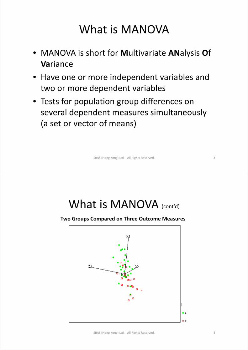
What is MANOVAWhat is MANOVA
• MANOVA is short for Multivariate ANalysis Of Variance
• Have one or more independent variables and two or more dependent variablestwo or more dependent variables
• Tests for population group differences on several dependent measures simultaneously(a set or vector of means)(a set or vector of means)
SBAS (Hong Kong) Ltd. ‐ All Rights Reserved. 3
What is MANOVAWhat is MANOVA (cont’d)Two Groups Compared on Three Outcome Measures
SBAS (Hong Kong) Ltd. ‐ All Rights Reserved. 4
MANOVA AssumptionsMANOVA Assumptions
• Large samples or multivariate normality
• Homogeneity of the within group variance ‐Homogeneity of the within group variance covariance matrices (Box’s M test)
R id l ( ) f ll l i i l• Residuals (errors) follow a multivariate normal distribution in the population
• Linear model (additivity, independence between the error and model effectbetween the error and model effect, independence of the errors)
SBAS (Hong Kong) Ltd. ‐ All Rights Reserved. 5
What to Look for in MANOVAWhat to Look for in MANOVA
• Multivariate statistical tests
• Post hoc test on marginal means (univariatePost hoc test on marginal means (univariateonly)
T 1 h h T 4 f• Type 1 through Type 4 sums of squares
• Specify Multiple Random Effect models, if p y p ,necessary
R id l di t d l d i fl• Residuals, predicted values and influence measures
SBAS (Hong Kong) Ltd. ‐ All Rights Reserved. 6
General Linear Model in SPSSGeneral Linear Model in SPSS
G l Li M d l• General Linear Model– Factors and covariates are assumed to have linear relationships to the dependent variable(s)relationships to the dependent variable(s)
• GLM Multivariate procedure– Model the values of multiple dependent scaleModel the values of multiple dependent scale variables, based on their relationships to categorical and scale predictors
• GLM Repeated Measures procedure– Model the values of multiple dependent scale
i bl d t lti l ti i d b dvariables measured at multiple time periods, based on their relationships to categorical and scale predictors and the time periods at which they were measured.
SBAS (Hong Kong) Ltd. ‐ All Rights Reserved. 7
MANOVA ResultsMANOVA Results
• Multivariate Tests
– Pillai's trace is a positive‐valued statistic. pIncreasing values of the statistic indicate effects that contribute more to the model.
– Wilks' Lambda is a positive‐valued statistic that ranges from 0 to 1 Decreasing values of theranges from 0 to 1. Decreasing values of the statistic indicate effects that contribute more to the modelthe model.
SBAS (Hong Kong) Ltd. ‐ All Rights Reserved. 8
MANOVA ResultsMANOVA Results (cont’d)
H lli ' i h f h i l f– Hotelling's trace is the sum of the eigenvalues of the test matrix. It is a positive‐valued statistic for which increasing values indicate effects thatwhich increasing values indicate effects that contribute more to the model.
Roy's largest root is the largest eigenvalue of the– Roy s largest root is the largest eigenvalue of the test matrix. Thus, it is a positive‐valued statistic for which increasing values indicate effects thatwhich increasing values indicate effects that contribute more to the model.
There is evidence that Pillai's trace is more robustThere is evidence that Pillai s trace is more robust than the other statistics to violations of model assumptionsp
SBAS (Hong Kong) Ltd. ‐ All Rights Reserved. 9
Post Hoc TestsPost Hoc Tests• LSD
The LSD or least significant difference method simply applies standard t tests to allThe LSD or least significant difference method simply applies standard t tests to all possible pairs of group means. No adjustment is made based on the number of tests performed. The argument is that since an overall difference in group means has already been established at the selected criterion level (say 05) no additional control isbeen established at the selected criterion level (say .05), no additional control is necessary. This is the most liberal of the post hoc tests.
• SNK, REGWF, REGWQ & Duncan
The SNK (Student‐Newman‐Keuls), REGWF (Ryan‐Einot‐Gabriel‐Welsh F), REGWQ (Ryan‐Einot‐Gabriel‐Welsh Q, based on the studentized range statistic) and Duncan methods involve sequential testing. After ordering the group means from lowest to highest, the q g g g p g ,two most extreme means are tested for a significant difference using a critical value adjusted for the fact that these are the extremes from a larger set of means. If these means are found not to be significantly different, the testing stops; if they are different then the testing continues with the next most extreme set, and so on. All are more conservative than the LSD. REGWF and REGWQ improve on the traditionally used SNK in that they adjust for the slightly elevated false‐positive rate (Type I error) that SNK has when the set of means tested is much smaller than the full set.
SBAS (Hong Kong) Ltd. ‐ All Rights Reserved. 10

Post Hoc TestsPost Hoc Tests (cont’d)
f i & Sid k• Bonferroni & Sidak
The Bonferroni (also called the Dunn procedure) and Sidak (also called Dunn‐Sidak) perform each test at a stringent significance level to insure that the family‐wise (applying to the set of tests) false‐positive rate does not exceed the specified value. They are based on inequalities relating the probability of a false‐positive result on each individual test to the probability of one or more false positives for a set of i d d t t t F l th B f i i b d dditi i litindependent tests. For example, the Bonferroni is based on an additive inequality, so the criterion level for each pairwise test is obtained by dividing the original criterion level (say .05) by the number of pairwise comparisons made. Thus with five means and therefore ten pairwise comparisons each Bonferroni test will befive means, and therefore ten pairwise comparisons, each Bonferroni test will be performed at the .05/10 or .005 level.
• Tukey (b)
The Tukey (b) test is a compromise test, combining the Tukey (see next test) and the SNK criterion producing a test result that falls between the two.
SBAS (Hong Kong) Ltd. ‐ All Rights Reserved. 11
Post Hoc TestsPost Hoc Tests (cont’d)
k• Tukey
Tukey’s HSD (Honestly Significant Difference; also called Tukey HSD, WSD, or Tukey(a) test) controls the false‐positive rate family‐wise. This means if you are testing at the .05 level, that when performing all pairwise comparisons, the probability of obtaining one or more false positives is .05. It is more conservative than the Duncan and SNK. If all pairwise comparisons are of interest, which is
ll th T k ’ t t i f l th th B f i d Sid kusually the case, Tukey’s test is more powerful than the Bonferroni and Sidak.
• Scheffe
Scheffe’s method also controls the family‐wise error rate. It adjusts not only for the pairwise comparisons, but also for any possible comparison the researcher might ask. As such it is the most conservative of the available methods (false‐positive rate is least), but has less statistical power.
SBAS (Hong Kong) Ltd. ‐ All Rights Reserved. 12
Specialized Post Hoc TestsSpecialized Post Hoc Tests
hb ’ G 2 & G b i l l• Hochberg’s GT2 & Gabriel: Unequal Ns
Most post hoc procedures mentioned above (excepting LSD, Bonferroni & Sidak) were derived assuming equal group sample sizes in addition to homogeneity of variance and normality of error. When the subgroup sizes are unequal, SPSS substitutes a single value (the harmonic mean) for the sample size. Hochberg’s GT2 and Gabriel’s post hoc test explicitly allow for unequal sample sizes.
• Waller‐Duncan
The Waller‐Duncan takes an approach (Bayesian) that adjusts the criterion value pp ( y ) jbased on the size of the overall F statistic in order to be sensitive to the types of group differences associated with the F (for example, large or small). Also, you can specify the ratio of Type I (false positive) to Type II (false negative) error in the test. This feature allows for adjustments if there are differential costs to the two types of errors.
SBAS (Hong Kong) Ltd. ‐ All Rights Reserved. 13
Unequal Variances and Unequal Ns and Selection of Post Hoc Tests
• Tamhane T2, Dunnett’s T3, Games‐Howell, Dunnett’s C
Each of these post hoc tests adjust for unequal variances and sample sizes in the groups. Simulation studies (summarized in Toothaker, 1991) suggest that although G H ll b t lib l h th i l d lGames‐Howell can be too liberal when the group variances are equal and sample sizes are unequal, it is more powerful than the others.
An approach some analysts take is to run both a liberal (say LSD) and a conservative (Scheffe or TukeyHSD) post hoc test. Group differences that show up under both criteria are considered solid findings, hil h f d diff l d h lib lwhile those found different only under the liberal
criterion are viewed as tentative results.
SBAS (Hong Kong) Ltd. ‐ All Rights Reserved. 14
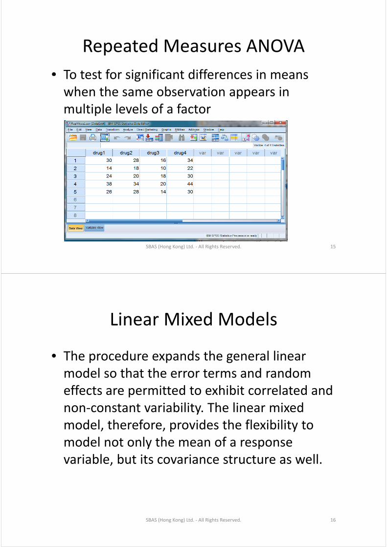
Repeated Measures ANOVARepeated Measures ANOVA
• To test for significant differences in meansTo test for significant differences in means when the same observation appears in
lti l l l f f tmultiple levels of a factor
SBAS (Hong Kong) Ltd. ‐ All Rights Reserved. 15
Linear Mixed ModelsLinear Mixed Models
• The procedure expands the general linear model so that the error terms and random effects are permitted to exhibit correlated and non‐constant variability The linear mixednon constant variability. The linear mixed model, therefore, provides the flexibility to model not only the mean of a responsemodel not only the mean of a response variable, but its covariance structure as well.
SBAS (Hong Kong) Ltd. ‐ All Rights Reserved. 16
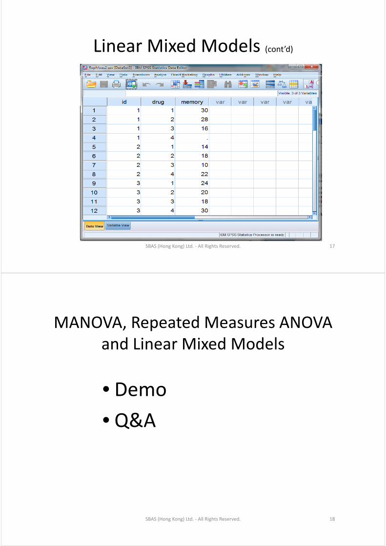
Linear Mixed ModelsLinear Mixed Models (cont’d)
SBAS (Hong Kong) Ltd. ‐ All Rights Reserved. 17
MANOVA R t d M ANOVAMANOVA, Repeated Measures ANOVA and Linear Mixed Modelsand Linear Mixed Models
• Demo
• Q&A
SBAS (Hong Kong) Ltd. ‐ All Rights Reserved. 18
Exploratory Factor AnalysisExploratory Factor Analysis
• The purpose of data reduction is to remove redundant (highly correlated) variables from ( g y )the data file, perhaps replacing the entire data file with a smaller number of uncorrelatedfile with a smaller number of uncorrelated variables.
h f• The purpose of structure detection is to examine the underlying (or latent) relationships between the variables.
SBAS (Hong Kong) Ltd. ‐ All Rights Reserved. 19
EFA MethodsEFA Methods
• For Data Reduction. The principal components methodFor Data Reduction. The principal components method of extraction begins by finding a linear combination of variables (a component) that accounts for as much ( p )variation in the original variables as possible. It then finds another component that accounts for as much of pthe remaining variation as possible and is uncorrelated with the previous component, continuing in this way until there are as many components as original variables. Usually, a few components will account for most of the variation, and these components can be used to replace the original variables. This method is most often used to reduce the number of variables in the data file.
SBAS (Hong Kong) Ltd. ‐ All Rights Reserved. 20
EFA MethodsEFA Methods (cont’d)
• For Structure Detection. Other Factor Analysis extraction methods go one step further by adding the assumption that some of the variability in the data cannot be explained by the components (usually called factors in other extraction methods). As a result, the total variance explained by the solution is smaller; however, the addition of this structure to the factor model makes these methods ideal for examining relationships between the variables.
SBAS (Hong Kong) Ltd. ‐ All Rights Reserved. 21
EFA MethodsEFA Methods (cont’d)• Principal components attempts to account for the maximum amount of variance in the set of
variables. Since the diagonal of a correlation matrix (the ones) represents standardized g ( ) pvariances, each principal component can be thought of as accounting for as much of the variation remaining in the diagonal as possible.
• Principal axis factoring attempts to account for correlations between the variables, which in turn accounts for some of their variance. Therefore, factor focuses more on the off‐diagonal elements in the correlation matrix.
• Unweighted least‐squares produces a factor solution that minimizes the residual between the observed and the reproduced correlation matrixthe observed and the reproduced correlation matrix.
• Generalized least‐squares does the same thing, only it gives more weight to variables with stronger correlations.
• Maximum‐likelihood generates the solution that is the most likely to have produced the• Maximum‐likelihood generates the solution that is the most likely to have produced the correlation matrix if the variables follow a multivariate normal distribution.
• Alpha factoring considers variables in the analysis, rather than the cases, to be sampled from a universe of all possible variables. As a result, eigenvalues and communalities are not p gderived from factor loadings.
• Image factoring decomposes each observed variable into a common part (partial image) and a unique part (anti‐image) and then operates with the common part. The common part of a
bl b d d f l b f h bl (variable can be predicted from a linear combination of the remaining variables (via regression), while the unique part cannot be predicted (the residual).
SBAS (Hong Kong) Ltd. ‐ All Rights Reserved. 22
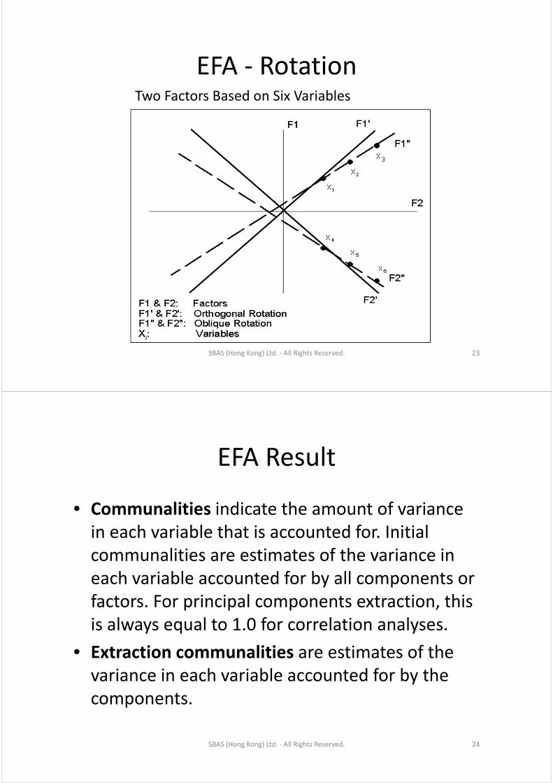
EFA RotationEFA ‐ RotationTwo Factors Based on Six Variables
SBAS (Hong Kong) Ltd. ‐ All Rights Reserved. 23
EFA ResultEFA Result
• Communalities indicate the amount of variance in each variable that is accounted for. Initial communalities are estimates of the variance in each variable accounted for by all components or y pfactors. For principal components extraction, this is always equal to 1.0 for correlation analyses.is always equal to 1.0 for correlation analyses.
• Extraction communalities are estimates of the variance in each variable accounted for by thevariance in each variable accounted for by the components.
SBAS (Hong Kong) Ltd. ‐ All Rights Reserved. 24
EFA ResultEFA Result (cont’d)
F h i i i l l i f T l V i E l i d• For the initial solution of Total Variance Explained, there are as many components as variables, and in a correlations analysis the sum of the eigenvalues equalscorrelations analysis, the sum of the eigenvalues equals the number of components. Extracted those components with eigenvalues greater than 1.p g g
• The rotated component matrix helps you to determine what the components represent.p p
• For each case and each component, the component score is computed by multiplying the case's standardized variable values (computed using listwisedeletion) by the component's score coefficients.
SBAS (Hong Kong) Ltd. ‐ All Rights Reserved. 25
Exploratory Factor Analysis
• Demo
• Q&A
SBAS (Hong Kong) Ltd. ‐ All Rights Reserved. 26
Confirmatory Factor AnalysisConfirmatory Factor Analysis
• Test whether measures of a construct are consistent with a researcher's understanding gof the nature of that construct (or factor). As such the objective of confirmatory factorsuch, the objective of confirmatory factor analysis is to test whether the data fit a hypothesized measurement model Thishypothesized measurement model. This hypothesized model is based on theory and/or previous analytic research
SBAS (Hong Kong) Ltd. ‐ All Rights Reserved. 27
Difference between EFA and CFADifference between EFA and CFA
• Both exploratory factor analysis (EFA) and confirmatory factor analysis (CFA) are y y ( )employed to understand shared variance of measured variables that is believed to bemeasured variables that is believed to be attributable to a factor or latent construct. Despite this similarity however EFA and CFADespite this similarity, however, EFA and CFA are conceptually and statistically distinct analyses.
SBAS (Hong Kong) Ltd. ‐ All Rights Reserved. 28

Difference between EFA and CFA ( ’d)Difference between EFA and CFA (cont’d)
Th l f EFA i id if f b d d d• The goal of EFA is to identify factors based on data and to maximize the amount of variance explained. The researcher is not required to have any specificresearcher is not required to have any specific hypotheses about how many factors will emerge, and what items or variables these factors will comprise.p
• By contrast, CFA evaluates a priori hypotheses and is largely driven by theory. CFA analyses require the g y y y y qresearcher to hypothesize, in advance, the number of factors, whether or not these factors are correlated, d hi h it / l d t d fl t hi hand which items/measures load onto and reflect which
factors.
SBAS (Hong Kong) Ltd. ‐ All Rights Reserved. 29
CFA and SEMCFA and SEM
St t l ti d li ft i t i ll d• Structural equation modeling software is typically used for performing confirmatory factor analysis. CFA is also frequently used as a first step to assess the proposed q y p p pmeasurement model in a structural equation model. Many of the rules of interpretation regarding assessment of model fit and model modification inassessment of model fit and model modification in SEM apply equally to CFA. CFA is distinguished from structural equation modeling by the fact that in CFA, there are no directed arrows between latent factors. In the context of SEM, the CFA is often called 'the measurement model' while the relations between themeasurement model , while the relations between the latent variables (with directed arrows) are called 'the structural model'.
SBAS (Hong Kong) Ltd. ‐ All Rights Reserved. 30
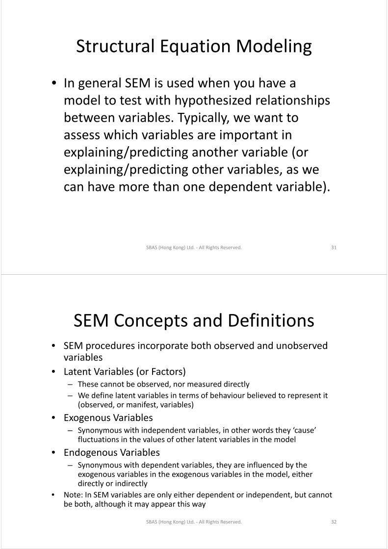
Structural Equation ModelingStructural Equation Modeling
• In general SEM is used when you have a model to test with hypothesized relationships yp pbetween variables. Typically, we want to assess which variables are important inassess which variables are important in explaining/predicting another variable (or explaining/predicting other variables as weexplaining/predicting other variables, as we can have more than one dependent variable).
SBAS (Hong Kong) Ltd. ‐ All Rights Reserved. 31
SEM Concepts and DefinitionsSEM Concepts and Definitions• SEM procedures incorporate both observed and unobserved p p
variables
• Latent Variables (or Factors)h b b d d d l– These cannot be observed, nor measured directly
– We define latent variables in terms of behaviour believed to represent it (observed, or manifest, variables)
• Exogenous Variables– Synonymous with independent variables, in other words they ‘cause’
fluctuations in the values of other latent variables in the modelfluctuations in the values of other latent variables in the model
• Endogenous Variables– Synonymous with dependent variables, they are influenced by the
i bl i th i bl i th d l ithexogenous variables in the exogenous variables in the model, either directly or indirectly
• Note: In SEM variables are only either dependent or independent, but cannot be both altho gh it ma appear this abe both, although it may appear this way
SBAS (Hong Kong) Ltd. ‐ All Rights Reserved. 32
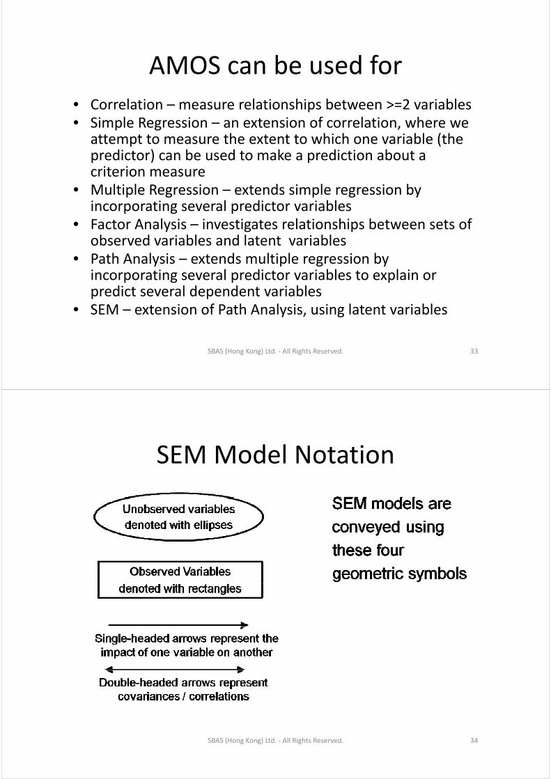
AMOS can be used forAMOS can be used for
• Correlation – measure relationships between >=2 variablesCorrelation measure relationships between > 2 variables• Simple Regression – an extension of correlation, where we
attempt to measure the extent to which one variable (the di t ) b d t k di ti b tpredictor) can be used to make a prediction about a
criterion measure• Multiple Regression – extends simple regression byMultiple Regression extends simple regression by
incorporating several predictor variables• Factor Analysis – investigates relationships between sets of
b d i bl d l t t i blobserved variables and latent variables• Path Analysis – extends multiple regression by
incorporating several predictor variables to explain or p g p ppredict several dependent variables
• SEM – extension of Path Analysis, using latent variables
SBAS (Hong Kong) Ltd. ‐ All Rights Reserved. 33
SEM Model NotationSEM Model Notation
SBAS (Hong Kong) Ltd. ‐ All Rights Reserved. 34
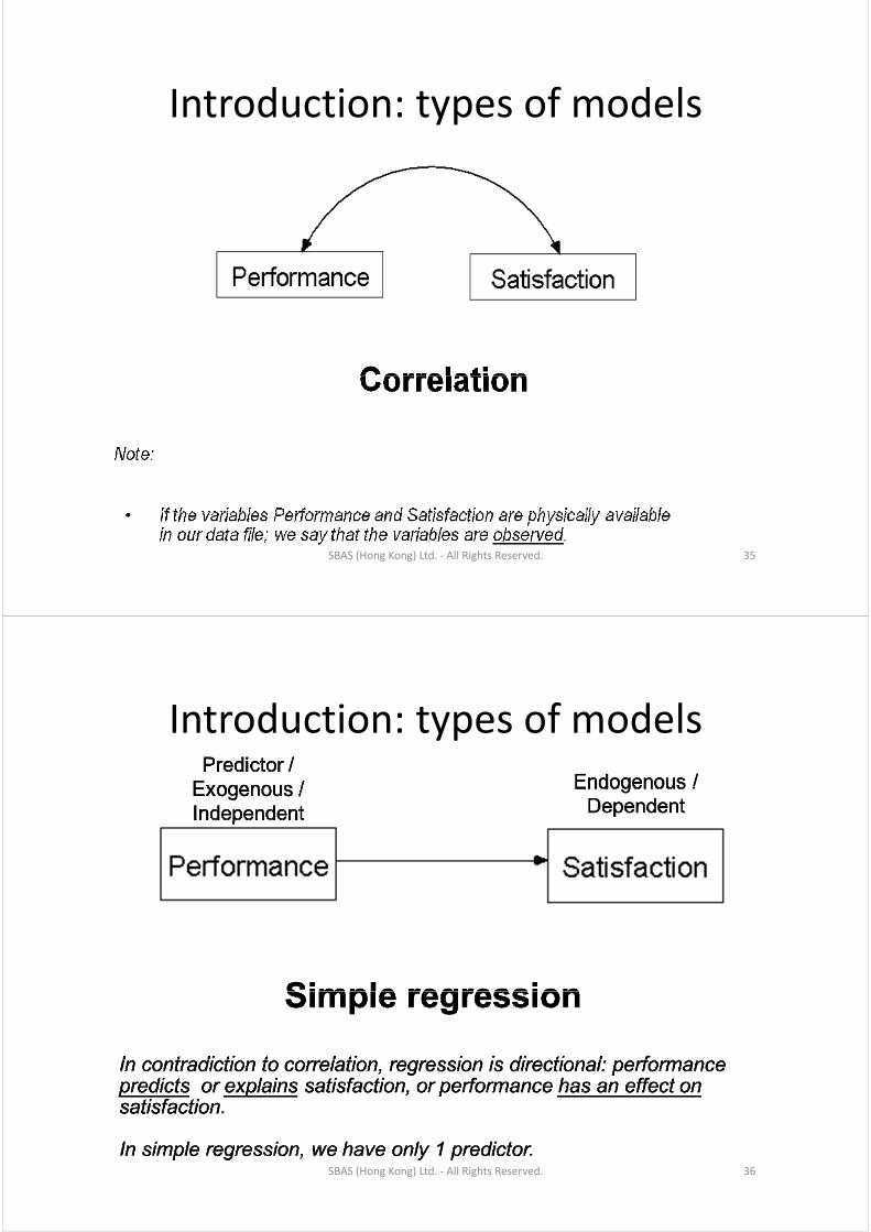
Introduction: types of modelsIntroduction: types of models
SBAS (Hong Kong) Ltd. ‐ All Rights Reserved. 35
Introduction: types of modelsIntroduction: types of models
SBAS (Hong Kong) Ltd. ‐ All Rights Reserved. 36
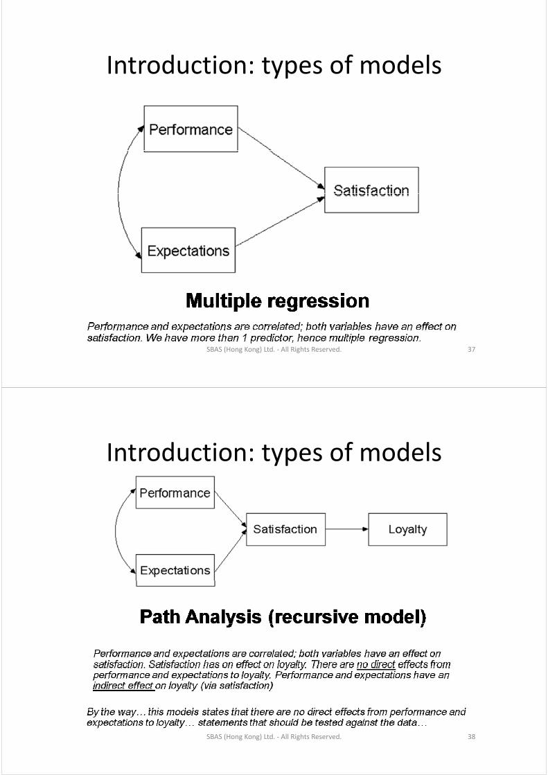
Introduction: types of modelsIntroduction: types of models
SBAS (Hong Kong) Ltd. ‐ All Rights Reserved. 37
Introduction: types of modelsIntroduction: types of models
SBAS (Hong Kong) Ltd. ‐ All Rights Reserved. 38
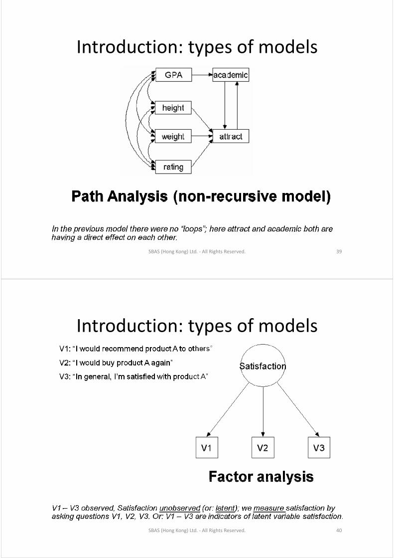
Introduction: types of modelsIntroduction: types of models
SBAS (Hong Kong) Ltd. ‐ All Rights Reserved. 39
Introduction: types of modelsIntroduction: types of models
SBAS (Hong Kong) Ltd. ‐ All Rights Reserved. 40
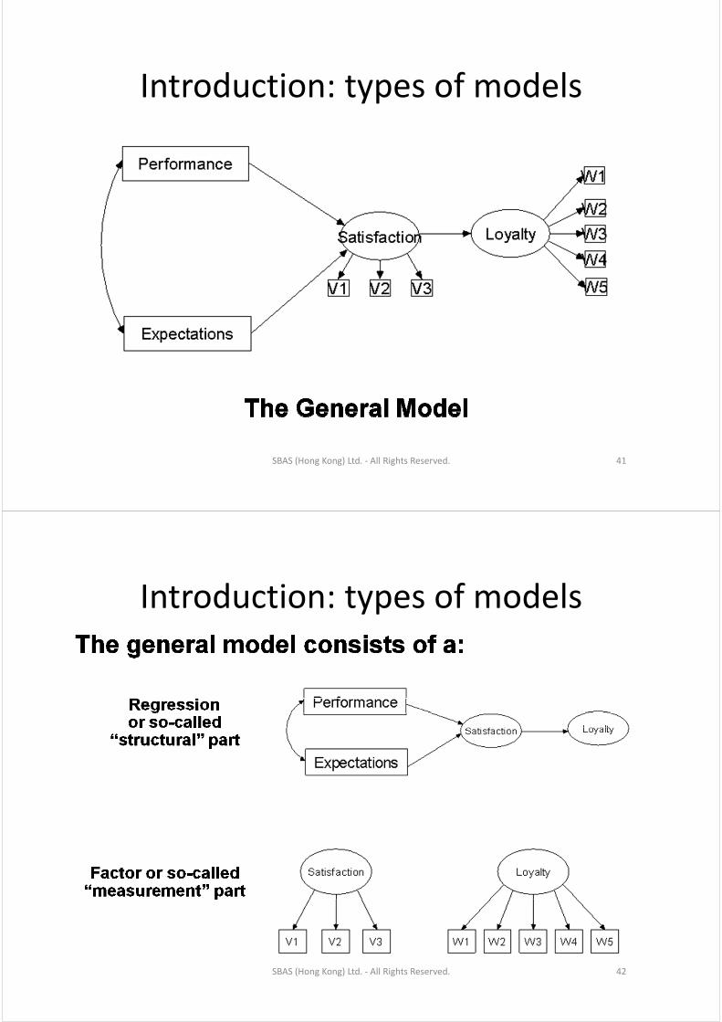
Introduction: types of modelsIntroduction: types of models
SBAS (Hong Kong) Ltd. ‐ All Rights Reserved. 41
Introduction: types of modelsIntroduction: types of models
SBAS (Hong Kong) Ltd. ‐ All Rights Reserved. 42
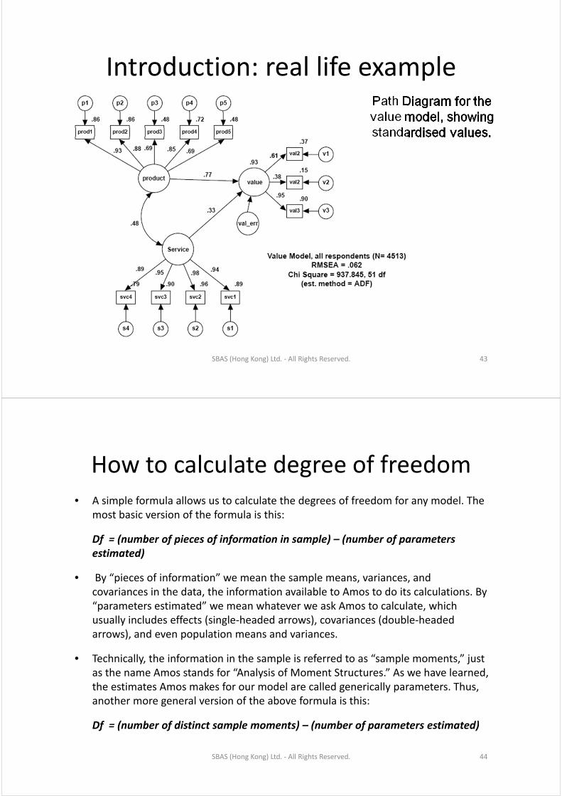
Introduction: real life exampleIntroduction: real life example
SBAS (Hong Kong) Ltd. ‐ All Rights Reserved. 43
How to calculate degree of freedomHow to calculate degree of freedom• A simple formula allows us to calculate the degrees of freedom for any model. The
most basic version of the formula is this:
Df = (number of pieces of information in sample) – (number of parameters estimated)estimated)
• By “pieces of information” we mean the sample means, variances, and covariances in the data, the information available to Amos to do its calculations. By , y“parameters estimated” we mean whatever we ask Amos to calculate, which usually includes effects (single‐headed arrows), covariances (double‐headed arrows), and even population means and variances.
• Technically, the information in the sample is referred to as “sample moments,” just as the name Amos stands for “Analysis of Moment Structures.” As we have learned, th ti t A k f d l ll d i ll t Ththe estimates Amos makes for our model are called generically parameters. Thus, another more general version of the above formula is this:
Df = (number of distinct sample moments) – (number of parameters estimated)Df (number of distinct sample moments) (number of parameters estimated)
SBAS (Hong Kong) Ltd. ‐ All Rights Reserved. 44
How to calculate degree of freedom ( t’d)How to calculate degree of freedom (cont’d)
• Number of distinct sample moment
= p * (p+1) / 2, where p is the number of p (p+1) / 2, where p is the number of observed variables
• Number of parameters estimatedp
= direct effects + variances + covariances
SBAS (Hong Kong) Ltd. ‐ All Rights Reserved. 45
Amos how to operateAmos – how to operate
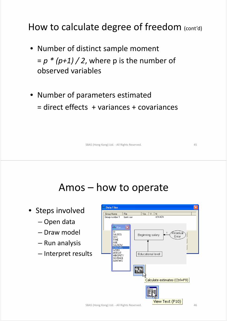
• Steps involved
– Open dataOpen data
– Draw model
R l i– Run analysis
– Interpret results
SBAS (Hong Kong) Ltd. ‐ All Rights Reserved. 46
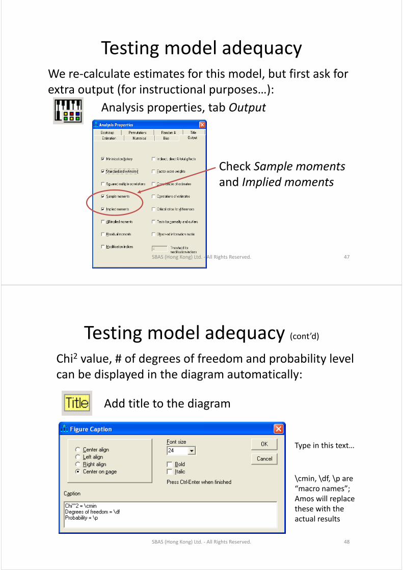
Testing model adequacyTesting model adequacyWe re‐calculate estimates for this model, but first ask for ,extra output (for instructional purposes…):
Analysis properties, tab OutputAnalysis properties, tab Output
Check Sample momentsand Implied moments
SBAS (Hong Kong) Ltd. ‐ All Rights Reserved. 47
Testing model adequacyTesting model adequacy (cont’d)Chi2 value, # of degrees of freedom and probability level , g p ycan be displayed in the diagram automatically:
Add title to the diagram
Type in this text…
\cmin, \df, \p are “macro names”;macro names ; Amos will replace these with the actual results
SBAS (Hong Kong) Ltd. ‐ All Rights Reserved. 48
Testing model adequacyTesting model adequacy (cont’d)
E d l i li ifi ( l i ) l i• Every model implies specific (population) correlations between the variables, so every model implies a certain population correlation matrix.p p
• The model is our null hypothesis.
• On the other hand we have the observed correlations, so we have a sample correlation matrix
• A Chi2 test is used to asses the discrepancy between these two matricesa If probability < 0 05 we reject our model; iftwo matricesa. If probability < 0.05, we reject our model; if probability >= 0.05, we do not reject our model
– aTechnical note: actually the discrepancy between the sample variance/covariance matrix and the implied variance/covariance matrix is used in the Chi2 test, not the correlation matrix,
SBAS (Hong Kong) Ltd. ‐ All Rights Reserved. 49
Testing model adequacyTesting model adequacy (cont’d)• In traditional testing we (as the researcher) have a certain hypothesis we want to “prove” by trying to reject a null hypothesis which states the contrary. We stick to this null‐hypothesis until it’s very unlikely, in which case we accept our own hypothesis.
• Here, the null hypothesis has the benefit of the doubt.
• In SEM we (as the researcher) postulate a model and we believe in this model (and nothing but the model),we believe in this model (and nothing but the model), until this model appears to be unlikely.
• Now we (our model) has the benefit of the doubt• Now, we (our model) has the benefit of the doubt.
SBAS (Hong Kong) Ltd. ‐ All Rights Reserved. 50

How to correct a modelHow to correct a model
Analysis Properties tab OutputAnalysis Properties, tab Output
Ch k thi tiCheck this option (note: that by default the threshold is 4; if the MI for athreshold is 4; if the MI for a particular restriction < 4, then it will not be reported in the output)
SBAS (Hong Kong) Ltd. ‐ All Rights Reserved. 51
Multiple Group AnalysisMultiple Group Analysis
• We run a multiple group analysis when we want to test whether a particular model holds pfor each and every group within our dataset
• In other words we are testing to see if there is• In other words, we are testing to see if there is an interaction effect: is the model group‐dependent?
SBAS (Hong Kong) Ltd. ‐ All Rights Reserved. 52
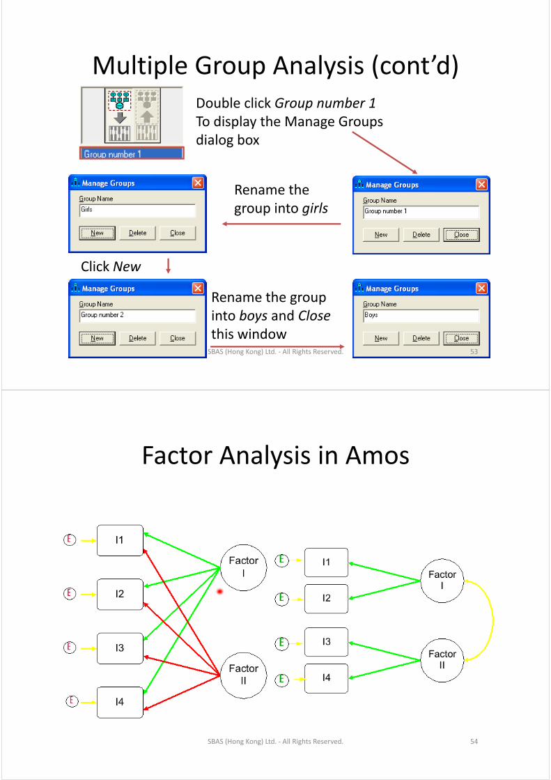
Multiple Group Analysis (cont’d)Multiple Group Analysis (cont d)Double click Group number 1pTo display the Manage Groups dialog box
Rename the group into girls
Click New
Rename the group into boys and Close this windowSBAS (Hong Kong) Ltd. ‐ All Rights Reserved. 53
Factor Analysis in AmosFactor Analysis in Amos
SBAS (Hong Kong) Ltd. ‐ All Rights Reserved. 54
Factor Analysis in AmosFactor Analysis in Amos (cont’d)
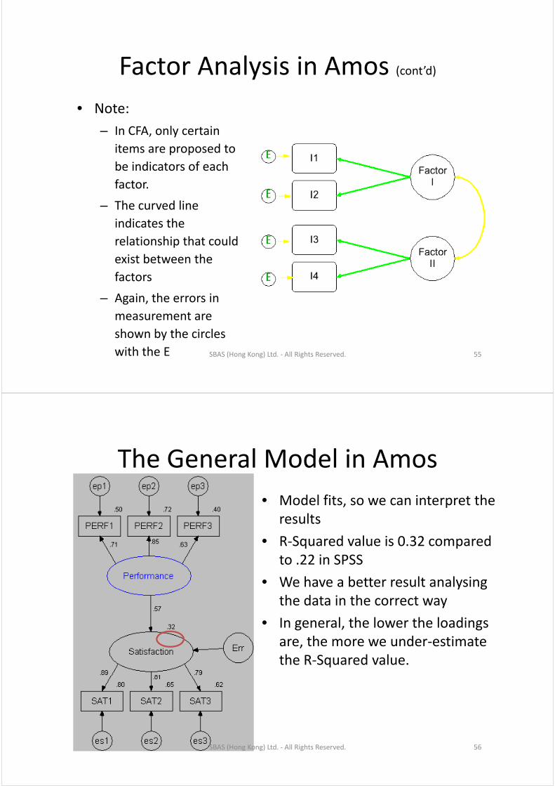
• Note:• Note:
– In CFA, only certain
items are proposed toitems are proposed to
be indicators of each
factor.
– The curved line
indicates the
relationship that couldrelationship that could
exist between the
factors
– Again, the errors in
measurement are
shown by the circles
with the E SBAS (Hong Kong) Ltd. ‐ All Rights Reserved. 55
The General Model in AmosThe General Model in Amos
• Model fits so we can interpret theModel fits, so we can interpret the results
• R‐Squared value is 0.32 comparedR Squared value is 0.32 compared to .22 in SPSS
• We have a better result analysing y gthe data in the correct way
• In general, the lower the loadings are, the more we under‐estimate the R‐Squared value.
SBAS (Hong Kong) Ltd. ‐ All Rights Reserved. 56
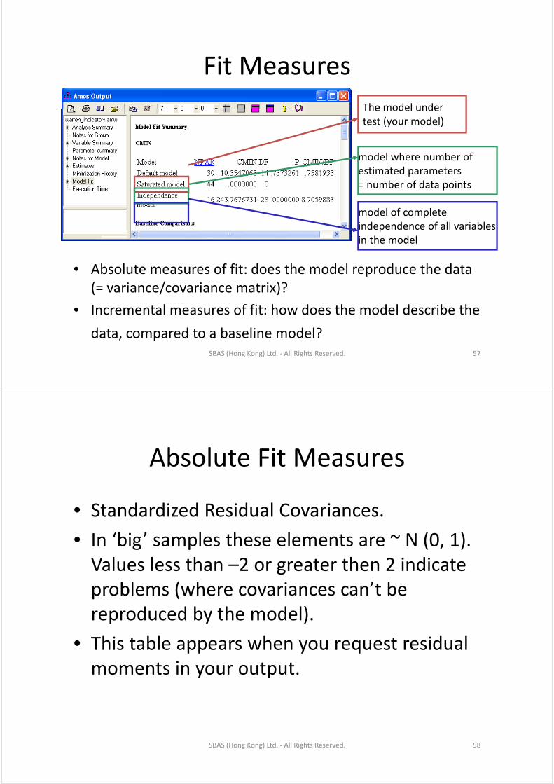
Fit MeasuresFit Measures
The model underThe model undertest (your model)
model where number of estimated parameters= number of data points
model of complete independence of all variables in the model
• Absolute measures of fit: does the model reproduce the data ( i / i i )?
in the model
(= variance/covariance matrix)?
• Incremental measures of fit: how does the model describe the
data, compared to a baseline model?SBAS (Hong Kong) Ltd. ‐ All Rights Reserved. 57
Absolute Fit MeasuresAbsolute Fit Measures
• Standardized Residual Covariances.
• In ‘big’ samples these elements are ~ N (0, 1).In big samples these elements are N (0, 1). Values less than –2 or greater then 2 indicate problems (where covariances can’t beproblems (where covariances can t be reproduced by the model).
• This table appears when you request residual moments in your output.moments in your output.
SBAS (Hong Kong) Ltd. ‐ All Rights Reserved. 58
Absolute Fit MeasuresAbsolute Fit Measures (cont’d)
Chi2/df (Wh t M thé Al i & S• Chi2/df (Wheaton,Muthén, Alwin & Summers 1977)
• Problem distribution of this statistic does not• Problem: distribution of this statistic does not exist, so people have rules of thumb:
• Wheaton (1977) Chi2 / df <= 5 is acceptable fit• Wheaton (1977) Chi2 / df <= 5 is acceptable fit.• Carmines: Chi2 / df <= 3 is acceptable fitB (1989) “it l th t ti > 2 00• Byrne (1989): “it seems clear that a ratio > 2.00 represents an inadequate fit.”
• Amos User Guide: ‘close to 1 for correct models’• Amos User Guide: close to 1 for correct models• Note: Wheaton (1987) later advocated that this ratio not be used
SBAS (Hong Kong) Ltd. ‐ All Rights Reserved. 59
Absolute Fit MeasuresAbsolute Fit Measures (cont’d)
P l ti di• Population discrepancy.– Idea: how far is Chi2 value from expected value? This difference divided by sample size (labelled F0)difference divided by sample size (labelled F0).
• Root Mean Square Error of Approximation– Browne et al: ‘RMSEA of 0 05 or less indicates a closeBrowne et al: RMSEA of 0.05 or less indicates a close fit’
– It can be tested: H0: “RMSEA <= 0.05” (compare with regular Chi2 test: “RMSEA = 0”)
– Amos gives this probability (H0: RMSEA <= 0.05) in Pclose In words: Pclose is the probability that thePclose. In words: Pclose is the probability that the model is almost correct.
SBAS (Hong Kong) Ltd. ‐ All Rights Reserved. 60
Relative Fit MeasuresRelative Fit Measures
NFI N d Fit I d (B tl & B tt’ 1980)• NFI – Normed Fit Index (Bentler & Bonnett’s 1980)– was the practical criterion of choice for several yearsAddressing evidence that the NFI has shown a– Addressing evidence that the NFI has shown a tendency to underestimate fit in small samples, Bentler revised this measure, taking in to account sample size – the CFI, Comparative Fit Index
– Both range from 0 to 1V l f 9 i i ll d ll fitti– Value of >.9 was originally proposed as well‐fitting model
– Revised value of > 95 advised by Hu &Bentler (1999)Revised value of >.95 advised by Hu &Bentler (1999)
– Note: Bentler (1980) suggested CFI was measure of choice
SBAS (Hong Kong) Ltd. ‐ All Rights Reserved. 61
Relative Fit MeasuresRelative Fit Measures (cont’d)
RFI R l ti Fit I d• RFI – Relative Fit Index– Derivative of NFIRange of values from 0 to 1 with values close to 0 95– Range of values from 0 to 1, with values close to 0.95 indicating superior fit (Hu & Bentler 1999)
• IFI – Incremental Index of FitIFI Incremental Index of Fit– Issues of parsimony and sample size with NFI lead to Bollen (1989) develop this measure
– Same calculation as NFI, but degrees of freedom taken into accountA i l f 0 t 1 ith th l t– Again values range from 0 to 1, with those close to 0.95 indicating well‐fitting models
SBAS (Hong Kong) Ltd. ‐ All Rights Reserved. 62
Relative Fit MeasuresRelative Fit Measures (cont’d)
GFI G d f Fit I d• GFI – Goodness of Fit Index– A measures of the relative amount of variance & covariance in the sample covariance matrix (ofcovariance in the sample covariance matrix (of observed variables) that is jointly explained by the population matrix
– Values range from 0 to 1 (though –ve value theoretically possible) with 1 being the perfect model of fit. Rule of thumb is either >.8 or >.9of fit. Rule of thumb is either >.8 or >.9
• AGFI – Adjusted Goodness of Fit Index– Correction of GFI to include degrees of freedomCorrection of GFI to include degrees of freedom– Values interpreted as above
SBAS (Hong Kong) Ltd. ‐ All Rights Reserved. 63
Relative Fit MeasuresRelative Fit Measures (cont’d)
• PGFI – Parsimony Goodness of Fit Index
– Takes into account the complexity (i.e. number of p y (estimated parameters)
– Provides more realistic evaluation of the modelProvides more realistic evaluation of the model (Mulaik et al, 1989
Typically parsimony fit indices have lower– Typically parsimony fit indices have lower thresholds, so values in the .50’s are not uncommon and can accompany other indices inuncommon, and can accompany other indices in the .90’s
SBAS (Hong Kong) Ltd. ‐ All Rights Reserved. 64
Other Fit MeasuresOther Fit Measures
AIC Ak ik ’ I f i C i i d CAIC• AIC ‐ Akaike’s Information Criteria and CAIC –Consistent Akaike’s Information Criteria
Both address the issue of parsimony and goodness of fit– Both address the issue of parsimony and goodness of fit, but AIC only relates to degrees of freedom. Bozdogan(1987) proposed CAIC to take into account sample size
– Used in the comparison of 2 or more models, with smaller values representing a better fit of the model
• BIC (Bayes Information Criterion) and BCC (Browne‐Cudeck Criterion)
O i h AIC d CAIC b i– Operate in the same way as AIC and CAIC, but impose greater penalties for model complexity
SBAS (Hong Kong) Ltd. ‐ All Rights Reserved. 65
Other Fit MeasuresOther Fit Measures (cont’d)
H lt ’ C iti l N• Hoelter’s Critical N:– Last goodness of fit statistic appearing in the Amos outputoutput
– In fact two values for levels of significance of .05 and .01
– Differs substantially from those previously mentioned– Focuses directly on sample size, rather than model fit– It’s purpose is to estimate a sample size that would be sufficient to yield an adequate model fit for a χ2 testHoelter proposed a value > 200 is indicative of a– Hoelter proposed a value > 200 is indicative of a model that adequately represents the sample data
SBAS (Hong Kong) Ltd. ‐ All Rights Reserved. 66

AMOS (CFA and SEM)
• Demo
• Q&A
SBAS (Hong Kong) Ltd. ‐ All Rights Reserved. 67SBAS (Hong Kong) Ltd. ‐ All Rights Reserved. 67