Northern High-latitude Climate Response to Mid-Holocene Insolation: Model-data Comparisons

Qiong Zhang, Hanna Sundqvist

The Bert Bolin Centre for Climate ResearchStockholm University, Sweden

With contributions of

Anders Moberg, Karin Holmgren

(Department of Physical Geography and Quaternary )

Erland Källén, Heiner Körnich and Johann Nilsson

(Department of Meteorology)

Christophe Sturm

(Department of Geological Sciences)

BBCC project: Holocene climate variability over Scandinavia

1. A number of reconstructions are available for Holocene over highlatitudes.

2. The mid-Holocene is a key period of interest for the Palaeoclimate Modeling Intercomparison Project (PMIP), the different types of model simulations are available for studying.

3. To increase the understanding of the climate change of the mid-Holocene through integrating proxy data analysis and global climate modelling.

Holocene temperature changes

IPCC AR4IPCC AR4

Outline

1 Evidence of 6 ka climate change in reconstructions

2 Climate response in PMIP1 and PMIP2

3 Model-data comparison with an optimal selection method

4 The feedback mechanism

5 Application of stable water isotope modeling in palaeoclimate

Climate reconstructions from proxy data

Number of reconstructions: 72Number of sites: 61

Summer temperature: 48Winter temperature: 7Annual mean temperature: 16

The collected reconstructions have records both in

mid-Holocene (~6000yrs BP) and pre-industrial (~1750)

pollen diatoms chironomids

speleothemsIce-coresborehole

diatoms alkenones foraminifera

Type of proxy data used

Terrestrial, 65Pollen, 40

Chironomids, 12

Diatoms, 6

Borehole, 2

Ice-cores, 1

Tree-rings, 1

Speleothems, 2

Density of sediment, 1

Marine, 7Foraminifera, 3Diatoms, 2Alkenones, 1Dinocysts, 1

Uncertainty of the reconstructions

1. Statistical calibration uncertainty,σc

2. Internal variability uncertainty, σv

σcom2= σc

2+σv2

Calibration error σc

The frequency distribution of calibration σcand internal variability σv

Temperature change in reconstructions (6ka-0ka)

Averaged difference 2.1 C±0.72 C

Averaged difference 1.8 C±1.7 C

Averaged difference 1.0 C±0.96 C

Annual mean T(16 data) Summer T(48 data) Winter T(6 data)

Motivation of PMIP

� Study the role of climate feedbacks� Atmosphere --------PMIP1 � Ocean, sea-ice-----PMIP2-OA� Vegetation-----------PMIP2-OAV

� Model evaluation� Testing climate models

� Model-model comparison� Model-data comparison

� Key periods:� LGM (21 ka)� Mid-Holocene (6ka)� Pre-industrial (0ka) ----Control run� Last Millennium (PMIP3)

6-10, December, 2010, Japan

Boundary Conditions for Mid-Holocene (6ka) and Pre-Industrial (0ka)

Ice sheets, topography, trace gases and Earth’s orbital parameters

Ice Sheets Topography Coastlines

CO2

(ppmv)

CH4

(ppbv)

NO2

(ppbv)

Eccentricity Obliquity(º) Angular precession(º)

0ka Modern Modern 280 760 270 0.0167724 23.446 102.04

6ka Same as 0k Same as 0k 280 650 270 0.018682 24.105 0.87

Change in incoming solar radiation at the top of the atmosphere(6Ka-0Ka)

Insolation forcing (Change between 6ka and 0ka)

The insolation change at Northern high latitude (60 N-90 N)

Summer : 23.5 W/m2

Winter : -2.3 W/m2

Annual : 2.9 W/m2

60-90 N average

PMIP models used in comparisonPMIP1-Atmosphere only model, fixed SST

19 models:

bmrc,ccc2.0,ccm3,ccsr1,climber2,cnrm2,csiro,echam3,gen2,gfdl,

giss-iip,lmcelmd4,lmcelmd5,mri2,msu,ugamp,uiuc11,ukmo,yonu

10years simulation under the 6ka and 0ka boundary condition

PMIP2-OA: Atmosphere-ocean coupled model

13 models:CCSM,CSIRO_Mk3L-1.0,CSIRO-Mk3L-1.1,ECBILTCLIOVECODE,ECHAM5-MPIOM1,FGOALS-1.0g,FOAM,GISSmodelE,IPSL-CM4-V1-MR,MIROC3.2,MRI-CGCM2.3.4fa,MRI-CGCM2.3.4nfa,UBRIS-HadCM3M2

100years simulation under the 6ka and 0ka boundary condition

PMIP2-OAV: Atmosphere-ocean-vegetation coupled model

6 models:

ECBILTCLIOVECODE,ECHAM53-MPIOM1-LPJ,FOAM,MRI-CGCM2.3.4fa,MRI-CGCM2.3.4nfa,UBRIS-HadCM3M2

100years simulation under the 6ka and 0ka boundary condiction

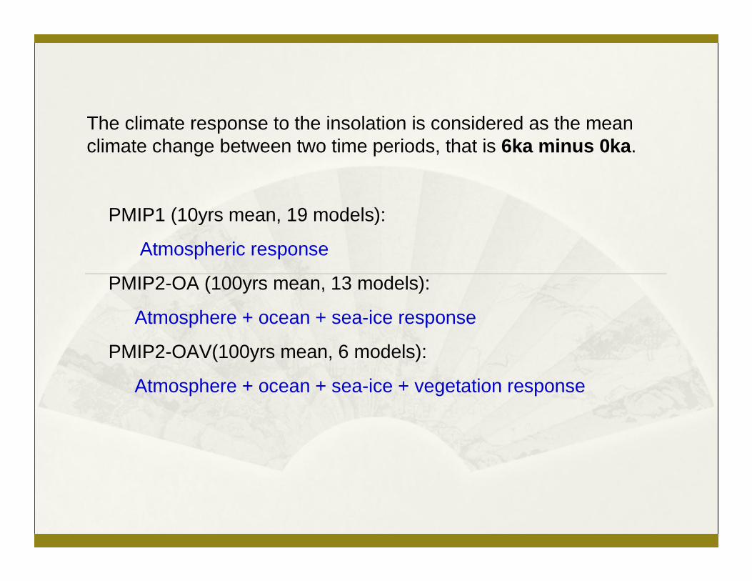
The climate response to the insolation is considered as the meanclimate change between two time periods, that is 6ka minus 0ka.

PMIP1 (10yrs mean, 19 models):

Atmospheric response

PMIP2-OA (100yrs mean, 13 models):

Atmosphere + ocean + sea-ice response

PMIP2-OAV(100yrs mean, 6 models):

Atmosphere + ocean + sea-ice + vegetation response

Annual temperature change in 3 types of PMIP models

PMIP1-SSTf1 = bmrc 11 = giss-iip2 = ccc2.0 12 = lmcelmd43 = ccm3 13 = lmcelmd5 4 = ccsr1 14 = mri25 = climber2 15 = msu6 = cnrm2 16 = ugamp7 = csiro 17 = uiuc118 = echam3 18 = ukmo9 = gen2 19 = yonu

10 = gfdl

PMIP2-OA1 = CCSM2 = CSIRO-Mk3L-1.03 = CSIRO-Mk3L-1.1 4 = ECBILTCLIOVECODE 5 = ECHAM5-MPIOM16 = FGOALS-1.0g7 = FOAM 8 = GISSmodelE9 = IPSL-CM4-V1-MR1

10 = MIROC3.211 = MRI-CGCM2.3.4fa12 = MRI-CGCM2.3.4nfa13 = UBRIS-HadCM3M2

PMIP2-OAV1 = ECBILTCLIOVECODE2 = ECHAM53-MPIOM1-LPJ3 = FOAM4 = MRI-CGCM2.3.4fa5 = MRI-CGCM2.3.4nfa6 = UBRIS-HadCM3M2

Models

- 0.03 0.64 1.70

Averaged over 60-90N

Seasonal temperature change in 3 types of PMIP modelsSpring (MAM)

-0.12

-0.51

-0.33

-0.46 0.22 0.84 1.13 1.50

Summer(JJA)

Autumn(SON) Winter(DJF)

1.220.551.35 2.18

Model ensemble and data Summer WinterAnnual mean

PMIP1-SSTf (19 simulations ensemble) 0.80 -0.01 0.02

PMIP2-OA (13 simulations ensemble) 1.13 0.35 0.42

PMIP2-OA (5 simulations ensemble ) 1.00 0.82 0.57

PMIP2-OAV(5 simulations ensemble) 1.22 1.17 0.81

Reconstructions 1.00 1.71 2.04

Seasonal changes in temperature (ºC) averaged over the locations of available reconstructions

Uncertainties across the climate model

Hugues Goosse et al, 2006

Model-data comparison: Selection of the optimal simulations

The ‘‘optimal’’ simulation for each PMIP2 is selected as the one that has the minimum of a cost function of:

11

2 +=

σiw

∑=

−=n

i

kiirecik FFwCF

1

2mod,, )(

Cost function for the PMIP ensemble

Model type Summer Winter Annual mean

w1 w2 w1 w2 w1 w2

PMIP1-SSTf 1.04 0.73 2.49 1.34 2.23 1.67

PMIP2-OA 1.05 0.77 2.26 1.17 1.87 1.39

PMIP2-OAV 1.06 0.77 1.95 0.88 1.59 1.20

11

22 +=

σwN

w 11 =

PMIP2-OA1 = CCSM2 = CSIRO-Mk3L-1.03 = CSIRO-Mk3L-1.1 4 = ECBILTCLIOVECODE 5 = ECHAM5-MPIOM16 = ECHAM53 LPJ7 = FGOALS-1.0g8 = FOAM 9 = GISSmodelE

10 = IPSL-CM4-V1-MR111 = MIROC3.212 = MRI-CGCM2.3.4fa13 = UBRIS-HadCM3M2

PMIP2-OAV1 = ECBILTCLIOVECODE2 = ECHAM53-MPIOM1-LPJ3 = FOAM4 = MRI-CGCM2.3.4fa5 = UBRIS-HadCM3M2

Cost function for the 18 PMIP2 models

Fig. 6. The large scale pattern in surface temperature(°C) change in FOAM-OA (left column), MRI CGCM2.3.4fa-OA (middle column), and reconstructions (right column). Top row is for summer temperature, represented by JJA mean for model data and July temperature for reconstructions; middle row is for winter temperature, represented by DJF mean for model data and January temperature for reconstructions; bottom row is for annual mean temperature.

The large scale pattern in surface temperature (ºC) change in FOAM-OA, MRI-OA, and reconstructions

Summer

Winter

Annual

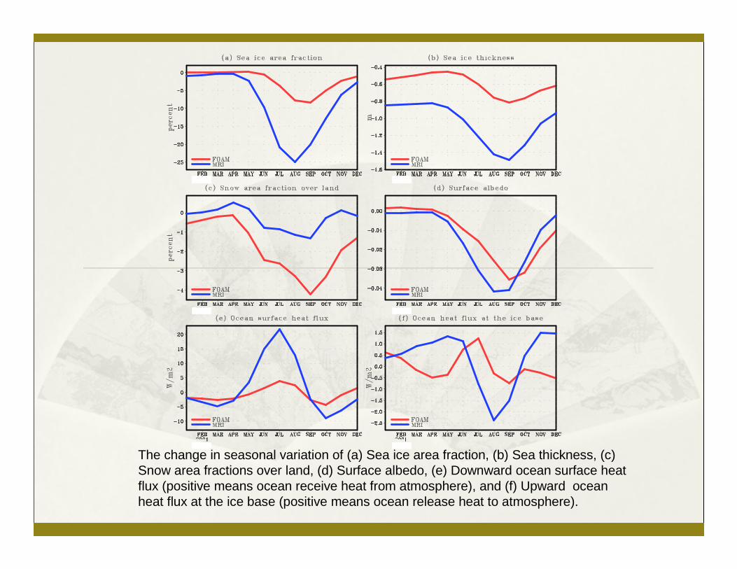
The change in seasonal variation of (a) Sea ice area fraction, (b) Sea thickness, (c) Snow area fractions over land, (d) Surface albedo, (e) Downward ocean surface heat flux (positive means ocean receive heat from atmosphere), and (f) Upward ocean heat flux at the ice base (positive means ocean release heat to atmosphere).

Change in Sea-ice coverage (%)

Change in Surface albedo and ocean surface heat flux

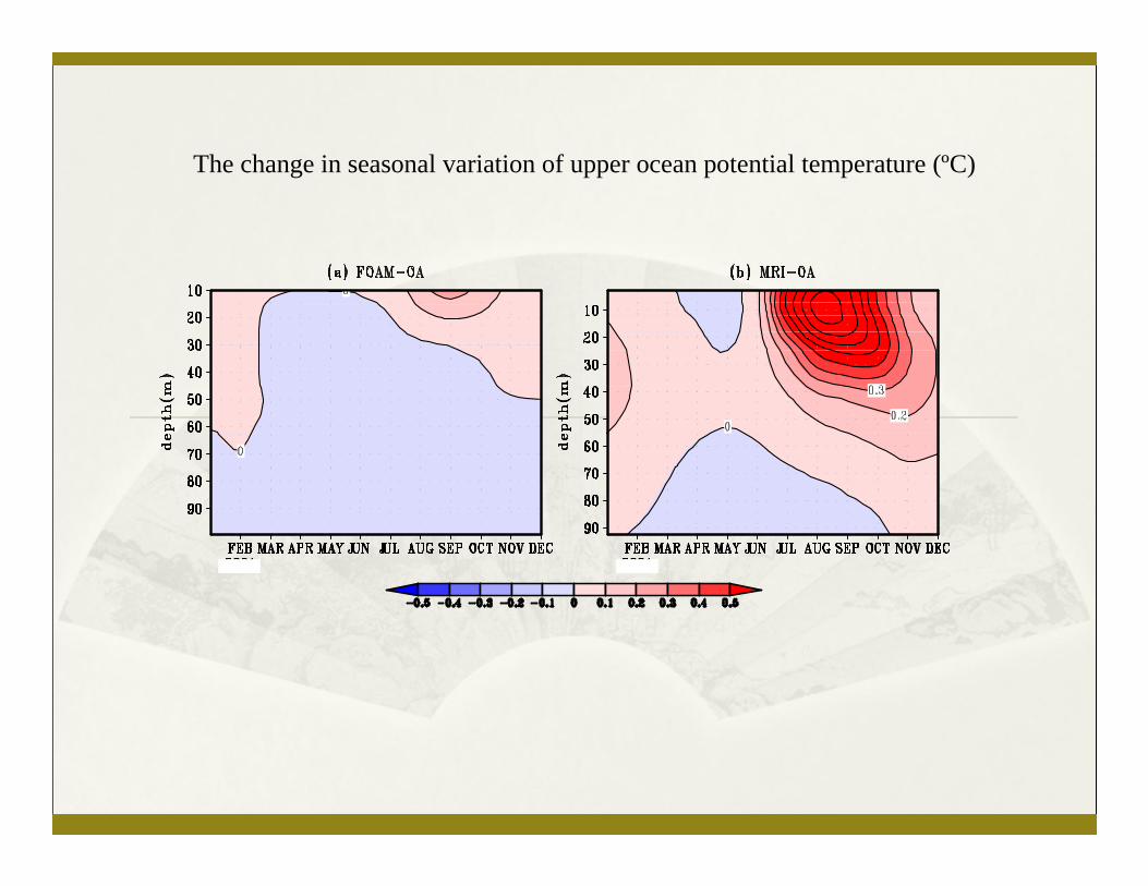
The change in seasonal variation of upper ocean potential temperature (ºC)

The change in DJF mean sea level pressure (Pa)

1. The reconstructions from different proxy data show 1.0 C warming in summer and 1.8 C warming in winter and 2.1 C warming in annual mean temperature over northern high latitudes.

2. Comparisons among 3 types of PMIP simulations indicate that whenmore physical feedbacks (ocean, sea-ice, vegetation) are included in the model, the climate response are better agree with the palaeoclimate records.

3. The optimal selected PMIP-OA models show that the summer warming in high latitude is enhanced by the sea-ice-albedo positive feedback. The response of the ocean and sea ice to the enhanced summer insolation further lead to a warming winter despite the reduced insolation.

Summary

Application of the stable water isotope modeling in palaeoclimate study

1. 18O-Temperture calibration ( 18O=0.67·Tsurf 13.6,Dansgaard,1964)2. Origin of the moisture

Model Institute References

CAM3 U. Colorado Noone et al., (2010)

CAM2 UC Berkeley Lee et al. (2007)

ECHAM5 AWI-Bremerhaven Werner et al., wip

ECHAM4 MPI-Hamburg Hoffmann et al (1998)

LMDZ4 LMD-Paris Risi et al., wip

MIROC3.2 JAMSTEC-Yokosuka Kurita et al. (2005)

GSM Scripps-San Diego Yoshimura et al. (2008)

GISS-E GISS-New York Schmidt et al (2007)

GENESIS Penn U. Mathieu et al (2002)

ACCESS ANSTO-Sydey Fischer et al., wip

HadCM3 U. Bristol Tindall et al. (2009)

HadAM3 BAS-Cambridge Sime et al. (2008)

Stable water isotope enabled GCM

Change in global annual mean temperature and 18O in CAM3-iso

Some climate response, such as the high latitude warming and North Africa cooling, also have the signatures in 18O..

Change in 18OChange in temperature

18O-T relationship over high latitudes from CAM3-iso

Sturm et al., 2010

Acknowledgement to Kei Yoshimura

Moisture origin with stable water isotope tracer

Model-data comparisons for high-latitude climate variability

Climate change: more collected data, and improved PMIP3 simulations

Climate variability:Challenge in data analysis:Different time resolution (10yr, 100yr), need downscaling or upscaling method to compile the collected reconstructions

Challenge in climate modelling: transient simulation

FOAM-LPJ: two transient simulations are available, 6500 yearsPMIP3 last millennium transient simulation

Outlook

Stable water isotope modellingRecent 140 year (1870-2009)Last millennium (Boundary condition from CESM1.0)

Related publications:

Sundqvist, H. S., Zhang, Q., Moberg, A., Holmgren, K., Körnich, H., Nilsson, J., and Brattström, G., 2010: Climate change between the mid and late Holocene in northern high latitudes – Part 1: Survey of temperature and precipitation proxy data, Clim. Past, 6, 591-608.

Zhang, Q., Sundqvist, H. S., Moberg, A., Körnich, H., Nilsson, J., and Holmgren, K., 2010: Climate change between the mid and late Holocene in northern high latitudes – Part 2: Model-data comparisons, Clim. Past, 6, 609-626.

Sturm, C., Zhang, Q., and Noone, D., 2010: An introduction to stable water isotopes in climate models: benefits of forward proxy modelling for paleoclimatology, Clim. Past, 6, 115-129.