prefixspan,: mining sequential patterns efficiently by

Prefixspan,: Mining Sequential Patterns Efficiently by Prefix-Projected Pattern Growth *

Jian Pei Jiawei Han Behzad Mortazavi-As1 Helen Pinto Intelligent Database Systems Research Lab. School of Computing Science, Simon Fraser University

Burnaby, B.C., Canada V5A 1 S6 E-mail: {peijian, han, mortazav, hlpinto} @cs.sfu.ca Qiming Chen Umeshwar Dayal Mei-Chun Hsu

Hewlett-Packard Labs. Palo Alto, California 94303-0969 U.S.A. E-mail: { qchen, dayal, mchsu} @hpl.hp.com

Abstract

Sequential pattern mining is an important data mining problem with broad applications. I t is challenging since one may need to examine a combinatorially explo- sive number of possible subsequence patterns. Most of the previously developed sequential pattern mining methods follow the methodology of A priori which may substantially reduce the number of combinations to be examined. How- eve6 Apriori still encounters problems when a sequence database is large andor when sequential patterns to be mined are numerous an&or long.

In this papel; we propose a novel sequential pattern mining method, called Prefixspan (i.e., Prefix-projected - Sequential Ettern_ mining), which explores prejx- projection in sequential pattern mining. Prefixspan mines the complete set of patterns but greatly reduces the efforts of candidate subsequence generation. Moreover; prefi-projection substantially reduces the size of projected databases and leads to efJicient processing. Our performance study shows that Prefixspan outperforms both the Apriori-based GSP algorithm and another recently proposed method; Frees pan, in mining large sequence data bases.

1 Introduction

Sequential pattern mining, which discovers frequent subsequences as patterns in a sequence database, is an important data mining problem with broad applications, in- cluding the analyses of customer purchase behavior, Web access patterns, scientific experiments, disease treatments, natural disasters, DNA sequences, and so on.

*The work was supported in part by the Natural Sciences and En- gineering Research Council of Canada (grant NSERC-A3723), the Net- works of Centres of Excellence of Canada (grant NCWIRIS-3). and the Hewlett-Packard Lab, U.S.A.

The sequential pattern mining problem was first intro- duced by Agrawal and Srikant in [2]: Given a set of sequences, where each sequence consists of a list of elements and each element consists of a set of items, and given a user-spec$ed minsupport threshold, sequential pattern mining is t o j n d all of the frequent subsequences, i.e., the subsequences whose occurrence frequency in the set of sequences is no less than minsupport.

Many studies have contributed to the efficient mining of sequential patterns or other frequent patterns in time- related data, e.g., [2, 11, 9, 10, 3, 8, 5, 41. Almost all of the previously proposed methods for mining sequential patterns and other time-related frequent patterns are Apriori-like, i.e., based on the Apriori property proposed in association mining [l] , which states the fact that any super-pattern of a nonfrequent pattern cannot be frequent.

Based on this heuristic, a typical Apriori-like method such as GSP [ 113 adopts a multiple-pass, candidate- generation-and-test approach in sequential pattern mining. This is outlined as follows. The first scan finds all of the frequent items which form the set of single item frequent sequences. Each subsequent pass starts with a seed set of sequential patterns, which is the set of sequential patterns found in the previous pass. This seed set is used to generate new potential patterns, called candidate sequences. Each candidate sequence contains one more item than a seed sequential pattern, where each element in the pattern may contain one or multiple items. The number of items in a sequence is called the length of the sequence. So, all the candidate sequences in a pass will have the same length. The scan of the database in one pass finds the support for each candidate sequence. All of the candidates whose support in the database is no less than minsupport form the set of the newly found sequential patterns. This set then becomes the seed set for the next pass. The algorithm terminates when no new sequential pattern is found in a pass, or no candidate sequence can be generated.

Similar to the analysis of Apriori frequent pattern min-

1063-6382/01$10.00 0 2001 IEEE 215

mailto:hpl.hp.com

ing method in [7], one can observe that the Apriori-like sequential pattern mining method, though reduces search space, bears three nontrivial, inherent costs which are in- dependent of detailed implementation techniques.

Potentially huge set of candidate sequences. Since the set of candidate sequences includes all the possible permutations of the elements and repetition of items in a sequence, the Apriori-based method may generate a really large set of candidate sequences even for a moderate seed set. For example, if there are 1000 frequent sequences of length-I, such as (al) , ( a z ) , . . . , (alooo), an Apriori-like algorithm will generate 1000 x 1000+- = 1,499,500 candidate sequences, where the first term is derived from the set (alal) , ( O l U Z ) , . . . , (alalooo), ( W l ) . (azaz), . . ., (u~ooou1ooo). and the second term is derived from the set ((alaz)), ((ala3)), . . . , ( ( ~ w ~ ~ I o o o ) ) . Multiple scans of databases. Since the length of each candidate sequence grows by one at each database scan, to find a sequential pattern { (abc)(ubc)(abc)(abc)(ubc)}, the Apriori-based method must scan the database at least 15 times. Difficulties at mining long sequential patterns. A long sequential pattern must grow from a combination of short ones, but the number of such candidate sequences is exponential to the length of the sequential patterns to be mined. For example, suppose there is only a single sequence of length 100, ( a l a2 . . .aloe), in the database, and the minsupport threshold is 1 (i.e., every occurring pattern is frequent), to (re-)derive this length- 100 sequential pattern, the Apriori-based method has to generate 100 length-1 candidate sequences, 100 x 100 + U!WB = 14,950 length-2 candidate sequences, (If) =

161,700 length-3 candidate sequences', . . . . Obvi- ously, the total number of candidate sequences to be generated is greater than 1030.

In many applications, it is not unusual that one may en- counter a large number of sequential patterns and long sequences, such as in DNA analysis or stock sequence analysis. Therefore, it is important to re-examine the sequential pattern mining problem to explore more efficient and scalable methods.

Based on our analysis, both the thrust and the bottle- neck of an Apriori-based sequential pattern mining method come from its step-wise candidate sequence generation and test. Can we develop a method which may absorb the spirit of Apriori but avoid or substantially reduce the expensive candidate generation and test?

'Notice that Apriori does cut a substantial amount of search space. Otherwise, the number of length-3 candidate sequences would have been 100 X 100 X 100 + 100 X 100 X 99 + - = 2,151,700.

With this motivation, we first examined whether the FP-tree structure [7], recently proposed in frequent pattern mining, can be used for mining sequential patterns. The FP-tree structure explores maximal sharing of com- mon prefix paths in the tree construction by reordering the items in transactions. However, the items (or subsequences) containing different orderings cannot be re- ordered or collapsed in sequential pattern mining. Thus the FP-tree structures so generated will be huge and cannot benefit mining.

As a subsequent study, we developed a sequential mining method [6 ] , called FreeSpan (i.e., Frequent pattern- projected Sequential pattern mining). Its general idea is to use frequent items to recursively project sequence databases into a set of smaller projected databases and grow subsequence fragments in each projected database. This process partitions both the data and the set of frequent patterns to be tested, and confines each test being con- ducted to the corresponding smaller projected database. Our performance study shows that FreeSpan mines the complete set of patterns and is efficient and runs considerably faster than the Apriori-based GSP algorithm. However, since a subsequence may be generated by any substring combination in a sequence, projection in FreeSpan has to keep the whole sequence in the original database without length reduction. Moreover, since the growth of a subsequence is explored at any split point in a candidate sequence, it is costly.

In this study, we develop a novel sequential pattern mining method, called Prefixspan (i.e., Prefix-projected - Sequential patterfi mining). Its general idea is to examine only the prefix subsequences and project only their corresponding postfix subsequences into projected databases. In each projected database, sequential patterns are grown by exploring only local frequent patterns. To further improve mining efficiency, two kinds of database projections are explored: level-by-level projection and bi-level projection. Moreover, a main-memory-based pseudo-projection technique is developed for saving the cost of projection and speeding up processing when the projected (sub)-database and its associated pseudo-projection processing structure can fit in main memory. Our performance study shows that bi-level projection has better performance when the database is large, and pseudo-projection speeds up the processing substantially when the projected databases can fit in memory. Prefixspan mines the complete set of patterns and is efficient and runs considerably faster than both Apriori-based GSP algorithm and Freespan.

The remaining of the paper is organized as follows. In Section 2, we define the sequential pattern mining problem and illustrate the ideas of our previously developed pattern growth method Freespan. The Prefixspan method is developed in Section 3. The experimental and performance results are presented in Section 4. In Section 5, we discuss its relationships with related works. We summarize our study and point out some research issues in Section 6.

2 16

2 Problem Definition and FreeSpan

In this section, we first define the problem of sequential pattern mining, and then illustrate our recently proposed method, FreeSpan, using an example.

Let I = {il, i 2 , . . . , in} be a set of all items. An itemset is a subset of items. A sequence is an ordered list of itemsets. A sequence s is denoted by ( ~ 1 s ~ . .sl), where sj is an itemset, i.e., sj C_ I for 1 <_ j 5 1. sj is also called an element of the sequence, and denoted as (2122 1 . .x,,,), where x k is an item, i.e., zk E I for 1 5 k 5 m. For brevity, the brackets are omitted if an element has only one item. That is, element (2) is written as 2. An item can occur at most once in an element of a sequence, but can occur multiple times in different elements of a sequence. The number of instances of items in a sequence is called the length of the sequence. A sequence with length 1 is called an 1-sequence. A sequence a = (41612 . . . a,) is called a subsequence of another sequence p = (blba . . . b,) and ,B a super sequence of a, denoted as a & p, if there exist integers 1 5 jl < j 2 < . . . < j , <_ m such that a1 C bj,,

A sequence database S is a set of tuples ( s i d , ~ ) , where sid is a sequence-id and s is a sequence. A tu- ple (sid,s) is said to contain a sequence a, if a is a subsequence of s, i.e., a C s. The support of a sequence a in a sequence database S is the number of tuples in the database containing a, i.e., supports(a) = I {(sid, s))((sid, s ) E S) A (a _C s)} 1. It can be denoted as support(a) if the sequence database is clear from the context. Given a positive integer ( as the support threshold, a sequence a is called a (frequent) sequential pattern in sequence database S if the sequence is contained by at least ( tuples in the database, i.e., supports(a) 2 E . A sequential pattern with length 1 is called an 1-pattern.

Example 1 (Running example) Let our running database be sequence database S given in Table 1 and minsupport = 2. The set of items in the database is { a , b, c , d, e, f, g}.

a2 bj2, ..., U, C bj,.

I Seauence-id I Seauence I

Table 1. A sequence database

A sequence (a(abc)(ac)d(cf)) has five elements: (a ) , (abc), (ac), (d) and (cf), where items a and c appear more than once respectively in different elements. It is also a 9- sequence since there are 9 instances appearing in that sequence. Item a happens three times in this sequence, so it contributes 3 to the length of the sequence. However, the whole sequence (a(abc)(ac)d(cf)) contributes only one to the support of ( U ) . Also, sequence ( a ( b c ) d f ) is a subsequence of (a(abc)(ac)d(cf)). Since both sequences 10

and 30 contain subsequence s = ( ( a b ) c ) , s is a sequential pattern of length 3 (i.e., 3-pattern).

Problem Statement. Given a sequence database and a minsupport threshold, the problem of sequential pattern mining is to find the complete set of sequential patterns in the database.

In Section 1, we outlined the Apriori-like method GSP [ 113. To improve the performance of sequential pattern mining, a FreeSpan algorithm is developed in our recent study [6]. Its major ideas are illustrated in the following example.

Example2 (Freespan) Given the database S and min-support in Example 1, FreeSpan first scans S, col- lects the support for each item, and finds the set of frequent items. Frequent items are listed in support descending order (in the form of item : support) as below,

f-list = a : 4, b : 4, c : 4, d : 3 , e : 3 , f : 3

According to f-list, the complete set of sequential patterns in S can be divided into 6 disjoint subsets: (1) the ones containing only item a, ( 2 ) the ones containing item b but containing no items after b in f-list, (3) the ones containing item c but no items after c in f-list, and so on, and finally, (6) the ones containing item f.

The subsets of sequential patterns can be mined by constructing projected databases. Infrequent items, such as g in this example, are removed from construction of projected databases. The mining process is detailed as follows.

0 Finding sequential patterns containing only item a. By scanning sequence database once, the only two sequential patterns containing only item a, (a ) and (aa), are found.

0 Finding sequential patterns containing item b but no item after b in f-list. This can be achieved by constructing the { b}-projected database. For a sequence a in S containing item b, a subsequence a’ is derived by removing from a all items after b in f-list. a’ is inserted into {b}-projected database. Thus, { b}-projected database contains four sequences: (a(ab)a), (aba), ((ab)b) and (ab) . By scanning the projected database once more, all sequential patterns containing item b but no item after b in f-list are found. They are (b), (ab), (ba), ((ab)).

0 Finding other subsets of sequential patterns. Other subsets of sequential patterns can be found similarly, by constructing corresponding projected databases and mining them recursively.

Note that (63-, {c}-, . . . , {f}-projected databases are constructed simultaneously during one scan of the original

217

sequence database. All sequential patterns containing only item a are also found in this pass.

This process is performed recursively on projected- databases. Since FreeSpan projects a large sequence database recursively into a set of small projected sequence databases based on the currently mined frequent sets, the subsequent mining is confined to each projected database relevant to a smaller set of candidates. Thus, FreeSpan is more efficient than GSP.

The major cost of FreeSpan is to deal with projected databases. If a pattern appears in each sequence of a database, its projected database does not shrink (except for the removal of some infrequent items). For example, the {f}-projected database in this example is the same as the original sequence database, except for the removal of infrequent item g. Moreover, since a length-k subsequence may grow at any position, the search for length-(k + 1) candidate sequence will need to check every possible combination, which is costly.

3 Prefixspan: Mining Sequential Patterns by Prefix Projections

In this section, we introduce a new pattern-growth method for mining sequential patterns, called Prefixspan. Its major idea is that, instead of projecting sequence databases by considering all the possible occurrences of frequent subsequences, the projection is based only on frequent prefixes because any frequent subsequence can always be found by growing a frequent prefix. In Section 3.1, the Prefixspan idea and the mining process are illustrated with an example. The algorithm Prefixspan is then presented and justified in Section 3.2. To further improve its efficiency, two optimizations are proposed in Section 3.3 and Section 3.4, respectively.

3.1 Mining sequential patterns by prefix projections: An example

Since items within an element of a sequence can be listed in any order, without loss of generality, we assume they are listed in alphabetical order. For example, the sequence in S with Sequence-id 10 in our running example is listed as ( a ( abc) (uc)d( cf)) in stead of (U( bac) (ca)d( fc)). With such a convention, the expression of a sequence is unique.

Definition 1 (Prefix, projection, and postfix) Suppose all the items in an element are listed alphabetically. Given a sequence Q = (ele2...en), a sequence ,O = (e;, e$ . . . e;) (m 5 n) is called a prefix of a if and only if (1) e$ = ej for (i 5 m- 1); (2) e:, C e,; and (3) all the items in (e, - el,) are alphabetically after those in el,.

a’ C a ) is called a projection of a w.r.t. prefix p if and only if (1) a’ has prefix ,f3 and ( 2 ) there exists no proper super-sequence a” of a’ (i.e., a’ C CY” but a’ # a”) such that CY” is a subsequence of a and also has prefix ,B.

Let a’ = (ele2...en) be the projection of a w.r.t. prefix ,B = (ele2...em-le;) (m 5 n). Sequence y = (eLe,+l . . . e,) is called the postfix of a w.r.t. prefix p, denoted as y = alp, where e& = (enz - e&).* We also denote a = p . y.

If ,O is not a subsequence of a, both projection and postfix of a w.r.t. ,B are empty.

For example, ( a ) , ( a a ) , ab)) and (a (&) ) are prefixes of sequence (a(abc)(ac)d(cf)), but neither (ab ) nor (~(bc)) is considered as a prefix. ((abc)(ac)d(cf)) is the postjix of the same sequence w.r.t. prefix ( a ) , ((-bc)(ac)d(cf)) is the postjx w.r.t. prefix ( a a ) , and ((-c)(ac)d(cf)) is thepos@x w.r.t. prefix (ab ) .

Example 3 (Prefixspan) For the same sequence database S in Table 1 with m i n - s u p = 2, sequential patterns in S can be mined by a prefix-projection method in the following steps. Step 1: Find length-1 sequential patterns. Scan S once to find all frequent items in sequences. Each of these frequent items is a length-1 sequential pattern. They are ( a ) : 4, (b) : 4, (c) : 4, (d) : 3, (e) : 3, and ( f ) : 3 , where ( p a t t e r n ) : count represents the pattern and its associated support count. Step 2: Divide search space. The complete set of sequential patterns can be partitioned into the following six subsets according to the six prefixes: ( 1 ) the ones having prefix ( a ) ; . . . ; and (6) the ones having prefix (f). Step 3: Find subsets of sequential patterns. The subsets of sequential patterns can be mined by constructing corresponding projected databases and mine each recursively. The projected databases as well as sequential patterns found in them are listed in Table 2, while the mining process is explained as follows.

First, let us find sequential patterns having prefix ( a ) . Only the sequences containing (a) should be col- lected. Moreover, in a sequence containing ( a ) , only the subsequence prefixed with the first occurrence of ( a ) should be considered. For example, in sequence ((ef)(ab)(df)cb), only the subsequence ((-b)(df)cb) should be considered for mining sequential patterns having prefix ( a ) . Notice that ( -b ) means that the last element in the prefix, which is a , together with b , form one element. As another example, only the subsequence ((abc)(ac)d(cf)) of sequence (a(abc)(ac)d(cf)) should be considered.

Sequences in S containing ( a ) are projected w.r.t. ( a ) to form the (a)-projected database, which consists of four

Given sequences a and p such that ,O is a subsequence of a , i.e., p C a. A subsequence a’ of sequence a (i.e.,

’If e$ is not empty, the postfix is also denoted as ((-items in eL)e,+l ... en) .

2 18

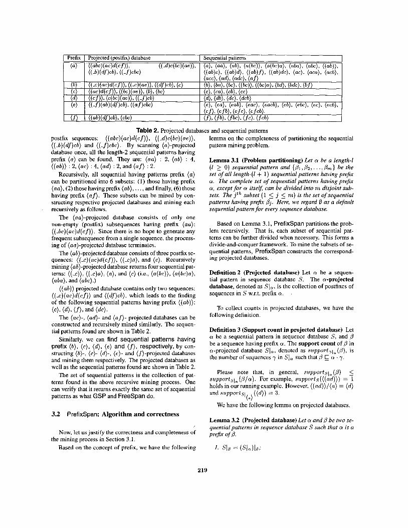
Table 2. Projected databases and sequential patterns postfix sequences: (( abc) (ac)d(cf)), (( -d)c(bc) ( a e ) ) , ((A)(#)&) and ((-f)cbc). By scanning (a)-projected database once, all the length-2 sequential patterns having prefix ( a ) can be found. They are: (a.) : 2, (ab) : 4, ( ( a b ) ) : 2, (a.) : 4, ( a d ) : 2, and (af) : 2.

Recursively, all sequential having patterns prefix ( U )

can be partitioned into 6 subsets: (1) those having prefix (aa), (2) those having prefix (ab) , . . . , and finally, (6) those having prefix (af). These subsets can be mined by constructing respective projected databases and mining each recursively as follows.

The (aa)-projected database consists of only one non-empty (postfix) subsequences having prefix (aa ) : ( ( -bc ) (ac )d (c f ) ) . Since there is no hope to generate any frequent subsequence from a single sequence, the processing of (a)-projected database terminates.

The (ab)-projected database consists of three postfix sequences: ( ( -c ) (ac)d(c f ) ) , ((-c)a), and ( c ) . Recursively mining (ab)-projected database returns four sequential patterns: ((x)), ( ( - c )a ) , ( a ) , and ( e ) (i.e., ( ~ ( b c ) ) , (a (bc )a ) , (aba), and (abc).)

( ( a b ) ) projected database contains only two sequences: ( ( - c ) ( a c ) d ( c f ) ) and ((df)cb), which leads to the finding of the following sequential patterns having prefix ( ( a b ) ) :

The (ac) - , ( ad ) - and (uf)- projected databases can be constructed and recursively mined similarly. The sequential patterns found are shown in Table 2.

Similarly, we can find sequential patterns having prefix ( b ) , ( c ) , ( d ) , (e) and (f) , respectively, by constructing (b) - , (.)- (d)-, (e)- and (f)-projected databases and mining them respectively. The projected databases as well as the sequential patterns found are shown in Table 2.

The set of sequential patterns is the collection of patterns found in the above recursive mining process. One can verify that it returns exactly the same set of sequential patterns as what GSP and FreeSpan do.

(e), (4, (f), and (dc).

3.2 Prefixspan: Algorithm and correctness

Now, let us justify the correctness and completeness of

Based on the concept of prefix, we have the following the mining process in Section 3.1.

lemma on the completeness of partitioning the sequential pattern mining problem.

Lemma 3.1 (Problem partitioning) Let a be a length4 ( 1 2 0) sequential pattern and { /31 ,& . . . pm } be the set of all length-(1 + 1) sequential patterns having prejix a. The complete set of sequential patterns having prejix a, except for a itselJ can be divided into m disjoint subsets. The j t h subset (1 < j < m) is the set of sequential patterns having prejix pi. Here, we regard 0 as a default sequential pattern for every sequence database.

Based on Lemma 3.1, Prefixspan partitions the problem recursively. That is, each subset of sequential patterns can be further divided when necessary. This forms a divide-and-conquer framework. To mine the subsets of sequential patterns, Prefixspan constructs the corresponding projected databases.

Definition2 (Projected database) Let a be a sequential pattern in sequence database S. The a-projected database, denoted as SI,, is the collection of postfixes of sequences in S w.r.t. prefix a.

To collect counts in projected databases, we have the following definition.

Definition 3 (Support count in projected database) Let a be a sequential pattern in sequence database S, and P be a sequence having prefix a. The support count of p in a-projected database SI,, denoted as s u p p o r t ~ i ~ ( P ) , is the number of sequences y in SI, such that ,6’ a . y.

Please note that, in general, supportsl_(P) 5 supportslm (p /a ) . For example, supports(((ad))) = 1 holds in our running example. However, ( ( a d ) ) / ( a ) = ( d ) and supports1 ( ( d ) ) = 3.

We have the following lemma on projected databases. (a)

Lemma 3.2 (Projected database) Let a and /3 be two sequential patterns in sequence database S such that a is a

PKBX of P.

1. SIP = ( S l a ) l p ;

219

2. for any sequence y having prejix a, supports (y) =

3. The size of a-projected database cannot exceed that supportsle (7); and

of s. Based on the above reasoning, we have the algorithm of

PrefixSpan as follows.

Algorithm 1 (Prefixspan)

Input: A sequence database S , and the minimum support

Output: The complete set of sequential patterns

Method: Call Prefixspan((), 0, S).

threshold min-sup

Subroutine PrefixSpan(a, 1, SI,) Parameters: a: a sequential pattern; 1: the length of a;

SI,: the a-projected database, if a # (); otherwise, the sequence database S.

Method:

1. Scan SI, once, find the set of frequent items b such that

(a) b can be assembled to the last element of a to

(b) ( b ) can be appended to a to form a sequential

2. For each frequent item b, append it to a to form a

3. For each a’, construct a’-projected database SI,,,

form a sequential pattern; or

pattern.

sequential pattern a’, and output a’;

and call Prefixspan (a’, 1 + 1, SI,,).

Analysis. The correctness and completeness of the algorithm can be justified based on Lemma 3.1 and Lemma 3.2, as shown in Theorem 3.1 later. Here, we analyze the efficiency of the algorithm as follows.

0 No candidate sequence needs to be generated by Prefixspan. Unlike Apriori-like algorithms, Prefixspan only grows longer sequential patterns from the shorter frequent ones. It does not generate nor test any candidate sequence nonexistent in a projected database. Comparing with GSP, which gen- erates and tests a substantial number of candidate se-

a sequence database, and thus the number of sequences in a projected database will become quite small when prefix grows; and (2) projection only takes the postfix portion with respect to a prefix. No- tice that FreeSpan also employs the idea of projected databases. However, the projection there often takes the whole string (not just postfix) and thus the shrinking factor is much less than that of Prefixspan.

0 The major cost of Prefixspanis the construction of projected databases. In the worst case, Prefixspan constructs a projected database for every sequential pattern. If there are a good number of sequential patterns, the cost is non-trivial. In Section 3.3 and Section 3.4, interesting techniques are developed, which dramatically reduces the number of projected databases.

Theorem 3.1 (Prefixspan) A sequence a is a sequential pattern ifand only if PrefixSpan says so.

3.3 Scaling up pattern growth 0y bi-level projection

As analyzed before, the major cost of Prefixspan is to construct projected databases. If the number and/or the size of projected databases can be reduced, the performance of sequential pattern mining can be improved substantially. In this section, a bi-level projection scheme is proposed to reduce the number and the size of projected databases.

Before introducing the method, let us examine the following example.

Example 4 Let us re-examine mining sequential patterns in sequence database S in Table 1. The first step is the same: Scan S to find the length-1 sequential patterns: (a ) ,

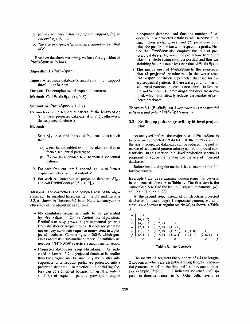
At the second step, instead of constructing projected databases for each length-1 sequential pattern, we construct a 6 x 6 lower triangular matrix M , as shown in Table 3.

( b ) , ( 4 9 ( 4 7 (e) and (f).

j quences, Prefixspan searches a much smaller space.

Projected databases keep shrinking. As indi- Table 3. The S-matrix.

cated in Lemma 3.2, a projected database is smaller than the original one because only the postfix subsequences of a frequent prefix are projected into a projected database. In practice, the shrinking factors can be significant because (1) usually, only a small set of sequential patterns grow quite long in

The matrix M registers the supports of all the length- 2 sequences which are assembled using length-I sequential patterns. A cell at the diagonal line has one counter. For example, M [ c , c] = 3 indicates sequence (cc) appears in three sequences in S. Other cells have three

220

counters respectively. For example, M [ a , c] = (4 ,2 ,1 ) means supports((ac)) = 4, supports((ca)) = 2 and supports(((ac))) = 1. Since the information in cell M[c, a] is symmetric to that in M [ a , c], a triangle matrix is sufficient. This matrix is called an S-matrix.

By scanning sequence database 5’ the second time, the S-matrix can be filled up, as shown in Table 3. All the length-2 sequential patterns can be identified from the matrix immediately.

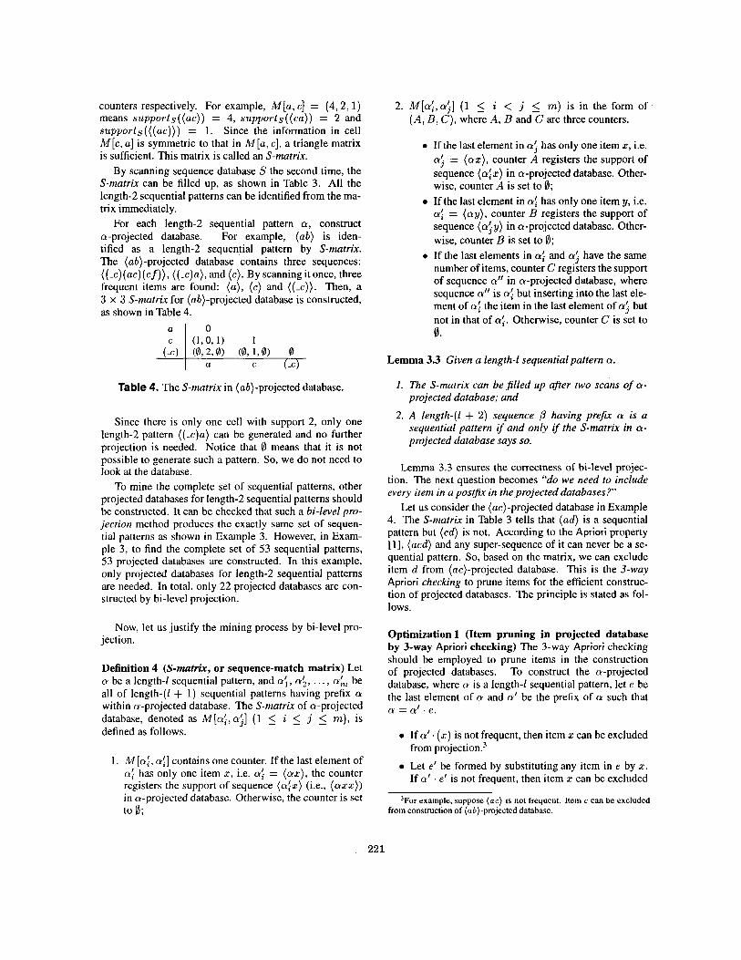
For each length-2 sequential pattern a, construct a-projected database. For example, (ab) is identified as a length-2 sequential pattern by S-matrix. The (ab)-projected database contains three sequences: ((-c)(ac)(cf)), ((-c)a), and (c). By scanningit once, three frequent items are found: (a), (c) and ((x)). Then, a 3 x 3 S-matrix for (ab)-projected database is constructed, as shown in Table 4.

(E, 1 d , l ) 1 (0,2,0) (0,1,0)

a c (-c)

Table 4. The S-matrix in (ab)-projected database.

Since there is only one cell with support 2, only one length-2 pattern ((-.)a) can be generated and no further projection is needed. Notice that 0 means that it is not possible to generate such a pattern. So, we do not need to look at the database.

To mine the complete set of sequential patterns, other projected databases for length-2 sequential patterns should be constructed. It can be checked that such a bi-level projection method produces the exactly same set of sequential patterns as shown in Example 3. However, in Exam- ple 3, to find the complete set of 53 sequential patterns, 53 projected databases are constructed. In this example, only projected databases for length-2 sequential patterns are needed. In total, only 22 projected databases are constructed by bi-level projection.

Now, let us justify the mining process by bi-level projection.

Definition 4 (S-matrix, or sequence-match matrix) Let a be a length-1 sequential pattern, and ai , a;, . . . , a; be all of length-(/ + 1) sequential patterns having prefix a within a-projected database. The S-matrix of a-projected database, denoted as M [ a : , a;] (1 5 i 5 j 5 m), is defined as follows.

1. M[a: , a:] contains one counter. If the last element of a: has only one item 2, i.e. a: = ( a z ) , the counter registers the support of sequence (ai.) (i.e., ( ~ I I ) ) in a-projected database. Otherwise, the counter is set to 0;

2. M[a:,a;] (1 5 i < j 5 m) is in the form of (A, B, C), where A, B and C are three counters.

If the last element in ai has only one item x, i.e. a: = (ax), counter A registers the support of sequence (six) in a-projected database. Other- wise, counter A is set to 0; If the last element in a: has only one item y, i.e. a: = (ay) , counter B registers the support of sequence (ai y) in a-projected database. Other- wise, counter B is set to 0; If the last elements in a: and ai have the same number of items, counter C registers the support of sequence a’’ in a-projected database, where sequence a” is a: but inserting into the last element of a: the item in the last element of a; but not in that of ai. Otherwise, counter C is set to 0.

Lemma 3.3 Given a length-1 sequential pattem a.

I . The S-matrix can be filled up after two scans of a- projected database; and

2. A length-(1 + 2 ) sequence p having prefix Q is a sequential pattern i f and only i f the S-matrix in a- projected database says so.

Lemma 3.3 ensures the correctness of bi-level projection. The next question becomes “do we need to include every item in a post@ in the projected databases?’

Let us consider the (ac)-projected database in Example 4. The S-matrix in Table 3 tells that (ad) is a sequential pattern but (cd) is not. According to the Apriori property [I], (acd) and any super-sequence of it can never be a sequential pattern. So, based on the matrix, we can exclude item d from (ac)-projected database. This is the 3-way Apriori checking to prune items for the efficient construction of projected databases. The principle is stated as follows.

Optimization 1 (Item pruning in projected database by 3-way Apriori checking) The 3-way Apriori checking should be employed to prune items in the construction of projected databases. To construct the a-projected database, where a is a length4 sequential pattern, let e be the last element of a and a’ be the prefix of a such that a = a’. e.

0 If a’. (z) is not frequent, then item z can be excluded from projection.3

Let e’ be formed by substituting any item in e by I . If a’ . e’ is not frequent, then item z can be excluded

3For example, suppose (RC) is not frequent. Item c can be excluded from construction of (ab)-projected database.

221

from the first element of postfixes if that element is a superset of e."

This optimization applies the 3-way Apriori checking to reduce projected databases further. Only fragments of sequences necessary to-grow longer patterns are projected.

3.4 Pseudo-Projection

The major cost of Prefixspan is projection, i.e., form- ing projected databases recursively. Here, we propose a pseudo-projection technique which reduces the cost of projection substantially when a projected database can be held in main memory.

By examining a set of projected databases, one can observe that postfixes of a sequence often appear repeatedly in recursive projected databases. In Example 3, sequence (a( abc) (ac)d( cf)) has postfixes (( abc) ( a c ) d ( c f ) ) and ( ( - c ) ( a c ) d ( c f ) ) as projections in (a)- and (ab)-projected databases, respectively. They are redundant pieces of sequences. If the sequence databaselprojected database can be held in main memory, such redundancy can be avoided by pseudo-projection.

The method goes as follows. When the database can be held in main memory, instead of constructing a physi- cal projection by collecting all the postfixes, one can use pointers referring to the sequences in the database as a pseudo-projection. Every projection consists of two pieces of information: pointer to the sequence in database and offset of the postfix in the sequence.

For example, suppose the sequence database S in Ta- ble l can be held in main memory. When constructing (a)-projected database, the projection of sequence s1 = (a(abc)(ac)d(cf)) consists twopieces: apointer to s1 and offser set to 2. The offset indicates that the projection starts from position 2 in the sequence, i.e., postfix (abc)(ac)d. Similarly, the projection of s1 in (ab)-projected database contains a pointer to s1 and offset set to 4, indicating the postfix starts from item c in SI.

Pseudo-projection avoids physically copying postfixes. Thus, it is efficient in terms of both running time and space. However, i t is not efficient if the pseudo-projection is used for disk-based accessing since random access disk space is very costly. Based on this observation, Prefixspan always pursues pseudo-projection once the projected databases can be held in main memory. Our experimental results show that such an integrated solution, disk-based bi-level projection for disk-based processing and pseudo-projection when data can fit into main memory, is always the clear winner in performance.

4For example, suppose ( a ( b d ) ) is not frequent. To construct (a(bc))-projected database, sequence (a (bcde )d f ) should be projected to (( -e )d f ) . The first d can be omitted. Please note that we must include the second d. Otherwise, we may fail to find pattem ( a ( b c ) d ) and those having it as a prefix.

4 Experimental Results and Performance Study

In this section, we report our experimental results on the performance of Prefixspan in comparison with GSP and Freespan. It shows that Prefixspan outperforms other previously proposed methods and is efficient and scalable for mining sequential patterns in large databases.

All the experiments are performed on a 233MHz Pen- tium PC machine with 128 megabytes main memory, running Microsoft Windows/NT. All the methods are implemented using Microsoft Visual C++ 6.0.

We compare performance of four methods as follows.

0 GSP. The GSP algorithm was implemented as described in [ l l].

0 Freespan. As reported in [6], FreeSpan with alternative level projection is more efficient than FreeSpan with level-by-level projection. In this paper, FreeSpan with alternative level projection is used.

PrefixSpan-1 is Prefixspan with level-by-level projection, as described in Section 3.2.

0 Prefixspan-1.

0 Prefixspan-2. Prefixspan-2 is Prefixspan with bi-level projection, as described in Section 3.3.

The synthetic datasets we used for our experiments were generated using standard procedure described in [2]. The same data generator has been used in most studies on sequential pattern mining, such as [ 1 1,6]. We refer readers to [ 2 ] for more details on the generation of data sets.

We test the four methods on various datasets. The results are consistent. Limited by space, we report here only the results on dataset C10T8S818. In this data set, the number of items is set to 1,000, and there are 10,000 sequences in the data set. The average number of items within elements is set to 8 (denoted as T8). The average number of elements in a sequence is set to 8 (denoted as SS). There are a good number of long sequential patterns in it at low support thresholds.

The experimental results of scalability with support threshold are shown in Figure 1. When the support threshold is high, there are only a limited number of sequential patterns, and the length of patterns is short, the four methods are close in terms of runtime. How- ever, as the support threshold decreases, the gaps become clear. Both FreeSpan and Prefixspan win GSP. PrefixSpan methods are more efficient and more scalable than FreeSpan, too. Since the gaps among FreeSpan and GSP are clear, we focus on performance of various Prefixspan techniques in the remaining of this section.

As shown in Figure 1, the performance curves of Prefixspan-1 and Prefixspan-2 are close when sup-

222

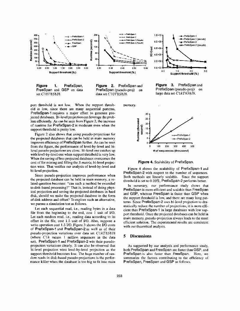
0.00 0.50 1.00 1.50 2.00 2.50 3.00

Supportthreshold (%) Support threshold (%)

c

0 0 9

+-PrefixSpafl-1 4-Prefixspan-1 (pseuQ)

8.E+09 l'E+lO1 i t Prefixspan-2 *PrefixSpan-Z (pseudo)

6.E+09

4.E+09

2.E+09

O.E+OO 0 0 1 0 20 3 0

Support threshold (%)

Figure 1. Prefixspan, Figure 2. PrefixSpan and Figure 3. PrefixSpan and FreeSpan and GSP on data PrefixSpan (pseudo-proj) on PrefixSpan (pseudo-proj) on set ClOT8S818. data set ClOT8S818. large data set ClkT8S818.

port threshold is not low. When the support threshold is low, since there are many sequential patterns, Prefixspan-1 requires a major effort to generate projected databases. Bi-level projection can leverage the problem efficiently. As can be seen from Figure 2, the increase of runtime for Prefixspan-2 is moderate even when the support threshold is pretty low.

Figure 2 also shows that using pseudo-projections for the projected databases that can be held in main memory improves efficiency of Prefixspan further. As can be seen from the figure, the performance of level-by-level and bi- level pseudo-projections are close. Bi-level one catches up with level-by-leveI one when support threshold is very low. When the saving 08 less projected databases overcomes the cost of for miningand filling the S-matrix, bi-level projection wins. That verifies our analysis of level-by-level and bi-level projection.

Since pseudo-projection improves performance when the projected database can be held in main memory, a related question becomes: "can such a method be extended to disk-based processing?' That is, instead of doing phys- ical projection and saving the projected databases in hard disk, should we make the projected database in the form of disk address and offset? To explore such an alternative, we pursue a simulation test as follows.

Let each sequential read, i.e., reading bytes in a data file from the beginning to the end, cost 1 unit of VO. Let each random read, i.e., reading data according to its offset in the file, cost 1.5 unit of VO. Also, suppose a write operation cost 1.5 VO. Figure 3 shows the VO costs of Prefixspan-1 and Prefixspan-2 as well as of their pseudo-projection variations over data set C1 kT8S818 (where Clk means 1 million sequences in the data set). Prefixspan-1 and Prefixspan-2 win their pseudo- projection variations clearly. It can also be observed that bi-level projection wins level-by-level projection as the support threshold becomes low. The huge number of random reads in disk-based pseudo-projections is the performance killer when the database is too big to fit into main

memory.

30 1

0 100 200 300 4M) 500

#of sequences (thousand)

Figure 4. Scalability of Prefixspan.

Figure 4 shows the scalability of Prefixspan-1 and Prefixspan-2 with respect to the number of sequences. Both methods are linearly scalable. Since the support threshold is set to 0.20%, Prefixspan-2 performs better.

In summary, our performance study shows that PrefixSpan is more efficient and scalable than FreeSpan and GSP, whereas FreeSpan is faster than GSP when the support threshold is low, and there are many long patterns. Since Prefixspan-2 uses bi-level projection to dramatically reduce the number of projections, it is more efficient than Prefixspan-1 in large databases with low support threshold. Once the projected databases can be held in main memory, pseudo-projection always leads to the most efficient solution. The experimental results are consistent with our theoretical analysis.

5 Discussions

As supported by our analysis and performance study, both Prefixspan and FreeSpan are faster than GSP, and PrefixSpan is also faster than FreeSpan. Here, we summarize the factors contributing to the efficiency of Prefixspan, FreeSpan and GSP as follows.

223

Both Prefixspan and FreeSpan are pattem- growth methods, their searches are more focused and thus efficient. Pattern-growth methods try to grow longer patterns from shorter ones. Accordingly, they divide the search space and focus only on the subspace potentially supporting further pattern growth at a time. Thus, their search spaces are focused and are confined by projected databases. A projected database for a sequential pattern Q

contains all and only the necessary information for mining sequential patterns that can be grown from CY. As mining proceeds to long sequential patterns, projected databases become smaller and smaller. In contrast, GSP always searches in the original database. Many irrelevant sequences have to be scanned and checked, which adds to the unnecessarily heavy cost.

0 Prefix-projected pattem growth is more elegant than frequent pattem-guided projection. Com- paring with frequent pattern-guided projection, employed in FreeSpan, prefix-projected pattern growth is more progressive. Even in the worst case, Prefixspan still guarantees that projected databases keep shrinking and only takes care postfixes. When mining in dense databases, FreeSpan cannot gain much from projections, whereas Prefixspan can cut both the length and the number of sequences in projected databases dramatically.

0 The Apriori property is integrated in bi-level projection Prefixspan. The Apriori property is the essence of the Apriori-like methods. Bi-level projection in Prefixspan applies the Apriori property in the pruning of projected databases. Based on this property, bi-level projection explores the 3-way checking to determine whether a sequential pattern can potentially lead to a longer pattern and which items should be used to assemble longer patterns. Only fruit- ful portions of the sequences are projected into the new databases. Furthermore, 3-way checking is efficient since only corresponding cells in S-matrix are checked, while no further assembling is needed.

6 Conclusions

Prefixspan mines the complete set of patterns and is efficient and runs considerably faster than both Apriori-based GSP algorithm and Freespan. Among different variations of Prefixspan, bi-level projection has better performance at disk-based processing, and pseudo-projection has the best performance when the projected sequence database can fit in main memory.

Prefixspan represents a new and promising methodology at efficient mining of sequential patterns in large databases. It is interesting to extend it towards mining sequential patterns with time constraints, time windows and/or taxonomy, and other kinds of time-related knowledge. Also, it is important to explore how to further develop such a pattern growth-based sequential pattern mining methodology for effectively mining DNA databases.

References

[ 11 R. Agrawal and R. Srikant. Fast algorithms for mining association rules. In Proc. I994 Int. Con$ Very Large Data Bases (VLDB’94), pages 487-499, Santiago, Chile, Sept. 1994.

[2] R. Agrawal and R. Srikant. Mining sequential pattems. In Proc. 1995 Int. Con$ Data Engineering (ICDE’95), pages 3-14, Taipei, Taiwan, Mar. 1995.

[3] C. Bettini, X. S. Wang, and S. Jajodia. Mining temporal relationships with multiple granularities in time sequences. Data Engineering Bulletin, 21:32-38, 1998.

[4] M. Garofalakis, R. Rastogi, and K. Shim. Spirit: Sequen- tial pattem mining with regular expression constraints. In Proc. I999 Int. Con$ Very Large Data Bases (VLDB’99), pages 223-234, Edinburgh, UK, Sept. 1999.

[5] J. Han, G. Dong, and Y. Yin. Efficient mining of partial periodic pattems in time series database. In Proc. 1999 Int. Conj Data Engineering (ICDE‘99), pages 106-1 15, Sydney, Australia, Apr. 1999.

[6] J . Han, J. Pei, B. Mortazavi-Asl, Q. Chen, U. Dayal, and M.-C. Hsu. Freespan: Frequent pattem-projected sequential pattem mining. In Proc. 2000 Int. Con$ Knowledge Discovery and Data Mining (KDD’OO), pages 355-359, Boston, MA, Aug. 2000.

[7] J. Han, J. Pei, and Y. Yin. Mining frequent pattems without candidate generation. In Proc. 2000 ACM-SIGMOD Int. Con$ Management of Data (SIGMOD’OO), pages 1- 12, Dallas, TX, May 2000.

[8] H. Lu, J. Han, and L. Feng. Stock movement and n- dimensional inter-transaction association rules. In Proc. I998 SIGMOD Workshop Research Issues on Data Mining and Knowledge Discove-ry (DMKD’98), pages 12:l-12:f Seattle, WA, June 1998.

[9] H. ~ ~ ~ ~ i l ~ , H. ~ ~ i ~ ~ ~ ~ ~ , and A. 1. Verkamo. Discovery of frequent episodes in event sequences. Data Mining and Knowledge Discovery, 1 :259-289,1997.

[IO1 B. Ozden. s. Ramaswamy, and A. Silberschatz. cyclic association rules. In Proc. I998 Int. Con$ Data Engineering (ICDE’98), pages 412-421, Orlando, FL, Feb. 1998.

[l 11 R. Srikant and R. Agrawal. Mining sequential pattems: Generalizations and performance improvements. In Proc. 5th Int. Con$ Extending Database Technology (EDBT’96), pages 3-17, Avignon, France, Mar. 1996.

In this paper, we have developed a novel, scalable, and efficient sequential mining method, called Prefixspan. Its general idea is to examine only the prefix subsequences and project only their corresponding postfix subsequences into projected databases. In each projected database, sequential patterns are grown by exploring only local frequent patterns. To further improve mining efficiency, two kinds of database projections are explored: level-by- level projection and bi-level projection, and an optimization technique which explores pseudo-projection is developed. Our systematic performance study shows that

224

prefixspan,: mining sequential patterns efficiently by

Documents