SLIDE 1Predictive Indicators

MESA SoftwareJohn Ehlers

e-mail: ehlers@mesasoftware.com

SLIDE 2AGENDA

Exponential Moving Averages• Why lag is important• How to compute the EMA constant to produce a given lag

Higher order filters• Let your computer do a superior job of smoothing

Essence of Predictive Filters Linear Kalman Filters Nonlinear Kalman Filters Theoretically Optimum Predictive Filters Zero Lag smoothing

SLIDE 3

Fundamental Conceptof Predictive Filters

In the trend mode price difference is directly related to time lag

Procedure to generate a predictive line:• Take an EMA of price (better, a 3 Pole filter)• Take the difference ( delta) between the price and its EMA• Form the predictor by adding delta to the price

– equivalent to adding 2*delta to EMA

SLIDE 4

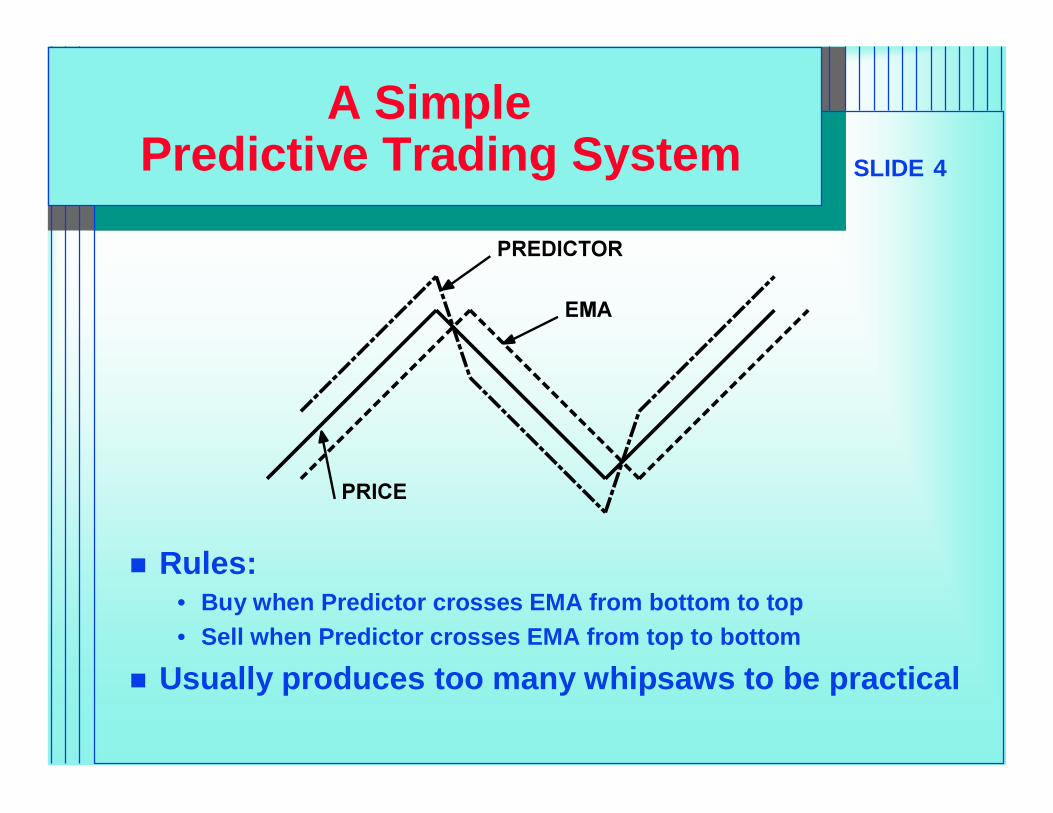
A SimplePredictive Trading System

Rules:• Buy when Predictor crosses EMA from bottom to top• Sell when Predictor crosses EMA from top to bottom

Usually produces too many whipsaws to be practical

SLIDE 5Secrets of Predictive Filters

All averages lag (and smooth) All differences lead (and are more noisy) The objective of filters is to eliminate the

unwanted frequency components The range of trading frequencies makes a

single filter approach impractical A better approach divides the market into two

modes• Cycle Mode• Trend Mode

– A Trend can be a piece of a longer cycle

SLIDE 6

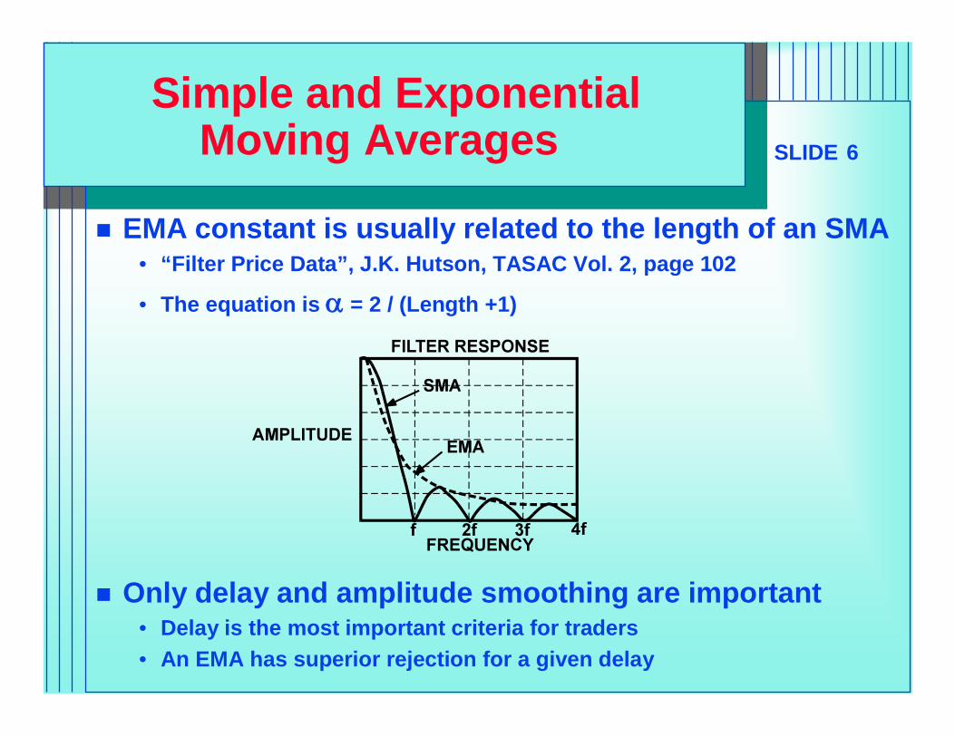
Simple and ExponentialMoving Averages

EMA constant is usually related to the length of an SMA• “Filter Price Data”, J.K. Hutson, TASAC Vol. 2, page 102

• The equation is = 2 / (Length +1)

Only delay and amplitude smoothing are important• Delay is the most important criteria for traders• An EMA has superior rejection for a given delay

SLIDE 7

Relating Lagto the EMA Constant

An EMA is calculated as:g(z) = *f(z) + (1 - )*g(z - 1)

where g() is the outputf() is the inputz is the incrementing variable

Assume the following for a trend mode• f() increments by 1 for each step of z

– has a value of “i” on the “i th” day• k is the output lagi - k = *i + (1 - )*(i - k - 1)

= *i + (i - k) - 1 - *i + *(k + 1)0 = *(k + 1) - 1

Then k = 1/ -1 OR = 1/(k + 1)

SLIDE 8

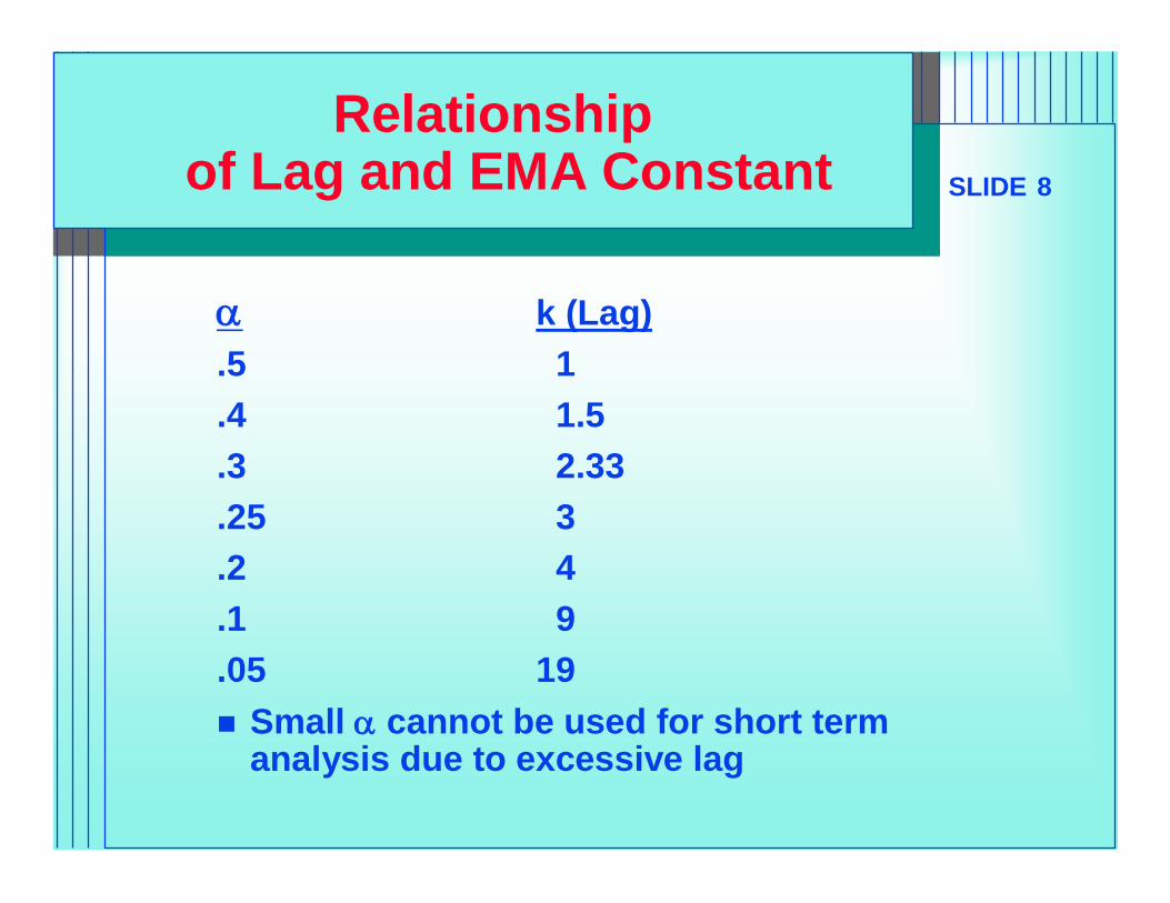
Relationshipof Lag and EMA Constant

k (Lag).5 1.4 1.5.3 2.33.25 3.2 4.1 9.05 19 Small cannot be used for short term

analysis due to excessive lag

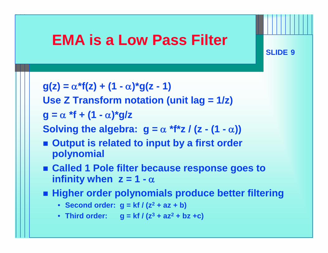
SLIDE 9EMA is a Low Pass Filter

g(z) = *f(z) + (1 - )*g(z - 1)Use Z Transform notation (unit lag = 1/z)g = *f + (1 - )*g/zSolving the algebra: g = *f*z / (z - (1 - )) Output is related to input by a first order

polynomial Called 1 Pole filter because response goes to

infinity when z = 1 - Higher order polynomials produce better filtering

• Second order: g = kf / (z2 + az + b)• Third order: g = kf / (z3 + az2 + bz +c)

SLIDE 10

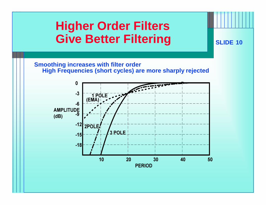
Higher Order FiltersGive Better Filtering

Smoothing increases with filter orderHigh Frequencies (short cycles) are more sharply rejected

SLIDE 11

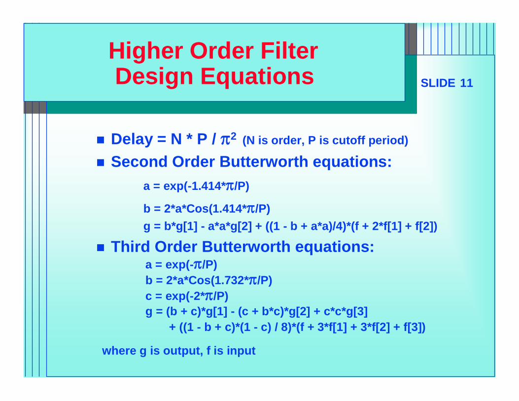
Higher Order FilterDesign Equations

Delay = N * P / 2 (N is order, P is cutoff period)

Second Order Butterworth equations:a = exp(-1.414*/P)

b = 2*a*Cos(1.414*/P)g = b*g[1] - a*a*g[2] + ((1 - b + a*a)/4)*(f + 2*f[1] + f[2])

Third Order Butterworth equations: a = exp(-/P)b = 2*a*Cos(1.732*/P)c = exp(-2*/P)g = (b + c)*g[1] - (c + b*c)*g[2] + c*c*g[3]

+ ((1 - b + c)*(1 - c) / 8)*(f + 3*f[1] + 3*f[2] + f[3])

where g is output, f is input

SLIDE 12

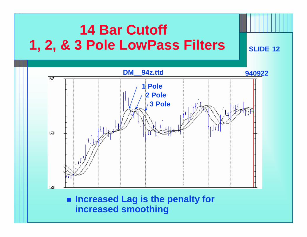
14 Bar Cutoff1, 2, & 3 Pole LowPass Filters

Increased Lag is the penalty for increased smoothing

1 Pole2 Pole

3 Pole

DM__94z.ttd 940922

SLIDE 13

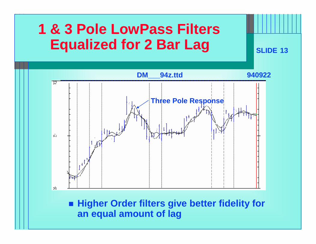
Higher Order filters give better fidelity for an equal amount of lag

1 & 3 Pole LowPass FiltersEqualized for 2 Bar Lag

Three Pole Response

DM___94z.ttd 940922

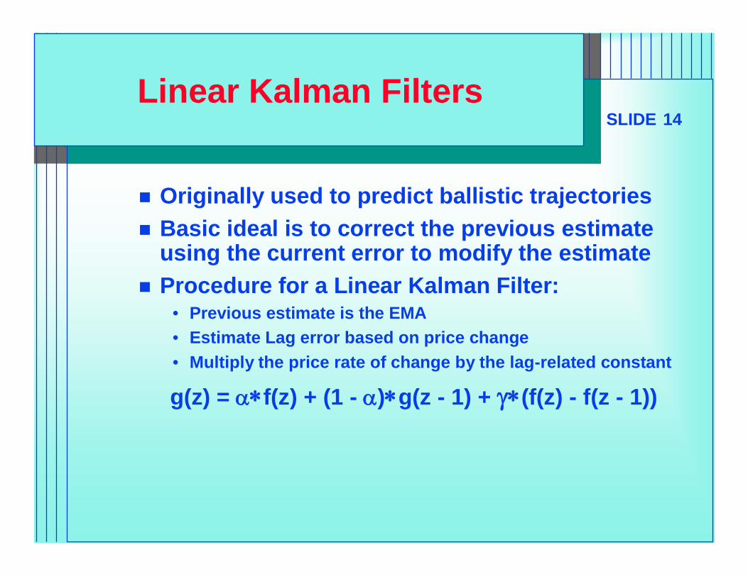
SLIDE 14Linear Kalman Filters

Originally used to predict ballistic trajectories Basic ideal is to correct the previous estimate

using the current error to modify the estimate Procedure for a Linear Kalman Filter:

• Previous estimate is the EMA• Estimate Lag error based on price change• Multiply the price rate of change by the lag-related constant

g(z) = f(z) + (1 - )g(z - 1) + (f(z) - f(z - 1))

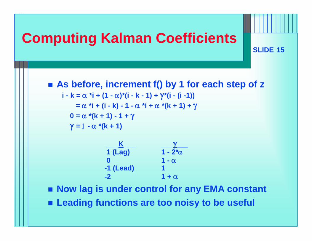
SLIDE 15Computing Kalman Coefficients

As before, increment f() by 1 for each step of zi - k = *i + (1 - )*(i - k - 1) + *(i - (i -1))

= *i + (i - k) - 1 - *i + *(k + 1) + 0 = *(k + 1) - 1 + = - *(k + 1)

___K___ _____1 (Lag) 1 - 2*0 1 -

-1 (Lead) 1-2 1 +

Now lag is under control for any EMA constant Leading functions are too noisy to be useful

SLIDE 16

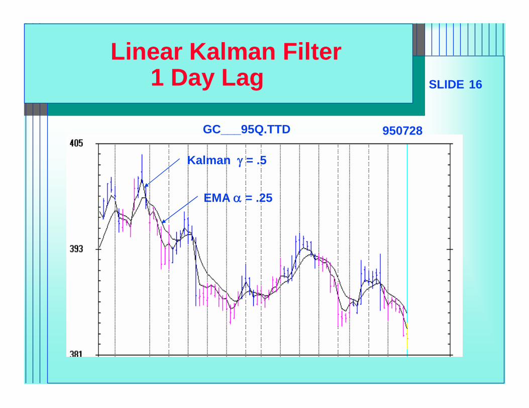
Linear Kalman Filter1 Day Lag

GC___95Q.TTD 950728

EMA = .25

Kalman = .5

SLIDE 17Nonlinear Kalman Filter

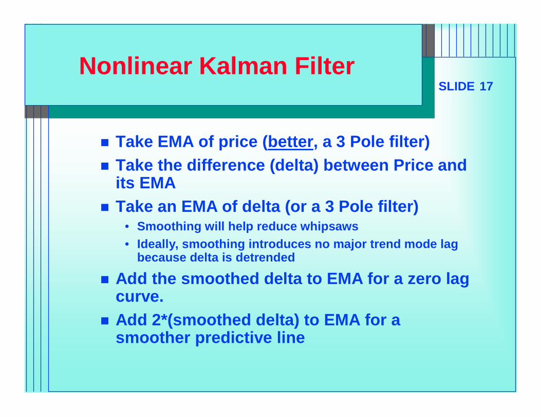
Take EMA of price (better, a 3 Pole filter) Take the difference (delta) between Price and

its EMA Take an EMA of delta (or a 3 Pole filter)

• Smoothing will help reduce whipsaws• Ideally, smoothing introduces no major trend mode lag

because delta is detrended

Add the smoothed delta to EMA for a zero lag curve.

Add 2*(smoothed delta) to EMA for a smoother predictive line

SLIDE 18

Zero LagNonlinear Kalman Filter Example

GC___95Q.TTD 950728

EMA = .25

Nonlinear Kalman Response

SLIDE 19

Theoretically OptimumPredictive Filters

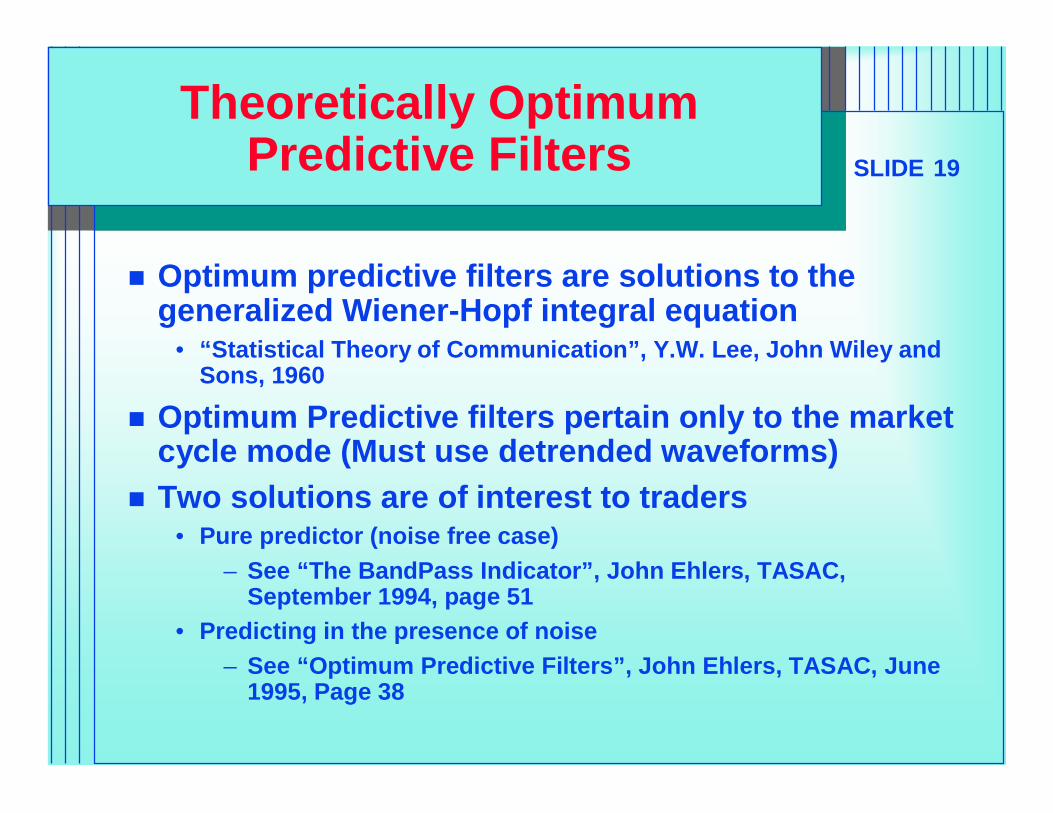
Optimum predictive filters are solutions to the generalized Wiener-Hopf integral equation

• “Statistical Theory of Communication”, Y.W. Lee, John Wiley and Sons, 1960

Optimum Predictive filters pertain only to the market cycle mode (Must use detrended waveforms)

Two solutions are of interest to traders• Pure predictor (noise free case)

– See “The BandPass Indicator”, John Ehlers, TASAC, September 1994, page 51

• Predicting in the presence of noise– See “Optimum Predictive Filters”, John Ehlers, TASAC, June

1995, Page 38

SLIDE 20Pure Predictor

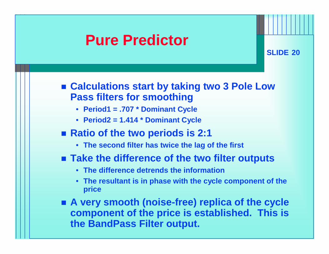
Calculations start by taking two 3 Pole Low Pass filters for smoothing

• Period1 = .707 * Dominant Cycle• Period2 = 1.414 * Dominant Cycle

Ratio of the two periods is 2:1• The second filter has twice the lag of the first

Take the difference of the two filter outputs• The difference detrends the information• The resultant is in phase with the cycle component of the

price

A very smooth (noise-free) replica of the cycle component of the price is established. This is the BandPass Filter output.

SLIDE 21

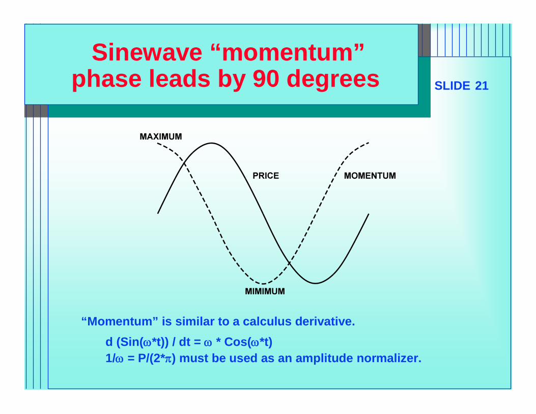
Sinewave “momentum”phase leads by 90 degrees

“Momentum” is similar to a calculus derivative.d (Sin(*t)) / dt = * Cos(*t)1/ = P/(2*) must be used as an amplitude normalizer.

SLIDE 22

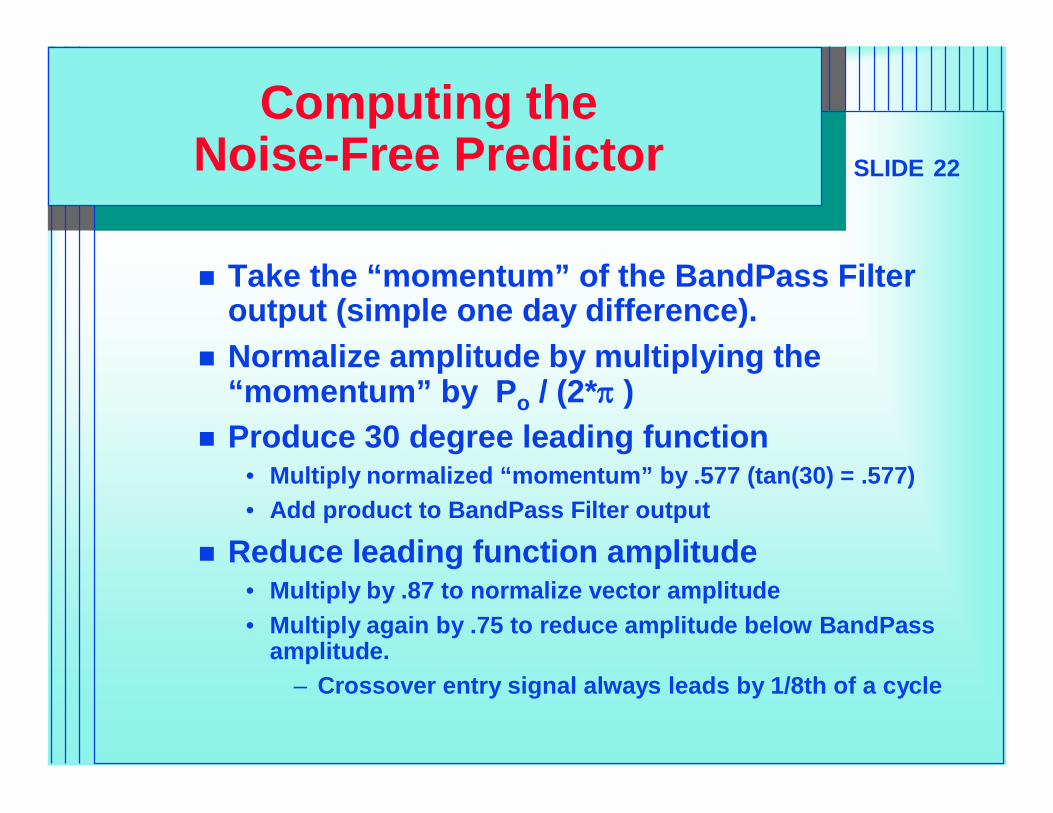
Computing the Noise-Free Predictor

Take the “momentum” of the BandPass Filter output (simple one day difference).

Normalize amplitude by multiplying the “momentum” by Po / (2* )

Produce 30 degree leading function • Multiply normalized “momentum” by .577 (tan(30) = .577)• Add product to BandPass Filter output

Reduce leading function amplitude• Multiply by .87 to normalize vector amplitude• Multiply again by .75 to reduce amplitude below BandPass

amplitude.– Crossover entry signal always leads by 1/8th of a cycle

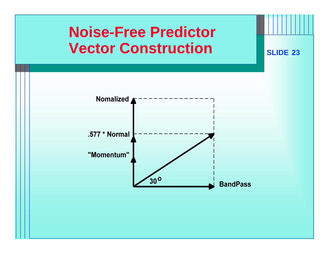
SLIDE 23

Noise-Free PredictorVector Construction

SLIDE 24

The Complete BandPass Indicator

The BandPass Indicator is automatically tuned in:• MESA for Windows• 3D for Windows

SLIDE 25

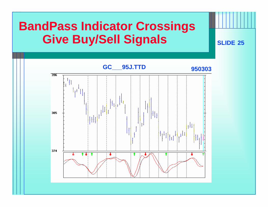
BandPass Indicator CrossingsGive Buy/Sell Signals

GC___95J.TTD 950303

SLIDE 26

Optimum Predictive Filterin the Presence of Noise

Start with RSI or Stochastic Indicator• Provides detrended waveform• Adjust length until the waveform resembles a sinewave

Technique is useful only when the waveform has a Poisson probability distribution

• The midpoint crossings must be relatively regular

Take an EMA of the RSI� = .25 is nominally correct (gives a 3 day lag)

Subtract the EMA from the RSI to produce the predictor

• Remember the fundamental premise in constructing predictive filters?

SLIDE 27

RSI and Optimum Predictive Filter

GC___95J.TTD 950303

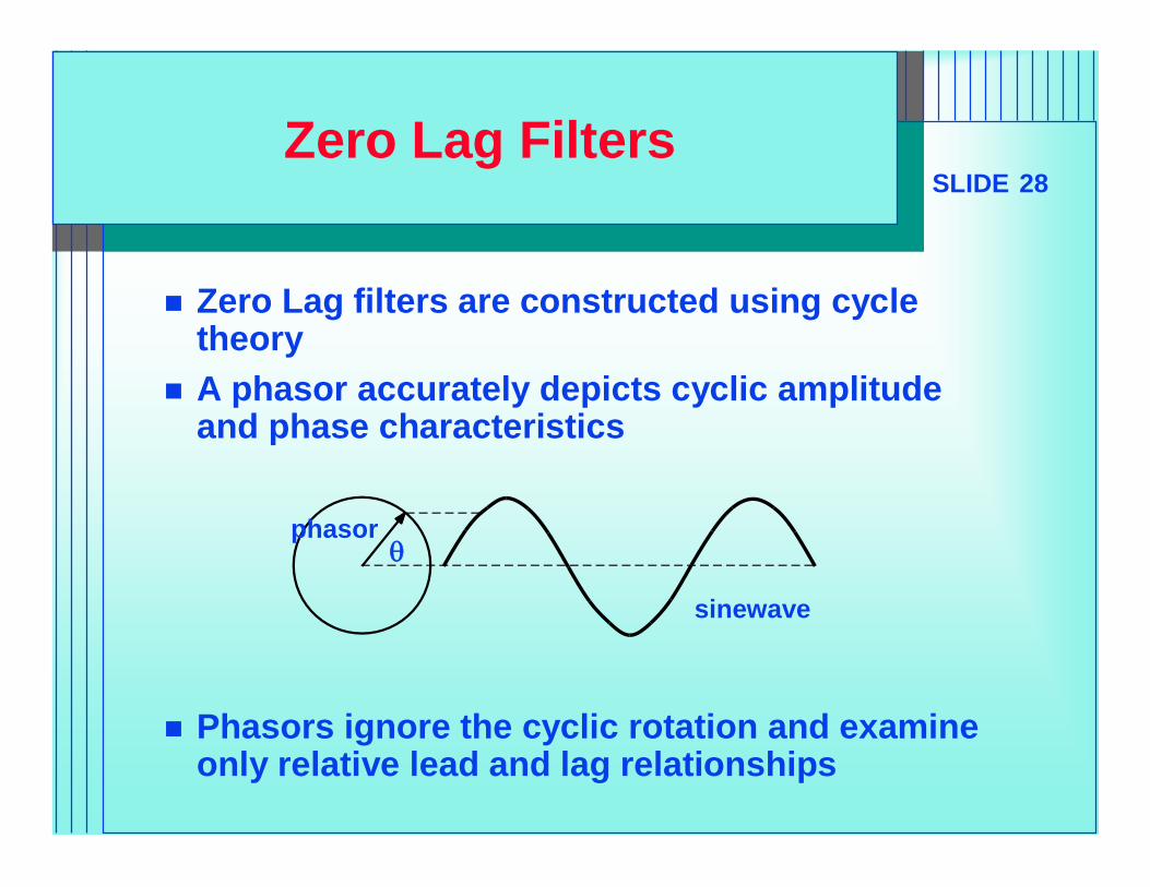
SLIDE 28Zero Lag Filters

Zero Lag filters are constructed using cycle theory

A phasor accurately depicts cyclic amplitude and phase characteristics

Phasors ignore the cyclic rotation and examine only relative lead and lag relationships

sinewave

phasor

SLIDE 29Zero Lag Filter Construction

Phasor A has a lag of DominantCycle/16

Phasor B has twice the lag of Phasor A

Subtract B from A by reversing B and adding

Resultant is detrendedleading angle Phasor C

Vector add C to A Resultant is zero lag,

non-detrended Phasor D

AB

A

-BC

C

AD

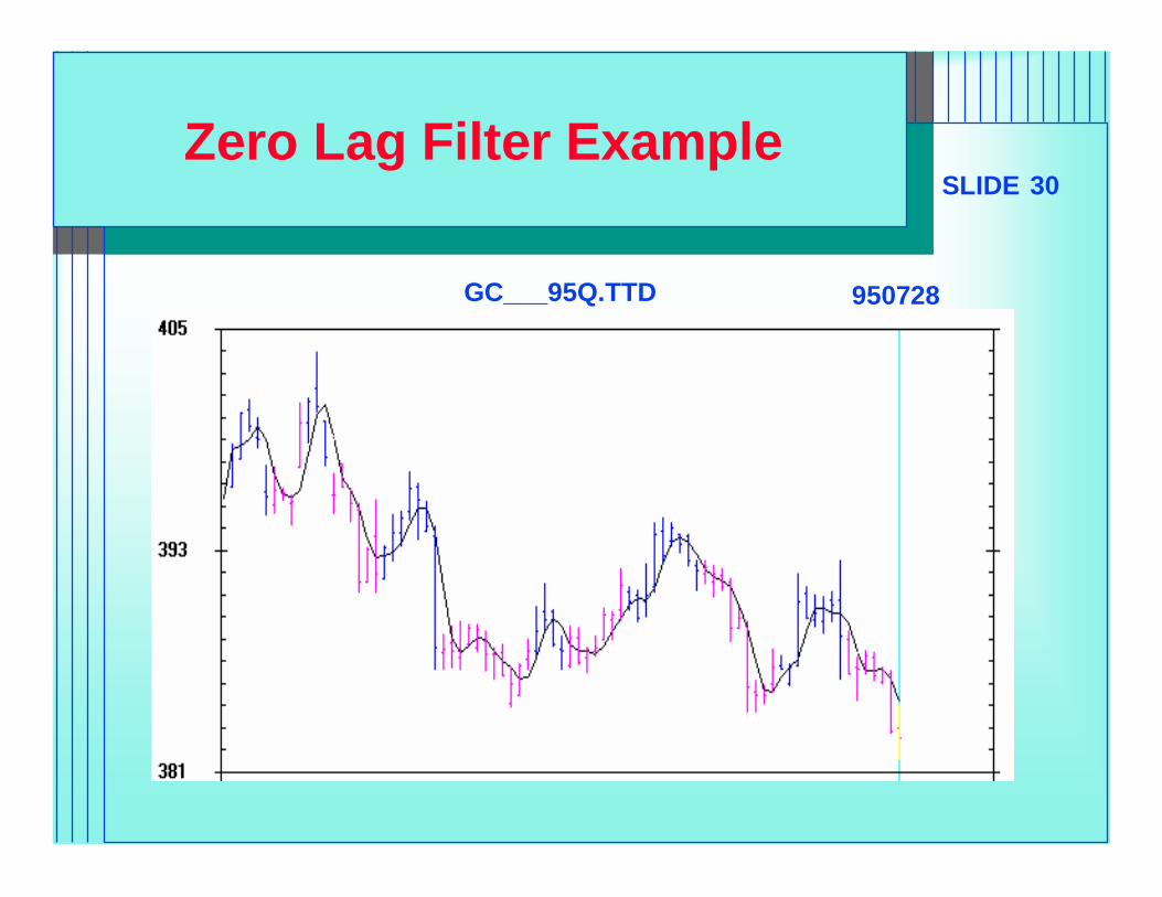
SLIDE 30Zero Lag Filter Example

GC___95Q.TTD 950728

SLIDE 31A Zero Lag Filter Application

Take a 3 Pole zero lag filter of price highs Take a 3 Pole zero lag filter of price lows Calculate statistics of the high and low

variations• Add 2 Standard Deviations to the Highs Zero Lag Filter• Subtract 2 Standard Deviations to the Lows Zero Lag Filter

Resultant channels can be used as stop values for a stop-and-reverse system

Remove the +/- Std Deviations near cycle turns SUMMIT for Windows uses this procedure

SLIDE 32SUMMARY

What you have learned:• How to relate filter lag to EMA constant• How to compute Higher Order Butterworth Filters• How to control lag using a Linear Kalman Filter• How to compute a Nonlinear Kalman Filter

– Possible start for a crossover system• How to compute Optimum Predictive Filters for the cycle

mode– Pure Predictor (Noise-Free, using higher order filters)– With RSI or Stochastics

• How to compute a zero lag filter